Entropy-Based Sim(3) Calibration of 2D Lidars to Egomotion Sensors

Abstract

This paper explores the use of an entropy-based technique for point cloud reconstruction with the goal of calibrating a lidar to a sensor capable of providing egomotion information. We extend recent work in this area to the problem of recovering the Sim(3) transformation between a 2D lidar and a rigidly attached monocular camera, where the scale of the camera trajectory is not known a priori. We demonstrate the robustness of our approach on realistic simulations in multiple environments, as well as on data collected from a hand-held sensor rig. Given a non-degenerate trajectory and a sufficient number of lidar measurements, our calibration procedure achieves millimetre-scale and sub-degree accuracy. Moreover, our method relaxes the need for specific scene geometry, fiducial markers, or overlapping sensor fields of view, which had previously limited similar techniques.

I INTRODUCTION

Multisensor payloads have become the norm in many mobile robotic systems. In particular, lidars are frequently used on multisensor platforms that must estimate distances accurately. While visual sensors such as stereo cameras can recover this information using multiple view geometry, they do not have the accuracy of typical lidars for depth estimation [1]. Inexpensive RGB-D cameras are also commonly used for building dense, coloured 3D maps, but they have limited range and are generally too sensitive to lighting conditions to be used outdoors. In fact, modern 3D lidars are commonly employed to generate ground truth depth maps against which to evaluate the performance of visual estimation techniques [2]. The range and lighting-invariance of a lidar makes it suitable for both indoor and outdoor operation; lidars have proven to be an unparalleled sensor choice for unmanned ground vehicles such as self-driving cars[3, 4].

(a) Point cloud before calibration.

(b) Point cloud after calibration using our method.

Figure 1: Visualization of a point cloud collected in the environment pictured in Figure 6, using initial values and mean values from Table III. Note the smooth wall segments on the right side of Figure 1(b).

Robotic platforms will often include both cameras and lidars as complementary sensors. Cameras provide dense visual information, but in the form of 2D images which complicates the recovery of 3D information. Moreover, in the case of monocular motion estimation, a scale ambiguity exists: metric scale cannot be recovered from monocular images alone. In contrast, lidars provide precise range information, ideal for creating depth maps and naturally complementing camera data in scene reconstruction [5].

In general, successfully combining information from multiple sensors requires knowledge of the coordinate transformations between them—an inaccurate transform leads to systematic error in the fused sensor data. Manually measuring the translational and rotational offset between sensors is inaccurate and may be impractical since the origins of the sensor coordinate systems are often embedded within the sensors themselves. Instead, we would like to use data-driven techniques to estimate the sensor-to-sensor transformations. Conventional approaches to this problem often require a specific calibration procedure with a target (e.g., a checkerboard in the case of cameras), although techniques have been developed recently for automatic calibration “in the wild”. Despite these advances, current methods show a lack of generality in that they are often developed for specific sensor suites, require specialized scene structure, or place restrictions on the sensors’ fields of view (FOVs). These limitations are especially problematic for long-term robotic deployments, during which the extrinsic calibration parameters may slowly drift or suddenly change; a calibration procedure applicable to an unknown environment and sensor configuration would then be necessary.

In this work, we seek to address these limitations by developing a generalized technique for the extrinsic calibration of a 2D lidar to a sensor capable of providing egomotion information. Our method builds directly upon previous work [6, 7] by representing the lidar point cloud as a Gaussian Mixture Model (GMM) and minimizing its Rényi Quadratic Entropy (RQE) in order to recover the coordinate transformation between the two sensors. In contrast to [6, 7], which are concerned with estimating SE(3) rigid body transformations between sensor pairs, we estimate Sim(3) similarity transformations. This allows us to use a monocular camera as the egomotion sensor, despite the scale ambiguity in its trajectory reconstruction. The scale factor is estimated as part of the calibration process.

The remainder of the paper is organized as follows: Section II situates our paper with respect to existing literature. Sections III and IV lay out the mathematical underpinnings of our approach as well as practical considerations in its implementation. In Section V, we show through simulations that we can recover the Sim(3) transformation between a lidar and a noisy egomotion sensor. Experiments presented in Section VI demonstrate that our technique can also recover the absolute scale of a trajectory estimated from a monocular image stream. We show that our technique performs reliably even in environments with complex structures. Finally, we conclude by motivating the development of a spatiotemporal calibration technique based on entropy minimization.

II RELATED WORK

Extrinsic sensor calibration is an active area of research and a variety of approaches have been developed. The classic approach for extrinsic calibration involves a laboratory procedure making use of a known calibration object. For cameras and 2D lidars, a common choice is to identify lines on a planar calibration target [8, 9, 10]. More complex patterned planes have also been used in some work [11, 12].

As a step towards removing the need for specific calibration objects, several methods instead attempt to identify appropriate calibration geometry (‘features’) in the environment. For example, surface normals can be extracted from lidar data and processed for comparison with camera images [13, 14]. Picking out linear features, typically lines formed at the intersection of planar surfaces, is a practical option in indoor environments [15, 16]. Note, however, that all the methods mentioned thus far require the camera and lidar to simultaneously observe the same features, which requires an overlapping FOV between the two sensors.

Some recent techniques relax the overlapping FOV requirement, by allowing each sensor to observe the same features at different times [17, 18, 19]. These approaches also require accurate temporal alignment of the sensor data. While spatiotemporal calibration techniques are few, the case of non-overlapping lidar and stereo cameras has been addressed by identifying and matching planar surfaces[20]. The method of [20] represents a significant step towards generalized spatiotemporal calibration, but requires specific features and metrically accurate trajectory estimates.

In contrast to previous work, our technique (an extension of [21] and [7]) requires neither overlapping FOVs, nor observations of specific features in the environment. We assume only a non-degenerate sensor trajectory[22] and a scene with a certain level of structure, as discussed in Section VII. Metric accuracy is not necessary, as we explicitly optimize for scale.

III THEORY

III-A Problem Formulation

For our particular application, we assume that the camera’s intrinsic parameters have been calibrated and that a monocular motion estimation system (e.g. ORB-SLAM [23]) provides a reasonable sensor trajectory, accurate up to a scale factor. We stress that this method is not restricted to monocular cameras; any sensor capable of providing egomotion estimates (i.e., the base sensor) could be used in place of the camera.

The base sensor provides a set of $K$ 6DOF poses, $\mathbf{Y}$:

$$\mathbf{Y}=\{\mathbf{y}_{1},\mathbf{y}_{2},...,\mathbf{y}_{K}\},~{}~{}\mathbf{y}_{k}=\left[x_{k}~{}y_{k}~{}z_{k}~{}\phi_{k}~{}\theta_{k}~{}\psi_{k}\right]^{T},$$ (1)

where $\phi$, $\theta$ and $\psi$ are roll, pitch and yaw Euler angles, respectively. Each pose $\mathbf{y}_{k}$ has an associated timestamp $t_{k}$ and pose covariance matrix $\mathbf{Q}_{k}$. The lidar provides a set of $K\times N$, 2D observations, $\mathbf{Z}$, where:

$$\mathbf{Z}=\{\mathbf{z}_{1},\mathbf{z}_{2},...,\mathbf{z}_{K}\},~{}~{}\mathbf{z}_{k}=\{\mathbf{z}^{(1)}_{k},\mathbf{z}^{(2)}_{k},...,\mathbf{z}^{(N)}_{k}\},$$ (2)

$$\mathbf{z}^{(n)}_{k}=\left[x^{(n)}_{k}~{}y^{(n)}_{k}\right]^{T},$$ (3)

and each point $\mathbf{z}^{(n)}_{k}$ has associated timestamp $t_{k}$. We assume that the camera and lidar measurements are temporally aligned and explore the consequences of this assumption in Section V-E. For convenience, we adopt a homogeneous representation and express each point in lidar frame $\underrightarrow{\mathcal{F}}_{L_{k}}$ as

$$\mathbf{p}^{(n)}_{L_{k}}=\left[x^{(n)}_{k}~{}y^{(n)}_{k}~{}0~{}1\right]^{T}.$$ (4)

Likewise, we express each camera pose as a homogeneous transformation from camera frame $\underrightarrow{\mathcal{F}}_{C_{k}}$ to a fixed global frame $\underrightarrow{\mathcal{F}}_{G}$, where matrix $\mathbf{T}_{G,C_{k}}$ is the homogeneous representation of pose $\mathbf{y}_{k}$.

Our goal is to estimate the set of (constant) transform parameters from the lidar frame $\underrightarrow{\mathcal{F}}_{L}$ to the camera frame $\underrightarrow{\mathcal{F}}_{C}$

$$\boldsymbol{\Xi}=\left[x_{L}~{}~{}y_{L}~{}~{}z_{L}~{}~{}\phi_{L}~{}~{}\theta_{L}~{}~{}\psi_{L}~{}~{}s\right]^{T},$$ (5)

which we use to form the rigid body transformation matrix $\mathbf{T}_{{C},{L}}$ from $\underrightarrow{\mathcal{F}}_{L}$ to $\underrightarrow{\mathcal{F}}_{C}$. The scale factor, $s$, is applied in the transformation from the camera frame to global frame. This defines our inverse sensor model, with which we can estimate the position of a lidar point in the global frame:

$$\hat{\mathbf{p}}^{(n)}_{G,k}=h^{-1}(\mathbf{p}^{(n)}_{L_{k}}\mid\mathbf{y}_{k},\boldsymbol{\Xi})=\mathbf{T}_{G,C_{k}}\mathbf{T}_{{C_{k}},{L_{k}}}\mathbf{p}^{(n)}_{L_{k}}.$$ (6)

Omitting the homogeneous component so that $\hat{\mathbf{x}}^{(n)}_{G,k}\leftarrow\hat{\mathbf{p}}^{(n)}_{G,k}$, we use the Jacobian of this model and the camera pose covariances to obtain a covariance estimate of points in the world frame:

$$\boldsymbol{\Sigma}^{(n)}_{k}=\mathbf{J}^{(n)}_{k}\mathbf{Q}_{k}{\mathbf{J}^{(n)}_{k}}^{T},~{}~{}\mathbf{J}^{(n)}_{k}=\dfrac{\partial h^{-1}(\mathbf{x}^{(n)}_{L_{k}}|\mathbf{y}_{k},\boldsymbol{\Xi})}{\partial\mathbf{y}_{k}}.$$ (7)

Finally, we obtain a set of 3D points $\hat{\mathbf{x}}^{(n)}_{G,k}\in\hat{\mathbf{X}}$ expressed in the global frame, each with an associated 3 $\times$ 3 covariance matrix $\boldsymbol{\Sigma}^{(n)}_{k}$ and timestamp $t^{(n)}_{k}$.

III-B Point Cloud Rényi Quadratic Entropy

As in [7], we minimize the Rényi Quadratic Entropy (RQE) [24] in order to maximize the compactness or ‘crispness’ of the estimated point cloud $\hat{\mathbf{X}}$. The intuition behind maximizing point cloud compactness follows from the assumption that the surfaces in the environment are structured 2D manifolds as opposed to diffuse, random elements. This assumption holds particularly well in many urban and natural scenes.

The RQE of the continuous random variable $X$ with probability distribution $p(\mathbf{x})$ is defined as:

$$H[X]=-\log\int p(\mathbf{x})^{2}d\mathbf{x}.$$ (8)

We represent our point cloud $\hat{\mathbf{X}}$ as a Gaussian mixture model (GMM), where $p(\mathbf{x})$ is the probability of a lidar measurement being sampled at position $\mathbf{x}$ given centroids $\{\hat{\mathbf{x}}_{1},...,\hat{\mathbf{x}}_{M}\}\in\hat{\mathbf{X}}$:

$$p(\mathbf{x})=\frac{1}{M}\sum_{i=1}^{M}\mathcal{N}(\mathbf{x}-\hat{\mathbf{x}}_{i},\boldsymbol{\Sigma}_{i}+\sigma^{2}\mathbf{I}),$$ (9)

where the covariance includes pose uncertainty $\mathbf{\Sigma}_{i}$ calculated using Equation 7, and measurement uncertainty in the isotropic kernel $\sigma^{2}\mathbf{I}$. Note that $M$ may be less than $K\times N$ due to missing lidar measurements (e.g., out of range readings). An analytic representation of the RQE of the GMM can be derived as

$$H[\hat{\mathbf{X}}]= -\log\int\biggl{(}\frac{1}{M}\sum_{i=1}^{M}\mathcal{N}(\mathbf{x}-\hat{\mathbf{x}}_{i},\boldsymbol{\Sigma}_{i}+\sigma^{2}\mathbf{I})\biggr{)}^{2}d\mathbf{x}$$ (10)

$$= -\log\biggl{(}\frac{1}{M^{2}}\sum_{i=1}^{M}\sum_{j=1}^{M}\int\mathcal{N}(\mathbf{x}-\hat{\mathbf{x}}_{i},\boldsymbol{\Sigma}_{i}+\sigma^{2}\mathbf{I})$$ (11)

$$~{}~{}~{}~{}~{}~{}~{}~{}~{}~{}~{}~{}~{}~{}~{}~{}~{}~{}~{}~{}~{}~{}~{}~{}\mathcal{N}(\mathbf{x}-\hat{\mathbf{x}}_{j},\boldsymbol{\Sigma}_{j}+\sigma^{2}\mathbf{I})d\mathbf{x}\biggr{)}$$

$$= -\log\biggl{(}\frac{1}{M^{2}}\sum_{i=1}^{M}\sum_{j=1}^{M}\mathcal{N}(\hat{\mathbf{x}}_{i}-\hat{\mathbf{x}}_{j},\boldsymbol{\Sigma}_{i}+\boldsymbol{\Sigma}_{j}+2\sigma^{2}\mathbf{I})\biggr{)}.$$ (12)

Therefore, to calculate the entropy of a GMM, we must compute all pairwise entropy contributions.

IV Algorithm

Using Equation 12, we wish to solve for the optimal set of calibration parameters $\boldsymbol{\Xi}^{*}$ which minimizes the total point cloud entropy. For optimization, the cost function can be simplified greatly. First, we can trivially remove the monotonic logarithm function and constant $1/M^{2}$ factor. Next, we note that for each pair of points $\left(\hat{\mathbf{x}}_{i},\hat{\mathbf{x}}_{j}\right)\in\hat{\mathbf{X}}$, we are calculating their pairwise entropy contribution twice, as seen in the indices of the sums in Equation 12. We can therefore solve the equivalent problem[7]:

$$\boldsymbol{\Xi}^{*}=\operatorname*{argmin}_{\boldsymbol{\Xi}}~{}-\sum_{i=1}^{M}\sum_{j=i}^{M}\mathcal{N}(\hat{\mathbf{x}}_{i}-\hat{\mathbf{x}}_{j},\boldsymbol{\Sigma}_{i}+\boldsymbol{\Sigma}_{j}+2\sigma^{2}\mathbf{I}),$$ (13)

noting that the coordinates of each point $\hat{\mathbf{x}}_{i},\hat{\mathbf{x}}_{j}$ are functions of the calibrations parameters and the camera poses.

Moreover, a large majority of point pairs contribute negligible entropy. We can avoid unnecessary computation by setting a conservative upper bound on the pairwise distance:

$$\mathcal{N}(\hat{\mathbf{x}}_{i}-\hat{\mathbf{x}}_{j},\boldsymbol{\Sigma}_{i}+\boldsymbol{\Sigma}_{j}+2\sigma^{2}\mathbf{I})\approx 0~{}~{}\mathrm{if}$$

$$||\hat{\mathbf{x}}_{i}-\hat{\mathbf{x}}_{j}||\geq 2k\left(\mathrm{max}\left(\lambda_{1}(\boldsymbol{\Sigma}_{i}),\lambda_{1}(\boldsymbol{\Sigma}_{j})\right)+\sigma^{2}\right)$$ (14)

where $\lambda_{1}(\boldsymbol{\Sigma})$ is the largest eigenvalue of matrix $\boldsymbol{\Sigma}$. The tuning parameter $k$ allows a trade-off between computation time and cost function accuracy, in comparison to the full O($M^{2}$) computation.

Presently, we search for the optimal calibration parameters using a sequence of gradient-free optimizers, first performing a coarse global optimization using the control random search algorithm[25], followed by a fine local optimization using the Nelder-Mead algorithm[26].

V SIMULATIONS

TABLE I: Average absolute error over ten unique trajectories, for the five simulation environments.

		Average absolute error – $\mu$ ($\sigma$)
Environment		$x$ $\left[\mathrm{mm}\right]$	$y$ $\left[\mathrm{mm}\right]$	$z$ $\left[\mathrm{mm}\right]$	$\phi$ [deg]	$\theta$ [deg]	$\psi$ [deg]	Scale $[\times 10^{-3}]$
Simple Room		2.8 (2.5)	3.1 (2.5)	5.2 (3.5)	0.22 (0.12)	0.051 (0.043)	0.24 (0.15)	0.33 (0.30)
Underground Parking Lot		4.5 (4.4)	4.8 (4.1)	5.2 (4.5)	0.37 (0.22)	0.11 (0.11)	0.37 (0.17)	1.2 (0.9)
Plane City		4.1 (2.1)	5.2 (4.2)	4.0 (3.9)	0.38 (0.23)	0.18 (0.06)	0.35 (0.23)	0.69 (0.55)
Quadratic Forest		4.6 (2.6)	3.9 (1.6)	2.9 (3.3)	0.32 (0.20)	0.074 (0.54)	0.35 (0.27)	0.73 (0.32)
Triangle Array		3.0 (1.9)	2.9 (1.6)	4.6 (3.5)	0.64 (0.60)	0.10 (0.07)	0.61 (0.58)	0.47 (0.26)

(a) Simple Room

(b) Underground Parking Lot

(c) Plane City

(d) Quadratic Forest

(e) Triangle Array

Figure 2: Simulation environments used to validate our method, with a sample sensor trajectory (blue) and a cut away view of a portion of the lidar point cloud (red).

V-A Experimental Setup

In order to validate our approach, we simulated a 2D lidar rigidly attached to a base sensor, with the base sensor following a known trajectory. To mimic realistic egomotion measurements, uncorrelated zero-mean Gaussian noise with standard deviations of $50~{}\text{mm}$ and $1^{\circ}$ (translation and rotation, respectively) was added to each pose of the base sensor. Zero-mean Gaussian noise with a $50~{}\text{mm}$ standard deviation was also added to each lidar range measurement. The simulated lidar operated at 40 Hz, with a field of view of $240^{\circ}$ and angular resolution of $0.25^{\circ}$ degrees per beam. The simulated datasets were 50 seconds in duration and contained up to 1.9 million lidar points.

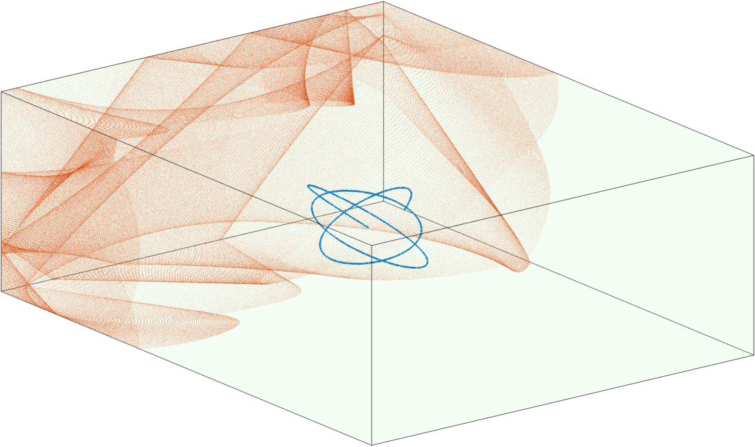
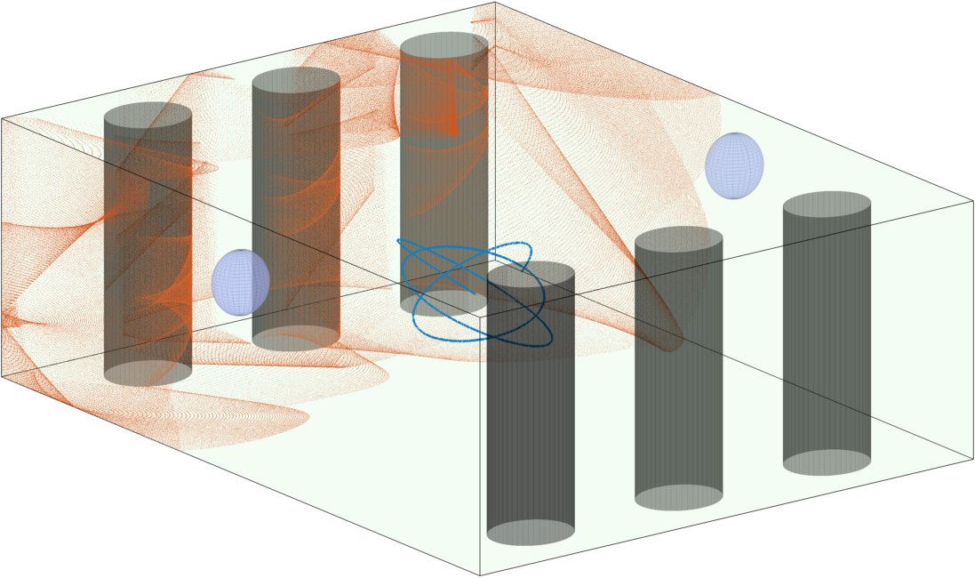
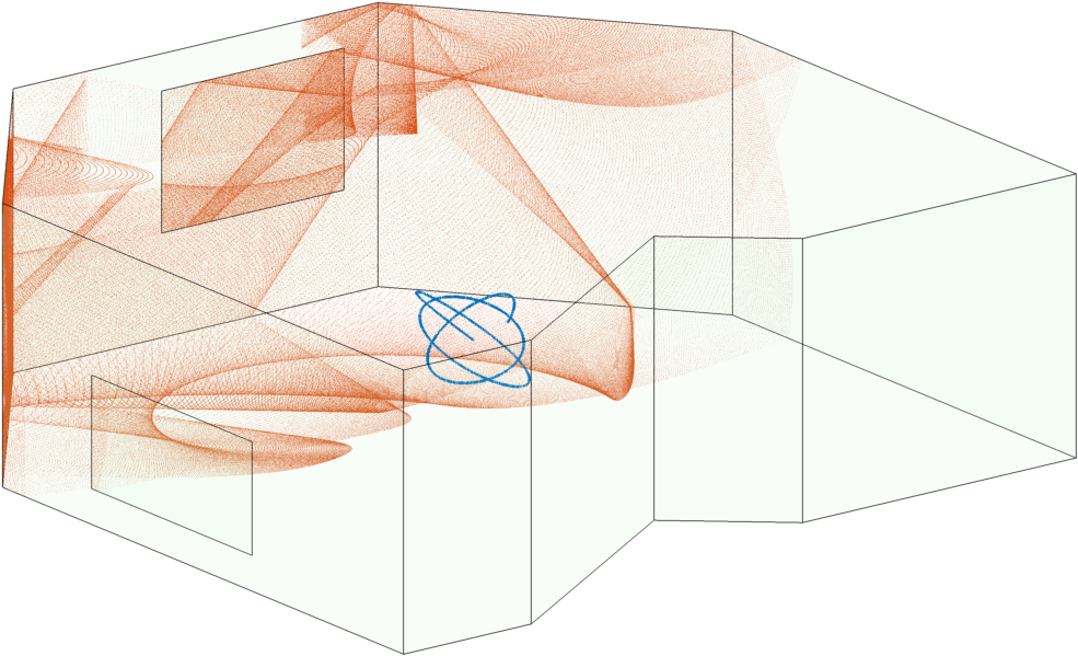
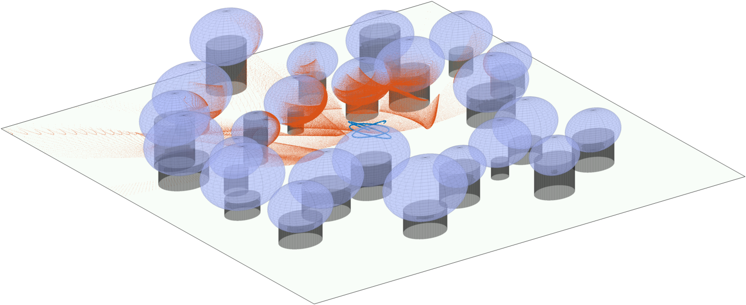
The base sensor trajectories generated for the environments shown in Figure 2 involve sinusoidal motions with unique frequencies and amplitudes for each translational and rotational parameter. A geometrically plausible initial trajectory was determined for each environment, and new trajectories were then produced by randomly varying the frequency and amplitude of each sinusoidal component.

V-B Simulation Environments

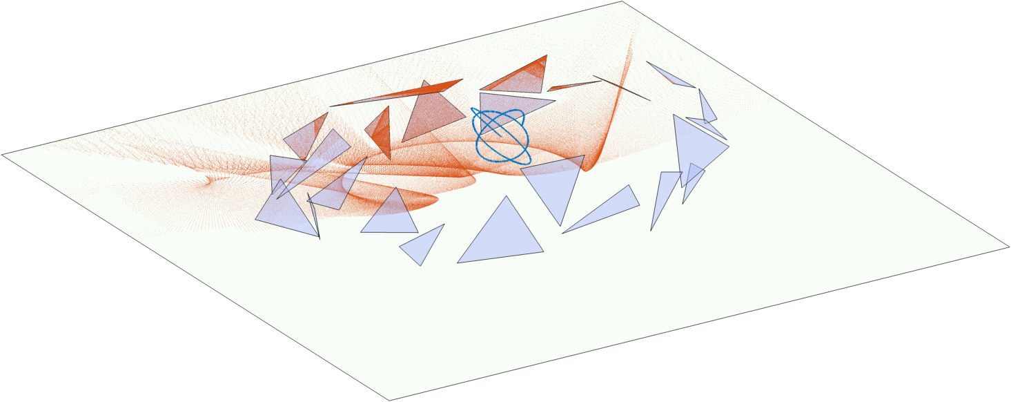
We created five distinct simulation environments, designed to be of increasing difficulty for the algorithm (Figure 2):

1. Simple Room consists only of orthogonal planar surfaces where the sensors move inside an enclosed rectangular ‘room’ (Figure 2(a));

2. Underground Parking Lot adds several pillars (cylinders) to the Simple Room environment (Figure 2(b));

3. Plane City contains planes of varying size, some occluding certain parts of the scene (Figure 2(c));

4. Quadratic Forest is an open environment with spheres mounted on top of cylinders, and where the only planar surface is the ground (Figure 2(d)); and

5. Triangle Array is an open environment filled with non-intersecting triangles of various sizes (Figure 2(e)).

V-C Cost Function Validation

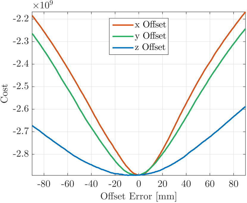
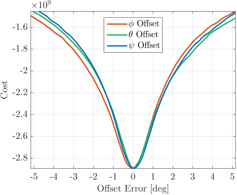
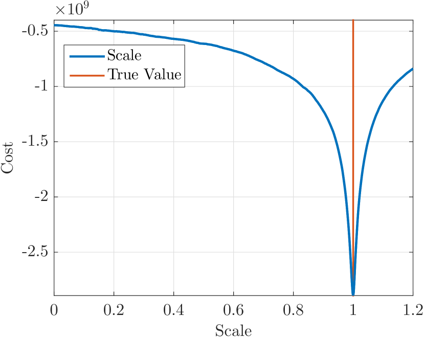
Entropy minimization is an intuitive way to quantify point cloud crispness and therefore extrinsic calibration accuracy, but the measured entropy is dependent on the sensor trajectory and the environment, so it is difficult to derive convergence guarantees for this approach. Instead, we provide experimental validation. While it is difficult to visualize this high dimensional optimization problem, we can gain some insight by varying each parameter individually while holding the other parameters constant. In Figure 3, we see that even with noise, the cost function is minimized very close to the calibration parameters’ true values. This test was performed with the aforementioned noise values in the Simple Room environment. Nevertheless, outside of the region near the true calibration values we have observed that the cost function may not be particularly smooth; we expect the existence of several local minima, increasing the difficulty of the global optimization task.

(a) Offset error versus cost for each translational parameter, with others held constant.

(b) Offset error versus cost for each angular parameter, with others held constant.

(c) Scale parameter versus cost (blue) with true value at scale $=1$ (red), with $SE{3}$ transform parameters held constant.

Figure 3: Effect of variation of individual parameters on cost function, with other parameters held fixed at their true values.

V-D Global Optimization

Table I summarizes calibration accuracy for each parameter in each simulation environment by presenting the average absolute error over 10 randomly generated trajectories. Our method achieves millimetre translational and sub-degree rotational accuracy.

In practice, we found that the base sensor trajectory determined algorithm convergence far more than the environment itself. Some individual runs for the more challenging environments, in particular Quadratic Forest and Triangle Array, produced better results than a typical run in the Simple Room environment. In general, the algorithm converges reliably if the lidar repeatedly scans surfaces from several different viewpoints.

Occasionally, the randomly generated trajectories were identified as degenerate and discarded. We found, in particular, that the roll $\phi$ and yaw $\psi$ parameters were unobservable for several trajectories. We recognize that this is a consequence of our trajectory generation approach, which we intend to improve upon in future work. We posit that the estimation of pitch $\theta$ is a better representation of achievable accuracy of the angular parameter calibration.

V-E Temporal Calibration

Using simulation data, we examined the possibility of adapting our approach for temporal calibration of the sensor data streams, which is often necessary to achieve higher-accuracy results. To this end, we added a 20 ms delay to the lidar scans with respect to the associated camera poses. This represents a worst case scenario based on a state-of-the-art spatiotemporal calibration algorithm [20].

(a) Error in temporal offset between sensors when the Sim(3) transform parameters are held constant at their true values as shown in Table II.

(b) Error in temporal offset between sensors when the Sim(3) transform parameters are held constant at the seed values shown in Table II.

Figure 4: Sample result of the temporal pre-calibration approach, based on a trajectory generated in the Simple Room environment.

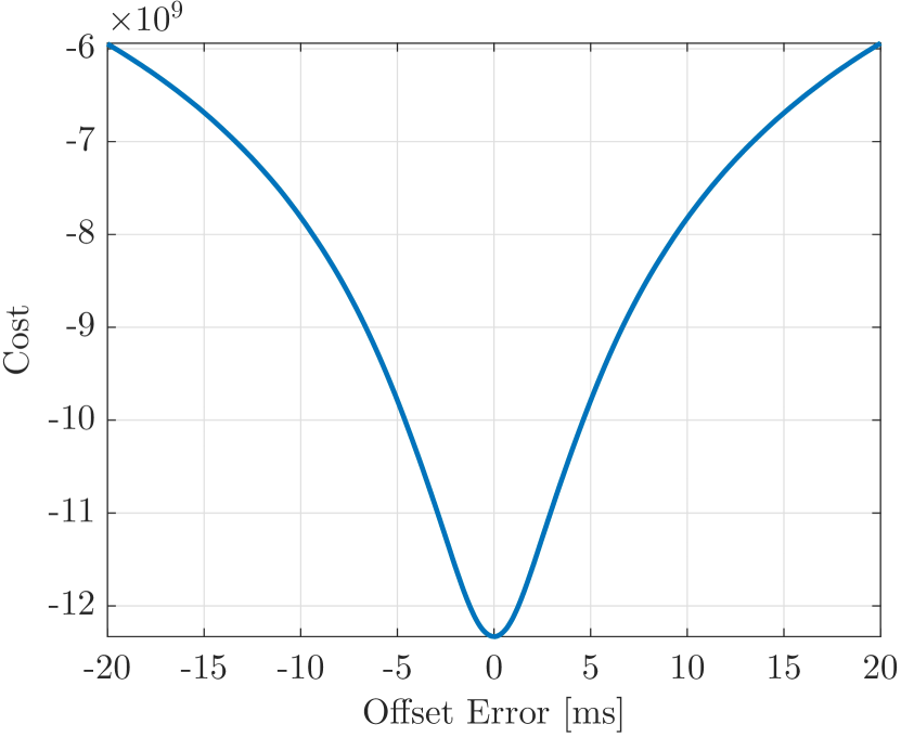
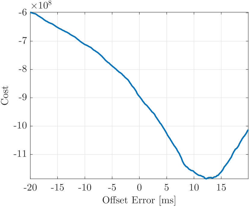
Rather than performing spatial and temporal calibration jointly, we followed [7] and instead attempted to perform temporal calibration prior to spatial calibration, again through entropy minimization (instead of using, e.g., the TICSync library [27]). We locked the Sim(3) transform parameters at nominal values and varied the time delay $t_{d}$ between the camera and lidar data streams, performing a simple linear interpolation between camera poses. Once the optimal value of $t_{d}$ was found, we then held that value constant as we carried out a global optimization over the Sim(3) parameters. A sample result using the true spatial calibration parameters is shown in Figure 4(a), demonstrating that for a noisy trajectory in the Simple Room environment, it is possible to recover the temporal offset exactly.

In realistic scenarios, however, the spatial transform will not be known exactly initially. In Table II, we show the average time offset error after temporal calibration, when the spatial transform parameters are perturbed from their true values. The parameters were seeded $\pm 30$ mm and approximately $\pm 5^{\circ}$ away from ground truth; this represents an initial guess accuracy that should be easily attainable in practice. Figure 4(b) shows how, given a poor initial guess, the estimated time delay between sensors can be inaccurate.

The results presented in Table II indicate how much more difficult point cloud reconstruction becomes when a temporal offset is unaccounted for. Pre-calibrating the time offset is shown to substantially improve the accuracy of the Sim(3) parameter estimates, but the errors remain significantly larger than those in Table I, especially for the angular values. Given the result illustrated by Figure 4(a), we hypothesize that simultaneously estimating the temporal and spatial offset between sensors through entropy minimization could prove to be more reliable than a pre-calibration approach.

TABLE II: Average absolute error on 10 temporally delayed data sets in the Simple Room environment, with and without temporal pre-calibration.

				Average absolute error – $\mu(\sigma)$
Parameter	Initial	True		N.T.C.1	T.C.2
$t_{d}$ [ms]	-	20.0		-	5.6
$x$ [mm]	-230	-200		10.7 (7.8)	3.81 (1.89)
$y$ [mm]	80.0	50.0		7.1 (6.5)	3.0 (2.2)
$z$ [mm]	330	300		18.2 (10.2)	4.9 (3.5)
$\phi$ [deg]	9.74	14.3		0.67 (0.59)	0.39 (0.42)
$\theta$ [deg]	91.7	97.4		0.15 (0.13)	0.10 (0.06)
$\psi$ [deg]	63.0	57.3		0.79 (0.55)	0.47 (0.40)
Scale	1.2	1.0		2.0 (1.2)$\times 10^{-3}$	0.81 (0.52)$\times 10^{-3}$

• Not Temporally Calibrated

• Temporally Calibrated, with average temporal delay ($t_{d}$) value over 10 runs of 14.4 ms (true value was 20 ms).

VI EXPERIMENTS

VI-A Experimental Setup

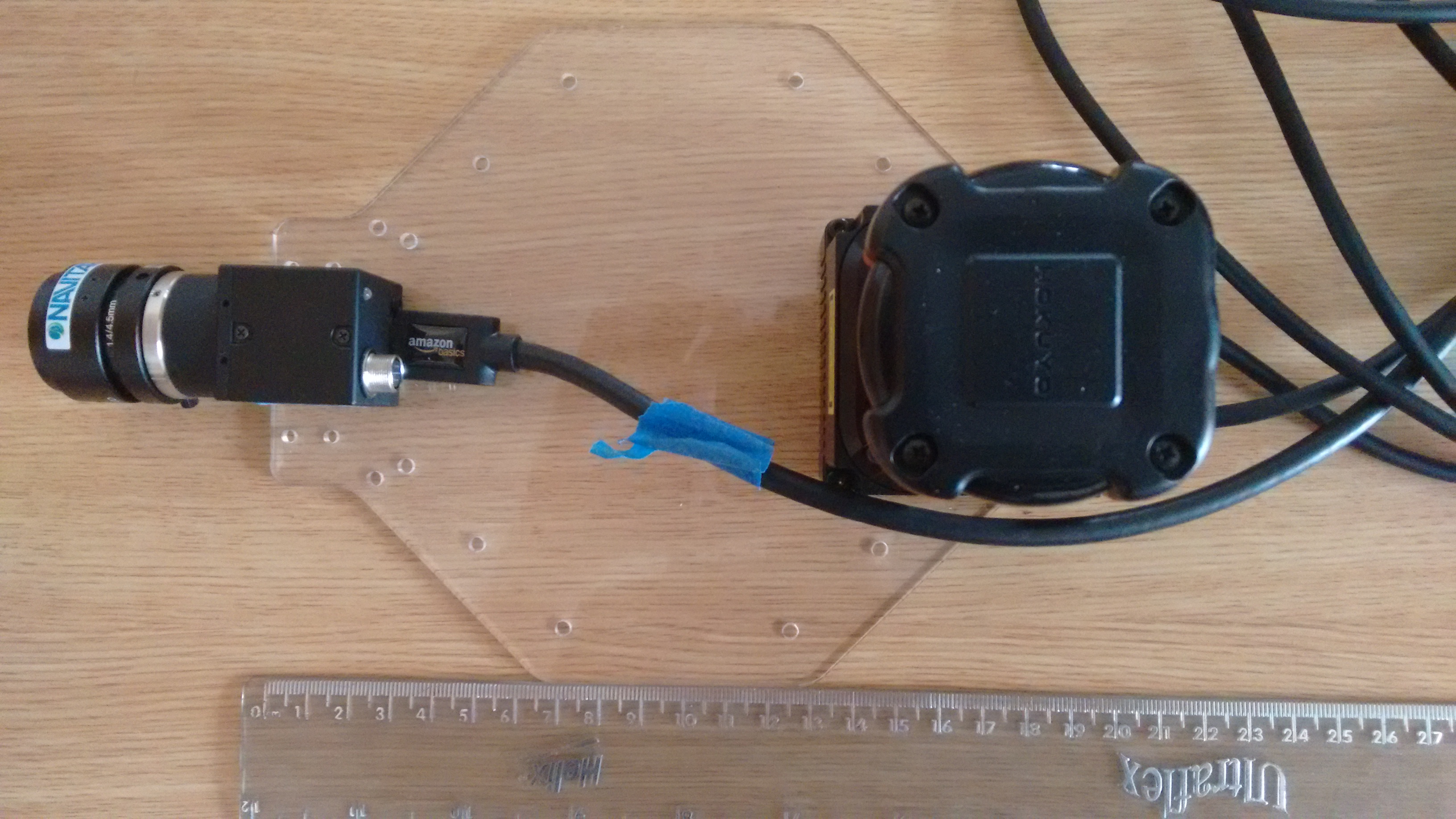
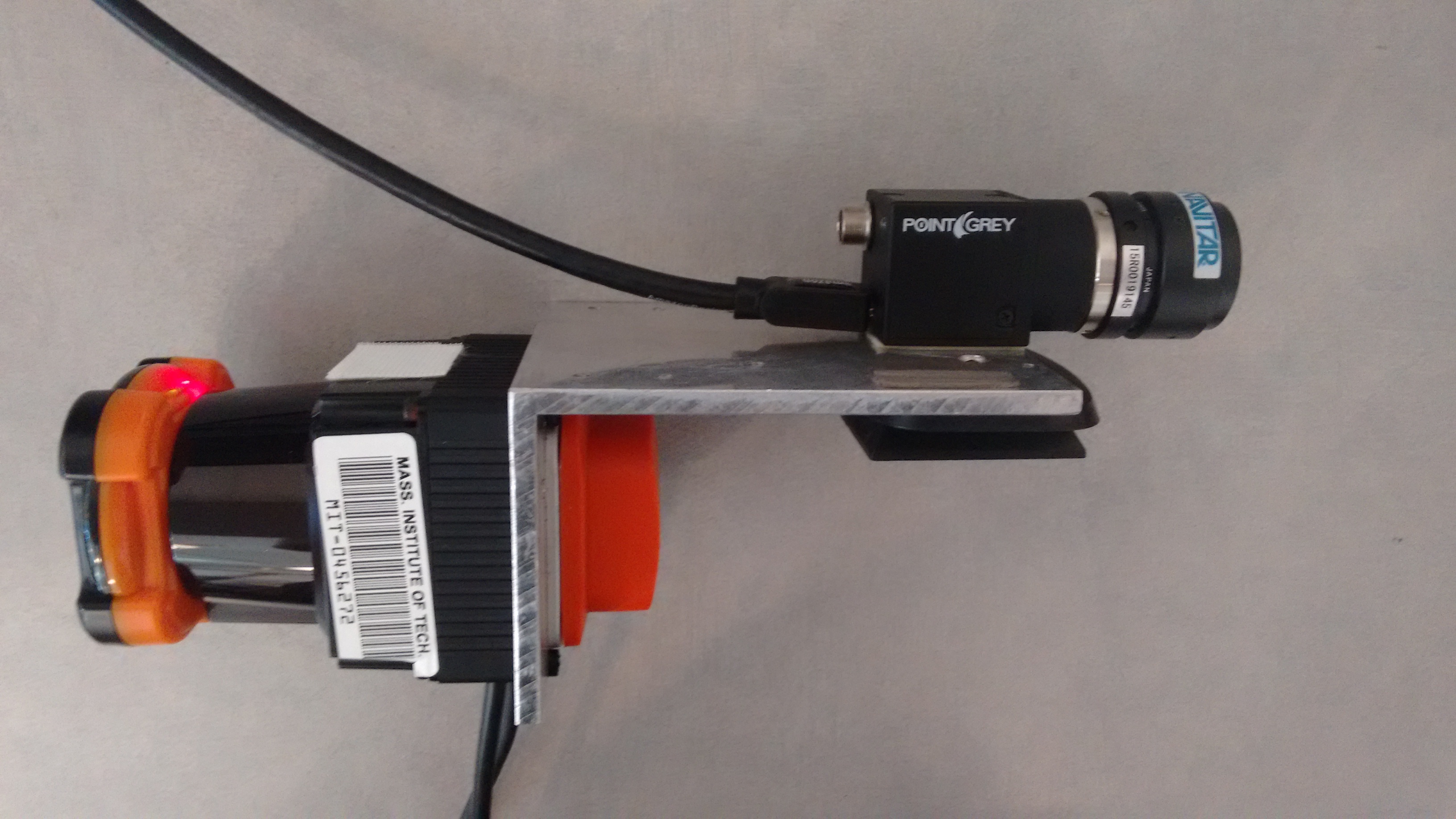
Hardware experiments were conducted with a hand-held sensor rig consisting of a Hokuyo UTM-30LX laser rangefinder and a PointGrey Flea3 monocular camera. The sensors were rigidly fixed to two separate mounts displayed in Figure 5a and Figure 5b. Data were collected via USB on a laptop configured with ROS [28]. All laser data was collected at 40 Hz and 0.25 degree angular resolution, while the camera data was collected at 200 fps with a resolution of 640 $\times$ 512 pixels per frame. We estimated the temporal offset of the lidar relative to the ROS clock using a built-in procedure, then paired the camera and lidar messages according to their timestamps to obtain an approximately synchronized 30 Hz data stream. Given the synchronized data, we estimated the trajectory of the camera (up to an unknown scale factor) using ORB-SLAM2 [23].

(a) Configuration 1: with overlapping sensor FOV.

(b) Configuration 2: non-overlapping sensor FOV.

Figure 5: Hardware configurations used in experiments.

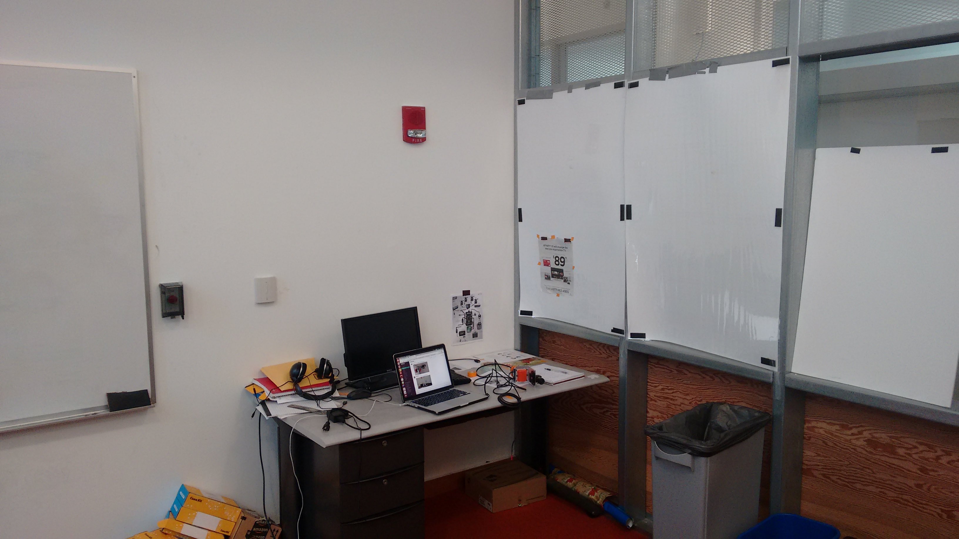
Several data sets were collected in the office space at MIT’s Stata Center, shown in Figure 6. The sensor rig was excited manually, taking care not to capture images or laser measurements of the operator’s body.

Figure 6: Cluttered office space in the MIT’s Stata Center used for data collection.

VI-B Global Optimization

Calibration results are shown in Table III. A data set was collected for each of the sensor configurations shown in Figure 5. Individual data sets contain 2-4 minutes of lidar and camera measurements. To keep the optimization tractable, we split the data sets into segments containing at most 1.9 million lidar points, as in the simulations. For each data set, we initialized the scale parameter by roughly estimating a bounding box around the trajectory during data collection, then comparing with the ORB-SLAM2 trajectory. The scale factor is set based on the choice of keyframes used during ORB-SLAM2 initialization, and hence varies per data set.

TABLE III: Calibration results for the overlapping case, for one data set segmented into four trial runs.

		Calibration results
		$x$ $\left[\mathrm{mm}\right]$	$y$ $\left[\mathrm{mm}\right]$	$z$ $\left[\mathrm{mm}\right]$	$\phi$ [deg]	$\theta$ [deg]	$\psi$ [deg]	Scale $[\times 10^{-3}]$
Initial Guess		$\mathbf{160.0}$	$\mathbf{0.0}$	-$\mathbf{50.0}$	$\mathbf{0.400}$	-$\mathbf{90.00}$	$\mathbf{0.00}$	-$\mathbf{90.00}$
Trial I		-178.2	-3.8	-45.8	90.58	-0.10	-90.74	0.506
Trial II		182.5	-2.8	-50.9	-90.22	0.14	-90.12	0.509
Trial III		173.6	-2.9	-47.8	89.84	-0.27	-90.04	0.506
Trial IV		187.0	-4.9	-54.2	-89.49	-0.02	-90.27	0.511
$\mu$ $\left(\sigma\right)$		180.3 (5.0)	-3.6 (0.8)	-49.7 (3.2)	-90.03 (0.41)	0.06 (0.15)	-90.29 (0.27)	0.508 (0.002)

TABLE IV: Calibration results for the non-overlapping case, for one data set segmented into three trial runs.

		Calibration results
		$x$ $\left[\mathrm{mm}\right]$	$y$ $\left[\mathrm{mm}\right]$	$z$ $\left[\mathrm{mm}\right]$	$\phi$ [deg]	$\theta$ [deg]	$\psi$ [deg]	Scale $[\times 10^{-3}]$
Initial Guess		$\mathbf{50.0}$	$\mathbf{0.0}$	-$\mathbf{250.0}$	$\mathbf{180.00}$	$\mathbf{0.00}$	-$\mathbf{90.00}$	$\mathbf{0.500}$
Trial I		45.2	0.5	-202.1	180.13	-1.11	-88.89	0.2149
Trial II		42.2	-1.2	-202.8	180.73	-1.29	-88.93	0.2159
Trial III		44.0	0.2	-204.2	180.43	-1.78	-88.89	0.2156
$\mu$ $\left(\sigma\right)$		43.8 (1.2)	-0.2 (0.8)	203.0 (0.85)	180.43 (0.24)	-1.39 (0.28)	-88.90 (0.02)	0.2156 (0.0005)

The Sim(3) transform parameters recovered in our experiments are consistent between runs, with very few outliers. We note, however, that the data sets in Table III and IV feature smooth, slow motion in order to minimize the effect of inaccurate temporal calibration, which we found to be critical to obtaining reliable results. Furthermore, the current optimization procedure is computationally expensive for larger data sets, forcing us to significantly reduce the $k$ parameter in Equation 14, and consequently decreasing the accuracy of the cost function[7]. We are actively exploring alternative optimization procedures that would make the computation more tractable, which we believe would lead to more precise results.

VII CONCLUSION AND FUTURE WORK

The automatic approach presented in this paper represents a generalized method for 2D lidar extrinsic calibration. While we focus on 2D lidar to monocular camera calibration, the technique could just as effectively be used to calibrate a 2D, or even 3D lidar to another motion estimation system. GNSS platforms, visual-inertial systems, stereo cameras, and 3D lidars are just a few examples of systems that could make use of the proposed approach—we intend to explore these combinations in future work. The distinct value of this calibration procedure is that it can be performed in virtually any environment, with no limitations on sensor configuration.

We have found in practice that the mis-estimation of the temporal offset between the sensor data streams can severely degrade the quality of the Sim(3) transform parameter estimates. Our temporal pre-calibration approach has limited accuracy, but the results presented in this work motivate the use of RQE minimization in general spatiotemporal calibration.

Finally, we intend to improve the computational tractability of our algorithm to enable online calibration. In particular, we intend to exploit modern GPGPU processing to parallelize the pairwise entropy computations in the cost function, allowing for faster and potentially more accurate calibration.

References

- [1] C. Strecha et al., “Multi-view stereo and lidar for outdoor scene modelling,” Int. Archives of Photogrammetry, Remote Sensing and Spatial Information Science, vol. 36, pp. 19–21, 2007.
- [2] A. Geiger et al., “Vision meets robotics: The KITTI dataset,” Int. J. Robot. Research, vol. 32, no. 11, pp. 1231–1237, Sep. 2013.
- [3] P. Wu et al., “A novel algorithm of autonomous obstacle-avoidance for mobile robot based on lidar data,” in Proc. IEEE Int. Conf. Robot. Biomimetics, Dec. 2015, pp. 2377–2382.
- [4] B. Suger, B. Steder, and W. Burgard, “Traversability analysis for mobile robots in outdoor environments: A semi-supervised learning approach based on 3D-lidar data,” in Proc. IEEE Int. Conf. Robot. Autom., May 2015, pp. 3941–3946.
- [5] O. Miksik et al., “Incremental dense multi-modal 3D scene reconstruction,” in Proc. IEEE/RSJ Int. Conf. Intell. Robot. Syst., Sep. 2015, pp. 908–915.
- [6] B. Jian and B. C. Vemuri, “A robust algorithm for point set registration using mixture of Gaussians,” in Proc. IEEE Int. Conf. Comput. Vision, vol. 2, Oct. 2005, pp. 1246–1251.
- [7] W. Maddern, A. Harrison, and P. Newman, “Lost in translation (and rotation): Fast extrinsic calibration for 2D and 3D LIDARs,” in Proc. IEEE Int. Conf. Robot. Autom., May 2012.
- [8] K. Kwak et al., “Extrinsic calibration of a single line scanning lidar and a camera,” in Proc. IEEE/RSJ Int. Conf. Intell. Robot. Syst., Sep. 2011, pp. 3283–3289.
- [9] O. Naroditsky, A. Patterson, and K. Daniilidis, “Automatic alignment of a camera with a line scan lidar system,” in Proc. IEEE Int. Conf. Robot. Autom., May 2011, pp. 3429–3434.
- [10] C. X. Guo and S. I. Roumeliotis, “An analytical least-squares solution to the line scan lidar-camera extrinsic calibration problem,” in Proc. IEEE Int. Conf. Robot. Autom., May 2013, pp. 2943–2948.
- [11] A. R. Willis, M. J. Zapata, and J. M. Conrad, “A linear method for calibrating LIDAR-and-camera systems,” in Proc. IEEE Int. Symp. on Modeling, Analysis Simulation of Comput. and Telecommun. Syst., Sep. 2009, pp. 1–3.
- [12] A.-I. García-Moreno et al., “LIDAR and panoramic camera extrinsic calibration approach using a pattern plane,” in Proc. Mexican Conf. Pattern Recognition, Jun. 2013, pp. 104–113.
- [13] G. Pandey et al., “Automatic extrinsic calibration of vision and lidar by maximizing mutual information,” J. Field Robot., vol. 32, no. 5, pp. 696–722, 2015.
- [14] Z. Taylor and J. Nieto, “A mutual information approach to automatic calibration of camera and lidar in natural environments,” in Proc. Australasian Conf. Robot. Autom., Dec. 2012.
- [15] H. Yang, X. Liu, and I. Patras, “A simple and effective extrinsic calibration method of a camera and a single line scanning lidar,” in Proc. Int. Conf. Pattern Recognition, Nov. 2012, pp. 1439–1442.
- [16] P. Moghadam, M. Bosse, and R. Zlot, “Line-based extrinsic calibration of range and image sensors,” in Proc. IEEE Int. Conf. Robot. Autom., May 2013, pp. 3685–3691.
- [17] E. Angelats and I. Colomina, “One step mobile mapping laser and camera data orientation and calibration,” Int. Archives of the Photogrammetry, Remote Sens. and Spatial Information Sci., no. 1, pp. 15–20, Mar. 2014.
- [18] Y. Bok, D.-G. Choi, and I. S. Kweon, “Extrinsic calibration of a camera and a 2D laser without overlap,” Robot. and Autonom. Syst., vol. 78, pp. 17–28, Apr. 2016.
- [19] A. Napier, P. Corke, and P. Newman, “Cross-calibration of push-broom 2D lidars and cameras in natural scenes,” in Proc. IEEE Int. Conf. Robot. Autom., May 2013, pp. 3679–3684.
- [20] J. Rehder et al., “Spatio-temporal laser to visual/inertial calibration with applications to hand-held, large scale scanning,” in Proc. IEEE/RSJ Int. Conf. Intell. Robot. Syst., Sep. 2014, pp. 459–465.
- [21] M. Sheehan, A. Harrison, and P. Newman, “Automatic self-calibration of a full field-of-view 3D n-laser scanner,” in Proc. Int. Symp. on Experimental Robot., Dec. 2010.
- [22] J. Brookshire and S. Teller, “Extrinsic calibration from per-sensor egomotion,” in Robotics: Science and Systems VIII, Jul. 2013, pp. 504–512.
- [23] R. Mur-Artal et al., “ORB-SLAM: A Versatile and Accurate Monocular SLAM System,” IEEE Trans. Robot., vol. 31, no. 5, pp. 1147–1163, Sep. 2015.
- [24] A. Rényi, “On measures of entropy and information,” in Proc. Berkeley Symp. Math. Stat. and Probability, vol. 1. University of California Press, 1961, pp. 547–561.
- [25] P. Kaelo and M. M. Ali, “Some variants of the controlled random search algorithm for global optimization,” J. Optimization Theory and Applications, vol. 130, no. 2, pp. 253–264, 2006.
- [26] J. A. Nelder and R. Mead, “A simplex method for function minimization,” Comput. J., vol. 7, no. 4, pp. 308–313, 1965.
- [27] A. Harrison and P. Newman, “TICSync: Knowing when things happened,” in Proc. IEEE Int. Conf. Robot. Autom., May 2011, 05.
- [28] M. Quigley et al., “ROS: An open-source robot operating system,” in Proc. IEEE Int. Conf. Robot. Autom. Workshop on Open Source Software, vol. 3.