Gerrymandering and the net number of US House seats won due to vote-distribution asymmetries

Abstract

Using the recently introduced declination function, we estimate the net number of seats won in the US House of Representatives due to asymmetries in vote distributions. Such asymmetries can arise from combinations of partisan gerrymandering and inherent geographic advantage. Our estimates show significant biases in favor of the Democrats prior to the mid 1990s and significant biases in favor of Republicans since then. We find net differences of 28, 20 and 25 seats in favor of the Republicans in the years 2012, 2014 and 2016, respectively. The validity of our results is supported by the technique of simulated packing and cracking. We also use this technique to show that the presidential-vote logistic regression model is insensitive to the packing and cracking by which partisan gerrymanders are achieved.

1 Introduction

The partisan composition of the US House of Representatives is the result of a number of factors: the economy, social issues, who is president, party platforms, voter ID laws, propaganda, campaign finance laws, the characteristics and incumbency statuses of individual candidates, and district plans, to name a few. Our focus in this paper is on district plans.

A partisan gerrymander is, by definition, a district plan that enables a party to win more seats than it would have under a “neutral” district plan. It is sometimes easy to detect a partisan gerrymander. For example, a North Carolina legislator openly admitted that his committee planned to redraw districts with a goal of partisan advantage [Gan16]. Other times the convoluted shapes of districts provide evidence that is almost as compelling. In fact, significant energy has been devoted to developing geometric methods of identifying gerrymandered districts (see [NGCH90] for an overview). But none of these geometric approaches provide a direct way to determine the number of extra seats that have been won through the gerrymander — the fundamental purpose of a partisan gerrymander.

In the first part of this paper we use the declination function, $\delta$, introduced by the second author in [War17], to estimate the effect of asymmetries in how district plans treat the two major parties on the number of House seats won by each. To do so, we explore more thoroughly the scaled function $5N\delta/12$ which we refer to in this paper as the $S$-declination. (The variable, $N$, denotes the number of districts in the election; “$S$” is intended to remind the reader that this scaling counts seats.) We argue that the $S$-declination provides a good estimate of the number of extra seats won through these partisan asymmetries.

Remark 1.

In [War17] we consider a similar scaling of $N\delta/2$. While simpler, this appears to slightly overcount the number of seats in a given state and year. The effect is not significant when single-state US House elections are considered as is done in [War17], but in the typically larger state legislatures or when considering national effects, the difference between the two scalars is non-trivial.

Table 1 presents the results of applying the $S$-declination to the US House elections since 1972. The data indicate that, on a national level, while the Democrats consistently benefited through the early 1990s from partisan asymmetry in district plans, the situation has been reversed since the late 1990s.

There have been a number of previous attempts to estimate the net effect of gerrymandering on a national level (see, e.g., the references in [CC16]). The most recent of which we are aware is a report [RL17] by Royden and Li that considers House elections since 2012. Our estimate for the year 2012 of 28 extra republican seats falls within 25–36, the narrower of the two ranges provided by Royden and Li. However, our estimate differs markedly from the estimate of approximately one seat arrived at in a recent paper [CC16] by Chen and Cottrell. (See also, [Wan16, pgs. 36,37] whose results are intermediate to those of the mentioned studies.)

In the second part of this paper we attempt to explain the discrepancy between the Chen-Cottrell estimate and the two other estimates. Our main tool will be a simulated packing and cracking technique that we introduce in Section 2. We first use this technique to validate the $S$-declination as a means of counting extra seats. We then use it to show that the logistic-regression approach of Chen and Cottrell is insensitive to the main technique of partisan gerrymandering.

The structure of this paper is as follows. In Section 2 we introduce the necessary background and terminology on both partisan gerrymandering as well as on packing and cracking. We also describe a simple framework for simulated packing and cracking that we use in later sections to gauge how faithfully various methods register partisan gerrymandering efforts. In Section 3 we review the declination function and show using the packing and cracking technique that the declination faithfully registers partisan gerrymandering. In Table 1 we record the net number of seats in House elections since 1972 that, according to the declination, should be attributed to partisan asymmetry in the vote distribution. In Section 4 we show that the model utilized in [CC16] is insensitive to packing and cracking, thereby explaining the discrepancy between their estimate and the estimates of both this paper and [RL17]. We end with our conclusion.

2 Background

Partisan gerrymanders have historically been recognized by identifying individual districts with contorted boundaries. The primary advantage of this approach is that wild shapes are immediately convincing as evidence of nefariousness. Unfortunately, there are several disadvantages. First, there are many valid reasons for a district to have a strange shape (e.g., geographic constraints, the Voting Rights Act, and county boundaries). Second, gerrymandering can occur without particularly unusual boundaries. Third, the shapes of the districts do not directly tell one anything about how effective the gerrymander is in winning additional seats for one party. An alternative approach to the study of district shapes is to analyze the distribution of votes among the various districts. In this section we introduce the notation and terminology necessary to work with these distributions and to see the effect partisan gerrymandering has on them. We assume that each district has the same number of total votes.

We define an $N$-district election to be a weakly increasing sequence $\boldsymbol{\ell}=(\ell_{1},\ell_{2},\ldots,\ell_{N})$ in which $\ell_{i}$ indicates the democratic fraction of the two-party (legislative) vote in district $i$. We visualize $\boldsymbol{\ell}$ by plotting a point $v_{i}=(i/N-1/2N,\ell_{i})$ for each $i$. Figure 1 illustrates plots of $\boldsymbol{\ell}$ for three hypothetical elections.

Figure 1: Symmetric vote distributions for fair elections with equally popular parties.

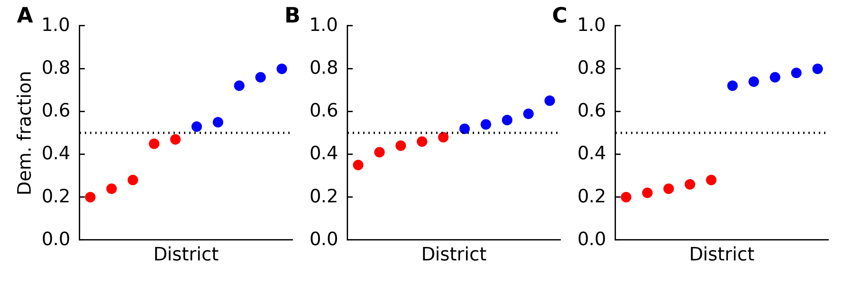
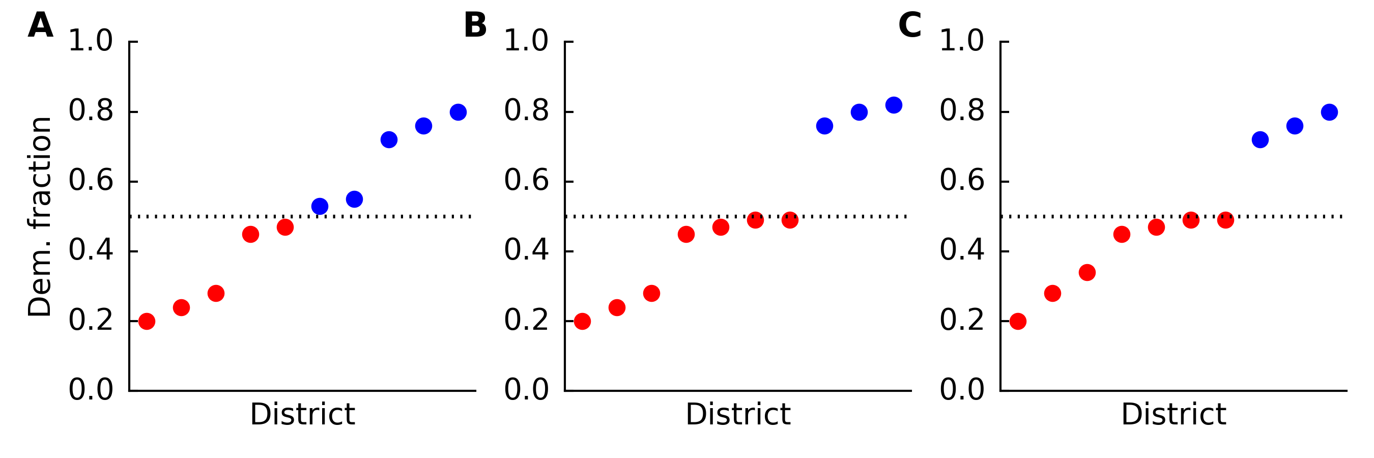
While researchers are still working on robust tests both for identifying gerrymanders and for assessing the effects of gerrymandering, how partisan gerrymandering occurs is well understood: Parties create partisan gerrymanders by “packing and cracking” votes. Suppose the Democrats are in control of redistricting and the Republicans are poised to win district $X$. In packing, Republicans are moved from $X$ to other districts in which the Republicans already have enough strength to win. These votes are effectively wasted in the new districts while district $X$ falls to the Democrats. Cracking works similarly, except now the Republicans are spread among districts that they have no chance of winning. Once the cracking occurs, the recipient districts are lost by the Republicans by smaller margins, but they are still lost. Figure 2 illustrates the effect of packing and cracking on the vote distribution illustrated in Figure 1.A.

Figure 2: (A) Repeat of election from Figure 1.A. (B) Illustration of packing of the distribution from (A) for a gain of two republican seats. (C) Illustration of cracking of the distribution from (A) for a gain of two republican seats.

2.1 Simulated packing and cracking

In order to validate the $S$-declination (see Section 3) as a measure of the number of extra seats won under a partisan gerrymander, we will examine how perturbations of a vote distribution by packing and/or cracking affect the value of the $S$-declination. The simple technique we will use is that of simulated packing and cracking (SPC). In short, we manually modify a vote distribution by packing or cracking so as to flip a single district from one party to the other. There are four possible composite choices: whether we are packing or cracking and whether it is the Republicans or the Democrats who are in charge of the gerrymander. In reality, the votes from the flipped district could be distributed among other districts by a combination of packing and cracking, but we do not attempt to model this. We focus below on the case in which the Republicans are flipping a single democratic district to republican control using cracking. The other three cases are treated similarly.

In practice, the details of a gerrymander will depend on many factors. One such factor will be the geography of the state. If a given district is being cracked so as to turn it from a democratic district to a republican district, the surplus democratic voters will have to be allocated to adjacent districts. Of course, this process can be iterated by swapping other democratic voters for republican voters in second-order neighbors of the original district. Nonetheless, there are obvious geographic constraints that may be significant. Another factor is how risk averse the gerrymandering party is. For example, if the Democrats wish to maximize their potential gain in seats (albeit at a high risk of the plan backfiring) they can crack republican districts by creating districts that are (say) 49% republican. On the other hand, if the Democrats feel the political winds will be against them in the upcoming decade, they may prefer to pack Republicans into districts so that the democratic districts are no more than (say) 35% republican.

For our model, we make the following conventions for how the gerrymander is achieved.

1. The flipped district is the democratic district that is won by the narrowest margin.

2. The gerrymander does not create any new republican-majority districts with a democratic vote fraction of greater than $0.45$. We choose this value on the basis that a 45–55 split is frequently considered the threshold for a race to be competitive (see, for example, [AAG06]). Any republican-majority district with a democratic vote fraction higher than this before the cracking is allowed to remain at such a level.

3. The modified democratic vote fraction in the flipped district is chosen according to a linear regression of the democratic vote fractions among the republican districts. If the linear regression yields a new democratic vote fraction in the flipped district greater than $0.45$, then the value is set to exactly $0.45$.

4. The democratic votes shifted from the flipped district are distributed evenly among the republican-majority districts with a democratic vote fraction of at most $0.45$. In order to avoid violating the second convention, this process may need to be iterated (see Example 2 below).

In order to illustrate the method in practice we present the following example of flipping a district from democratic to republican by cracking. While we use hypothetical data in this example, all subsequent applications of simulated packing and cracking in this paper involve vote distributions from actual elections.

Example 2.

Consider a $10$-district election

$$\boldsymbol{\ell}=(0.37,0.40,0.43,0.46,0.60,0.63,0.66,0.69,0.72,0.75).$$

By Convention 1, we flip the fifth district. A linear regression of the four points

$$\left\{\frac{i}{10}-\frac{1}{2\cdot 10},\ell_{i}\right\}_{i=1}^{4}=\{(0.05,0.37),(0.15,0.40),(0.25,0.43),(0.35,0.46)\}$$

yields a line with intercept $0.355$ and slope $0.3$. Thus, according to the linear regression line, the flipped district should be switched from a democratic vote fraction of $0.6$ to one of $0.49$. However, by Convention 3 we instead choose a value of $0.45$. In order to maintain the same statewide democratic vote fraction, there must be a net increase of $0.15$ among the first three districts (note that the fourth district is not included since its democratic vote fraction already exceeds $0.45$). Convention 4 instructs us to distribute these democratic votes evenly among the three districts. The resulting vote distribution is

$$(0.42,0.45,0.48,0.46,0.45,0.63,0.66,0.69,0.72,0.75).$$

However, following Convention 4, we iterate the process by redistributing the excess fraction of $0.03=0.48-0.45$ from the third district evenly among the first two districts. Since the second district is already at a value of $0.45$, the amount is entirely distributed to the first district. This yields a final vote distribution of

$$\boldsymbol{\ell}^{*}=(0.45,0.45,0.45,0.46,0.45,0.63,0.66,0.69,0.72,0.75).$$

We utilize SPC for two purposes in this paper. In each instance, we analyze a vote distribution using some function both before and after the SPC. We have rerun the analyses in this paper with different values of the maximum democratic vote fraction equal to $0.40$ and $0.49$. We have also analyzed the effect of a “greedy” distribution of votes in which the extra votes from the flipped district are distributed to the districts whose democratic and republican votes are distributed most unevenly. The resulting data and figures corresponding to Figures 4, 6 and 8 are qualitatively very similar.

3 The declination

The declination function was introduced in [War17] as a way of identifying potential gerrymanders by quantifying partisan asymmetry in the vote distribution. A number of other vote-distribution functions created for this purpose can be found in the literature (several of these are mentioned in Section 4).

The declination is based on two observations. The first is that a constitutionally manageable standard for partisan gerrymandering could conceivably be based on some measure of partisan asymmetry, that is, a measure of how the district plan treats the parties differently. The second observation, which we make in [War17], is that there should be nothing special about the 50% vote threshold in individual districts. Combining these observations leads us to compute the ratio of “average winning margin” to “fraction of seats won” for each party. The declination is simply a comparison of these two ratios. If the 50% threshold is truly not special, then the resulting ratios for each party should be approximately equal. The declination can be computed geometrically as follows (see [War17] for details).

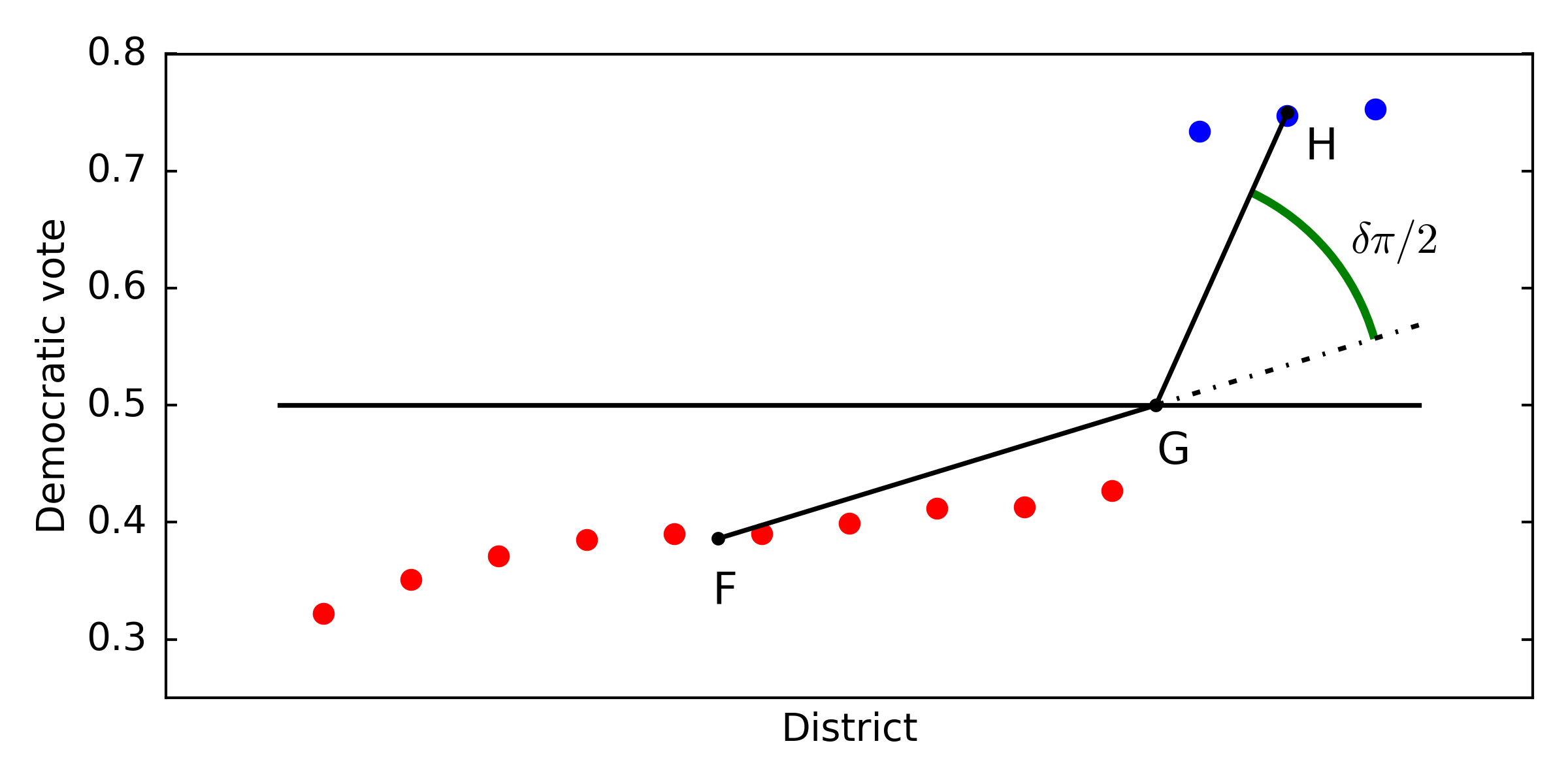
Let $v_{i}$ denote the point $(i/N-1/2N,\ell_{i})$ for each $1\leq i\leq N$. Place a point $F$ at the center of mass of the points $v_{i}$ corresponding to the districts the Democrats lose; a point $H$ at the center of mass of the points $v_{i}$ the Democrats win; and a third point $G$ at $(k/N,1/2)$, where $k$ is the number of districts the Democrats lose. See Figure 3.

If the district plan treats the parties symmetrically, we would expect the point $G$ to lie on the line $\overline{FH}$. As such we define the declination, $\delta$, to be $2/\pi$ times the angle between the lines $\overline{FG}$ and $\overline{GH}$ (using the convention that a counterclockwise angle from $\overline{FG}$ to $\overline{GH}$ is measured positively). Multiplication by $2/\pi$ converts from radians to fractions of $90$ degrees. Therefore, possible values of the declination are between $-1$ and $1$. Positive values indicate a republican advantage while negative values indicate a democratic advantage.

Figure 3: Illustration of the two lines $\overline{FG}$ and $\overline{GH}$ arising in the definition of the declination, $\delta$, for the $13$-district 2014 North Carolina congressional election. Districts have been sorted in increasing order of democratic vote share. The value of $\delta$ is approximately $0.54$ in this case.

3.1 The $S$-declination

The declination metric was introduced for the purpose of measuring the degree to which district plans result in partisan asymmetry in the vote distribution. It is essentially an angle associated to each election and it is not obvious that it can be used to provide a good estimate of how many extra seats have been won due to the asymmetry. While the declination itself does not count seats, we propose that the $S$-declination, which we set equal to $5N\delta/12$, does.

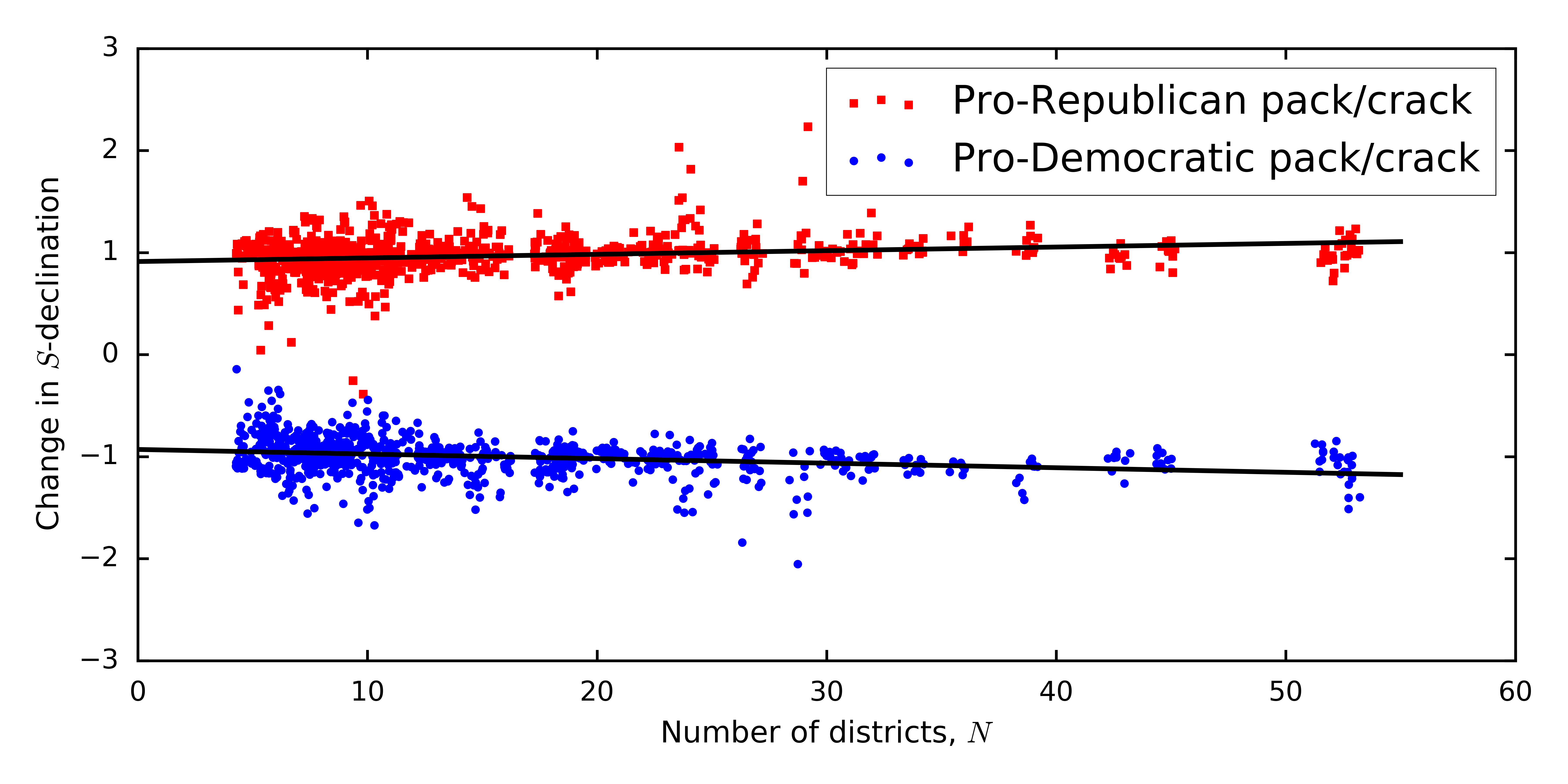
To support this claim we use SPC on the vote distributions from a number of elections and examine the effect on the $S$-declination. If the distribution is modified by flipping one district from democratic to republican through packing or cracking, the $S$-declination should increase by about one. If the flip is from republican to democratic, it should decrease by about one. To this end, we consider the data set from [War17] consisting of all state-wide elections to the US House of Representatives in presidential-election years since 1972. (Note that a multilevel model is used in [War17] to impute the democratic vote fraction for uncontested elections.) For any such election we can attempt to pack or crack it in favor of either party. In Figure 4 we illustrate the change in $S$-declination for those instances in which the SPC is successful.

The instances of SPC plotted in Figure 4 are restricted in two ways. First, we require that each party win at least one seat both before and after the packing/cracking. This is necessary for the $S$-declination of each distribution to be defined. Second, we require that there be at least three districts into which to distribute the votes from the flipped district. For example, when a seat is being flipped from democratic to republican by cracking, we require that there be at least three republican seats in the original distribution. Together, these restrictions exclude states in which there are four or fewer congressional districts. In the current apportionment cycle there are 21 such states:

$$\text{AK, AR, DE, HI, IA, ID, KS, ME, MS, MT, ND,}\\ \text{NE, NH, NM, NV, RI, SD, UT, VT, WV, and WY.}$$

There were 352 state-year pairs in which there were at least five districts and each party won at least one seat. Given the four possible combinations of packing/cracking and pro-republican/pro-democratic, this offers 1408 possible applications of SPC. However, for 415 of these, either there was not enough room for the chosen packing/cracking or one of the constraints was not satisfied.

When flipping a seat from democratic to republican, we find that 95% of the time the $S$-declination changes by an amount between $0.69$ and $1.20$. For a flip from republican to democratic, the corresponding range is $-1.26$ to $-0.74$. We conclude that the declination is a reasonably good recorder of packing and cracking.

We estimate how many net seats have been won in each year on the basis of partisan asymmetry in the vote distribution as follows: For a given year add together the values of the $S$-declination (rounded to the nearest integer) for each state. The results are shown in Table 1. Unfortunately, the $S$-declination simply provides an estimate without error bounds. Note that a given state-year does not contribute to the sum from that year if one party wins all of the seats in the state that year. However, we do not place the additional constraints used for the generation of Figure 4 as the values in Table 1 rely only on actual vote distributions and not on values derived from SPC.

Figure 4: Plot of change in the $S$-declination due to SPC. Red squares indicate the 502 ways in which presidential-year House elections since 1972 can be packed/cracked so that the Republicans win one more seat, subject to the constraints noted in the main text; blue circles indicate the 491 corresponding ways in which presidential-year elections since 1972 can be packed/cracked so that the Democrats won one more seat. Note that horizontal coordinates have been jittered for clarity. The linear regression lines are $0.908+0.004N$ ($r^{2}=0.05$, $\mathrm{RMSE}=0.17$) and $-0.9305-0.004N$ ($r^{2}=0.09$, $\mathrm{RMSE}=0.16$), respectively.

Table 1: Net effect of vote-distribution asymmetry on partisan composition of House as determined by $S$-declination. Positive (negative) values indicate a benefit to Republicans (Democrats).

Year	Seats	Year	Seats	Year	Seats	Year	Seats	Year	Seats
1972	-1	1982	-16	1992	-7	2002	5	2012	28
1974	-2	1984	-20	1994	0	2004	20	2014	20
1976	-23	1986	-10	1996	12	2006	20	2016	25
1978	-28	1988	-19	1998	9	2008	7
1980	-10	1990	-12	2000	13	2010	17

4 Two recent studies

We now turn our attention to two recent studies that have also attempted to answer the question of the net result of gerrymandering in the House.

4.1 Royden and Li study

The most recent study, a Brennan Center [RL17] report by Royden and Li, considers House elections since 2012. The authors’ approach is to use functions (akin to the declination) that identify gerrymanders by quantifying asymmetries in the vote distribution among districts. They consider three such functions from the literature: the efficiency gap [McG14, MS15], the seats-votes curve [MSK15] and the median-mean difference [KMM⁺16, MB15, Wan16]. The first two of these functions are able to provide estimates of the number of seats won as a result of gerrymandering. For the 2012 congressional elections, these functions both come to very similar conclusions: the Republicans gained between 25 and 37 extra seats. The estimate from Table 1 falls at the lower end of this range. An important caveat to their methodology is that it does not account for any inherent democratic disadvantage owing to geographic clustering. This is true of the declination as well. However, the authors find a high correlation between states with single-party redistricting control and large numbers of extra seats, thereby suggesting that geography fails to account for a significant portion of the asymmetry.

4.2 Chen and Cottrell study

In [CC16], Chen and Cottrell take what is perhaps a more intuitive approach to evaluating the net effect of gerrymandering. For each state, they use 200 computer-generated “neutral” district plans as a standard to which the results of the enacted district plan are compared. Utilizing aggregated precinct-level presidential vote data, they estimate the probability that each simulated district in each simulated plan elects a democratic representative. These probabilities, over all districts, immediately yield an expected number of democratic representatives in the House under each such simulated district plan. They find that the expected number of democratic seats in the enacted plans is only one less than the average of the expected number of seats in the simulated plans, leading them to conclude that the net effect of gerrymandering in the House is trivial. Note that a putative advantage is that by incorporating the geographic distribution of voters, this approach has the potential to account for geographic clustering.

Remark 3.

Choosing simulated district plans from an appropriate distribution is a notoriously difficult problem that is not even well defined. Issues one must contend with include how to deal with constraints imposed by the Voting Rights Act; how to recognize communities of interest; the extent to which one should respect existing political boundaries; how to define compactness; how strict compactness constraints should be made; and how to weigh all of these disparate factors. Even once one makes such decisions, it is not necessarily clear how one chooses uniformly from the space of remaining “acceptable” district plans. Finally, there remains the nebulous problem of how to relate the choices made to what human map drawers do, or should be doing, when they create maps. We do not address these issues as they arise in [CC16] as they are nuanced and beyond the scope of this paper.

The declination discussed in Section 3 and the functions utilized by Royden and Li directly count extra seats won as a result of partisan asymmetry in the vote distribution. However imperfect these measures may be, we have no more logically direct way to count such seats. As mentioned above, the approach of Chen and Cottrell has the advantage that it more directly addresses inherent geographic advantages. However, while this approach should, a priori, be able to count extra seats, the connection is less direct. In the remainder of this section we argue, in fact, that the logistic regression model used fails to capture gerrymandering to any appreciable degree. In the computations that follow, we will omit uncontested districts: Our goal is not to accurately estimate the exact number of seats a given party would win, but simply to see how the estimate changes under SPC.

We now present the notation required for the model. Let $p_{i}$ denote the presidential vote in district $i$. Following Chen and Cottrell, we consider a simple logistic-regression model for estimating the expected number of democratic seats won in district $i$ as a function of $p_{i}$. According to their logistic model, the expected number of democratic seats in district $i$ is $F(\beta_{0}+\beta_{1}p_{i})$ where $F(x)=(1+e^{-x})^{-1}$ and $(\beta_{0},\beta_{1})$ are regression coefficients that are estimated from the data. For an election with presidential vote $\boldsymbol{p}=(p_{1},p_{2},\ldots,p_{N})$, the expected number of democratic seats is then

$$E(\boldsymbol{p})=\sum_{i=1}^{N}F(\beta_{0}+\beta_{1}p_{i}).$$ (1)

Chen and Cottrell used presidential data from 2008 and 2012 along with the four House elections from 2006 to 2012 to estimate the parameters $\beta_{0}$ and $\beta_{1}$. In order to use election data from 1972 to 2012, we replaced $\beta_{0}$ and $\beta_{1}$ with random year effects $\beta_{0[j]}$ and $\beta_{1[j]}$ with $j$ indexing the year. Under this model (suppressing the dependence of $E(\boldsymbol{p})$ on $j$), the expected number of democratic seats becomes

$$E(\boldsymbol{p})=\sum_{i=1}^{N}F(\beta_{0[j]}+\beta_{1[j]}p_{i}).$$ (2)

Estimates of the intercept and slope parameters $\beta_{0[j]}$ and $\beta_{1[j]}$ using maximum likelihood are listed in Table 2.

Our approach to analyzing this model is analogous to our validation of the $S$-declination: We apply SPC to historical vote distributions and observe the effect on the predicted number of seats each party will win. However, there is an added complication. When packing and cracking, the vote of greatest interest in district $i$ is not the presidential vote $p_{i}$, but the legislative vote $\ell_{i}$. Unfortunately, SPC provides us only with a modified legislative vote. We will need a mechanism for estimating district-level presidential votes from district-level legislative votes.

Figure 5: Plot of legislative vote $\boldsymbol{\ell}^{\circ}$ versus presidential vote $\boldsymbol{p}^{\circ}$. Races are colored according to incumbency statuses of the candidates: democratic incumbent (blue); republican incumbent (red); no incumbent or two incumbents from opposite parties (gray). Regression lines are also plotted. (A) Presidential-year elections from 1972–2012: intercept $0.22$, slope $0.51$, $r^{2}=0.42$; (B) 1980 election: intercept $0.23$, slope $0.43$, $r^{2}=0.44$; (C) 2012 election: intercept $0.08$, slope $0.85$, $r^{2}=0.91$.

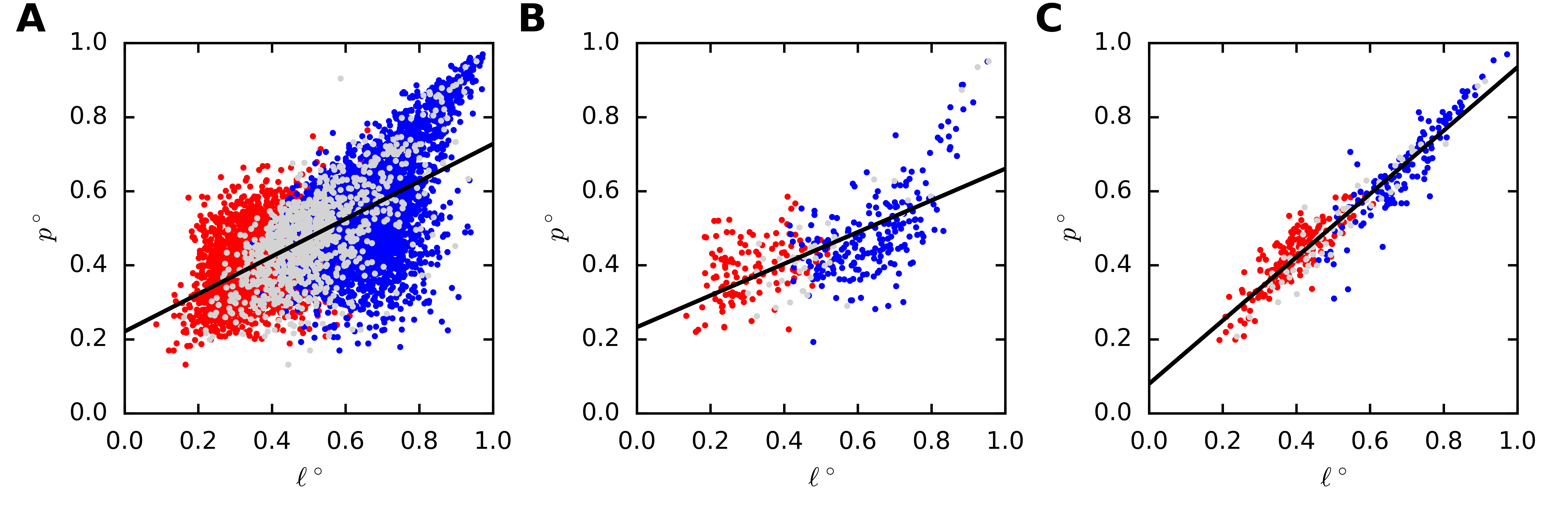
If $p_{i}$ and $\ell_{i}$ directly determined each other, there would be no need for a logistic regression in (1). You would be able to determine who won the seat from the value of $p_{i}$ without any appeal to probability. As shown in Figure 5 (see also Table 2), there is some justification for asserting a linear relation between the presidential vote and the legislative vote. (This relation is certainly much stronger in some years than others.) One could also choose to fit the three subsets corresponding to elections in which there is a democratic incumbent, a republican incumbent, or no incumbent, however we do not pursue this variation.

In the remainder of this subsection we will model $p_{i}$ as a linear function, $g$, of $\ell_{i}$. Letting $j$ index the year, we set $p_{i}=g(\ell_{i}):=\gamma_{0[j]}+\gamma_{1[j]}\ell_{i}$ for some coefficients $\gamma_{0[j]}$ and $\gamma_{1[j]}$. The function $g$ is dependent on the year $j$, however we will suppress this from the notation. For the remainder of this section we will reserve $\boldsymbol{p}^{\circ}=(p^{\circ}_{1},\ldots,p^{\circ}_{N})$ and $\boldsymbol{\ell}^{\circ}=(\ell^{\circ}_{1},\ldots,\ell^{\circ}_{N})$ for the historical values given to us in our data set. We reserve $\boldsymbol{\ell}^{*}=(\ell^{*}_{1},\ldots,\ell^{*}_{N})$ for the legislative vote after applying one of the four variations of SPC to $\boldsymbol{\ell}^{\circ}$. The presidential vote associated to $\ell^{*}_{i}$ will be written $p^{*}_{i}=g(\ell^{*}_{i})$. (Note, however, that $g(\ell^{\circ}_{i})$ does not equal $p^{\circ}_{i}$.)

4.2.1 The simplest model: $\gamma_{0[j]}=0$, $\gamma_{1[j]}=1$ for all $j$.

We begin with the simplest reasonable parameters: $\gamma_{0[j]}=0$ and $\gamma_{1[j]}=1$ for all $j$. While there are a number of obvious objections to assuming the presidential and legislative votes are equal, there are reasons to believe that it is a best-case scenario for the Chen-Cottrell approach. That is, if their approach does not record SPC under this model, then it will not do so under a more tenuous relation between the two votes. Since $E(g(\boldsymbol{\ell}^{\circ}))$ is the expected number of democratic seats initially, $E(g(\boldsymbol{\ell}^{*}))-E(g(\boldsymbol{\ell}^{\circ}))$ is the change in the expected number of democratic seats after SPC. In Figure 4, a vertical coordinate of $1$ indicates one more seat for the Republicans. For consistency, therefore, we consider the negative, $E(g(\boldsymbol{\ell}^{\circ})))-E(g(\boldsymbol{\ell}^{*}))$, the expected change in the number of republican seats. By (2) and our choice of $\gamma_{0[j]}=0$, $\gamma_{1[j]}=1$, we then have that the expected change in republican seats is given by

$$E(g(\boldsymbol{\ell}^{\circ}))-E(g(\boldsymbol{\ell}^{*})) =\sum_{i=1}^{N}[F(\beta_{0[j]}+\beta_{1[j]}g(\boldsymbol{\ell}^{\circ})_{i})-F(\beta_{0[j]}+\beta_{1[j]}g(\boldsymbol{\ell}^{*})_{i})]$$ (3)

$$=\sum_{i=1}^{N}[F(\beta_{0[j]}+\beta_{1[j]}(0+1\cdot\ell^{\circ}_{i})-F(\beta_{0[j]}+\beta_{1[j]}(0+1\cdot\ell^{*}_{i})]$$

$$=\sum_{i=1}^{N}[F(\beta_{0[j]}+\beta_{1[j]}\ell^{\circ}_{i})-F(\beta_{0[j]}+\beta_{1[j]}\ell^{*}_{i}))].$$

Note that we do not use $\boldsymbol{p}^{\circ}$ in the above computation. No matter how the function $g$ biases the answer, we at least want this bias to be consistent both before and after the SPC.

Figure 6: Change in the logistic-regression estimate of number of seats due to SPC using (3). Red squares correspond to the 418 ways in which House elections since 1972 can be packed/cracked so that the Republicans win one more seat, subject to the constraints noted in the main text; blue dots indicate the 390 corresponding ways in which elections since 1972 can be packed/cracked so that the Democrats win one more seat. The linear regression lines are $0.236-0.001N$ ($r^{2}<0.01$, $\mathrm{RMSE}=0.207$) and $-0.227+0.000N$ ($r^{2}<0.01$, $\mathrm{RMSE}=0.216$), respectively.

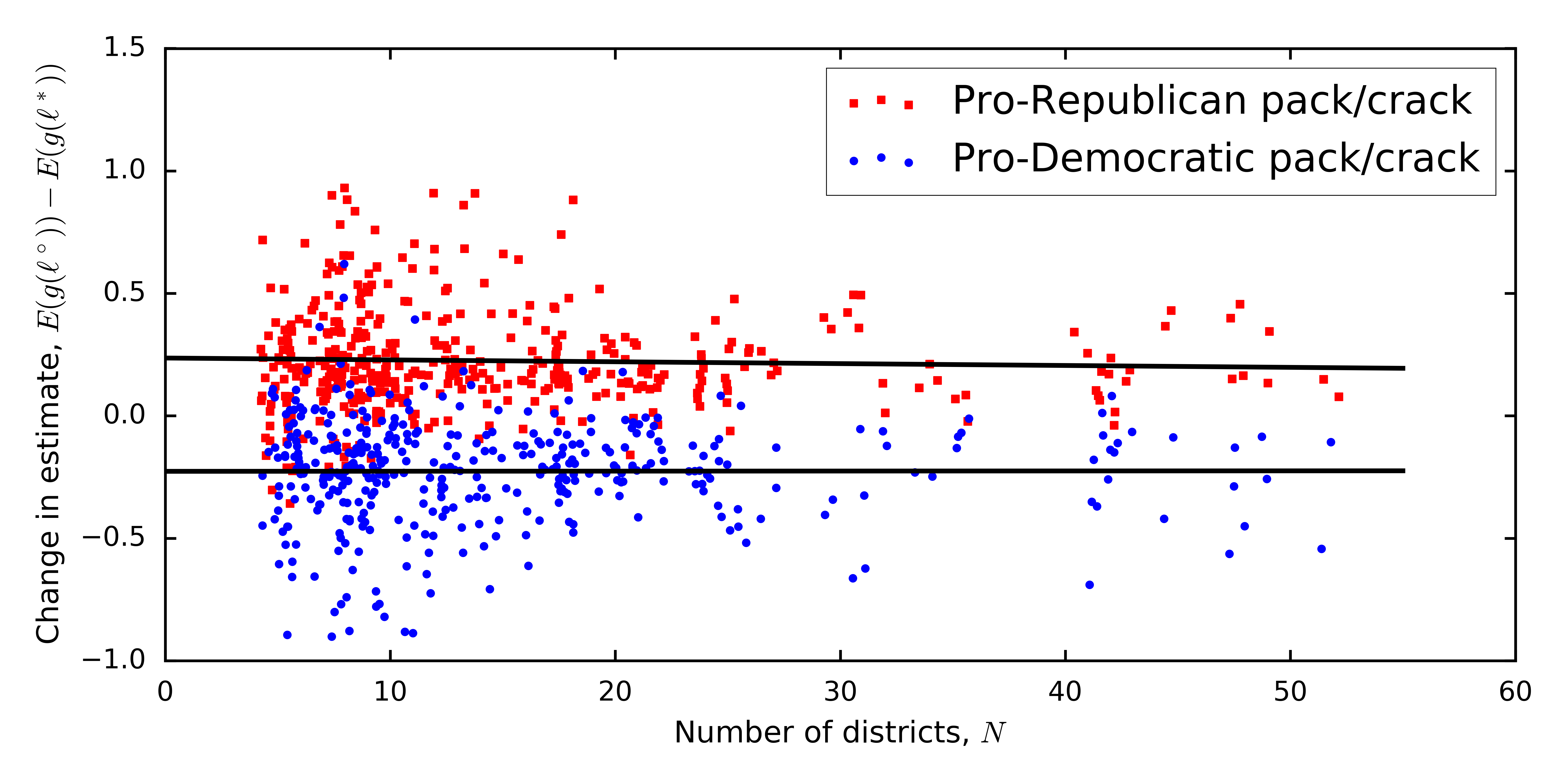
Figure 6 depicts values of the expression in (3) under the flipping of one seat via SPC. This figure is analogous to Figure 4, which shows the corresponding results for the $S$-declination. If this model faithfully recorded the effects of gerrymandering — and hence packing and cracking — we would see the red squares vertically clustered around $+1$ and the blue circles vertically clustered around $-1$. However, as seen in Figure 6, this is not at all the case.

4.2.2 Qualitative explanation for why Chen-Cottrell model fails.

Figure 7: (A) Example showing how cracking a district could lead to essentially no change in the expected number of democratic districts, as determined by the logistic model. (B) Example showing how packing a district could lead to a moderate decrease in the expected number of democratic districts, as determined by the logistic model.

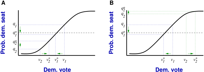
We believe there is a simple reason for the relative invisibility of packing and cracking to the logistic model. When districts are redrawn so that, say a 55% democratic district becomes 45% democratic, the map drawers are doing so with a detailed understanding of the partisan composition of each affected district. While the gerrymander will degrade over time and may be susceptible to wave elections, the probability of the particular district electing a democratic legislator goes from essentially one to essentially zero. However, the probability of that district being democratic as determined by the fitted logistic curve will change by a much smaller amount. Furthermore, the decrease in probability for the given district will be at least partially offset by increased probabilities in the districts to which the democratic voters are now allocated.

Figure 7 illustrates how cracking or packing a single district could lead to at most a small change in the expected number of seats as determined by a sum over the probabilities obtained from the logistic regression. Since we are setting $p_{i}=0+1\cdot\ell_{i}=\ell_{i}$, there is only a single vote fraction associate to each district, which we denote by $v_{i}$. We write $q_{i}$ for $F(\beta_{0}+\beta_{1}v_{i})$, the probability of a democratic win in district $i$. The corresponding values after SPC are denoted by $v^{*}_{i}$ and $q^{*}_{i}$, respectively. Suppose District $1$ is being flipped from republican to democratic and suppose District $2$ received some of the reallocated democratic votes. In Figure 7.A, we see that the reduction in probability from $q_{1}$ to $q^{*}_{1}$ is almost exactly offset by a corresponding increase from $q_{2}$ to $q^{*}_{2}$. In Figure 7.B, there is almost no change from $q_{2}$ to $q^{*}_{2}$, leading to a net decrease in the expected number of democratic seats. However, the net decrease is still much less than one.

4.2.3 Choosing $\gamma_{0[j]}$ and $\gamma_{1[j]}$ through linear regression.

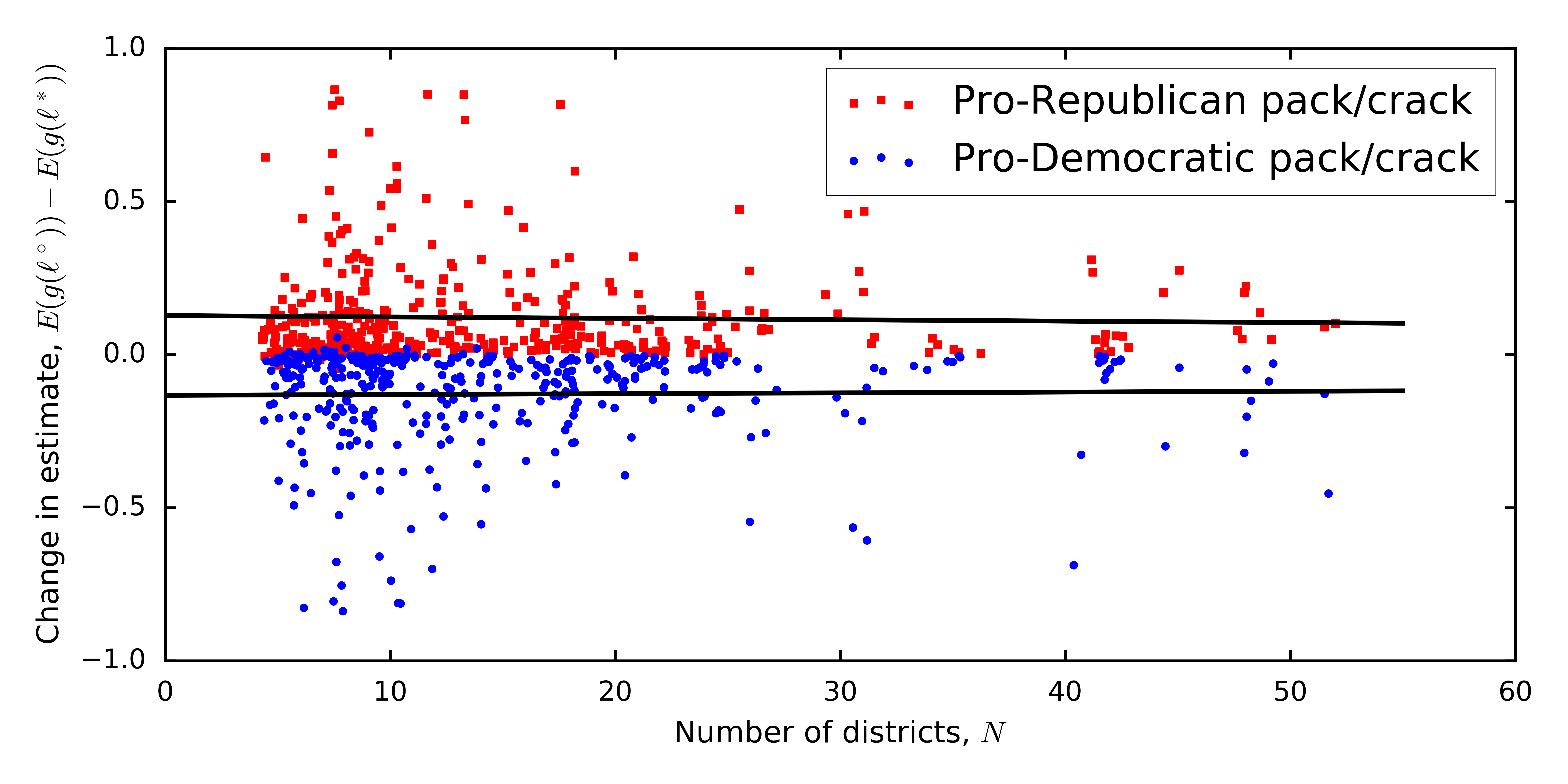
The choice of $(\gamma_{0[j]},\gamma_{1[j]})=(0,1)$ for all $j$ is useful for understanding the structural reasons for why the presidential-vote logistic model does not record partisan gerrymandering. However, an ordinary linear regression fitted to the presidential and legislative votes should yield a quantitatively superior model. If we perform an ordinary linear regression using a random effects model, we obtain the estimates of the coefficients $\gamma_{0[j]}$ and $\gamma_{1[j]}$ displayed in Table 2. But these more defensible choices of $\gamma_{0[j]}$ and $\gamma_{1[j]}$ do little to improve the correspondence between SPC and the difference $E(g(\boldsymbol{\ell}^{\circ}))-E(g(\boldsymbol{\ell}^{*}))$. In Figure 8 we display the values of

$$E(g(\boldsymbol{\ell}^{\circ}))-E(g(\boldsymbol{\ell}^{*}))=\\ \sum_{i=1}^{N}F(\beta_{0[j]}+\beta_{1[j]}(\gamma_{0[j]}+\gamma_{1[j]}\ell^{\circ}_{i}))-\sum_{i=1}^{N}F(\beta_{0[j]}+\beta_{1[j]}(\gamma_{0[j]}+\gamma_{1[j]}\ell^{*}_{i}))$$ (4)

as $j$ indexes the years from 1972 to 2012. While there is better separation between the two populations, the absolute change in the expected number of seats is only about a tenth of a seat, even worse than when we conflated legislative and presidential votes.

Table 2: Random effect estimates from linear and logistic models. The second and third columns contain estimates of the coefficients $\gamma_{0[j]}$ and $\gamma_{1[j]}$ for linear regression of presidential vote regressed on legislative vote for presidential election years using a random effects model where intercept and slope were random effects. The fourth and fifth columns list estimates for the intercepts and slopes for the random effects logistic regression of district outcome on presidential vote for presidential election years.

Year ($j$)	Intercept ($\gamma_{0[j]}$)	Slope ($\gamma_{1[j]}$)	Intercept ($\beta_{0[j]}$)	Slope ($\beta_{1[j]}$)
1972	0.197	0.362	-3.55	9.6
1976	0.292	0.391	-7.91	17.3
1980	0.234	0.427	-5.49	12.7
1984	0.183	0.451	-6.19	16.0
1988	0.255	0.395	-5.58	13.1
1992	0.250	0.527	-7.71	15.8
1996	0.234	0.625	-11.37	20.8
2000	0.210	0.592	-8.22	16.3
2004	0.176	0.622	-10.63	21.7
2008	0.157	0.691	-9.38	18.9
2012	0.082	0.850	-19.18	37.2

Figure 8: Plot of data in Figure 6 using using (4) instead of (3). The linear regression lines are $0.128-0.000N$ ($r^{2}<0.01$, $\mathrm{RMSE}=0.159$) and $-0.133+0.000N$ ($r^{2}<0.01$, $\mathrm{RMSE}=0.163$), respectively.

4.2.4 Noise in the linear model.

One possibility worth examining is that the failure of the Chen-Cottrell model in our simulations of SPC is due to our modeling of the relationship between presidential vote and legislative vote as linear. The linear relationship is much truer in some years than others and, with the exception of 2012, is never completely convincing. But arguing against this possibility is the fact that data points from 2012 are included in Figures 6 and 8 and there is no subpopulation clustered around $\pm 1$. In fact, the sensitivity does seem better for 2012 with a median (absolute-value) change of just over one half. Regardless, any “noise” added to the relationship will merely impede the ability of the presidential-vote logistic regression model to record packing and cracking.

Figure 9: Plot of democratic presidential vote fraction versus legislative seat winner (points have been jittered) for the year 2008. The fitted logistic curve with parameters $\beta_{0}=-9.38$ and $\beta_{1}=18.9$ (from Table 2) is also shown.

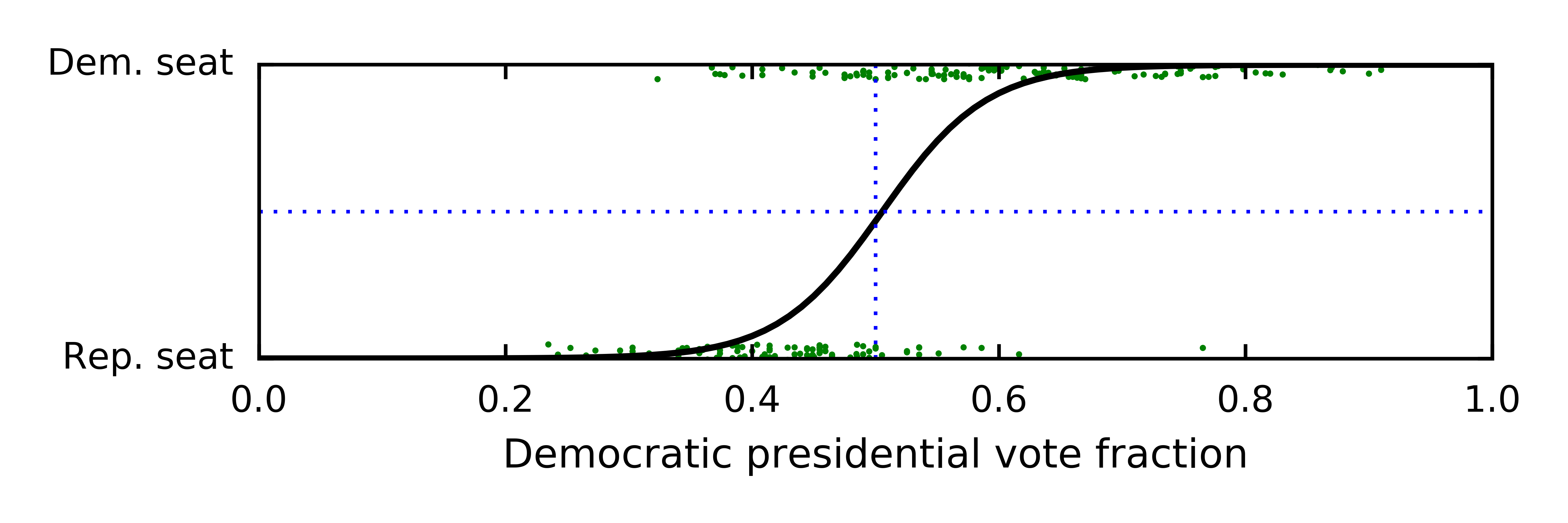
A model that postulates a linear relation between the proportion of legislative and presidential vote in a district induces a probability model for the probability of a democratic win in a district given the presidential vote. It can be shown that the effect of presidential vote in the probability model decreases to zero as the correlation between legislative and presidential vote decreases to zero. In other words, if there is a significant amount of noise in the relation between legislative and presidential vote, presidential vote will be a weak predictor of the winner of a district, further degrading the ability of the logistic model to capture the effects of gerrymandering.

Remark 4.

Incumbent US House Representatives typically win upwards of 90% of their races. In particular, the fitted logistic regression curves will be very different for the classes of 1) democratic incumbents, 2) republican incumbents and 3) no incumbents. There is no reason incumbency cannot be incorporated into the Chen-Cottrell model, but there is one very important issue: The assumptions made for the distribution of incumbents will have a significant impact on the conclusions. Any historical gerrymander will change the relative proportion of incumbents which, in turn, will affect the future probabilities for who wins which seats.

5 Conclusion

If the net impact of partisan gerrymandering on the US democracy is understood to be minimal on a national level, there are likely to be only piecemeal efforts to mitigate its influence. If, on the other hand, its effect is shown to be large, there is likely to be a greater political and judicial will to take steps to counter it on a national level. Unfortunately, as detailed in [CC16], there are manifest difficulties in directly measuring the net effect of gerrymandering. The Chen-Cottrell approach inarguably addresses some of these difficulties. For example, by using contemporaneous electoral data, it can remove year-to-year effects. And, assuming the simulations draw from the space of all districts in an appropriate manner, it can account for geographic clustering. (Unfortunately, there is no objectively “correct” distribution to draw from. Even showing that the draws are sufficiently random is a difficult matter.)

However, as we have attempted to show above, performing a logistic regression on presidential data is fatally flawed for this particular purpose. Not only do our simulations indicate that it does not effectively record packing and cracking, but we believe there are convincing theoretical reasons for concluding it does not. The $S$-declination, defined and studied in this paper, provides a measure of the number of seats gained/lost through partisan gerrymandering. The validity of the $S$-declination for this purpose is strongly supported by simulated packing and cracking (Figure 4).

Neither we nor Royden and Li take into account geographic clustering that has been shown to exist in [CR13]. Nonetheless, their results and our Table 1 suggest that the net number of seats won by gerrymandering is likely to be significant. And, as noted in [War17], it is not clear to what degree district plans should be allowed to exacerbate (or mitigate) inherent geographic distributions. Regardless, if there is only a minimal net effect of gerrymandering on a national level, we find no evidence in [CC16] to support this position.

6 Acknowledgments

The US congressional data through 2014 was provided by [Jac17]. The election data was analyzed using the python-based SageMath [S⁺16]. See [War17] for packages used for, and details of, the imputation of votes. Additional Python packages employed in this paper were Matplotlib [Hun07] for plotting and visualization and SciPy [JOP⁺] for statistical methods. Estimated coefficients for the linear and logistic regressions were computed using the lme4 package [BMBW15] in R [R C13]. We thank Jordan Ellenberg for suggesting a second SPC algorithm to check.

References

- [AAG06] Alan I. Abramowitz, Brad Alexander, and Matthew Gunning. Incumbency, redistricting, and the decline of competition in U.S. House elections. Journal of Politics, 68(1):75–88, 2006.
- [BMBW15] Douglas Bates, Martin Mächler, Ben Bolker, and Steve Walker. Fitting linear mixed-effects models using lme4. Journal of Statistical Software, 67(1):1–48, 2015.
- [CC16] Jowei Chen and David Cottrell. Evaluating partisan gains from congressional gerrymandering: Using computer simulations to estimate the effect of gerrymandering in the U.S. House. Elec. Stud., 44:329–340, 2016.
- [CR13] Jowei Chen and Jonathan Rodden. Unintentional gerrymandering: Political geography and electoral bias in legislatures. Quart. J. of Pol. Sci., 8:239–269, 2013.
- [Gan16] Patrick Gannon. Political gerrymandering nears ‘too far’. Elizabeth City Daily Advance, June 20, 2016. accessed online, July 12, 2017. Syndicated column.
- [Hun07] J. D. Hunter. Matplotlib: A 2D graphics environment. Computing In Science & Engineering, 9(3):90–95, 2007.
- [Jac17] Gary C. Jacobson. Private communication, 2017.
- [JOP+ ] Eric Jones, Travis Oliphant, Pearu Peterson, et al. SciPy: Open source scientific tools for Python, 2001–. [Online; accessed 2017-02-08].
- [KMM+16] Jonathan S. Krasno, Daniel Magleby, Michael D. McDonald, Shawn Donahue, and Robin E Best. Can gerrymanders be measured? an examination of Wisconsin’s state assembly. May 22, 2016. Available at SSRN: https://ssrn.com/abstract=2783144.
- [MB15] Michael D. McDonald and Robin E. Best. Unfair partisan gerrymanders in politics and law: A diagnostic applied to six cases. Elect. Law J., 14(4):312–330, Dec 2015.
- [McG14] Eric McGhee. Measuring partisan bias in single-member district electoral systems. Legis. Stud. Q., 39:55–85, 2014.
- [MS92] J. F. Monahan and L. A. Stefanski. Normal scale mixture approximations to and computation of the logistic-normal integral. In N. Balakrishnan, editor, Handbook of the Logistic Distribution, volume 123 of Statistics, textbooks and monographs, pages 529–540. Marcel Dekker, New York, 1992.
- [MS15] Eric McGhee and Nicholas Stephanopoulos. Partisan gerrymandering and the efficiency gap. 82 University of Chicago Law Review, 831, 2015. 70 pages. U of Chicago, Public Law working Paper No. 493. Available at SSRN: https://ssrn.com/abstract=2457468.
- [MSK15] Anthony J. McGann, Charles Anthony Smith, and Michael Latner J. Alex Keena. A discernable and manageable standard for partisan gerrymandering. Elect. Law J., 14(4):295–311, Dec 2015.
- [NGCH90] Richard G. Niemi, Bernard Grofman, Carl Carlucci, and Thomas Hofeller. Measuring compactness and the role of a compactness standard in a test for partisan and racial gerrymandering. J. of Pol., 52:1155–1181, Nov. 1990.
- [R C13] R Core Team. R: A Language and Environment for Statistical Computing. R Foundation for Statistical Computing, Vienna, Austria, 2013. ISBN 3-900051-07-0.
- [RL17] Laura Royden and Michael Li. Extreme maps. Technical report, Brennan Center for Justice, 2017.
- [S+16] W. A. Stein et al. Sage Mathematics Software (Version 7.1). The Sage Development Team, 2016. http://www.sagemath.org.
- [Wan16] Samuel S.-H. Wang. Three tests for practical evaluation of partisan gerrymandering. Stanford Law Review, 68:1263–1321, June 2016.
- [War17] Gregory S. Warrington. Quantifying gerrymandering using the vote distribution. ArXiv e-prints, arXiv:1705.09393, May 2017.