Laser beam imaging from the speckle pattern of the off-axis scattered intensity

Abstract

We study the inverse problem of localization (imaging) of a laser beam from measurements of the intensity of light scattered off-axis by a Poisson cloud of small particles. Starting from the wave equation, we analyze the microscopic coherence of the scattered intensity and show that it is possible to determine the laser beam from the speckle pattern captured by a group of CCD cameras. Two groups of cameras are sufficient when the particles are either small or large with respect to the wavelength. For general particle sizes the accuracy of the laser localization with two groups of cameras is subject to knowing the scattering properties of the cloud. However, three or more groups of cameras allow accurate localization that is robust to uncertainty of the type, size, shape and concentration of the particles in the cloud. We introduce a novel laser beam localization algorithm and give some numerical illustrations in a regime relevant to the application of imaging high energy lasers in a maritime atmosphere.

1 Introduction

We study an inverse problem for the wave equation, motivated by the application of detection and characterization of high energy laser beams propagating in a maritime atmosphere. The data are gathered by sensors that do not lie in the footprint of the beam, but at remote locations off its axis. These sensors measure the intensity of incoherent light scattered by a cloud of particles suspended in air (aerosols), with sizes ranging from a few nanometers to a hundred micrometers [12]. Maritime environments have a mixture of aerosols like sea salts, dust particles, water droplets, etc., with concentration and composition of the cloud depending on factors such as weather and location [11, 18]. The aerosols are typically modeled as spherical particles, so that their interaction with the laser beam can be described by the Mie scattering theory [9, 17]. This seems to capture well experimental observations [3, 18, 11].

We refer to [3, 15, 12] for studies of detection of laser beams from off-axis measurements of the scattered intensity. Pulsed laser beam localization is studied in [7, 20], using a camera that can measure the intensity resolved over both time and direction of arrival. We are interested in continuous wave (time harmonic) laser beams, where arrival times cannot be measured. The localization of such lasers was studied in [6] using intensity measurements at two cameras placed in the focal plane of lenses which Fourier transform the light wave in order to resolve the intensity over direction of arrival. The setup requires knowledge of the focal length of the lenses, which depends on the wavelength $\lambda$ of the laser. The localization becomes ambiguous when the two cameras and the axis of the beam are in the same plane, as shown in [6], where an improvement based on the relative radiance of scattering at the cameras is proposed. This approach may be susceptible to uncertainty in the composition of the cloud of particles and of the mathematical model of the scattered intensity.

In this paper we introduce an original method for laser beam localization, using the microscopic coherence properties of the intensity measured off-axis. It has the advantage of robustness to uncertainty of the wavelength of the laser beam, the shape and size of the particles, and the concentration and composition of the cloud. However, it requires more measurements of the intensity, at two or more groups of cameras, and these measurements must be spatially resolved according to the speckle size, which is determined by the dominant type of particles in the cloud. If most particles are small with respect to the wavelength, the speckle size is of the order $\lambda$, and the cameras may need to be equipped with microscopes for proper spatial resolution. The speckle size increases for larger particles, so conventional CCD cameras have sufficient resolution.

We derive from first principles, starting from the wave equation, the mathematical model of the intensity of the incoherent light scattered off-axis by a cloud of particles encountered by the laser beam. The locations of the particles are modeled by a Poisson point process, which corresponds to having statistically independent numbers of particles in non-overlapping domains. We begin with a Poisson cloud of identical, spherical particles of radius $a$, and derive a simple model of the scattered intensity using the single scattering (Born) approximation and the Mie theory. This gives an explicit mathematical expression of the incoherent intensity that shows the dependence of the speckle pattern on the ratio $a/\lambda$. Then we explain how the results generalize to mixtures of particles of different sizes and shapes, and to multiple scattering regimes, as long as the waves reaching the cameras do not travel longer than the transport mean free path in the Poisson cloud. This is the characteristic length scale over which the light forgets its initial direction due to multiple scattering [19]. At larger travel distances the angle of arrival of the recorded intensity is not meaningful, and imaging should be based on diffusion models.

In this paper we image at distances smaller than the transport mean free path, and show how to extract information about the laser beam from the speckle pattern of the off-axis scattered intensity. We introduce a novel imaging algorithm and analyze how many measurements are needed for accurate beam localization that is robust to uncertainty of the cloud of particles and therefore of the model of the measurements.

The paper is organized as follows: We begin in section 2 with the formulation of the problem and the scaling regime. Then we give in section 3 the statistics of the waves scattered off-axis, and describe in detail the covariance of the speckle intensity. The imaging algorithm is introduced in section 4 and its performance is illustrated with some numerical simulations in section 5. We end with a summary in section 6.

2 Formulation of the problem

We give here a simple model of the interaction of a laser beam with a Poisson cloud of particles. We derive it in section 2.1, using the single scattering approximation and the Mie scattering theory, in the scaling regime described in section 2.2.

2.1 Model of the scattered waves

Let us begin with the Helmholtz equation

$$\Delta u(\vec{\itbf x})+(k+ik_{\rm d})^{2}\big{[}1+V(\vec{\itbf x})\big{]}u(\vec{\itbf x})=0,$$ (1)

satisfied by a time harmonic wave $u(\vec{\itbf x})e^{-i\omega t}$ at frequency $\omega$ and location $\vec{\itbf x}\in\mathbb{R}^{3}$. The wave propagates in a medium with constant wave speed $c$, containing small particles modeled by the scattering potential $V(\vec{\itbf x})$. The coefficient $k$ in (1) is the wavenumber

$$k=\frac{\omega}{c}=\frac{2\pi}{\lambda},$$

and $k_{\rm d}$ is a small damping parameter, satisfying $k\gg k_{\rm d}>0$, which models attenuation in the medium and extinction of the beam due to scattering by the cloud of particles [18].

The scattering potential $V(\vec{\itbf x})$ is supported on the particles, modeled as spheres $B(a_{j},\vec{\itbf x}_{j})$ of radius $a_{j}$ and center $\vec{\itbf x}_{j}$, for $j\geq 1$,

$$V(\vec{\itbf x})=\sum_{j}\sigma_{j}{\bf 1}_{B(a_{j},\vec{\itbf x}_{j})}(\vec{\itbf x}).$$ (2)

Here ${\bf 1}_{B(a_{j},\vec{\itbf x}_{j})}$ is the indicator function of the support of the $j$-th particle and $\sigma_{j}$ is its reflectivity, the change in the index of refraction. The locations $\{\vec{\itbf x}_{j}\}_{j\geq 1}$ of the particles are modeled as a Poisson point process with homogeneous intensity $\rho$. This is the mean number of particles per unit volume, and it can be written as

$$\rho=1/\ell^{3},$$ (3)

with $\ell$ interpreted as the mean distance between the particles. We consider first identical particles with radius $a$, so that we can study the effect of the ratio $a/\lambda$ on the speckle pattern registered at the cameras. As explained later, the imaging method applies to a mixture of particle sizes and shapes.

The wave field

$$u(\vec{\itbf x})=u_{\rm b}(\vec{\itbf x})+u_{\rm s}(\vec{\itbf x})$$ (4)

is the superposition of the incident field $u_{\rm b}(\vec{\itbf x})$, which models the laser beam, and the scattered field $u_{\rm s}(\vec{\itbf x})$. For convenience in the calculations, we assume that the beam has a Gaussian profile, with axis parametrized by $z$ and beam waist in the plane $z=0$. The radius at the waist is denoted by $r_{o}$. It is large with respect to the wavelength, so we are in a paraxial regime with the beam modeled by [13, Chapter 5]

$$u_{\rm b}(\vec{\itbf x})=\frac{r_{o}^{2}}{R_{z}^{2}}\exp\Big{(}-\frac{|{\itbf x}|^{2}}{R_{z}^{2}}+ikz-k_{\rm d}z\Big{)},\quad\quad R_{z}=r_{o}\Big{(}1+\frac{2iz}{kr_{o}^{2}}\Big{)}^{1/2}.$$ (5)

Here we introduced the system of coordinates $\vec{\itbf x}=({\itbf x},z)$, with $z$ on the axis of the laser beam, and the two-dimensional vector ${\itbf x}$ in the plane orthogonal to it.

In the single scattering (Born) approximation, the scattered field is modeled by the solution of the inhomogeneous Helmholtz equation

$$\Delta u_{\rm s}+(k+ik_{\rm d})^{2}u_{\rm s}=-(k+ik_{\rm d})^{2}V(\vec{\itbf x})u_{\rm b}(\vec{\itbf x}),$$ (6)

satisfying the Sommerfeld radiation condition away from the beam and outside the support of $V(\vec{\itbf x})$. It is given explicitly by

$$u_{\rm s}(\vec{\itbf x})=(k+ik_{\rm d})^{2}\int_{\mathbb{R}^{3}}d\vec{\itbf y}\,G(\vec{\itbf x},\vec{\itbf y})V(\vec{\itbf y})u_{\rm b}(\vec{\itbf y}),$$ (7)

where

$$G(\vec{\itbf x},\vec{\itbf y})=\frac{1}{4\pi|\vec{\itbf x}-\vec{\itbf y}|}\exp\big{[}(ik-k_{\rm d})|\vec{\itbf x}-\vec{\itbf y}|\big{]}$$ (8)

is the Green’s function. Using the model (2) of the scattering potential, we rewrite (7) as a sum over the particles

$$u_{\rm s}(\vec{\itbf x})\approx k^{2}\sum_{j}{\mathfrak{I}}_{\rm Mie}\big{(}\alpha(\vec{\itbf x},\vec{\itbf x}_{j});ka,\sigma\big{)}G(\vec{\itbf x},\vec{\itbf x}_{j})u_{\rm b}(\vec{\itbf x}_{j}).$$ (9)

Here we neglected the small damping term $k_{\rm d}$ in the multiplicative factor $(k+ik_{\rm d})^{2}$, and introduced the Mie scattering kernel ${\mathfrak{I}}_{\rm Mie}$ [17, Chapter 9], which depends on the ratio of the radius $a$ of the particles and the wavelength (i.e., $ka$), the reflectivity $\sigma$ and the angle $\alpha(\vec{\itbf x},\vec{\itbf x}_{j})$ from $\vec{\itbf x}$ to $\vec{\itbf x}_{j}$.

For small (point-like) particles, with radius $a$ satisfying $ka\ll 1$, the scattering is approximately isotropic and we can approximate the kernel ${\mathfrak{I}}_{\rm Mie}$ by a constant

$${\mathfrak{I}}_{\rm Mie}\big{(}\alpha(\vec{\itbf x},\vec{\itbf x}_{j});ka,\sigma\big{)}\approx\sigma\frac{4\pi a^{3}}{3}=:\eta.$$ (10)

When $ka\gtrsim 1$ but $\sigma$ is small enough so that $\sigma ka\ll 1$, the scattering kernel is approximated by the Rayleigh-Gans formula [17, Chapter 7]

$${\mathfrak{I}}_{\rm RG}\big{(}\alpha(\vec{\itbf x},\vec{\itbf x}_{j});ka,\sigma\big{)}=\eta\frac{3\sqrt{2\pi}J_{3/2}\big{[}2ka\alpha(\vec{\itbf x},\vec{\itbf x}_{j})\big{]}}{2\big{[}2ka\alpha(\vec{\itbf x},\vec{\itbf x}_{j})\big{]}^{3/2}},$$ (11)

where $J_{3/2}(t)=\sqrt{2/\pi}(\sin(t)-t\cos(t))/t^{3/2}$ is the Bessel function of the first kind and of order $3/2$. The expression (11) reduces to (10) in the limit $ka\to 0$, and shows that scattering is peaked in the forward direction, at angles $\alpha\sim 1/(ka)$, when $ka\gtrsim 1$. The forward scattering is also predicted by the Mie scattering kernel ${\mathfrak{I}}_{\rm Mie}$, which should be used for larger $\sigma$. This has a complicated expression given in [17, Chapter 9].

2.2 Scaling

Our analysis of the statistics of the scattered field (9) is carried out in a regime defined by the relations

$$\lambda\ll\ell\ll r_{o}\ll L_{\itbf x}\ll L_{z},\qquad\lambda\ll d_{A}\ll r_{o},$$ (12)

between the important length scales in the problem: the wavelength $\lambda$, the particle size $a$, the mean distance $\ell$ between the particles, the radius $r_{o}$ of the laser beam, the diameter $d_{A}$ of the domain (aperture) $A$ of the camera, the typical offset (cross-range) $L_{\itbf x}$ of the camera from the axis of the beam and the typical distance (range) $L_{z}$ of the camera along the axis of the beam, measured from the waist (the laser source).

The scaling relations (12) are motivated by the application of high energy laser imaging in a marine atmosphere, where the wavelength $\lambda$ is of the order of $1\mu{\rm m}$, and the particle radius $a$ may be small or large with respect to $\lambda$. The mean distance $\ell$ between the particles is of the order of $1$mm. It is much larger than the wavelength, so multiple scattering is not too strong and the Born approximation captures approximately the microscopic coherence properties of the speckle pattern. The radius of the beam $r_{o}$ is in the range of $0.1-1$m. The diameter $d_{A}$ of the camera is of the order of hundreds of wavelengths. It is at cross-range $L_{\itbf x}$ of the order of $100$m and at range $L_{z}$ of the order of $1$km.

In this scaling regime, the Rayleigh length $L_{\rm R}$, which is the distance at which the beam doubles its radius due to diffraction, satisfies

$$L_{\rm R}=\frac{kr_{o}^{2}}{2}\gg L_{z}.$$ (13)

Thus, we may neglect diffraction effects and approximate in (5)

$$R_{z}\approx r_{o}~{}~{}\mbox{for}~{}z=O(L_{z}).$$ (14)

Nevertheless, it is possible to extend the results to scalings where $L_{\rm R}\sim L_{z}$ and $R_{z}$ is a smooth $z$-dependent function, as defined in (5).

The damping term $k_{\rm d}$, which models attenuation in the medium, is used in our analysis to ensure the integrability of the terms in the sum (9). We assume henceforth that

$$k_{\rm d}L_{\itbf x}\ll 1,$$ (15)

so we can neglect the attenuation over the cross-range offsets from the laser axis to the cameras. This assumption simplifies the expression of the correlation function of the intensity of the scattered field, derived in the next section. The results extend to $k_{\rm d}L_{\itbf x}\gtrsim 1$, but from the practical point of view the intensity may be too weak to be detected by such remote cameras.

3 Statistics of the scattered waves

We describe here the statistics of the scattered wave field $u_{\rm s}(\vec{\itbf x})$ modeled by equation (9). We begin in section 3.1 with a summary of basic results for Poisson point processes. Then we derive in section 3.2 the expression of the covariance function of the intensity $|u_{\rm s}(\vec{\itbf x})|^{2}$ measured at the camera, for the case of small particles. The case of larger particles is analyzed in section 3.3, and the generalization to mixtures of particles is in section 3.5. We also analyze in section 3.4 the level sets of the covariance function near its peak, and show that they can be approximated by ellipsoids with axes that depend on the axis of the laser beam. This is used in the imaging algorithm described in section 4.

3.1 Basic results on Poisson point processes

Recall from section 2.1 that the locations $\{\vec{\itbf x}_{j}\}_{j\geq 1}$ of the particles are modeled by a Poisson cloud with homogeneous intensity $\rho$. Here we summarize from [10] some basic results on Poisson processes, needed to calculate the statistical moments of the scattered wave field.

By Campbell’s theorem [10, Section 3.2], for any function $f(\vec{\itbf x})$ satisfying the condition $\min(|f|,1)\in L^{1}(\mathbb{R}^{3})$, the characteristic function of the random variable $F=\sum_{j}f(\vec{\itbf x}_{j})$ is given by

$$\mathbb{E}[e^{itF}]=\exp\Big{[}\rho\int_{\mathbb{R}^{3}}d\vec{\itbf x}\,\big{(}e^{itf(\vec{\itbf x})}-1\big{)}\Big{]},$$ (16)

where $\mathbb{E}[\cdot]$ denotes expectation with respect to the Poisson point process distribution. Moreover, if the function $f$ is in $L^{1}(\mathbb{R}^{3})\cap L^{2}(\mathbb{R}^{3})$, then $F=\sum_{j}f(\vec{\itbf x}_{j})$ is an integrable and square-integrable random variable with

$$\mathbb{E}[F]=\rho\int_{\mathbb{R}^{3}}d\vec{\itbf x}\,f(\vec{\itbf x}),\quad\quad\mathbb{E}[F^{2}]=\rho\int_{\mathbb{R}^{3}}d\vec{\itbf x}\,f^{2}(\vec{\itbf x}).$$ (17)

The following lemma allows us to calculate the moments of the scattered wave field:

Lemma 1.

Let $f_{1},\ldots,f_{4}$ be functions in $L^{1}(\mathbb{R}^{3})\cap L^{2}(\mathbb{R}^{3})$, that integrate to zero

$$\int_{\mathbb{R}^{3}}d\vec{\itbf x}\,f_{q}(\vec{\itbf x})=0,\quad q=1,\ldots,4,$$ (18)

and denote $F_{q}=\sum_{j}f_{q}(\vec{\itbf x}_{j})\,$ for $q=1,\ldots,4$. We have

$$\mathbb{E}[F_{1}F_{2}]=\rho\int_{\mathbb{R}^{3}}d\vec{\itbf x}\,f_{1}(\vec{\itbf x})f_{2}(\vec{\itbf x}),$$ (19)

and

$$\mathbb{E}[F_{1}F_{2}F_{3}F_{4}]= \mathbb{E}[F_{1}F_{2}]\mathbb{E}[F_{3}F_{4}]+\mathbb{E}[F_{1}F_{3}]\mathbb{E}[F_{2}F_{4}]+\mathbb{E}[F_{1}F_{4}]\mathbb{E}[F_{2}F_{3}]$$

$$+\rho\int_{\mathbb{R}^{3}}d\vec{\itbf x}\,f_{1}(\vec{\itbf x})f_{2}(\vec{\itbf x})f_{3}(\vec{\itbf x})f_{4}(\vec{\itbf x}).$$ (20)

Proof.

The proof follows from the identity

$$\mathbb{E}\Big{[}\prod_{q=1}^{n}F_{q}\Big{]}=(-i)^{n}\frac{\partial^{n}}{\partial t_{1}\cdots\partial t_{n}}\mathbb{E}\Big{[}\prod_{q=1}^{n}e^{it_{q}\sum_{j}f_{q}(\vec{\itbf x}_{j})}\Big{]}\Big{|}_{t_{1},\ldots,t_{n}=0}$$ (21)

and [10, Corollary 3.1], which states that

$$\mathbb{E}\Big{[}\prod_{q=1}^{n}e^{it_{q}\sum_{j}f_{q}(\vec{\itbf x}_{j})}\Big{]}=\exp\Big{[}\rho\int_{\mathbb{R}^{3}}d\vec{\itbf x}\,\big{(}e^{i\sum_{q=1}^{n}t_{q}f_{q}(\vec{\itbf x})}-1\big{)}\Big{]}.$$ (22)

Equation (19) is obtained by substituting (22) in (21), setting $n=2$, and using (18). Similarly, equation (20) follows by substituting (22) in (21) and setting $n=4$. ∎

When the functions $f_{q}$ are bounded and compactly supported, as is the case in the model (9), we note that the last term in (20) is negligible with respect to the others if the volume of support of the functions is large compared to $1/\rho=\ell^{3}$. This condition holds in our scaling regime, and the implication is that the fourth-order moments satisfy the Gaussian summation rule, for zero-mean Gaussian processes. We use this observation in the next sections and in appendix B, to calculate the correlation of the intensity of the scattered field.

3.2 Statistics of the scattered field for small scatterers

If the particles are small, with radius $a\ll\lambda$, the scattering kernel in (9) is approximated by the constant $\eta$ defined in (10). The next proposition, proved in appendix A, gives the mathematical expression of the mean and covariance function of the scattered field:

Proposition 2.

In the scaling regime defined in section 2.2, the mean scattered field at point $\vec{\itbf x}$ in the aperture of the camera is approximately zero,

$$\mathbb{E}\big{[}u_{\rm s}(\vec{\itbf x})\big{]}\approx 0.$$ (23)

Moreover, the covariance function of the scattered field evaluated at points $\vec{\itbf x}_{1}=\vec{\itbf X}+\vec{\itbf x}/2$ and $\vec{\itbf x}_{2}=\vec{\itbf X}-\vec{\itbf x}/2$ in the aperture of the camera is approximated by

$$\mathbb{E}\big{[}u_{\rm s}(\vec{\itbf x}_{1})\overline{u_{\rm s}}(\vec{\itbf x}_{2})\big{]}\approx\frac{\eta^{2}k^{4}\rho r_{o}^{2}e^{-2k_{\rm d}Z}}{32|{\itbf X}|}\Psi\Big{(}k\hat{{\itbf X}}\cdot{\itbf x},\frac{kr_{o}}{2|{\itbf X}|}\hat{{\itbf X}}^{\perp}\cdot{\itbf x},kz\Big{)},$$ (24)

where $\overline{u_{\rm s}}$ denotes the complex conjugate of $u_{\rm s}$ and

$$\Psi(\chi,\xi,\zeta)=\frac{1}{\pi}\int_{0}^{\pi}\exp\Big{[}i\big{(}\sin\alpha\chi+\cos\alpha\zeta\big{)}\Big{]}\exp\Big{(}-\frac{\xi^{2}}{2}\sin^{2}\alpha\Big{)}d\alpha.$$ (25)

Here we decomposed the vectors $\vec{\itbf X}=({\itbf X},{Z})$ and $\vec{\itbf x}=({\itbf x},z)$ in the range coordinates $Z$ and $z$ along the axis of the laser beam, and the two-dimensional vectors ${\itbf X}$ and ${\itbf x}$ in the cross-range plane, which is orthogonal to the beam. All coordinates are with respect to the origin that lies on the axis of the beam, at the waist. We also introduced the unit vector $\hat{{\itbf X}}={\itbf X}/|{\itbf X}|$ and the unit vector $\hat{{\itbf X}}^{\perp}$, which is orthogonal to $\hat{\itbf X}$, and is defined by the rotation of $\hat{\itbf X}$ by ninety degrees in the cross-range plane, counterclockwise.

There are two observations drawn from this proposition: The first is that the scattered field at the camera is incoherent, because its mean (23) is very small with respect to its standard deviation that is approximately equal to the square root of the mean intensity

$$\mathbb{E}\big{[}|u_{\rm s}(\vec{\itbf X})|^{2}]=\frac{\eta^{2}k^{4}\rho r_{o}^{2}e^{-2k_{\rm d}Z}}{32|{\itbf X}|}.$$ (26)

The second observation is that the second moment (24), which approximates the covariance of $u_{\rm s}$, has an anisotropic decay that depends on the orientation of the axis of the laser beam. To estimate the decay of (24) away from the peak, which occurs at $\vec{\itbf x}_{1}=\vec{\itbf x}_{2}$, we consider offsets $\vec{\itbf x}=\vec{\itbf x}_{1}-\vec{\itbf x}_{2}$ aligned with either one of the unit vectors $(\hat{\itbf X},0)$ and $(\hat{\itbf X}^{\perp},0)$ in the cross-range plane, or with the range axis. We have three cases:

1. If $\vec{\itbf x}=|{\itbf x}|(\hat{\itbf X},0)$, the covariance decays like

   $$\Psi(k|{\itbf x}|,0,0)=J_{0}(k|{\itbf x}|)+iH_{0}(k|{\itbf x}|),$$

   where $J_{0}$ is the Bessel function of the first kind and of order zero, and $H_{0}$ is the Struve function of order zero [1, Chapter 12].

2. If $\vec{\itbf x}=|{\itbf x}|(\hat{\itbf X}^{\perp},0)$, the covariance decays like

   $$\Psi\Big{(}0,\frac{kr_{o}|{\itbf x}|}{2|{\itbf X}|},0\Big{)}=I_{0}\left[\frac{1}{4}\Big{(}\frac{kr_{o}|{\itbf x}|}{2|{\itbf X}|}\Big{)}^{2}\right]\exp\left[-\frac{1}{4}\Big{(}\frac{kr_{o}|{\itbf x}|}{2|{\itbf X}|}\Big{)}^{2}\right]$$

   where $I_{0}$ is the modified Bessel function of the first kind and of order zero [1, Chapter 12].

3. If $\vec{\itbf x}=z(0,0,1)$, the covariance decays like

   $$\Psi(0,0,kz)=J_{0}(kz).$$

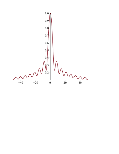
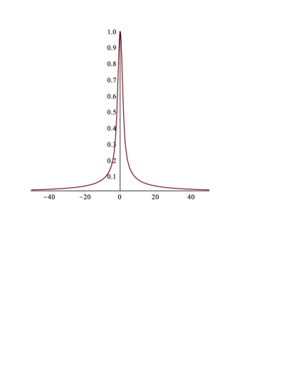
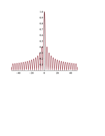
We plot in Figure 1 the functions $|J_{0}(t)+iH_{0}(t)|$, $I_{0}(t^{2}/4)e^{-t^{2}/4}$ and $|J_{0}(t)|\,$ and note that they are large when the argument $t$ is order one. Thus, we estimate that the covariance decays on a scale comparable to the wavelength along the cross-range direction $(\hat{\itbf X},0)$ and the range direction $(0,0,1)$. The decay in range is faster because as shown in Figure 1, the support of the main peak of $|J_{0}(t)|$ is smaller than that of $|J_{0}(t)+iH_{0}(t)|$ by a factor of approximately $2\pi$. The decay of the covariance in the other cross-range direction $(\hat{\itbf X}^{\perp},0)$ is much slower, on the scale $|{\itbf X}|\lambda/r_{o}\gg\lambda$.

Fig. 1: From left to right we display functions $|J_{0}(t)+iH_{0}(t)|$, $I_{0}(t^{2}/4)e^{-t^{2}/4}$ and $|J_{0}(t)|\,$, for $|t|\leq 50$.

The covariance function (24) cannot be calculated directly, because the camera does not measure the wave field $u_{\rm s}(\vec{\itbf x})$, but its intensity $|u_{\rm s}(\vec{\itbf x})|^{2}$. The following proposition, proved in appendix B, shows that the covariance of the measured intensity is approximately the square of the modulus of (24).

Proposition 3.

In the scaling regime described in section 2.2, and for two points $\vec{\itbf x}_{1}=\vec{\itbf X}+\vec{\itbf x}/2$ and $\vec{\itbf x}_{2}=\vec{\itbf X}-\vec{\itbf x}/2$ in the aperture of the camera, we have

$${\rm Cov}\big{(}|u_{\rm s}(\vec{\itbf x}_{1})|^{2},|{u_{\rm s}}(\vec{\itbf x}_{2})|^{2}\big{)}\approx\big{|}\mathbb{E}\big{[}u_{\rm s}(\vec{\itbf x}_{1})\overline{u_{\rm s}}(\vec{\itbf x}_{2})\big{]}\big{|}^{2}.$$ (27)

The covariance of the intensity can be estimated from the speckle pattern captured by the camera, as explained in section 4.1, and Propositions 2 and 3 give that we can use it to extract information about the laser beam. The size of the speckles is related to the scales of decay of the covariance, called correlation lengths. The discussion after Proposition 2 shows that the correlation lengths $l_{{}_{\itbf X}}$ and $l_{{}_{Z}}$ in the directions of the unit vectors $(\hat{\itbf X},0)$ and $(0,0,1)$, which span the plane containing $\vec{{\itbf X}}$ and the axis of the laser beam, are

$$l_{{}_{{\itbf X}}}\sim\lambda,\quad l_{{}_{Z}}\sim\lambda,~{}~{}\mbox{such that}~{}~{}l_{{}_{{\itbf X}}}>l_{{}_{Z}}.$$ (28)

The correlation length in the direction $(\hat{\itbf X}^{\perp},0)$ orthogonal to this plane is much larger

$$l_{{}_{{\itbf X}}}^{\perp}\sim\frac{\lambda|{\itbf X}|}{r_{o}}\gg\lambda.$$ (29)

The distance $|{\itbf X}|$ from the camera to the axis of the laser enters the expression (24) of the covariance in the amplitude factor and the correlation length $l_{{}_{{\itbf X}}}^{\perp}$. In practice, the estimation should not be based on the amplitude, which depends on the model and also on unknown parameters like $\eta$, $\rho$ and $k_{\rm d}Z$. Moreover, $l_{{}_{{\itbf X}}}^{\perp}$ is difficult to estimate from the speckle pattern captured at a small camera with diameter $d_{A}\lesssim l_{{}_{{\itbf X}}}^{\perp}$. Thus, we do not estimate $|{\itbf X}|$ directly from the covariance function (27).

3.3 Statistics of the scattered field for large scatterers

The results stated in the previous section extend readily to the case of larger particles of spherical shape. The only difference in the calculations, which are as in appendices A and B, is that the scattering kernel is no longer the constant $\eta$, but a function rewritten here in the normalized form

$${\mathfrak{I}}_{\rm Mie}(\alpha;ka,\sigma)=\eta{\mathcal{I}}_{\rm Mie}(\alpha;ka,\sigma).$$ (30)

Proposition 4.

In the scaling regime defined in section 2.2, the mean scattered field at the camera is approximately zero. Moreover, the covariance of the intensity at points $\vec{\itbf x}_{1}=\vec{\itbf X}+\vec{\itbf x}/2$ and $\vec{\itbf x}_{2}=\vec{\itbf X}-\vec{\itbf x}/2$ in the aperture of the camera is given by the square of the modulus of the covariance of the scattered field, as in (27). This covariance has the mathematical expression

$$\mathbb{E}\big{[}u_{\rm s}(\vec{\itbf x}_{1})\overline{u_{\rm s}}(\vec{\itbf x}_{2})\big{]} \approx\frac{\eta^{2}k^{4}\rho r_{o}^{2}e^{-2k_{\rm d}Z}}{32\pi|{\itbf X}|}\Psi_{\rm Mie}\Big{(}k\hat{{\itbf X}}\cdot{\itbf x},\frac{kr_{o}}{2|{\itbf X}|}\hat{{\itbf X}}^{\perp}\cdot{\itbf x},kz;ka,\sigma\Big{)},$$ (31)

where

$$\Psi_{\rm Mie}(\chi,\xi,\zeta;ka,\sigma) =\int_{0}^{\pi}d\alpha\,\big{|}{\cal I}_{\rm Mie}\big{(}\alpha;ka,\sigma\big{)}\big{|}^{2}\exp\Big{(}i\big{(}\sin\alpha\chi+\cos\alpha\zeta\big{)}-\frac{\sin^{2}\alpha}{2}\xi^{2}\Big{)}.$$ (32)

The difference between the covariance functions (24) and (31) is the support of the kernel in the scattering angle $\alpha$. While in the case of small particles the kernel is constant, so that all angles $\alpha\in(0,\pi)$ contribute to the integration in (25), for larger particles only smaller angles $\alpha$ contribute in (32) i.e., scattering is in the forward direction.

To illustrate the effect of forward scattering on the covariance (31), suppose that the particles are large such that $ka\gg 1$. Then, the angular opening $\Theta$ of the forward scattering cone is small and we can simplify equations (31-32) by changing the variable of integration $\alpha\to\alpha\Theta$ and using the small argument expansions of the exponent. We obtain

$$\Big{|}\mathbb{E}\big{[}u_{\rm s}(\vec{\itbf x}_{1})\overline{u_{\rm s}}(\vec{\itbf x}_{2})\big{]}\Big{|} \approx\frac{\eta^{2}k^{4}\rho r_{o}^{2}e^{-2k_{\rm d}Z}\Theta}{32\pi|{\itbf X}|}\Big{|}\Psi_{\Theta}\Big{(}k\Theta\hat{{\itbf X}}\cdot{\itbf x},\frac{kr_{o}\Theta^{2}}{2|{\itbf X}|}\hat{{\itbf X}}^{\perp}\cdot{\itbf x},k\Theta^{2}z\Big{)}\Big{|},$$ (33)

where the function

$$\Psi_{\Theta}(\chi,\xi,\zeta) =\int_{0}^{\pi}d\alpha\,\big{|}{\cal I}_{\rm Mie}\big{(}\alpha\Theta;ka,\sigma\big{)}\big{|}^{2}\exp\Big{(}i\big{(}\alpha\chi-\frac{\alpha^{2}}{2}\zeta\big{)}-\frac{\alpha^{2}}{2}\xi^{2}\Big{)}$$ (34)

peaks at the origin and has support of order one in all arguments. To be more explicit, consider the Rayleigh-Gans regime, where $\sigma$ is so small that $\sigma ka\ll 1$. Then, the kernel in (34) simplifies to

$${\cal I}_{\rm Mie}\big{(}\alpha\Theta;ka,\sigma\big{)}\approx\frac{3\sqrt{2\pi}J_{3/2}(2ka\alpha)}{2(2ka\alpha)^{3/2}},$$

and the angular opening of the cone is $\Theta\sim{1}/{(ka)}.$ With this estimate we conclude from (33) that the correlation lengths are

$$l_{{}_{{\itbf X}}}\sim\frac{1}{k\Theta}\sim a,\qquad l_{{}_{{\itbf X}}}^{\perp}\sim\frac{|{\itbf X}|}{kr_{o}\Theta^{2}}\sim\frac{ka^{2}|{\itbf X}|}{r_{o}},\qquad l_{{}_{Z}}\sim\frac{1}{k\Theta^{2}}\sim ka^{2}.$$ (35)

Like in the case of small particles, the largest correlation length is $l_{{}_{{\itbf X}}}^{\perp}$. All correlation lengths are much larger than those defined in (28)–(29), by the factor $ka\gg 1$ in the direction $(\hat{\itbf X},0)$ and the even larger factor $(ka)^{2}$ in the other directions. Furthermore, the decay in the plane defined by the axis of the laser and the vector $\vec{\itbf X}$ is more anisotropic, with $l_{{}_{Z}}\gg l_{{}_{\itbf X}}$.

3.4 The level sets of the correlation function

Propositions 2–4 describe the dependence of the covariance function of the intensity on the unknown axis of the laser beam. The amplitude of the covariance function is model-dependent, so we do not wish to base the imaging on it. We use instead the level sets of the covariance function near its peak, which have a generic dependence on the axis of the laser beam, as we now explain.

Let us define the correlation function of the intensity at points $\vec{\itbf X}\pm\vec{\itbf x}/2$,

$${\rm Corr}\big{(}|u_{\rm s}(\vec{\itbf X}+\vec{\itbf x}/2)|^{2},|{u_{\rm s}}(\vec{\itbf X}-\vec{\itbf x}/2)|^{2}\big{)}=\frac{{\rm Cov}\big{(}|u_{\rm s}(\vec{\itbf X}+\vec{\itbf x}/2)|^{2},|{u_{\rm s}}(\vec{\itbf X}-\vec{\itbf x}/2)|^{2}\big{)}}{\mathbb{E}\big{[}|u_{s}(\vec{{\itbf X}}+\vec{\itbf x}/2)|^{2}\big{]}\mathbb{E}\big{[}|u_{s}(\vec{{\itbf X}}-\vec{\itbf x}/2)|^{2}\big{]}},$$

and use the same decomposition $\vec{\itbf X}=({\itbf X},Z)$ and $\vec{\itbf x}=({\itbf x},z)$ of the mid-point and offset vectors as in Proposition 2. The correlation function attains its maximum value $1$ when the two points coincide, and we study its level sets for small offset vectors $\vec{\itbf x}$, decomposed as

$$\vec{\itbf x}=x(\hat{\itbf X},0)+x^{\perp}(\hat{\itbf X}^{\perp},0)+z(0,0,1),$$ (36)

in the orthonormal basis $\{(\hat{\itbf X},0),(\hat{\itbf X}^{\perp},0),(0,0,1)\}$, with two-dimensional unit vectors $\hat{\itbf X}$ and $\hat{\itbf X}^{\perp}$ defined in Proposition 2. If we scale the components of $\vec{\itbf x}$ by the characteristic correlation lengths,

$$x=\frac{1}{k}\chi,\quad x^{\perp}=\frac{2|{\itbf X}|}{kr_{o}}\xi,\quad z=\frac{1}{k}\zeta,$$ (37)

we conclude from Propositions 2–4 that

$${\rm Corr}\big{(}|u_{\rm s}(\vec{\itbf X}+\vec{\itbf x}/2)|^{2},|{u_{\rm s}}(\vec{\itbf X}-\vec{\itbf x}/2)|^{2}\big{)}\approx \Big{|}\int_{0}^{\pi}d\alpha\,\mathfrak{S}(\alpha)\exp\Big{[}i\big{(}\sin\alpha\chi+\cos\alpha\zeta\big{)}\Big{]}$$

$$\times\exp\Big{(}-\frac{\sin^{2}\alpha}{2}\xi^{2}\Big{)}\Big{|}^{2},$$ (38)

where $\mathfrak{S}(\alpha)$ denotes the scattering kernel, normalized so that $\int_{0}^{\pi}d\alpha\,\mathfrak{S}(\alpha)=1.$ This kernel is non-negative and proportional to $|\mathcal{I}_{\rm Mie}|^{2}$.

Consider a level set ${S}_{\mathfrak{L}}$ of the correlation function at value $1-{\mathfrak{L}}$, for $0<{\mathfrak{L}}\ll 1$. We can approximate it by expanding (38) about $(\chi,\xi,\zeta)=(0,0,0)$, and obtain

$$1-\mathfrak{L} ={\rm Corr}\big{(}|u_{\rm s}(\vec{\itbf X}+\vec{\itbf x}/2)|^{2},|{u_{\rm s}}(\vec{\itbf X}-\vec{\itbf x}/2)|^{2}\big{)}\approx 1-(\chi,\xi,\zeta){\bf H}\begin{pmatrix}\chi\\ \xi\\ \zeta\end{pmatrix},$$ (39)

for $\vec{\itbf x}\in S_{\mathfrak{L}}$ decomposed as in (36)–(37). Here $-2{\bf H}\in\mathbb{R}^{3\times 3}$ is the Hessian of the correlation function at its maximum, with entries defined by

$$H_{11} =\int_{0}^{\pi}d\alpha\,\mathfrak{S}(\alpha)\sin^{2}\alpha-\Big{(}\int_{0}^{\pi}d\alpha\,\mathfrak{S}(\alpha)\sin\alpha\Big{)}^{2},$$

$$H_{33} =\int_{0}^{\pi}d\alpha\,\mathfrak{S}(\alpha)\cos^{2}\alpha-\Big{(}\int_{0}^{\pi}d\alpha\,\mathfrak{S}(\alpha)\cos\alpha\Big{)}^{2},$$

$$H_{13} =\int_{0}^{\pi}d\alpha\,\mathfrak{S}(\alpha)\cos\alpha\sin\alpha-\Big{(}\int_{0}^{\pi}d\alpha\,\mathfrak{S}(\alpha)\cos\alpha\Big{)}\Big{(}\int_{0}^{\pi}d\alpha\,\mathfrak{S}(\alpha)\sin\alpha\Big{)},$$

$$H_{22} =\int_{0}^{\pi}d\alpha\,\mathfrak{S}(\alpha)\sin^{2}\alpha,$$

$$H_{12} =H_{23}=0.$$

Note that since the correlation function decays away from the peak at $(\chi,\xi,\zeta)=(0,0,0)$, the matrix ${\bf H}$ is positive definite.

Treating the approximation in (39) as an equality, and recalling the scaling in (36), we obtain that the level set $S_{\mathfrak{L}}$ is the ellipsoid

$$x^{2}\left(\frac{k^{2}H_{11}}{\mathfrak{L}}\right)+z^{2}\left(\frac{k^{2}H_{33}}{\mathfrak{L}}\right)+2xz\left(\frac{k^{2}H_{13}}{\mathfrak{L}}\right)+(x^{\perp})^{2}\left[\Big{(}\frac{kr_{o}}{|{\itbf X}|}\Big{)}^{2}\frac{H_{22}}{{\mathfrak{L}}}\right]=1,$$ (40)

with one principal axis along the unit vector $(\hat{\itbf X}^{\perp},0)$ and the other principal axes in the plane containing the midpoint $\vec{\itbf X}$ and the axis of the laser beam, spanned by $(\hat{\itbf X},0)$ and $(0,0,1)$. We distinguish three cases:

1. When the particles are small with respect to the wavelength, so that scattering is isotropic (i.e, $\mathfrak{S}\equiv 1/\pi$), the ellipsoid is given explicitly by

   $$\frac{x^{2}}{\big{[}\sqrt{{2}\mathfrak{L}/(1-8/\pi^{2})}/{k}\big{]}^{2}}+\frac{z^{2}}{(\sqrt{2\mathfrak{L}}/{k})^{2}}+\frac{(x^{\perp})^{2}}{\big{[}\sqrt{2\mathfrak{L}}|{\itbf X}|/(kr_{o})\big{]}^{2}}=1,$$

   and its principal axes are along the basis vectors $\{(\hat{\itbf X},0),(\hat{\itbf X}^{\perp},0),(0,0,1)\}$. The largest axis is along $(\hat{\itbf X}^{\perp},0)$, and the smallest axis is along $(0,0,1)$.

2. When the particles are large with respect to the wavelength, so that scattering is peaked forward, $\mathfrak{S}(\alpha)$ is supported in a cone of small opening angle $\Theta$. For example, $\Theta\sim 1/(ka)\ll 1$ in the Rayleigh-Gans regime, and the coefficients in (53) are estimated as

   $$H_{11}\sim\Theta^{2},\quad H_{33}\sim\Theta^{4},\quad H_{13}\sim\Theta^{3},\quad H_{22}\sim\Theta^{2}.$$

   The ellipsoid (40) has the largest principal axis along $(\hat{\itbf X}^{\perp},0)$, and its length is larger than in the case of small particles, by a factor of order $1/\Theta$. The other axes are no longer aligned with the basis vectors $(\hat{\itbf X},0)$ and $(0,0,1)$, but are rotated by a small angle of order $\Theta$. Their lengths are also much larger than in the case of the small particles. Moreover, the smallest principal axis is almost along $(\hat{\itbf X},0)$.

3. For particles of intermediate size $a/\lambda\sim 1$, the coefficients $H_{11},H_{33},H_{13},H_{22}$ are of the same order. Again, we conclude that the ellipsoid (40) has the longest principal axis along $(\hat{\itbf X}^{\perp},0)$. The other axes are in the plane containing $\vec{{\itbf X}}$ and the axis of the laser beam, but they are rotated by some angle of order one with respect to the basis vectors $(\hat{\itbf X},0)$ and $(0,0,1)$.

To summarize, the longest principal axis is always along $(\hat{\itbf X}^{\perp},0)$. The imaging method is based on this observation.

3.5 Generalizations

If the particles have different radii $a_{j}$ and reflectivities $\sigma_{j}$, we can model the cloud using a probability density function $p(a,\sigma)$ of the joint distribution of the radii and reflectivities. Then, the previous results hold true, up to the following minor modification: The covariance function of the scattered field is of similar form to (31), with

$$\mathbb{E}\big{[}u_{\rm s}(\vec{\itbf x}_{1})\overline{u_{\rm s}}(\vec{\itbf x}_{2})\big{]} =\frac{k^{4}\rho r_{o}^{2}e^{-2k_{\rm d}Z}}{32\pi|{\itbf X}|}\Psi\Big{(}k\hat{{\itbf X}}\cdot{\itbf x},\frac{kr_{o}}{2|{\itbf X}|}\hat{{\itbf X}}^{\perp}\cdot{\itbf x},kz\Big{)},$$ (41)

and function

$$\Psi(\chi,\xi,\zeta) =\int_{0}^{\infty}da\int_{0}^{\infty}d\sigma\,p(a,\sigma)\left(\sigma\frac{4\pi a^{3}}{3}\right)^{2}\Psi_{\rm Mie}(\chi,\xi,\zeta;ka,\sigma),$$ (42)

defined by the average of $\Psi_{\rm Mie}(\chi,\xi,\zeta;ka,\sigma)$ given in (32). Here we recalled the expression (10) of the constant $\eta$ in (31).

We will see in the next section that our imaging algorithm is based entirely on the fact that the decay of the correlation function is anisotropic, with very large correlation length in the direction $(\hat{\itbf X}^{\perp},0)$. This strong anisotropy was established in the previous section for all ratios $a/\lambda$. In equation (42) we average over $a$, so the conclusion extends to the case of mixtures of particles.

For larger particles that are not spherical, the result should be qualitatively the same. Indeed, the calculation in appendix A shows that the exponential in equation (32), evaluated at the arguments in (31), is derived independent of the particle size or shape. The kernel ${\cal I}_{\rm Mie}$ in (32) will change for different shapes of particles, but the relation between the correlation lengths will be similar to that for spherical particles.

Stronger scattering regimes, that go beyond the Born approximation, can be modeled using the radiative transport equation [4] or its simpler, forward scattering version [2]. Such models of the intensity are more complicated, but as long as the transport directions are not mixed too much by multiple scattering, which happens at distances smaller than the transport mean free path, the result is qualitatively the same.

In summary, imaging based on the qualitative relation between the correlation lengths displayed in equations (28-29) and (35), which hold in general settings as described above, is robust to uncertainty of the composition of the cloud of particles.

4 Imaging algorithm

We now introduce the algorithm for imaging the axis of the laser beam. We begin in section 4.1 with the estimation of the covariance of the intensity measured at a camera. Then we recall in section 4.2 that the level sets of this covariance are approximate ellipsoids, with axes that depend on the orientation of the laser. We use this result in section 4.3 to extract partial information about the axis of the laser from measurements at a group of three cameras centered at $\vec{{\itbf X}}^{(1)}$, and with mutually orthogonal planar apertures. In section 4.4 we show that it is possible to image the laser using two such groups of cameras. The algorithm in section 4.4 is very efficient in the two extreme cases $a/\lambda\ll 1$ and $a/\lambda\gg 1$, but it is less efficient when $a/\lambda\sim 1$. However, the imaging can be improved if there are three or more groups of cameras, as described in section 4.5. We summarize the imaging algorithm in section 4.6, and also explain there how we quantify the accuracy of the results.

Fig. 2: Geometric set-up: $\vec{\itbf X}^{(1)}$ is the position of the group of cameras, $(\hat{\vec{\itbf e}}_{1},\hat{\vec{\itbf e}}_{2},\hat{\vec{\itbf e}}_{3})$ is the orthonormal basis associated with the cameras, and $A^{12}$, $A^{13}$, $A^{23}$ are the planar apertures of the cameras. The beam center is at $\vec{\itbf X}_{b}$ and $(\hat{\vec{\itbf m}}_{1},\hat{\vec{\itbf m}}_{2},\hat{\vec{\itbf m}}_{3})$ is the beam orthonormal basis, with $\hat{\vec{\itbf m}}_{3}$ aligned with the axis of the beam, shown in the figure as the horizontal line.

4.1 Estimation of the covariance function

We consider a group of three cameras centered at $\vec{{\itbf X}}^{(1)}$ with mutually orthogonal planar apertures $A^{12}$, $A^{13}$, $A^{23}$, as in Figure 2. If we introduce the orthonormal basis $\{\hat{\vec{\itbf e}}_{1},\hat{\vec{\itbf e}}_{2},\hat{\vec{\itbf e}}_{3}\}$ with $\{\hat{\vec{\itbf e}}_{j},\hat{\vec{\itbf e}}_{q}\}$ spanning the plane containing $A^{jq}$ for $1\leq j<q\leq 3$, then we can define explicitly the apertures as the sets

$$A^{jq}=\big{\{}\vec{\itbf x}=\vec{\itbf X}^{(1)}+\tilde{x}_{j}\hat{\vec{\itbf e}}_{j}+\tilde{x}_{q}\hat{\vec{\itbf e}}_{q},\,(\tilde{x}_{j},\tilde{x}_{q})\in A\big{\}},\qquad A=[0,d_{A}]^{2}.$$ (43)

Let us consider one camera, say the one with aperture $A^{12}$, and denote by

$$I(\tilde{{\itbf x}})=\big{|}u_{\rm s}(\vec{\itbf X}^{(1)}+\tilde{x}_{1}\hat{\vec{\itbf e}}_{1}+\tilde{x}_{2}\hat{\vec{\itbf e}}_{1})\big{|}^{2},\quad\tilde{{\itbf x}}=(\tilde{x}_{1},\tilde{x}_{2})\in A=[0,d_{A}]^{2},$$ (44)

the measured intensity. The empirical covariance function of this intensity is

$${\mathcal{C}}(\tilde{{\itbf x}})=\frac{1}{|A_{\tilde{{\itbf x}}}|}\int_{A_{\tilde{{\itbf x}}}}d\tilde{{\itbf x}}^{\prime}\,I_{\rm c}(\tilde{{\itbf x}}^{\prime})I_{\rm c}(\tilde{{\itbf x}}^{\prime}+\tilde{{\itbf x}}),\qquad A_{\tilde{{\itbf x}}}=A\cap(A-\tilde{{\itbf x}}),$$ (45)

for $\tilde{{\itbf x}}\in[-d_{A},d_{A}]^{2}$, where $I_{\rm c}$ is the centered intensity

$$I_{\rm c}(\tilde{{\itbf x}})=I(\tilde{{\itbf x}})-\frac{1}{|A|}\int_{A}d\tilde{{\itbf x}}^{\prime}I(\tilde{{\itbf x}}^{\prime}).$$ (46)

Alternatively, we can calculate the empirical covariance using Fourier transforms,

$${\mathcal{C}}(\tilde{{\itbf x}})={\rm FT}^{-1}\big{(}\big{|}{\rm FT}(I_{\rm c})\big{|}^{2}\big{)}(\tilde{{\itbf x}}),$$ (47)

where ${\rm FT}$ and ${\rm FT}^{-1}$ denote the modified Fourier transform and its inverse

$${\rm FT}(f)(\tilde{\itbf q})=\int_{A}d\tilde{\itbf x}\,f(\tilde{{\itbf x}})e^{i\tilde{\itbf q}\cdot\tilde{\itbf x}},\qquad{\rm FT}^{-1}(\hat{f})(\tilde{\itbf x})=\frac{1}{(2\pi)^{2}|A|}\int_{A}d\tilde{\itbf q}\,\hat{f}(\tilde{\itbf q})e^{-i\tilde{\itbf q}\cdot\tilde{\itbf x}}.$$

In practice, formula (47) can be implemented using the Fast Fourier Transform (FFT).

Note that for any pair of points $\vec{\itbf X}\pm\vec{\itbf x}/2$ in $A^{12}$, the statistical covariance function and the empirirical covariance function are approximately the same

$${\rm Cov}(|u_{\rm s}(\vec{\itbf X}+\vec{\itbf x}/2)|^{2},|u_{\rm s}(\vec{\itbf X}-\vec{\itbf x}/2)|^{2})\approx{\mathcal{C}}(\tilde{{\itbf x}}),\qquad\tilde{{\itbf x}}=(\vec{\itbf x}\cdot\hat{\vec{\itbf e}}_{1},\vec{\itbf x}\cdot\hat{\vec{\itbf e}}_{2}),$$ (48)

provided the area $|A|$ of the camera is large compared to the area of a speckle spot. The empirical correlation function of the intensity is

$$\mathscr{C}(\tilde{{\itbf x}})=\frac{\mathcal{C}(\tilde{{\itbf x}})}{\mathcal{C}((0,0))},$$ (49)

and we note that with one camera we can only evaluate the correlation function in the plane of its aperture. To estimate the correlation function for all $\vec{\itbf x}\in\mathbb{R}^{3}$, we need a group of cameras centered at $\vec{\itbf X}^{(1)}$, with apertures lying in different planes, as explained in section 4.3.

4.2 The level sets of the correlation function

In this section we consider the level sets of the statistical correlation function of the intensity at values close to one, which can be approximated by ellipsoids as shown in section 3.4. We describe the axes of this ellipsoid in a general set up, for an arbitrary orientation of the axis of the laser beam.

It is convenient to introduce a new system of coordinates with orthonormal ”beam basis” $\{\hat{\vec{\itbf m}}_{1},\hat{\vec{\itbf m}}_{2},\hat{\vec{\itbf m}}_{3}\}$. We call it the beam basis because it is defined relative to the axis of the laser beam, the line $\{\vec{\itbf X}_{b}+s\hat{\vec{\itbf Y}}_{b},\,s\in\mathbb{R}\}$ along the unit vector $\hat{\vec{\itbf Y}}_{b}$, parametrized by the arc-length $s$. The origin of the arc-length is arbitrary, so $\vec{\itbf X}_{b}$ can be any point on the axis. Note that the beam basis also depends on the center $\vec{\itbf X}^{(1)}$ of the camera, which lies, as the axis of the laser, in the plane spanned by the vectors $\vec{\itbf X}^{(1)}-\vec{\itbf X}_{b}$ and $\hat{\vec{\itbf Y}}_{b}$. We define the beam basis by

$$\hat{\vec{\itbf m}}_{3}=\hat{\vec{\itbf Y}}_{b},\qquad\hat{\vec{\itbf m}}_{2}=\frac{\hat{\vec{\itbf m}}_{3}\times(\vec{\itbf X}^{(1)}-\vec{\itbf X}_{b})}{\|\hat{\vec{\itbf m}}_{3}\times(\vec{\itbf X}^{(1)}-\vec{\itbf X}_{b})\|},\qquad\hat{\vec{\itbf m}}_{1} =\hat{\vec{\itbf m}}_{2}\times\hat{\vec{\itbf m}}_{3},$$ (50)

and note that in section 3 we considered the special case $\vec{\itbf X}_{b}=(0,0,0)$ and $\hat{\vec{\itbf Y}}_{b}=(0,0,1)$, so that $\hat{\vec{\itbf m}}_{1}=(\hat{{\itbf X}}^{(1)},0)$ and $\hat{\vec{\itbf m}}_{2}=(\hat{{\itbf X}}^{(1),\perp},0)$. The basis (50) is defined for an arbitray orientation of the axis of the beam and origin of coordinates, and it is unknown in imaging. We only know the basis $\{\hat{\vec{\itbf e}}_{1},\hat{\vec{\itbf e}}_{2},\hat{\vec{\itbf e}}_{3}\}$ defined relative to the group of cameras.

To write explicitly the correlation function of the intensity at two points $\vec{\itbf X}\pm\vec{\itbf x}/2$ in $A^{12}\cup A^{13}\cup A^{23}$, we decompose the offset vector $\vec{\itbf x}$ in the beam basis

$$\vec{\itbf x}=\sum_{j=1}^{3}x_{j}\hat{\vec{\itbf m}}_{j},$$ (51)

and scale its components by the characteristic correlation lengths described in section 3,

$$x_{1}=\frac{1}{k}\chi,\qquad x_{2}=\frac{2|{\itbf X}^{(1)}-{\itbf X}_{b}|}{kr_{o}}\xi,\qquad x_{3}=\frac{1}{k}\zeta.$$ (52)

Note that the transverse distance $|{\itbf X}|$ is now $|{\itbf X}^{(1)}-{\itbf X}_{b}|$, with

$$\vec{\itbf X}^{(1)}=\sum_{j=1}^{3}X^{(1)}_{j}\hat{\vec{\itbf m}}_{j},\qquad\vec{\itbf X}_{b}=\sum_{j=1}^{3}X_{b,j}\hat{\vec{\itbf m}}_{j},\qquad{\itbf X}^{(1)}-{\itbf X}_{b}=\sum_{j=1}^{2}(X^{(1)}_{j}-X_{b,j})\hat{\vec{\itbf m}}_{j}.$$

This comes from the following lemma, that states that the dependence of the statistical covariance function with respect to the mid point $\vec{\itbf X}$ is so slow that we can replace $\vec{{\itbf X}}$ by $\vec{\itbf X}^{(1)}-\vec{\itbf X}_{b}$, with negligible error.

Lemma 5.

Under the scaling assumption $d_{A}\ll r_{o}$ stated in (12), and for any $\vec{\itbf x}_{1},\vec{\itbf x}_{2}\in A^{12}\cup A^{13}\cup A^{23}$, Propositions 2-4 hold true with $\vec{\itbf x}=\vec{\itbf x}_{1}-\vec{\itbf x}_{2}$, $\vec{\itbf X}$ replaced by $\vec{{\itbf X}}_{c}=\vec{\itbf X}^{(1)}-\vec{\itbf X}_{b}$, ${\itbf X}$ replaced by ${\itbf X}_{c}={\itbf X}^{(1)}-{\itbf X}_{b}$, and the unit vector $\hat{{\itbf X}}$ replaced by $\hat{{\itbf X}}_{c}=({\itbf X}^{(1)}-{\itbf X}_{b})/|{\itbf X}^{(1)}-{\itbf X}_{b}|$.

Proof.

We need to check that, for any $|\vec{\itbf x}|\leq\lambda|{\itbf X}_{c}|/r_{o}$, the arguments of the functions $\Psi$ in the propositions do not change at order one when the mid point $\vec{\itbf X}$ is replaced by $\vec{\itbf X}_{c}$, ${\itbf X}$ is replaced by ${\itbf X}_{c}$, and $\hat{{\itbf X}}$ is replaced by $\hat{{\itbf X}}_{c}$. This follows from the estimates

$$\big{|}k\hat{{\itbf X}}\cdot{\itbf x}-k\hat{{\itbf X}}_{c}\cdot{\itbf x}\big{|} \approx\frac{k}{|{\itbf X}_{c}|}\Big{|}{\itbf x}\cdot\big{\{}({\itbf X}-{\itbf X}_{c})-\hat{{\itbf X}}_{c}\big{[}\hat{{\itbf X}}_{c}\cdot({\itbf X}-{\itbf X}_{c})\big{]}\big{\}}\Big{|}$$

$$\lesssim\frac{d_{A}}{r_{o}}\ll 1,$$

and

$$\Big{|}\frac{kr_{o}}{2|{\itbf X}|}\hat{{\itbf X}}^{\perp}\cdot{\itbf x}-\frac{kr_{o}}{2|{\itbf X}_{c}|}\hat{{\itbf X}}_{c}^{\perp}\cdot{\itbf x}\Big{|}\approx \frac{kr_{o}}{2|{\itbf X}_{c}|^{2}}\Big{|}2\big{(}\hat{\itbf X}_{c}\cdot{\itbf x}^{\perp}\big{)}\big{[}\hat{\itbf X}_{c}\cdot({\itbf X}-{\itbf X}_{c})\big{]}$$

$$-{\itbf x}^{\perp}\cdot({\itbf X}-{\itbf X}_{c})\Big{|}\lesssim\frac{d_{A}}{|{\itbf X}_{c}|}\sim\frac{d_{A}}{l_{{\itbf x}}}\ll 1,$$

where the superscript $\perp$ denotes rotation of the vectors $\hat{{\itbf X}}$, $\hat{{\itbf X}}_{c}$, and ${\itbf x}$ by ninety degrees, in the cross-range plane $(\hat{\vec{\itbf m}}_{1},\hat{\vec{\itbf m}}_{2})$. ∎

Therefore, the expression of the correlation function of the intensity is still (38) in terms of $\chi$, $\xi$, and $\zeta$ defined by (52), and the level set ${S}_{\mathfrak{L}}$ of the correlation function at value $1-{\mathfrak{L}}$, for $0<{\mathfrak{L}}\ll 1$ is the ellipsoid

$$x_{1}^{2}\left(\frac{k^{2}H_{11}}{\mathfrak{L}}\right)+x_{3}^{2}\left(\frac{k^{2}H_{33}}{\mathfrak{L}}\right)+2x_{1}x_{3}\left(\frac{k^{2}H_{13}}{\mathfrak{L}}\right)+x_{2}^{2}\left[\Big{(}\frac{kr_{o}}{|{\itbf X}^{(1)}-{\itbf X}_{b}|}\Big{)}^{2}\frac{H_{22}}{{\mathfrak{L}}}\right]=1,$$ (53)

in terms of $x_{1}$, $x_{2}$, and $x_{3}$ defined by (51). One principal axis of the ellipsoid is along the unit vector $\hat{\vec{\itbf m}}_{2}$ and the other principal axes are in the plane containing the center of the camera and the axis of the laser beam, spanned by $\hat{\vec{\itbf m}}_{1}$ and $\hat{\vec{\itbf m}}_{3}$. As in section 3.4, the main observation is that the ellipsoid (53) has the longest principal axis along $\hat{\vec{\itbf m}}_{2}$.

4.3 Estimation with one group of cameras

We now explain how to use a group of three cameras centered at $\vec{\itbf X}^{(1)}$ to estimate the ellipsoids that approximate the level sets of the correlation function of the intensity. We can then extract information about the axis of the laser beam using the relations between the principal axes of the ellipsoids and the beam basis described in the previous section.

To determine the correlation function ${\rm Corr}\big{(}|u_{\rm s}(\vec{\itbf X}+\vec{\itbf x}/2)|^{2},|{u_{\rm s}}(\vec{\itbf X}-\vec{\itbf x}/2)|^{2}\big{)}$ for all vectors $\vec{\itbf x}\in\mathbb{R}^{3}$, we use the three cameras centered at $\vec{\itbf X}^{(1)}$ with apertures $A^{jq}$ defined in (43), for $1\leq j<q\leq 3$.

As shown in the previous section, the correlation function as a function of $\vec{\itbf x}$ can be approximated by a Gaussian near its peak at ${\bf 0}$. This Gaussian can be represented by a symmetric and positive definite matrix ${\bf U}\in\mathbb{R}^{3\times 3}$, with normalized eigenvectors $(\hat{\vec{\itbf u}}_{j})_{j=1,2,3}$ that are along the principal axes of the ellipsoids, the level sets. The eigenvalues of ${\bf U}$ equal the lengths of these axes raised to the power $-2$.

Let $U_{jq}=\hat{\vec{\itbf e}}_{j}\cdot{\bf U}\hat{\vec{\itbf e}}_{q}$ be the components of ${\bf U}$ in the known basis $\{\vec{\itbf e}_{1},\vec{\itbf e}_{2},\vec{\itbf e}_{3}\}$ and denote

$$\bm{\Pi}_{jq}{\bf U}=\begin{pmatrix}U_{jj}&U_{jq}\\ U_{jq}&U_{qq},\end{pmatrix},\qquad 1\leq j<q\leq 3.$$ (54)

Let also $\mathscr{C}^{jq}(\tilde{{\itbf x}})$ denote the correlation function (49) obtained with the camera with aperture $A^{jq}$. We estimate the matrix (54) by the minimizer

$${\bf V}^{jq}=\begin{array}[t]{c}{\rm argmin}\\ \scriptstyle{{\bf V}\in\mathbb{R}^{2\times 2}\displaystyle}\end{array}{\cal E}^{jq}({\bf V})\mbox{ subject to ${\bf V}^{t}={\bf V}$ and ${\bf V}\geq 0$,}$$ (55)

of the objective function

$${\cal E}^{jq}({\bf V})=\int_{[-d_{A},d_{A}]^{2}}d\tilde{{\itbf x}}\,|\mathscr{C}^{jq}(\tilde{{\itbf x}})-{\cal G}(\tilde{{\itbf x}},{\bf V})|^{2}{\bf 1}_{\mathscr{C}^{jq}(\tilde{{\itbf x}})>1-\mathfrak{L}},$$ (56)

where the correlation function is fitted by the Gaussian

$${\cal G}(\tilde{{\itbf x}},{\bf V})=\exp\big{\{}[\ln(1-\mathfrak{L})]\tilde{{\itbf x}}^{t}{\bf V}\tilde{{\itbf x}}\big{\}},$$ (57)

at points in the level sets of value greater than $1-\mathfrak{L}$. The value $\mathfrak{L}$, chosen by the user, should be small and positive.

In practice, due to measurement errors and imprecise solutions of (55), the minimizers ${\bf V}^{jq}$ give different estimates of $U_{jj}$, for $1\leq j<q\leq 3$. Thus, we incorporate all the results in another optimization problem

$${\bm{\mathfrak{U}}}=\begin{array}[t]{c}{\rm argmin}\\ \scriptstyle{{\bf V}\in\mathbb{R}^{3\times 3}\displaystyle}\end{array}\sum_{1\leq j<q\leq 3}\|\bm{\Pi}_{jq}{\bf V}-{\bf V}^{jq}\|^{2},$$ (58)

where $\|\cdot\|$ is the Frobenius norm, and estimate the matrix ${\bf U}$ by the minimizer ${\bm{\mathfrak{U}}}$. This is a symmetric matrix with entries

$${\mathfrak{U}}_{11} =\frac{V_{11}^{12}+V_{11}^{13}}{2},\quad\quad{\mathfrak{U}}_{22}=\frac{V_{22}^{12}+V_{11}^{23}}{2},\quad\quad{\mathfrak{U}}_{33}=\frac{V_{22}^{13}+V_{22}^{23}}{2},$$

$${\mathfrak{U}}_{12} ={\mathfrak{U}}_{21}=V^{12}_{12},\quad\quad{\mathfrak{U}}_{13}={\mathfrak{U}}_{31}=V^{13}_{12},\quad\quad{\mathfrak{U}}_{23}={\mathfrak{U}}_{32}=V^{23}_{12}.$$ (59)

It has positive trace, equal to the average of the traces of the positive definite matrices ${\bf V}^{jq}$, so the largest eigenvalue of ${\bm{\mathfrak{U}}}$ is positive. We know from the discussion in the previous section that ${\bf U}$ has at least one small eigenvalue, corresponding to the eigenvector along $\hat{\vec{\itbf m}}_{2}$. We also know from Weyl’s theorem [14] that the eigenvalues of ${\bm{\mathfrak{U}}}$ are within the distance $\|{\bm{\mathfrak{U}}}-{\bf U}\|_{2}$ of those of ${\bf U}$. Thus, ${\bm{\mathfrak{U}}}$ may have a negative eigenvalue, with small absolute value determined by measurement errors.

The orthonormal eigenvectors $({\hat{\vec{\bm{\mathfrak{u}}}}}_{j})_{j=1,2,3}$ of ${\bm{\mathfrak{U}}}$ approximate the principal axes of the ellipsoid, which are aligned with the eigenvectors $(\hat{\vec{\itbf u}}_{j})_{j=1,2,3}$ of the exact matrix ${\bf U}$. The accuracy of the approximation depends on the sensitivity of the eigenvectors to measurement errors, which depends in turn on the gap between the eigenvalues. The more robust eigenvectors correspond to eigenvalues that are well separated from the rest [14], so we base our imaging on them. The discussion in the previous section shows that, depending on the size of the particles, we have three cases:

1. For small particles with radius $a$ satisfying $ka\ll 1$, the matrix ${\bf U}$ has two large eigenvalues of the same order, and a much smaller third eigenvalue, by a factor of $(r_{o}/|{\itbf X}^{(1)}-{\itbf X}_{b}|)^{2}\ll 1$. Because this third eigenvalue is well separated from the larger ones, the corresponding eigenvector ${\hat{\vec{\bm{\mathfrak{u}}}}}_{3}$ is robust to measurement errors, and we use it to approximate $\hat{\vec{\itbf u}}_{3}=\hat{\vec{\itbf m}}_{2}$.

2. For large particles with radius $a$ satisfying $ka\gg 1$, the matrix ${\bf U}$ has one large eigenvalue corresponding to the eigenvector $\hat{\vec{\itbf u}}_{1}\approx\hat{\vec{\itbf m}}_{1}$ and two much smaller eigenvalues. Here, the more robust eigenvector is ${\hat{\vec{\bm{\mathfrak{u}}}}}_{1}$, and we use it to approximate $\hat{\vec{\itbf m}}_{1}$.

3. For particles of intermediate size, the matrix ${\bf U}$ has three distinct eigenvalues, with separation that depends on the scattering kernel $\mathfrak{S}$. If the gap between the second and third eigenvalues of the estimated matrix ${\bm{\mathfrak{U}}}$ is small, we use ${\hat{\vec{\bm{\mathfrak{u}}}}}_{1}$ to approximate $\hat{\vec{\itbf u}}_{1}$. This vector is no longer aligned with $\hat{\vec{\itbf m}}_{1}$, but it lies in the plane containing the center of the camera and the axis of the laser beam, spanned by $\hat{\vec{\itbf m}}_{1}$ and $\hat{\vec{\itbf m}}_{3}$. Otherwise, if the third eigenvalue of ${\bm{\mathfrak{U}}}$ is well separated from the larger ones, we approximate $\hat{\vec{\itbf m}}_{2}$ by ${\hat{\vec{\bm{\mathfrak{u}}}}}_{3}$.

4.4 Imaging with two groups of cameras

The results of the previous section show that depending on the cloud of particles, we may have three scenarios:
Scenario 1: Where we can estimate the unit vector $\hat{\vec{\itbf m}}_{2}$ normal to the plane containing the center of the camera and the axis of the laser, using the eigenvector ${\hat{\vec{\bm{\mathfrak{u}}}}}_{3}$ corresponding to the smallest eigenvalue of ${\bm{\mathfrak{U}}}$.
Scenario 2: Where the eigenvector ${\hat{\vec{\bm{\mathfrak{u}}}}}_{3}$ is too sensitive to measurement errors, but we can estimate the vector $\hat{\vec{\itbf m}}_{1}$ using the eigenvector ${\hat{\vec{\bm{\mathfrak{u}}}}}_{1}$ of ${\bm{\mathfrak{U}}}$, for the largest eigenvalue. This occurs for large particles.
Scenario 3: Where the only robust eigenvector is ${\hat{\vec{\bm{\mathfrak{u}}}}}_{1}$, but its direction is not close to that of the vector $\hat{\vec{\itbf m}}_{1}$. This occurs for particles of intermediate size.

In the first two scenarios, we can image the laser beam using two groups of cameras, as we explain in this section. The last scenario requires more measurements, and is discussed in the next section.

We use henceforth the notation $\vec{\itbf X}^{(j)}$ for the centers of the groups of cameras, with $j\geq 1$, and assume that the laser beam axis and any two of these centers do not lie in the same plane. We also let $\big{(}{\hat{\vec{\bm{\mathfrak{u}}}}}_{q}^{(j)}\big{)}_{q=1,2,3}$ be the eigenvectors of the estimated matrix ${\bm{\mathfrak{U}}}^{(j)}$ with the $j$-th group of cameras. To distinguish the exact laser beam axis $\{\vec{\itbf X}_{b}+s\hat{\vec{\itbf Y}}_{b},\,s\in\mathbb{R}\}$ from the estimated one, we index the latter by a star, as in $\{\vec{\itbf X}^{\star}_{b}+s\hat{\vec{\itbf Y}}_{b}^{\star},\,s\in\mathbb{R}\}$.

Algorithm 6.

This algorithm applies to scenario 1, and uses as inputs $\vec{\itbf X}^{(j)}$ and ${\hat{\vec{\bm{\mathfrak{u}}}}}_{3}^{(j)}$, for $j=1,2$. The output is the estimated laser beam axis $\{\vec{\itbf X}^{\star}_{b}+s\hat{\vec{\itbf Y}}_{b}^{\star},\,s\in\mathbb{R}\}$, with

$$\hat{\vec{\itbf Y}}_{b}^{\star}=\frac{{\hat{\vec{\bm{\mathfrak{u}}}}}_{3}^{(1)}\times{\hat{\vec{\bm{\mathfrak{u}}}}}_{3}^{(2)}}{|{\hat{\vec{\bm{\mathfrak{u}}}}}_{3}^{(1)}\times{\hat{\vec{\bm{\mathfrak{u}}}}}_{3}^{(2)}|},\qquad\vec{\itbf X}_{b}^{\star}=c_{1}{\hat{\vec{\bm{\mathfrak{u}}}}}_{3}^{(1)}+c_{2}{\hat{\vec{\bm{\mathfrak{u}}}}}_{3}^{(2)},$$ (60)

and coefficients

$$c_{1} =\frac{{\hat{\vec{\bm{\mathfrak{u}}}}}_{3}^{(1)}\cdot\vec{\itbf X}^{(1)}-\big{[}{\hat{\vec{\bm{\mathfrak{u}}}}}_{3}^{(1)}\cdot{\hat{\vec{\bm{\mathfrak{u}}}}}_{3}^{(2)}\big{]}{\hat{\vec{\bm{\mathfrak{u}}}}}_{3}^{(2)}\cdot\vec{\itbf X}^{(2)}}{1-\big{[}{\hat{\vec{\bm{\mathfrak{u}}}}}_{3}^{(1)}\cdot{\hat{\vec{\bm{\mathfrak{u}}}}}_{3}^{(2)}\big{]}^{2}},$$

$$c_{2} =\frac{{\hat{\vec{\bm{\mathfrak{u}}}}}_{3}^{(2)}\cdot\vec{\itbf X}^{(2)}-\big{[}{\hat{\vec{\bm{\mathfrak{u}}}}}_{3}^{(1)}\cdot{\hat{\vec{\bm{\mathfrak{u}}}}}_{3}^{(2)}\big{]}{\hat{\vec{\bm{\mathfrak{u}}}}}_{3}^{(1)}\cdot\vec{\itbf X}^{(1)}}{1-\big{[}{\hat{\vec{\bm{\mathfrak{u}}}}}_{3}^{(1)}\cdot{\hat{\vec{\bm{\mathfrak{u}}}}}_{3}^{(2)}\big{]}^{2}}.$$ (61)

In scenario 1, the vectors ${\hat{\vec{\bm{\mathfrak{u}}}}}_{3}^{(j)}$ approximate the unit vectors normal to the two planes defined by the axis of the beam and the centers $\vec{\itbf X}^{(j)}$ of the two groups of cameras. These normal vectors are not collinear, because these two planes do not coincide, so the laser axis must be collinear with their cross-product, as stated in (60). We also have that $\vec{{\itbf X}}^{(j)}-\vec{\itbf X}_{b}$ must be orthogonal to ${\hat{\vec{\bm{\mathfrak{u}}}}}_{3}^{(j)}$, for $j=1,2,$ and seek $\vec{\itbf X}_{b}$ in the plane orthogonal to the laser axis. Thus, we represent $\vec{\itbf X}_{b}^{\star}$ in (60) as a vector in the span of ${\hat{\vec{\bm{\mathfrak{u}}}}}_{3}^{(1)}$ and ${\hat{\vec{\bm{\mathfrak{u}}}}}_{3}^{(2)}$, and obtain the expression (61) of the coefficients $c_{1}$ and $c_{2}$ by solving the linear system of equations

$$(\vec{{\itbf X}}^{(j)}-\vec{\itbf X}_{b}^{\star})\cdot{\hat{\vec{\bm{\mathfrak{u}}}}}_{3}^{(j)}=0,\quad j=1,2.$$

Algorithm 7.

This algorithm applies to scenario 2, and uses as inputs $\vec{\itbf X}^{(j)}$ and ${\hat{\vec{\bm{\mathfrak{u}}}}}_{1}^{(j)}$, for $j=1,2$. The output is the estimated laser beam axis $\{\vec{\itbf X}_{b}^{\star}+s\hat{\vec{\itbf Y}}_{b}^{\star},\,s\in\mathbb{R}\}$, with

$$\hat{\vec{\itbf Y}}_{b}^{\star}=\frac{{\hat{\vec{\bm{\mathfrak{u}}}}}_{1}^{(1)}\times{\hat{\vec{\bm{\mathfrak{u}}}}}_{1}^{(2)}}{|{\hat{\vec{\bm{\mathfrak{u}}}}}_{1}^{(1)}\times{\hat{\vec{\bm{\mathfrak{u}}}}}_{1}^{(2)}|},\qquad\vec{\itbf X}_{b}^{\star}=c_{1}{\hat{\vec{\bm{\mathfrak{u}}}}}_{1}^{(1)}+c_{2}{\hat{\vec{\bm{\mathfrak{u}}}}}_{1}^{(2)},$$ (62)

and coefficients

$$c_{1} =\frac{\vec{\itbf X}^{(2)}\cdot\big{\{}{\hat{\vec{\bm{\mathfrak{u}}}}}_{1}^{(1)}-\big{[}{\hat{\vec{\bm{\mathfrak{u}}}}}_{1}^{(1)}\cdot{\hat{\vec{\bm{\mathfrak{u}}}}}_{1}^{(2)}\big{]}{\hat{\vec{\bm{\mathfrak{u}}}}}_{1}^{(2)}\big{\}}}{1-\big{[}{\hat{\vec{\bm{\mathfrak{u}}}}}_{1}^{(1)}\cdot{\hat{\vec{\bm{\mathfrak{u}}}}}_{1}^{(2)}\big{]}^{2}},$$

$$c_{2} =\frac{\vec{\itbf X}^{(1)}\cdot\big{\{}{\hat{\vec{\bm{\mathfrak{u}}}}}_{1}^{(2)}-\big{[}{\hat{\vec{\bm{\mathfrak{u}}}}}_{1}^{(1)}\cdot{\hat{\vec{\bm{\mathfrak{u}}}}}_{1}^{(2)}\big{]}{\hat{\vec{\bm{\mathfrak{u}}}}}_{1}^{(1)}\big{\}}}{1-\big{[}{\hat{\vec{\bm{\mathfrak{u}}}}}_{1}^{(1)}\cdot{\hat{\vec{\bm{\mathfrak{u}}}}}_{1}^{(2)}\big{]}^{2}}.$$ (63)

In scenario 2, the vectors ${\hat{\vec{\bm{\mathfrak{u}}}}}_{1}^{(j)}$ approximate the unit vectors normal to the axis of the laser beam, in the planes defined by this axis and the centers $\vec{\itbf X}^{(j)}$ of the two groups of cameras, for $j=1,2$. These vectors are not collinear, because the two planes do not coincide, so their cross-product defines the orientation of the axis of the laser, as in (62). The expression of $\vec{\itbf X}_{b}^{\star}$ in (62) states that it is a vector in the plane orthogonal to the axis of the laser, spanned by ${\hat{\vec{\bm{\mathfrak{u}}}}}_{1}^{(1)}$ and ${\hat{\vec{\bm{\mathfrak{u}}}}}_{1}^{(2)}$. To determine the coefficients in (63), we use that

$$\vec{\itbf X}^{(j)}-\vec{\itbf X}_{b}^{\star}\in\mbox{span}\{{\hat{\vec{\bm{\mathfrak{u}}}}}_{1}^{(j)},{\hat{\vec{\bm{\mathfrak{u}}}}}_{1}^{(1)}\times{\hat{\vec{\bm{\mathfrak{u}}}}}_{2}^{(2)}\},\quad j=1,2.$$

Equivalently,

$$\vec{\itbf X}^{(j)}-\vec{\itbf X}_{b}^{\star}\perp{\hat{\vec{\bm{\mathfrak{u}}}}}_{1}^{(j)}\times\big{[}{\hat{\vec{\bm{\mathfrak{u}}}}}_{1}^{(1)}\times{\hat{\vec{\bm{\mathfrak{u}}}}}_{2}^{(2)}\big{]},\quad j=1,2,$$

and substituting (62) in these equations we obtain a linear system for the coefficients $c_{1}$ and $c_{2}$. The solution of this system is (63).

4.5 Imaging with three or more groups of cameras

Algorithm 6 fails in scenario 3, because the matrices ${\bm{\mathfrak{U}}}^{(j)}$ have two very small eigenvalues, and the eigenvectors ${\hat{\vec{\bm{\mathfrak{u}}}}}_{3}^{(j)}$ are not robust to measurement errors. Thus, imaging must be based on the leading eigenvectors ${\hat{\vec{\bm{\mathfrak{u}}}}}_{1}^{(j)}$. Algorithm 7 uses these eigenvectors, but its output is not a good approximation of the axis of the laser, because the vectors ${\hat{\vec{\bm{\mathfrak{u}}}}}_{1}^{(j)}$ are not orthogonal to this axis. They are rotated by an angle that is unknown and can only be estimated using knowledge of the scattering properties of the cloud (recall the last case in section 4.3). We assume no such knowledge, so in scenario 3 we cannot image well using two groups of cameras. In this section we show how to improve the results using more measurements, at $N_{c}\geq 3$ groups of cameras.

The basic idea of the algorithm is that, if we had a point $\vec{\itbf X}^{\star}$ on the axis of the laser, so that $\vec{\itbf X}^{(j)}-\vec{\itbf X}^{\star}$ is not collinear to ${\hat{\vec{\bm{\mathfrak{u}}}}}_{1}^{(j)}$, then we could approximate well the unit vector normal to the plane containing $\vec{\itbf X}^{(j)}$ and the axis of the laser, i.e., approximate the basis vector

$$\hat{\vec{\itbf m}}_{2}^{(j)}\approx\frac{\big{(}\vec{{\itbf X}}^{(j)}-\vec{{\itbf X}}^{\star}\big{)}\times{\hat{\vec{\bm{\mathfrak{u}}}}}_{1}^{(j)}}{\|\big{(}\vec{{\itbf X}}^{(j)}-\vec{{\itbf X}}^{\star}\big{)}\times{\hat{\vec{\bm{\mathfrak{u}}}}}_{1}^{(j)}\|}.$$

We do not know $\vec{\itbf X}^{\star}$, we only have its estimate (63) obtained with two groups of cameras, and this will likely lie off the axis of the laser. However, we can search for $\vec{\itbf X}^{\star}$, such that the vectors

$$\hat{\vec{\itbf w}}^{(j)}:=\frac{\big{(}\vec{{\itbf X}}^{(j)}-\vec{{\itbf X}}^{\star}\big{)}\times{\hat{\vec{\bm{\mathfrak{u}}}}}_{1}^{(j)}}{\|\big{(}\vec{{\itbf X}}^{(j)}-\vec{{\itbf X}}^{\star}\big{)}\times{\hat{\vec{\bm{\mathfrak{u}}}}}_{1}^{(j)}\|},\quad j=1,\ldots,N_{c}\geq 3,$$

lie in a two-dimensional space, which is the plane orthogonal to the axis of the laser.

Algorithm 8.

The inputs are: the centers $\vec{\itbf X}^{(j)}$ of $N_{c}$ groups of cameras, the eigenvectors ${\hat{\vec{\bm{\mathfrak{u}}}}}_{1}^{(j)}$, for $j=1,\ldots,N_{c}$, and the initial guess $\vec{\itbf X}_{0}$ of $\vec{\itbf X}^{\star}$ calculated using the second equation in (62), with coefficients (63). The output is the estimated laser beam $\{\vec{\itbf X}_{b}^{\star}+s\hat{\vec{\itbf Y}}_{b}^{\star},~{}s\in\mathbb{R}\}$, obtained using the following steps:
Step 1: Search for $\vec{\itbf X}^{\star}$ in the plane defined by $\vec{\itbf X}^{(j)}$, with $j=1,2,3$. Parametrize the search point by

$$\vec{\itbf X}_{{\itbf t}}=t_{1}\vec{{\bm{\theta}}}_{1}+t_{2}\vec{{\bm{\theta}}}_{2}+\vec{\itbf X}_{0},\qquad{\itbf t}=(t_{1},t_{2}),$$

where $\vec{{\bm{\theta}}}_{1}$ and $\vec{{\bm{\theta}}}_{2}$ are the left singular vectors of the $3\times 2$ matrix $\big{(}\vec{{\itbf X}}^{(2)}-\vec{{\itbf X}}^{(1)},\vec{{\itbf X}}^{(3)}-\vec{{\itbf X}}^{(1)}\big{)}$. The initial guess corresponds to ${\itbf t}=(0,0).$
Step 2: Search for the optimal ${\itbf t}^{\star}$ and set $\vec{\itbf X}^{\star}=\vec{\itbf X}_{{\itbf t}^{\star}}$. The optimal ${\itbf t}^{\star}$ is the minimizer of the objective function

$$\mathcal{O}({\itbf t})=\log\frac{\Sigma(3)}{\Sigma(2)},$$

where $(\Sigma(1),\Sigma(2),\Sigma(3))$ are the singular values of the $3\times N_{\rm c}$ matrix $\big{(}\hat{\vec{\itbf w}}^{(1)}_{{\itbf t}},\ldots,\hat{\vec{\itbf w}}^{(N_{c})}_{{\itbf t}}\big{)}$, sorted in decreasing order. The columns of this matrix are the unit vectors

$$\hat{\vec{\itbf w}}^{(j)}_{{\itbf t}}:=\frac{\big{(}\vec{{\itbf X}}^{(j)}-\vec{{\itbf X}}_{\itbf t}\big{)}\times{\hat{\vec{\bm{\mathfrak{u}}}}}_{1}^{(j)}}{\|\big{(}\vec{{\itbf X}}^{(j)}-\vec{{\itbf X}}_{\itbf t}\big{)}\times{\hat{\vec{\bm{\mathfrak{u}}}}}_{1}^{(j)}\|},\quad j=1,\ldots,N_{c}.$$

Step 3: Estimate $\hat{\vec{\itbf Y}}_{b}^{\star}$ as the third left singular vector of $\big{(}\hat{\vec{\itbf w}}^{(1)}_{{\itbf t}},\ldots,\hat{\vec{\itbf w}}^{(N_{c})}_{{\itbf t}}\big{)}$, corresponding to the near zero singular value, per the optimization at step 2.
Step 4: Estimate $\hat{\itbf X}_{b}^{\star}$ using the second equation in (60), with coefficients (61) and ${\hat{\vec{\bm{\mathfrak{u}}}}}_{3}^{(j)}$ replaced by $\hat{\vec{\itbf w}}^{(j)}_{{\itbf t}^{\star}}$ and $j=1,2.$

The parametrization at step 1 of this algorithm reduces the search space to two dimensions, in the plane defined by the centers of the first three groups of cameras. It assumes that this plane is not collinear to the axis of the laser, which is generally the case. In principle, if there are more than three cameras, the search may be done in the plane defined by any three of them, and the results can be compared for consistency.

Note that by the ordering of the singular values of the matrix $\big{(}\hat{\vec{\itbf w}}^{(1)}_{{\itbf t}},\ldots,\hat{\vec{\itbf w}}^{(N_{c})}_{{\itbf t}}\big{)}$, we have $\Sigma(3)/\Sigma(2)\leq 1$, so the objective function $\mathcal{O}({\itbf t})$ is negative valued. At the optimal point ${\itbf t}={\itbf t}^{\star}$, the range of this matrix should be approximately the plane orthogonal to the axis of the laser. Thus, we expect $\Sigma(1)\sim\Sigma(2)\gg\Sigma(3)\approx 0$, which motivates the definition of the objective function.

4.6 The imaging algorithm and quantification of estimation errors

We begin with the summary of the imaging algorithm:

Algorithm 9.

The inputs are: The centers $\{\vec{\itbf X}^{(j)}\}_{j=1,\ldots,N_{c}}$ of $N_{c}$ groups of cameras, and the estimated correlation function for each of them, calculated as explained in section 4.1. The output is the estimated axis of the laser beam $\{\vec{\itbf X}_{b}^{\star}+s\hat{\vec{\itbf Y}}_{b}^{\star},~{}s\in\mathbb{R}\}$ obtained using the following two steps:

Step 1: Estimate the matrices ${\bm{\mathfrak{U}}}^{(j)}$, for $j=1,\ldots,N_{c}$, as explained in section 4.3.

Step 2: There are two cases:

1. If the smallest eigenvalue of ${\bm{\mathfrak{U}}}^{(j)}$ is well separated from the others, use the eigenvector ${\hat{\vec{\bm{\mathfrak{u}}}}}_{3}^{(j)}$ to estimate the unit vector normal to the plane containing $\vec{\itbf X}^{(j)}$ and the axis of the laser, for $j=1,2$. Then estimate this axis using Algorithm 6 and stop.

2. Otherwise, use the leading eigenvectors ${\hat{\vec{\bm{\mathfrak{u}}}}}_{1}^{(j)}$, for $j=1,\ldots,N_{c}$ to image as follows:

   1. If $N_{c}=2$, estimate the axis of the laser beam using Algorithm 7.

   2. If $N_{c}\geq 3$, estimate the axis of the laser beam using Algorithm 8.

It remains to quantify the estimation error. Recall that the true laser axis is the line $\{\vec{\itbf X}_{b}+s\hat{\vec{\itbf Y}}_{b},\,s\in\mathbb{R}\}$. We compare it with the estimated axis $\{\vec{\itbf X}_{b}^{\star}+s\hat{\vec{\itbf Y}}_{b}^{\star},\,s\in\mathbb{R}\}$ using two quantifiers that are independent on the parametrization of these lines, which is arbitrary. The first quantifier is the angle $\beta$ between the unit vectors $\hat{\vec{\itbf Y}}_{b}$ and $\hat{\vec{\itbf Y}}_{b}^{\star}$:

$$\beta=\mbox{arccos}\big{(}\big{|}\hat{\vec{\itbf Y}}_{b}\cdot\hat{\vec{\itbf Y}}_{b}^{\star}\big{|}\big{)},$$ (64)

which gives the error in the estimated orientation of the laser beam. Here we take absolute values because the same line is defined by both $\hat{\vec{\itbf Y}}_{b}$ and $-\hat{\vec{\itbf Y}}_{b}$. The second quantifier is the distance between the two lines (the true beam axis and the estimated one):

$$d=\min_{s,s^{\prime}\in\mathbb{R}}\big{\|}\vec{\itbf X}_{b}+s\hat{\vec{\itbf Y}}_{b}-\vec{\itbf X}_{b}^{\star}-s^{\prime}\hat{\vec{\itbf Y}}_{b}^{\star}\big{\|}.$$ (65)

The minimizers in this equation are

$$s=\frac{[-\hat{\vec{\itbf Y}}_{b}+(\hat{\vec{\itbf Y}}_{b}\cdot\hat{\vec{\itbf Y}}_{b}^{\star})\hat{\vec{\itbf Y}}_{b}^{\star}]\cdot(\vec{\itbf X}_{b}^{\star}-\vec{\itbf X}_{b})}{1-(\hat{\vec{\itbf Y}}_{b}\cdot\hat{\vec{\itbf Y}}_{b}^{\star})^{2}},\quad s^{\prime}=\frac{[\hat{\vec{\itbf Y}}_{b}^{\star}-(\hat{\vec{\itbf Y}}_{b}\cdot\hat{\vec{\itbf Y}}_{b}^{\star})\hat{\vec{\itbf Y}}_{b}]\cdot(\vec{\itbf X}_{b}^{\star}-\vec{\itbf X}_{b})}{1-(\hat{\vec{\itbf Y}}_{b}\cdot\hat{\vec{\itbf Y}}_{b}^{\star})^{2}},$$

so the distance (65) can be computed explicitly.

5 Numerical simulations

In this section we present some simple numerical simulations in order to illustrate the feasibility of the imaging algorithm 9. By simple we mean that the scattered wave field is generated with the model (9), for spherical particles of radius $a$, using the Rayleigh-Gans approximation (11) of the scattering kernel.

We consider a laser beam with radius $r_{o}=0.5$m, at wavelength $\lambda=1\mu$m, and a Poisson cloud with intensity $\rho=2.5$m^-3, to obtain an order of $30{,}000$ particles in the beam, up to the range of $1000$m.

We use up to four groups of cameras, centered at $\vec{{\itbf X}}^{(j)}$, for $j=1,\ldots,4$. In the reference system of coordinates of our computations, with basis denoted by $(\hat{\vec{\itbf r}}_{1},\hat{\vec{\itbf r}}_{2},\hat{\vec{\itbf r}}_{3})$, these locations and the beam axis are

$$\vec{{\itbf X}}_{b} =(0,0,-1000),\qquad\hat{\vec{\itbf Y}}_{b}=(0,0,1),$$

$$\vec{{\itbf X}}^{(1)} =(100,0,0),$$

$$\vec{{\itbf X}}^{(2)} =(100\cos(\pi/4),100\sin(\pi/4),-100),$$

$$\vec{{\itbf X}}^{(3)} =(100\cos(\pi/3),-100\sin(\pi/3),100),$$

$$\vec{{\itbf X}}^{(4)} =(100\cos(\pi/6),100\sin(\pi/6),-300),$$

with units in meters.

For simplicity, we assume the same basis $(\hat{\vec{\itbf e}}_{1},\hat{\vec{\itbf e}}_{2},\hat{\vec{\itbf e}}_{3})$ for all four groups of cameras, obtained by the following rotation of the reference basis

$$\hat{\vec{{\itbf e}}}_{q}=\begin{pmatrix}1&0&0\\ 0&\cos\alpha_{1}&-\sin\alpha_{1}\\ 0&\sin\alpha_{1}&\cos\alpha_{1}\end{pmatrix}\begin{pmatrix}\cos\alpha_{2}&0&\sin\alpha_{2}\\ 0&1&0\\ -\sin\alpha_{2}&0&\cos\alpha_{2}\end{pmatrix}\begin{pmatrix}\cos\alpha_{3}&-\sin\alpha_{3}&0\\ \sin\alpha_{3}&\cos\alpha_{3}&0\\ 0&0&1\end{pmatrix}\hat{\vec{\itbf r}}_{q},$$

for $q=1,2,3$, where $\alpha_{1}=\pi/7$, $\alpha_{2}=\pi/9$, and $\alpha_{3}=\pi/5$.

Fig. 3: Top row: The intensity at the first camera centered at $\vec{{\itbf X}}^{(1)}$, in the plane orthogonal to $\hat{\vec{\itbf e}}_{3}$. Bottom row: The correlation function (49). From left to right: $a=0.1\lambda$, $a=0.5\lambda$, $a=\lambda$, and $a=2\lambda$. The axes are pixel coordinates in units of the wavelength $\lambda$. The colors indicate the values, with yellow the largest and dark blue the smallest.

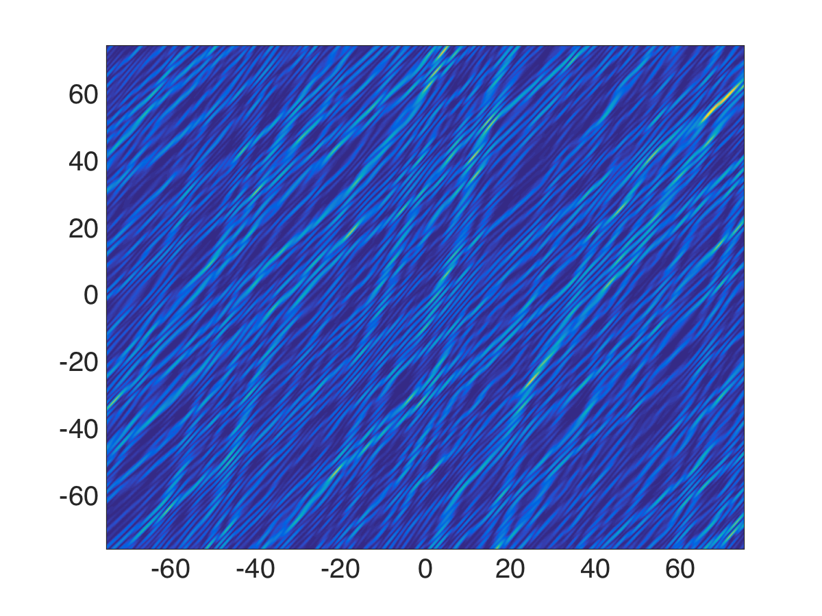
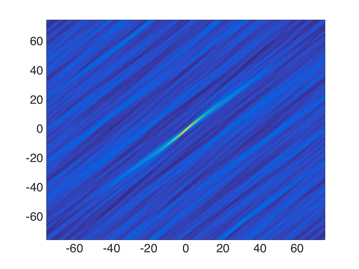
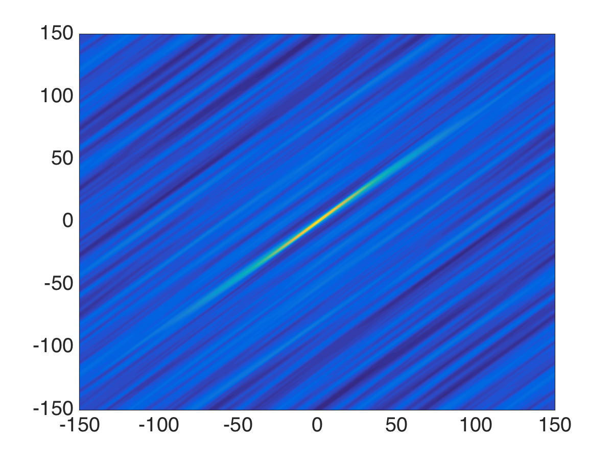
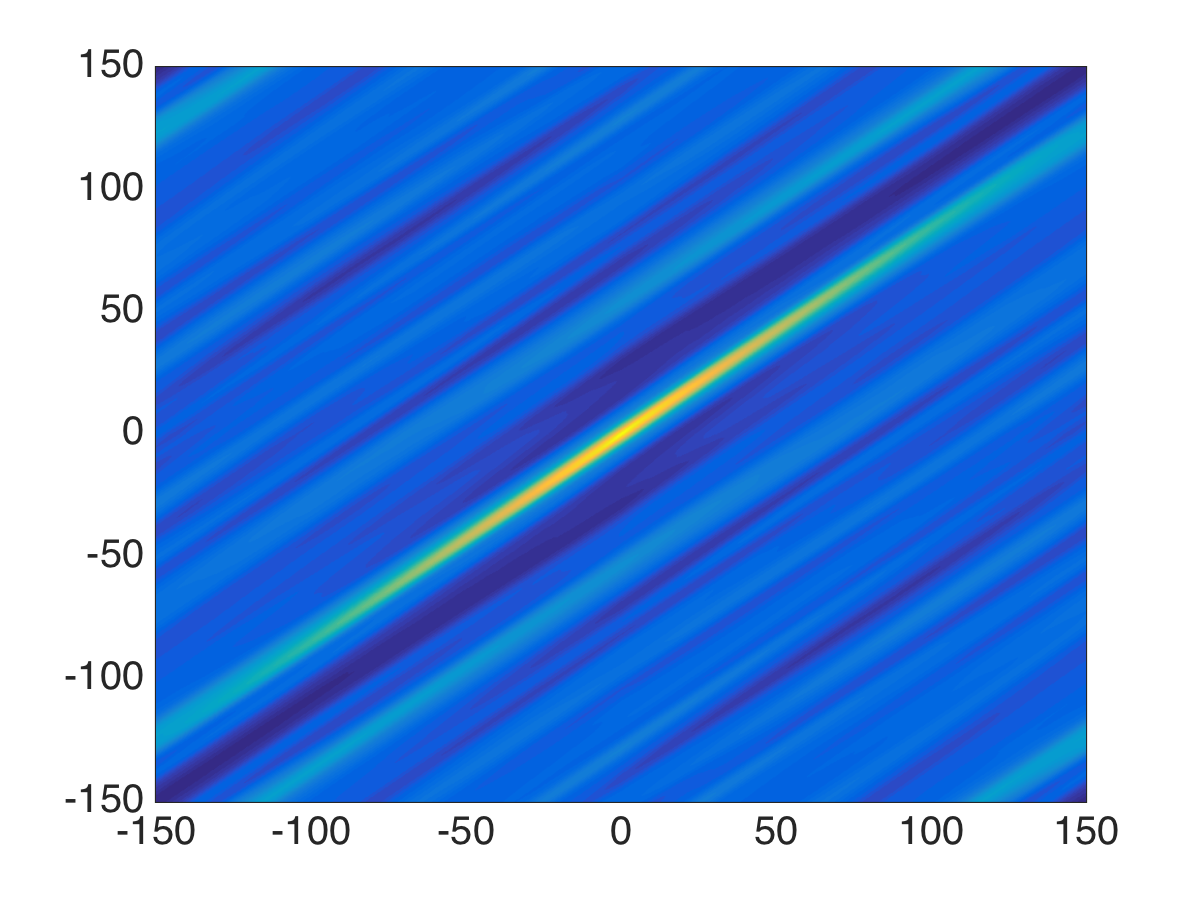
We present results for the following ratios of the radius of the particle and the wavelength: $a/\lambda=0.1,0.5,1$, and $2$. In the cases $a/\lambda\leq 0.5$ we consider an aperture with diameter $d_{A}=150\lambda$, and $900$ pixels, to obtain a resolution of $\lambda/6$. In the other two cases we have $d_{A}=300\lambda$ and the same number of pixels, to obtain a resolution of $\lambda/3$.

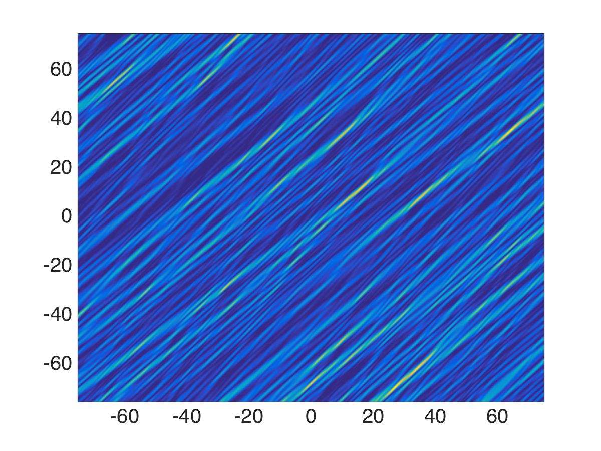
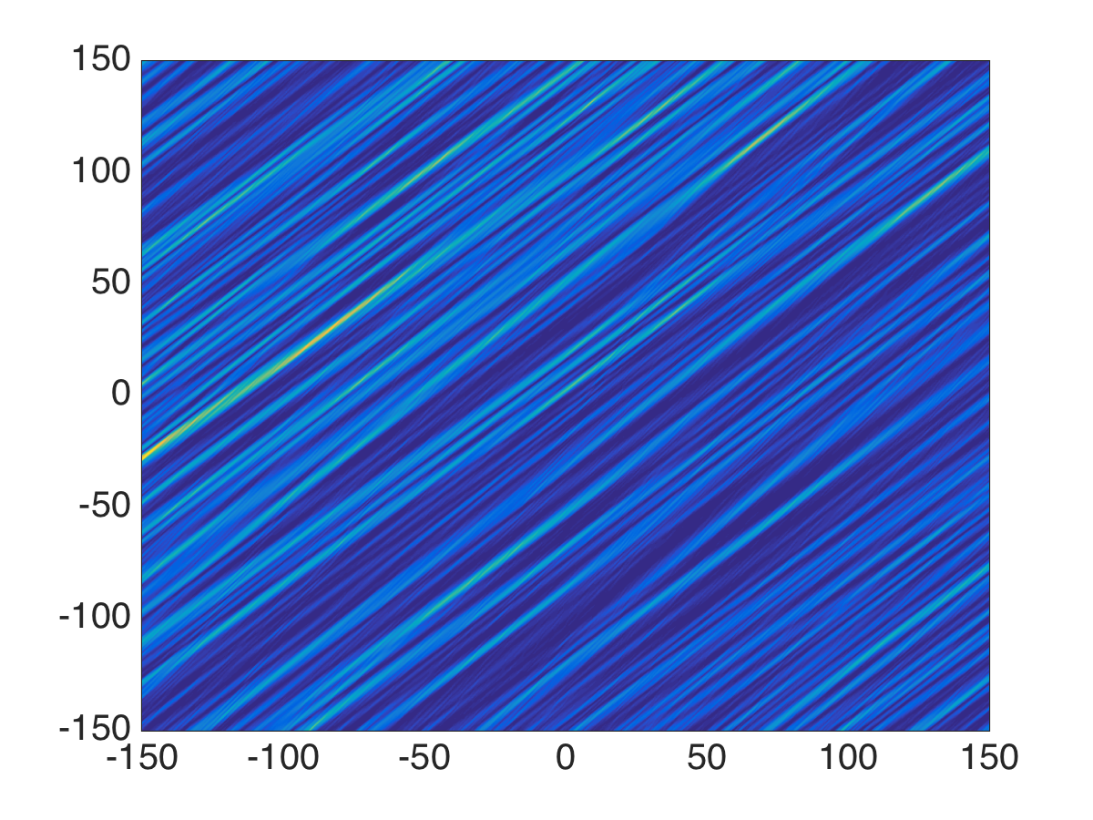
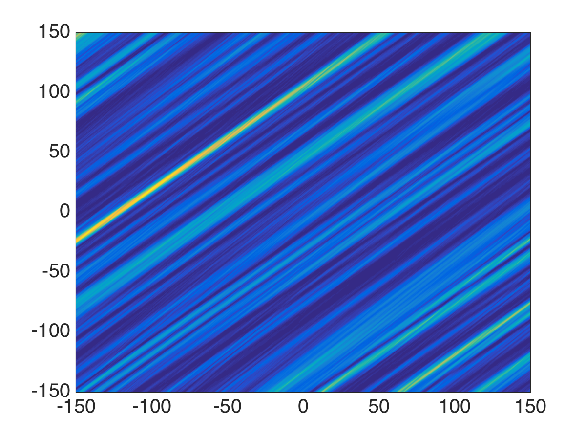
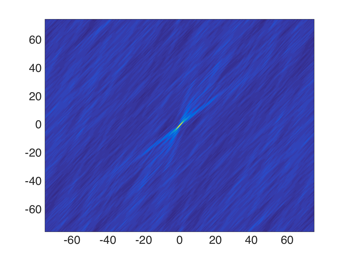
We display in Figure 3 the speckle pattern of the intensity at the first camera centered at $\vec{\itbf X}^{(1)}$, and the estimated correlation function (49) calculated as in (47), using FFT. We note the anisotropy of the decay of the correlation function, as discussed in section 4.2.

The matrices ${\bm{\mathfrak{U}}}^{(j)}$, for $j=1,\ldots,4$, are estimated as described in section 4.3, for the level set parameter $\mathfrak{L}=0.15$. The symmetric matrix ${\bf V}$ in the optimization (55) is represented by three search parameters: the two entries on the diagonal and the one off the diagonal. The minimization is solved with the MATLAB routine fmincon.

We display in the next table the eigenvalues $(\Lambda_{q}^{(1)})_{1\leq q\leq 3}$ of ${\bm{\mathfrak{U}}}^{(1)}$, for the four ratios $a/\lambda$. The eigenvalues of the other matrices have a similar behavior.

$a/\lambda$	$\Lambda_{1}^{(1)}$	$\Lambda_{2}^{(1)}$	$\Lambda_{3}^{(1)}$
0.1	29.49	1.14	-0.10
0.5	11.86	0.26	0.02
1	2.69	0.01	-0.05
2	0.5417	0.004	-0.02

Recall that $\Big{(}\Lambda_{j}^{(1)}\Big{)}^{-1/2}$, $j=1,2,3$, determine the semi-principal axes of the ellipsoid which approximates the level set of the correlation function, at level value $1-\mathfrak{L}$. These are proportional to the correlation lengths, and as stated in Propositions 2 and 4, the correlation lengths increase with the size of the particles. This is why $\Lambda_{1}^{(1)}$ is the largest when $a=0.1\lambda$.

The smallest eigenvalue $\Lambda_{3}^{(1)}$ is well separated from the others in the case $a/\lambda=0.1$, so we use Algorithm 6 to estimate the laser beam in this case. In all other cases the estimation is done using Algorithm 7 for two groups of cameras, and Algorithm 9 for $3$ or $4$ groups of cameras. We do not use Algorithm 6 for the case $a=0.5\lambda$, because the gap $\Lambda_{2}^{(2)}-\Lambda_{1}^{(1)}$ was smaller for the matrix ${\bm{\mathfrak{U}}}^{(2)}$.

The results obtained with the first two groups of cameras are in the next table, where we recall the estimation error quantifiers $\beta$ and $d$ are defined in (64) and (65). The angle $\beta$ is in degrees and the distance $d$ is in meters.

$a/\lambda$	$\beta$	$d$
0.1	$3.5^{o}$	$2.47$m
0.5	$30.5^{o}$	$9.27$m
1	$17.6^{o}$	$6.12$m
2	$12.6^{o}$	$3.94$m

We note that the best estimate is for the smallest particles. This is expected from scenario 1 discussed in section 4.4, because the eigenvectors ${\hat{\vec{\bm{\mathfrak{u}}}}}_{3}^{(j)}$ are robust to estimation errors, and approximate well the unit vectors normal to the planes defined by the centers of the cameras and the axis of the laser. The estimates for the larger particles are worse, with the case $a=2\lambda$ being the better one, as it is marginally in scenario 2 discussed in section 4.4, where the leading eigenvectors of ${\hat{\vec{\bm{\mathfrak{u}}}}}_{1}^{(j)}$, for $j=1,2$, are nearly orthogonal to the axis of the laser.

The results improve significantly when we use the three first groups of cameras, as shown in the next table. We only display the results for the larger particles, because Algorithm 9 terminates at Step 1 in the case $a=0.1\lambda$.

$a/\lambda$	$\beta$	$d$
0.5	$2.6^{o}$	$1.84$m
1	$2.9^{o}$	$2.42$m
2	$2.4^{o}$	$1.72$m

The results with all four groups of cameras are qualitatively the same, as shown below.

$a/\lambda$	$\beta$	$d$
0.5	$2.4^{o}$	$1.02$m
1	$0.9^{o}$	$0.57$m
2	$0.9^{o}$	$2.08$m

6 Summary

This paper introduces a novel algorithm for imaging a laser beam using measurements at CCD cameras that do not lie in the footprint of the beam. Motivated by the application of detection and characterization of high energy, continuous wave lasers in maritime atmospheres, we consider the light scattered away from the axis of the beam by small particles suspended in air (aerosols). We derive a model of the light intensity at the cameras using the Mie scattering theory for a Poisson cloud of spherical particles. This model displays the generic dependence of the speckle pattern of the intensity on the laser beam. By generic we mean that the conclusions extend to mixtures of particle sizes and shapes and to strong scattering regimes, as long as the cameras are not farther than a transport mean free path from the axis of the laser. The imaging algorithm is based on the behavior of the correlation function of the intensity, in particular on its anisotropic decay on length scales, called correlation lengths, which depend on the orientation of the axis of the laser. It estimates this correlation function using measurements at groups of three CCD cameras with a common center and apertures that lie in different planes. Two such groups of cameras are sufficient for imaging the laser beam in the case of either small or large particles with respect to the wavelength. For particles of general size, at least three groups of cameras are needed to obtain an accurate image. The theoretical results are validated with numerical simulations.

Appendix A The covariance function of the scattered field for small particles

We begin the proof of Proposition 2 with the model (9) of the scattered field and the approximation (10) of the Mie scattering kernel by the constant $\eta$ defined in (10),

$$u_{\rm s}(\vec{\itbf x})\approx{k^{2}\eta}\sum_{j}G(\vec{\itbf x},\vec{\itbf x}_{j})u_{\rm b}(\vec{\itbf x}_{j}).$$ (66)

Using the expressions (5) and (8) of the laser beam field $u_{\rm b}$ and the Green’s function $G$, and then taking expectations as described in (17), we obtain

$$\mathbb{E}\big{[} u_{\rm s}(\vec{\itbf x})]\approx\rho k^{2}\eta\int_{0}^{\infty}dz^{\prime}\int_{\mathbb{R}^{2}}d{\itbf x}^{\prime}\,{G}(\vec{\itbf x},\vec{\itbf x}^{\prime})u_{\rm b}(\vec{\itbf x}^{\prime})$$

$$=\frac{\rho k^{2}\eta}{4\pi}\int_{0}^{\infty}dz^{\prime}\int_{\mathbb{R}^{2}}d{\itbf x}^{\prime}\,\frac{r_{o}^{2}}{|\vec{\itbf x}-\vec{\itbf x}^{\prime}|R_{z^{\prime}}^{2}}\exp\Big{[}-\frac{|{\itbf x}^{\prime}|^{2}}{R_{z^{\prime}}^{2}}+(ik-k_{\rm d})(z^{\prime}+|\vec{\itbf x}-\vec{\itbf x}^{\prime}|)\Big{]}.$$ (67)

Here we decomposed $\vec{\itbf x}^{\prime}=({\itbf x}^{\prime},z^{\prime})$, with range coordinate $z^{\prime}>0$ along the axis of the beam and two-dimensional cross-range vector ${\itbf x}^{\prime}$. In our scaling regime $kz^{\prime}\sim{L_{z}}/{\lambda}\gg 1,$ and the mean zero result (23) follows from the Riemann-Lebesgue lemma, due to the rapid phase $\exp(ikz^{\prime})$ in equation (67).

Next we let $\vec{\itbf x}_{1}=\vec{\itbf X}+\vec{\itbf x}/2$ and $\vec{\itbf x}_{2}=\vec{\itbf X}-\vec{\itbf x}/2,$ and calculate the covariance function

$$\mathbb{E}\big{[} u_{\rm s}(\vec{\itbf x}_{1})\overline{u_{\rm s}}(\vec{\itbf x}_{2})\big{]}=\eta^{2}k^{4}\rho\int_{0}^{\infty}dz^{\prime}\int_{\mathbb{R}^{2}}d{\itbf x}^{\prime}\,{G}(\vec{\itbf x}_{1},\vec{\itbf x}^{\prime})\overline{{G}(\vec{\itbf x}_{2},\vec{\itbf x}^{\prime})}|u_{\rm b}(\vec{\itbf x}^{\prime})|^{2}$$

$$=\frac{\eta^{2}k^{4}\rho}{16\pi^{2}}\int_{0}^{\infty}dz^{\prime}\int_{\mathbb{R}^{2}}d{\itbf x}^{\prime}\,\frac{r_{o}^{4}}{|\vec{\itbf x}_{1}-\vec{\itbf x}^{\prime}||\vec{\itbf x}_{2}-\vec{\itbf x}^{\prime}||R_{z^{\prime}}|^{4}}\exp\Big{(}-\frac{2r_{o}^{2}|{\itbf x}^{\prime}|^{2}}{|R_{z^{\prime}}|^{4}}-2k_{\rm d}z^{\prime}\Big{)}$$

$$\quad\times\exp\Big{[}ik\big{(}|\vec{\itbf x}_{1}-\vec{\itbf x}^{\prime}|-|\vec{\itbf x}_{2}-\vec{\itbf x}^{\prime}|\big{)}-k_{\rm d}\big{(}|\vec{\itbf x}_{1}-\vec{\itbf x}^{\prime}|+|\vec{\itbf x}_{2}-\vec{\itbf x}^{\prime}|\big{)}\Big{]},$$ (68)

where we used that

$${\rm Re}\left(\frac{1}{R_{z^{\prime}}^{2}}\right)=\frac{r_{o}^{2}}{|R_{z^{\prime}}|^{4}}.$$

We have

$$k\big{(}|\vec{\itbf x}_{1}-\vec{\itbf x}^{\prime}|-|\vec{\itbf x}_{2}-\vec{\itbf x}^{\prime}|\big{)} =k\Big{(}\Big{|}\vec{\itbf X}-\vec{\itbf x}^{\prime}+\frac{\vec{\itbf x}}{2}\Big{|}-\Big{|}\vec{\itbf X}-\vec{\itbf x}^{\prime}-\frac{\vec{\itbf x}}{2}\Big{|}\Big{)}$$

$$=k\vec{\itbf x}\cdot\frac{(\vec{\itbf X}-\vec{\itbf x}^{\prime})}{|\vec{\itbf X}-\vec{\itbf x}^{\prime}|}+O\Big{(}\frac{k|\vec{\itbf x}|^{3}}{|\vec{\itbf X}-\vec{\itbf x}^{\prime}|^{2}}\Big{)},$$ (69)

where the residual is negligible if

$$|\vec{\itbf x}|\ll\lambda^{1/3}L_{\itbf x}^{2/3},$$ (70)

which we assume. We also have the approximations for the amplitude factors

$$\frac{1}{|\vec{\itbf x}_{1}-\vec{\itbf x}^{\prime}|}\approx\frac{1}{|\vec{\itbf x}_{2}-\vec{\itbf x}^{\prime}|}\approx\frac{1}{|\vec{\itbf X}-\vec{\itbf x}^{\prime}|}\approx\frac{1}{\sqrt{|{\itbf X}|^{2}+(Z-z^{\prime})^{2}}},$$ (71)

and

$$k_{\rm d}\big{(}2z^{\prime}+|\vec{\itbf x}_{1}-\vec{\itbf x}^{\prime}|+|\vec{\itbf x}_{2}-\vec{\itbf x}^{\prime}|\big{)}\approx 2k_{\rm d}[z^{\prime}+\sqrt{|{\itbf X}|^{2}+(Z-z^{\prime})^{2}}]\approx 2k_{\rm d}(z^{\prime}+|Z-z^{\prime}|),$$ (72)

by assumption (15) and the scaling relations

$$|{\itbf x}^{\prime}|\sim r_{o}\ll|{\itbf X}|\sim L_{\itbf x}\ll Z\sim L_{z}.$$

Substituting (69), (71), and (72) into equation (68) we obtain

$$\mathbb{E}\big{[}u_{\rm s}(\vec{\itbf x}_{1})\overline{u_{\rm s}}(\vec{\itbf x}_{2})\big{]}\approx \frac{\eta^{2}k^{4}\rho}{16\pi^{2}}\int_{0}^{\infty}dz^{\prime}e^{-2k_{\rm d}(z^{\prime}+|Z-z^{\prime}|)}\int_{\mathbb{R}^{2}}d{\itbf x}^{\prime}\frac{r_{o}^{4}}{\big{[}|{\itbf X}|^{2}+(Z-z^{\prime})^{2}\big{]}|R_{z^{\prime}}|^{4}}$$

$$\times\exp\Big{[}-\frac{2r_{o}^{2}|{\itbf x}^{\prime}|^{2}}{|R_{z^{\prime}}|^{4}}+ik\frac{({\itbf X}-{\itbf x}^{\prime})\cdot{\itbf x}+(Z-z^{\prime})z}{\sqrt{|{\itbf X}-{\itbf x}^{\prime}|^{2}+(Z-z^{\prime})^{2}}}\Big{]}.$$ (73)

The integrand in this equation is large for $|{\itbf x}^{\prime}|\lesssim r_{o}$ and we have $|{\itbf X}|\sim L_{\itbf x}$, so we can expand the phase as

$$k\frac{({\itbf X}-{\itbf x}^{\prime})\cdot{\itbf x}+(Z-z^{\prime})z}{\sqrt{|{\itbf X}-{\itbf x}^{\prime}|^{2}+(Z-z^{\prime})^{2}}}= k\frac{{\itbf X}\cdot{\itbf x}+(Z-z^{\prime})z}{\sqrt{|{\itbf X}|^{2}+(Z-z^{\prime})^{2}}}$$

$$+k{\itbf x}^{\prime}\cdot\frac{[{\itbf X}\cdot{\itbf x}+(Z-z^{\prime})z]{\itbf X}-[|{\itbf X}|^{2}+(Z-z^{\prime})^{2}]{\itbf x}}{[|{\itbf X}|^{2}+(Z-z^{\prime})^{2}]^{3/2}}$$

$$+O\Big{(}k\frac{|{\itbf x}^{\prime}|^{2}|\vec{\itbf x}|}{|{\itbf X}|^{2}}\Big{)}.$$ (74)

Note that the residual is small if

$$|\vec{\itbf x}|\ll\lambda(L_{\itbf x}^{2}/r_{o}^{2}),$$ (75)

which we assume. This allows us to integrate over ${\itbf x}^{\prime}$ in (73) and we obtain

$$\mathbb{E}\big{[}u_{\rm s}(\vec{\itbf x}_{1})\overline{u_{\rm s}}(\vec{\itbf x}_{2})\big{]}\approx \frac{\eta^{2}k^{4}\rho r_{o}^{2}}{32\pi}\int_{0}^{\infty}dz^{\prime}\frac{e^{-2k_{\rm d}(z^{\prime}+|Z-z^{\prime}|)}}{\big{[}|{\itbf X}|^{2}+(Z-z^{\prime})^{2}\big{]}}$$

$$\times\exp\Big{[}ik\frac{{\itbf X}\cdot{\itbf x}+(Z-z^{\prime})z}{\sqrt{|{\itbf X}|^{2}+(Z-z^{\prime})^{2}}}-\frac{k^{2}|R_{z^{\prime}}|^{4}{\cal Q}(\vec{\itbf x},\vec{\itbf X},z^{\prime})}{8r_{o}^{2}}\Big{]}dz^{\prime},$$ (76)

with

$${\cal Q}(\vec{\itbf x},\vec{\itbf X},z^{\prime})= \Big{|}\frac{[{\itbf X}\cdot{\itbf x}+(Z-z^{\prime})z]{\itbf X}-[|{\itbf X}|^{2}+(Z-z^{\prime})^{2}]{\itbf x}}{[|{\itbf X}|^{2}+(Z-z^{\prime})^{2}]^{3/2}}\Big{|}^{2}$$

$$= \frac{-({\itbf x}\cdot{\itbf X})^{2}|{\itbf X}|^{2}+z^{2}(Z-z^{\prime})^{2}|{\itbf X}|^{2}+|{\itbf x}|^{2}[|{\itbf X}|^{2}+(Z-z^{\prime})^{2}]^{2}}{[|{\itbf X}|^{2}+(Z-z^{\prime})^{2}]^{3}}$$

$$-\frac{2({\itbf x}\cdot{\itbf X})[{\itbf x}\cdot{\itbf X}+(Z-z^{\prime})z](Z-z^{\prime})^{2}}{[|{\itbf X}|^{2}+(Z-z^{\prime})^{2}]^{3}}.$$

Now let us change variables

$$z^{\prime}=Z-|{\itbf X}|\zeta,\quad\zeta\in\Big{(}-\infty,\frac{Z}{|{\itbf X}|}\Big{)},$$ (77)

and use that $Z/|{\itbf X}|\gg 1$ to extend the $\zeta$ interval to the real line. Equation (76) becomes

$$\mathbb{E}\big{[}u_{\rm s}(\vec{\itbf x}_{1})\overline{u_{\rm s}}(\vec{\itbf x}_{2})\big{]}\approx \frac{\eta^{2}k^{4}\rho r_{o}^{2}e^{-2k_{\rm d}Z}}{32\pi|{\itbf X}|}\int_{-\infty}^{\infty}\frac{e^{-2k_{\rm d}|{\itbf X}|(|\zeta|-\zeta)}}{1+\zeta^{2}}$$

$$\times\exp\Big{(}ik\frac{\hat{{\itbf X}}\cdot{\itbf x}+\zeta z}{\sqrt{1+\zeta^{2}}}-\frac{k^{2}|R_{{}_{Z-|{\itbf X}|\zeta}}|^{4}\tilde{\cal Q}(\vec{\itbf x},\hat{\itbf X},\zeta)}{8|{\itbf X}|^{2}r_{o}^{2}}\Big{)}d\zeta,$$ (78)

where $\hat{{\itbf X}}={\itbf X}/|{\itbf X}|$ and

$$\tilde{\cal Q}(\vec{\itbf x},\hat{\itbf X},\zeta)=\frac{-({\itbf x}\cdot\hat{\itbf X})^{2}(1+2\zeta^{2})+|{\itbf x}|^{2}(1+\zeta^{2})^{2}+z^{2}\zeta^{2}-2({\itbf x}\cdot\hat{\itbf X})z\zeta^{2}}{(1+\zeta^{2})^{3}}.$$

We can simplify this result further, by noting that since $1/(1+\zeta^{2})$ is integrable, only the terms with $|\zeta|=O(1)$ contribute to value of the integral (78), and we can approximate

$$|R_{{}_{Z-|{\itbf X}|\zeta}}|\approx r_{o},\qquad e^{-2k_{\rm d}|{\itbf X}|(|\zeta|-\zeta)}\approx 1,$$

by the scaling assumptions (14) and (15). Furthermore, $|\hat{{\itbf X}}\cdot{\itbf x}|$ and $|z|$ should be at most of order $\lambda$ otherwise the integral in (78) averages out by the Riemann-Lebesgue lemma, and in these conditions

$$\frac{k^{2}r_{o}^{2}}{8|{\itbf X}|^{2}}\tilde{\cal Q}(\vec{\itbf x},\hat{\itbf X},\zeta)=\frac{k^{2}r_{o}^{2}}{8|{\itbf X}|^{2}}|\hat{{\itbf X}}^{\perp}\cdot{\itbf x}|^{2}+o(1),$$

using the orthonormal basis $\{\hat{\itbf X},\hat{{\itbf X}}^{\perp}\}$ in the cross-range plane, so that

$$\mathbb{E}\big{[}u_{\rm s}(\vec{\itbf x}_{1})\overline{u_{\rm s}}(\vec{\itbf x}_{2})\big{]}\approx \frac{\eta^{2}k^{4}\rho r_{o}^{2}e^{-2k_{\rm d}Z}}{32\pi|{\itbf X}|}\int_{-\infty}^{\infty}\frac{1}{1+\zeta^{2}}$$

$$\times\exp\Big{(}ik\frac{\hat{{\itbf X}}\cdot{\itbf x}+\zeta z}{\sqrt{1+\zeta^{2}}}-\frac{k^{2}r_{o}^{2}|\hat{{\itbf X}}^{\perp}\cdot{\itbf x}|^{2}}{8|{\itbf X}|^{2}(1+\zeta^{2})}\Big{)}d\zeta.$$ (79)

Equations (24-25) follow after one more change of variables,

$$\zeta/\sqrt{1+\zeta^{2}}=\cos\alpha.$$ (80)

Note that this result shows that the covariance function, as a function of $\vec{\itbf x}$, has the form of an anisotropic peak centered at ${\bf 0}$ with radii of the order of $\lambda$ in the $z$- and $\hat{{\itbf X}}$-direction, and of the order of $\lambda|{\itbf X}|/r_{o}$ in the $\hat{{\itbf X}}^{\perp}$-direction. In order to see this peak, the radius of the camera should be ideally larger than $\lambda|{\itbf X}|/r_{o}$. If it is not as large, then the elongated peak will extend to the boundary of the domain.

Note also that (70) and (75) are readily fulfilled for $|\vec{\itbf x}|\lesssim\lambda$. When the diameter $d_{A}$ is larger than $\lambda|{\itbf X}|/r_{o}$, these conditions are fulfilled for all $\vec{\itbf x}$ in the peak of the covariance function if they hold for all $|\vec{\itbf x}|\leq\lambda L_{\itbf x}/r_{o}$, which happens if $(\lambda L_{\itbf x}/r_{o})^{3}\ll\lambda L_{\itbf x}^{2}$ and $\lambda L_{\itbf x}/r_{o}\ll\lambda(L_{\itbf x}^{2}/r_{o}^{2})$. This imposes the additional condition $\lambda^{2}L_{\itbf x}\ll r_{o}^{3}$.

Appendix B Proof of the Gaussian summation rule

We prove here that in our scaling regime the fourth order moments of the scattered field satisfy approximately the Gaussian summation rule. This gives the result stated in Proposition 3.

Let $\vec{\itbf x}_{1}=\vec{\itbf X}+\vec{\itbf x}/2$ and $\vec{\itbf x}_{2}=\vec{\itbf X}-\vec{\itbf x}/2$ be two points in the camera, and use equation (20) to write the second moment of the intensity

$$\mathbb{E}\big{[}|u_{\rm s}(\vec{\itbf x}_{1})|^{2}|{u_{\rm s}}(\vec{\itbf x}_{2})|^{2}\big{]} =\mathbb{E}\big{[}|u_{\rm s}(\vec{\itbf x}_{1})|^{2}\big{]}\mathbb{E}\big{[}|{u_{\rm s}}(\vec{\itbf x}_{2})|^{2}\big{]}+\big{|}\mathbb{E}\big{[}u_{\rm s}(\vec{\itbf x}_{1})\overline{u_{\rm s}}(\vec{\itbf x}_{2})\big{]}\big{|}^{2}$$

$$+\big{|}\mathbb{E}\big{[}u_{\rm s}(\vec{\itbf x}_{1}){u_{\rm s}}(\vec{\itbf x}_{2})\big{]}\big{|}^{2}+\mathcal{R}.$$ (81)

Here $\mathcal{R}$ is the residual given by the last term in (20),

$$\mathcal{R} =\rho\eta^{4}k^{8}\int_{0}^{\infty}dz^{\prime}\int_{\mathbb{R}^{2}}d{\itbf x}^{\prime}|{G}(\vec{\itbf x}_{1},\vec{\itbf x}^{\prime})|^{2}|{G}(\vec{\itbf x}_{2},\vec{\itbf x}^{\prime})|^{2}|u_{\rm b}(\vec{\itbf x}^{\prime})|^{4}$$

$$\approx\frac{\rho\eta^{4}k^{8}}{(4\pi)^{4}}\int_{0}^{\infty}dz^{\prime}\int_{\mathbb{R}^{2}}d{\itbf x}^{\prime}\frac{e^{-4k_{\rm d}(z^{\prime}+|Z-z^{\prime}|)}}{[|{\itbf X}|^{2}+(Z-z^{\prime})^{2}]^{2}}\frac{r_{o}^{8}}{|R_{z^{\prime}}|^{8}}\exp\Big{(}-\frac{4r_{o}^{2}|{\itbf x}^{\prime}|^{2}}{|R_{z^{\prime}}|^{4}}\Big{)}$$

$$=\frac{\rho\eta^{4}k^{8}r_{o}^{6}}{4^{5}\pi^{3}}\int_{0}^{\infty}dz^{\prime}\frac{e^{-4k_{\rm d}(z^{\prime}+|Z-z^{\prime}|)}}{[|{\itbf X}|^{2}+(Z-z^{\prime})^{2}]^{2}|R_{z^{\prime}}|^{4}},$$

where we used the same approximation as in (72). With the change of variables (77), and using that $Z/|{\itbf X}|\gg 1$, we estimate the residual by

$$\mathcal{R}\approx\frac{\rho\eta^{4}k^{8}r_{o}^{2}e^{-4k_{\rm d}Z}}{4^{5}\pi^{3}|{\itbf X}|^{3}}\int_{-\infty}^{\infty}\frac{1}{(1+\zeta^{2})^{2}}d\zeta=\frac{\rho\eta^{4}k^{8}r_{o}^{2}e^{-4k_{\rm d}Z}}{2^{11}\pi^{2}|{\itbf X}|^{3}}.$$

Let us compare ${\mathcal{R}}$ with the first two terms in (81), which are of the same order, estimated from equation (26),

$$\big{|}\mathbb{E}\big{[}u_{\rm s}(\vec{\itbf x}_{1})\overline{u_{\rm s}}(\vec{\itbf x}_{2})\big{]}\big{|}^{2}\sim\mathbb{E}\big{[}|u_{\rm s}(\vec{\itbf x}_{1})|^{2}\big{]}\mathbb{E}\big{[}|{u_{\rm s}}(\vec{\itbf x}_{2})|^{2}\big{]}\approx\left(\frac{\eta^{2}k^{4}\rho r_{o}^{2}e^{-2k_{\rm d}Z}}{32|{\itbf X}|}\right)^{2}.$$

We obtain that

$$\frac{\mathcal{R}}{\mathbb{E}\big{[}|u_{\rm s}(\vec{\itbf x}_{1})|^{2}\big{]}\mathbb{E}\big{[}|{u_{\rm s}}(\vec{\itbf x}_{2})|^{2}\big{]}}\approx\frac{1}{2\pi^{2}\rho r_{o}^{2}|{\itbf X}|}\ll 1,$$ (82)

because in our scaling

$$\rho r_{o}^{2}|{\itbf X}|=\frac{r_{o}^{2}|{\itbf X}|}{\ell^{3}}\gg 1.$$ (83)

Therefore, the residual is negligible in (81) and the covariance is given by

$${\rm Cov}\big{(}|u_{\rm s}(\vec{\itbf x}_{1})|^{2},|{u_{\rm s}}(\vec{\itbf x}_{2})|^{2}\big{)}\approx\big{|}\mathbb{E}\big{[}u_{\rm s}(\vec{\itbf x}_{1})\overline{u_{\rm s}}(\vec{\itbf x}_{2})\big{]}\big{|}^{2}+\big{|}\mathbb{E}\big{[}u_{\rm s}(\vec{\itbf x}_{1}){u_{\rm s}}(\vec{\itbf x}_{2})\big{]}\big{|}^{2}.$$ (84)

It remains to show that the last term in (84) is small. We have from the model (9) and equation (17) that

$$\mathbb{E}\big{[} u_{\rm s}(\vec{\itbf x}_{1}){u_{\rm s}}(\vec{\itbf x}_{2})\big{]}=\eta^{2}k^{4}\rho\int_{0}^{\infty}dz^{\prime}\int_{\mathbb{R}^{2}}d{\itbf x}^{\prime}\,{G}(\vec{\itbf x}_{1},\vec{\itbf x}^{\prime}){{G}(\vec{\itbf x}_{2},\vec{\itbf x}^{\prime})}|u_{\rm b}(\vec{\itbf x}^{\prime})|^{2}$$

$$=\frac{\eta^{2}k^{4}\rho}{16\pi^{2}}\int_{0}^{Z_{\rm P}}dz^{\prime}\int_{\mathbb{R}^{2}}d{\itbf x}^{\prime}\,\frac{r_{o}^{4}}{|\vec{\itbf x}_{1}-\vec{\itbf x}^{\prime}||\vec{\itbf x}_{2}-\vec{\itbf x}^{\prime}||R_{z^{\prime}}|^{4}}\exp\Big{[}-\frac{2r_{o}^{2}|{\itbf x}^{\prime}|^{2}}{|R_{z^{\prime}}|^{4}}+2(ik-k_{\rm d})z^{\prime}\Big{]}$$

$$\times\exp\Big{[}ik\big{(}|\vec{\itbf x}_{1}-\vec{\itbf x}^{\prime}|+|\vec{\itbf x}_{2}-\vec{\itbf x}^{\prime}|\big{)}-k_{\rm d}\big{(}|\vec{\itbf x}_{1}-\vec{\itbf x}^{\prime}|+|\vec{\itbf x}_{2}-\vec{\itbf x}^{\prime}|\big{)}\Big{]}.$$ (85)

This expression contains very large phases: $2kz^{\prime}\gg 1$ and $k\big{(}|\vec{\itbf x}_{1}-\vec{\itbf x}^{\prime}|+|\vec{\itbf x}_{2}-\vec{\itbf x}^{\prime}|\big{)}\gg 1$, so the result is small after integration, by the Riemann-Lebesgue lemma. The result stated in Proposition 3 follows.

References

- [1] M. Abramowitz and I. Stegun, Handbook of mathematical functions, Dover Publications, New York, 1965.
- [2] L. Borcea and J. Garnier, Derivation of a one-way radiative transfer equation in random media, Phys. Rev. E, 93, 022115 (2016).
- [3] J.-P. Cariou, Off-axis detection of pulsed laser beams: simulation and measurements in the lower atmosphere, Proc. SPIE 5086, Laser Radar Technology and Applications VIII, 129 (August 22, 2003).
- [4] S. Chandrasekhar, Radiative Transfer, Dover, New York, 1960.
- [5] J. Garnier and K. Sølna, Wave backscattering by point scatterers in the random paraxial regime, SIAM Multiscale Model. Simul., 12, 1309-1334 (2014).
- [6] F. Hanson and I. Bendall, Off-axis laser beam imaging and characterization with two cameras, Appl. Opt., 52, 5342-5347 (2013).
- [7] F. Hanson, I. Bendall, C. Deckard, and H. Haidar, Off-axis detection and characterization of laser beams in the maritime atmosphere, Appl. Opt., 50, 3050-3056 (2011).
- [8] T. L. Hayden and J. Wells, Approximation by matrices positive definite in a subspace, Linear Algebra and its Applications, 109, 115-130 (1988).
- [9] A. Ishimaru, Wave propagation and scattering in random media, Academic Press, San Diego, 1978.
- [10] J. F. Kingsman, Poisson processes, Oxford University Press, Oxford, 1993.
- [11] O. Korotkova, S. Avramov-Zamurovic, R. Malek-Madani, and C. Nelson, Probability density function of the intensity of a laser beam propagating in the maritime environment, Opt. Express, 19, 20322-20331 (2011).
- [12] J. T. Kusmierczyk-Michulec, Ric (H.M.A.) Schleijpen, Influence of aerosols on off-axis laser detection capabilities, Atmospheric Optics: Models, Measurements, and Target-in-the-Loop Propagation III, edited by Stephen M. Hammel, Alexander M. J. van Eijk, Mikhail A. Vorontsov, Proc. of SPIE Vol. 7463, 74630E, 2009. doi: 10.1117/12.828534
- [13] L. Mandel and E. Wolf, Optical Coherence and Quantum Optics. Cambridge: Cambridge University Press, 1995.
- [14] B. N. Parlett, The Symmetric Eigenvalue Problem, SIAM, Philadelphia, 1998.
- [15] M. Roy, F. Reid, Off-axis laser detection model in coastal areas, Optical Engineering, 47, 086002 (2008).
- [16] W. G. Tam and A. Zardecki, Off-axis propagation of a laser beam in low visibility weather conditions, Appl. Opt., 19, 2822-2827 (1980).
- [17] H. C. van de Hulst, Light scattering by small particles, Dover Publications, New York, 1981.
- [18] A. M. J. van Eijk, J. T. Kusmierczyk-Michulec, J. P. Piazzola, The Advanced Navy Aerosol Model (ANAM): Validation of small-particle modes, Atmospheric Optics IV: Turbulence and Propagation, edited by Alexander M. J. van Eijk, Stephen M. Hammel, Proc. of SPIE Vol. 8161, 816108, 2011, SPIE. doi: 10.1117/12.896178
- [19] M. C. W. van Rossum and Th. M. Nieuwenhuizen, Multiple scattering of classical waves: microscopy, mesoscopy, and diffusion, Rev. Mod. Phys., 71, 313-371 (1999).
- [20] W.-D. Wei, X.-Q. Sun, X.-J. Sun, Technical analysis on correlation detection of off-axis scattering of pulsed laser, 2012 International Conference on Computer Science and Information Processing (CSIP), pp. 271-274, 2012, IEEE.