Chemical reaction-controlled phase separated drops:
Formation, size selection, and coarsening

Abstract

Phase separation under non-equilibrium conditions is exploited by biological cells to organize their cytoplasm but remains poorly understood as a physical phenomenon. Here, we study a ternary fluid model in which phase-separating molecules can be converted into soluble molecules, and vice versa, via chemical reactions. We elucidate using analytical and simulation methods how drop size, formation, and coarsening can be controlled by the chemical reaction rates, and categorize the qualitative behavior of the system into distinct regimes. Ostwald ripening arrest occurs above critical reaction rates, demonstrating that this transition belongs entirely to the non-equilibrium regime. Our model is a minimal representation of the cell cytoplasm.

Phase separation is a ubiquitous phenomenon in our physical world, ranging from cloud formation to oil drop formation in water Bray (2002). Recently, it is also realised that phase separation is exploited in the cell cytoplasmic organization in the formation of non-membrane bound organelles called ribonucleoprotein (RNP) granules Brangwynne (2011); Hyman et al. (2014). RNP granules are a diverse set of structures that play important roles in the functioning of the cell, from RNA processing and stress response Anderson et al. (2009); Protter and Parker (2016), to cell division Zwicker et al. (2014) and germ line specification Brangwynne et al. (2009); Voronina et al. (2011). However, the mechanisms enabling the rapid and controlled assembly and disassembly of RNP granules have only begun to be investigated. Chemical reactions, e.g., in the form of ATP-driven enzymatic reactions that convert one protein state to another (e.g., unphosphorylated to phosphorylated) are prime candidates for the cell to manifest controlled phase separation. For instance, such a scheme has been proposed as a mean to induce localised phase separation in the C. elegans. embryo Lee et al. (2013); Saha et al. (2016); Weber et al. (2017), and to organise the centrosomes prior to cell division Zwicker et al. (2014). However the physics of non-equilibrium phase separation driven by chemical reactions has only started to be investigated. For instance, non-equilibrium processes have been discussed in the context of lipid domains in plasma membranes Turner et al. (2005); Fan et al. (2008). More recently, it has been realised that although in equilibrium phase separation, a multi-drop, finite system will invariably coarsen to a single condensed drop via Ostwald ripening, chemical reactions can arrest this ripening process completely in a binary fluid Glotzer et al. (1995); Zwicker et al. (2015). Here, we categorize comprehensively and under general conditions, how unimolecular reactions that convert a two-state molecule between a phase-separating state and a soluble state can control drop formation, coarsening, and size selection. We achieve this by generalizing and improving upon the assumptions adopted in Zwicker et al. (2015). Specifically, contrary to Zwicker et al. (2015), we analyse the regimes of large drops and non negligible supersaturation, include the presence of cytosol by going beyond the binary fluid restriction, and allow for arbitrary equilibrium concentrations inside and outside drops. Our model is arguably the minimal model relevant to the mechanism of chemical reaction-controlled phase separation in the cell cytoplasm.

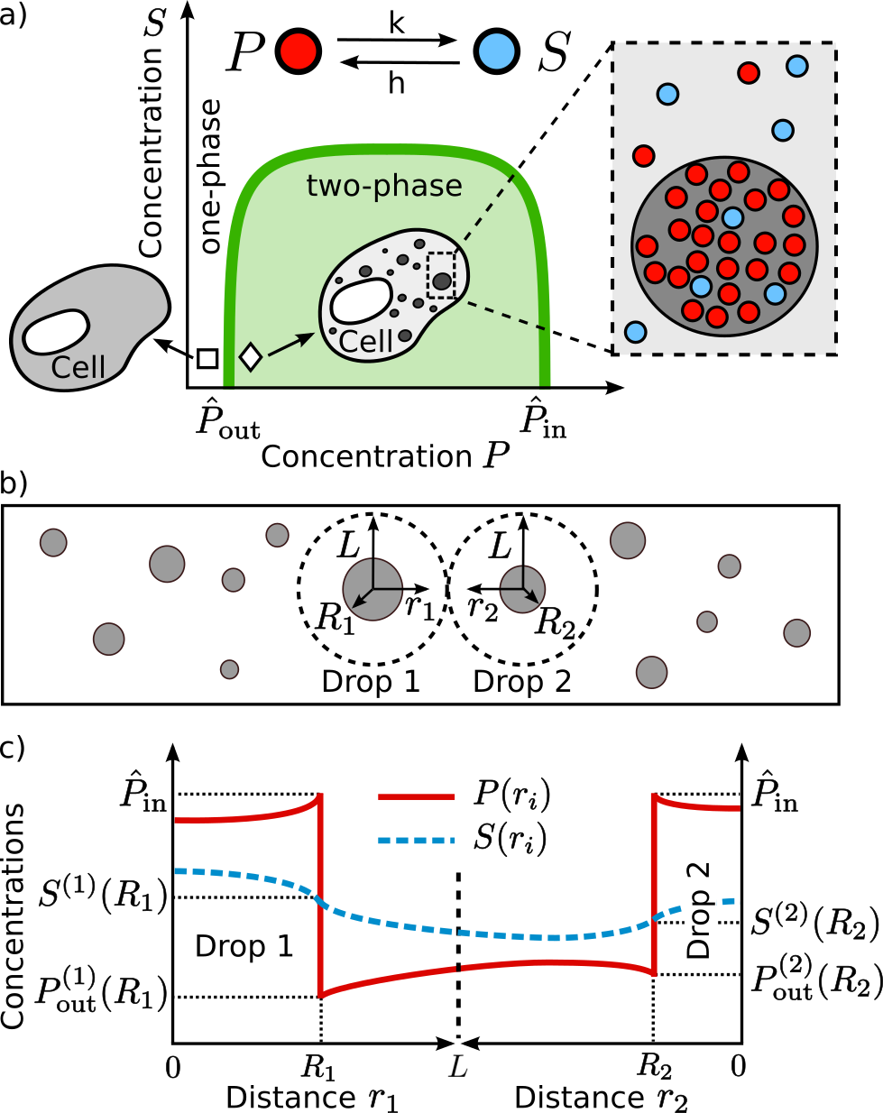
Figure 1: Model of cytoplasmic phase separation. a) The cell cytoplasm is modeled by a ternary fluid composed of phase-separating ($P$) and soluble ($S$) molecular states, and other cytoplasmic components ($C$). Chemical reactions convert $P$ into $S$ at the rate $k$, and $S$ into $P$ at the rate $h$ (Eq. (1)). At equilibrium ($k=h=0$), the system is well mixed (‘$\square$’) if the concentrations of $P$ and $S$ lie outside the phase boundary (green line in the phase diagram), and the system phase separates otherwise (‘$\lozenge$’). In the latter case, we assume that $S$ does not phase separate and remains homogeneous. b) A multi-drop system with drop number density $\rho$ is studied by considering two interacting subsystems ($i=1,2$) of radius $L=[3/(4\pi\rho)]^{1/3}$, each having a drop of radius $R_{i}$ in their center. c) Schematics of the concentration profiles of $P$ and $S$ in the subsystems when chemical reactions are present ($k,h>0$, Eqs. (8),(9)). At the subsystems’ boundaries ($r_{i}=L$) the profiles and their derivatives are matched by assumption (Eq. (7)).

Our ternary mixture consists of two molecular states, one phase-separating ($P$) and one soluble ($S$), plus the solvent or cytosol ($C$). States $P$ and $S$ can be converted into each other by the chemical reactions

$$\ce{P<=>[k][h]S}$$ (1)

where $k$ and $h$ are the reaction rate constants. The non-equilibrium nature of these reactions lies in the fact that both reaction rates are independent of the local concentrations and thus have to be driven by free energy consumption. In the context of the cell, these reactions can be, e.g., ATP-driven post-transcriptional protein modifications Alberts et al. (2008), that affect protein phase-separating behavior. For example, the phase separation of intrinsically disordered proteins can be regulated via their phosphorylation/dephosphorylation Li et al. (2012); Bah and Forman-Kay (2016).

At equilibrium ($k,h=0$), a finite system will inevitably coarsen via Ostwald ripening Lifshitz and Slyozov (1961) and drop coalescence Siggia (1979). Here, we assume that drop diffusion is negligible so we will focus exclusively on the Ostwald ripening. In the cell context, this is motivated by the strong suppression of macromolecular diffusion in the cell cytoplasm Weiss et al. (2004). Ostwald ripening results from two effects: 1) the Gibbs-Thomson relation dictating that for a drop of size $R$, the concentrations of solute inside and outside the drop next to the interface are $\hat{P}_{\rm in}$ and $\hat{P}_{\rm out}\left(1+l_{c}/R\right)$ respectively, where $l_{c}$ is the capillary length and $\hat{P}_{\rm in/out}$ are the equilibrium phase coexistence concentrations (see Fig. 1a)); and 2) the concentration profile of the solute in the dilute phase is given by the steady-state solution to the diffusion equation (the quasi-static assumption). These two effects combined lead to a diffusive flux of solute from small drops to big drops Lifshitz and Slyozov (1961).

When chemical reactions are switched on, we assume that local thermal equilibrium remains valid so that the interface boundary conditions for $P$ are unchanged . $S$ is considered inert to phase separation in the sense that its concentration profile is continuous across the interface . In addition, we assume that the concentration profiles inside and outside the drops are given by:

$$\frac{\partial P_{\rm in/out}}{\partial t} = D\nabla^{2}P_{\rm in/out}-kP_{\rm in/out}+hS_{\rm in/out}$$ (2)

$$\frac{\partial S_{\rm in/out}}{\partial t} = D\nabla^{2}S_{\rm in/out}+kP_{\rm in/out}-hS_{\rm in/out}\ ,$$ (3)

where $P_{\rm in/out}$ and $S_{\rm in/out}$ denote the concentration profiles of $P$ and $S$ inside and outside drops with subscripts “in” and “out”, respectively. For simplicity, we assume the same diffusion coefficient $D$ for both species and in both phases.

To see why Ostwald ripening can be arrested in our ternary mixture, we will now provide an intuitive argument based on a similar consideration for binary mixtures Zwicker et al. (2015). We consider a homogeneous system of total solute concentration $\phi=P_{\rm tot}+S_{\rm tot}$ where $P_{\rm tot}$ $(S_{\rm tot})$ is the total concentration of $P$ $(S)$ in the system. If the supersaturation $\triangle=P_{\rm tot}-\hat{P}_{\rm out}$ is positive drops can be nucleated, initiating phase separation (Fig. 1a)). At small $\triangle$ the drop density is low and drops only interact with the far-field concentration. We focus only on the early growth regime so that the supersaturation $\triangle$ remains close to $P_{\rm tot}-\hat{P}_{\rm out}$: for a drop of radius $R$, the diffusive profile leads to an influx of $P$ into the drop at the rate Lifshitz and Slyozov (1961)

$$4\pi DR\left(\triangle-\frac{\hat{P}_{\rm out}l_{c}}{R}\right)\ .$$ (4)

At the same time, the chemical reactions inside the drop lead to a depletion of $P$ at the rate

$$\frac{4\pi R^{3}}{3}k\hat{P}_{\rm in}\ .$$ (5)

As $R$ increases, the depletion rate will eventually surpass the influx from the medium, so that the balance between Eqs. (4) and (5) leads to a steady-state radius. In the limit of large $R$ so that we can ignore the term $\hat{P}_{\rm out}l_{c}/R$ (but still small such that $\triangle\approx P_{\rm tot}-\hat{P}_{\rm out}$), the steady-state $R$ is

$$\sqrt{\frac{3D\triangle}{k\hat{P}_{\rm in}}}\ .$$ (6)

In other words, we expect that in a multi-drop system, the size of all drops are given by Eq. (6). We shall see that this regime in fact corresponds to the upper bound of stable $R$ in a multi-drop system (Fig. 3).

In our argument above, we have neglected the reverse reaction $S\to P$ and the the effect of the chemical reactions on the diffusive profiles, which, as we shall see, can significantly change the system’s behavior. We will now incorporate these effects into our analysis. We will also consider arbitrary supersaturations so that drops may be close to each other. As a result a far-field concentration may not exist, rendering the Lifshitz-Slyozov theory Lifshitz and Slyozov (1961) inapplicable. Consider a multi-drop system such that drops are on average a distance $2L$ apart where $L$ is of the order $\rho^{-1/3}$ with $\rho$ being the drop number density. For simplicity, we will first focus on two spherical subsystems of radius $L$, each having a spherical drop in their center (Fig. 1b)). We assume that the concentrations and their gradients at the boundaries of the two subsystems match (Fig. 1c)). The rational for this approximation is that in a multi-drop system, the actual boundary conditions are influenced by many neighbouring drops and we treat these fluctuating boundary conditions in a mean-field manner by assuming spherical symmetry around the drops. In other words, the concentration outside a drop depends only on the distance from the drop centre. Moreover it is assumed that the two-drop system is stable (unstable) if the full multi-drop system is stable (unstable). The validity of this approximation will be verified later using Monte Carlo simulations. The corresponding boundary conditions, besides the Gibbs-Thomson at the drops’ interfaces, are

$$\quad P_{\rm out}^{(1)}(L)=P_{\rm out}^{(2)}(L),\quad\nabla_{\mathbf{r}_{1}}P_{\rm out}^{(1)}|_{L}=-\nabla_{\mathbf{r}_{2}}P_{\rm out}^{(2)}|_{L}\ ,$$ (7)

and the same apply to $S_{\rm in/out}^{(i)}$. The subscript $i=1,2$ denotes the drop index. Note that we use two different coordinate systems $r_{1}$ and $r_{2}$, each having their respective drop’s center as the origin (Fig. 1b)).

Using the quasi-static approximation as in the equilibrium case, the steady-state concentration profiles of this two-drop system with radii $R_{1}$ and $R_{2}$, such that $R_{1}\approx R_{2}$, are SI :

$$P_{\rm in}^{(i)}(r_{i}) = \frac{I_{i}h}{k+h}+H^{(i)}_{\rm in}\frac{R_{i}}{r_{i}}\frac{\sinh(r_{i}/\xi)}{\sinh(R_{i}/\xi)}$$ (8)

$$P_{\rm out}^{(i)}(r_{i}) = \frac{Oh}{k+h}+H^{(i)}_{\rm out}\frac{R_{i}}{r_{i}}\left(A_{i}{\rm e}^{r_{i}/\xi}+B_{i}{\rm e}^{-r_{i}/\xi}\right).\$$ (9)

In the above, $A_{i},B_{i}$ are independent of $r_{i}$ and are given in SI , $I_{i}$, $O$ denote the combined concentration $P+S$ inside and outside the $i$-th drop, respectively, and are also independent of $r_{i}$. Furthermore, $H^{(i)}_{\rm in}\equiv\hat{P}_{\rm in}-I_{i}h/(k+h)$, $H^{(i)}_{\rm out}\equiv P^{(i)}_{\rm out}(R_{i})-Oh/(k+h)$, and $\xi\equiv\sqrt{D/(k+h)}$ is the concentration gradient length scale. The $S$ profiles are given by $S^{(i)}(r_{i})=I_{i}-P_{\rm in}^{(i)}(r_{i})$ for $r_{i}<R_{i}$ and $S^{(i)}(r_{i})=O-P_{\rm out}^{(i)}(r_{i})$ for $r_{i}>R_{i}$. Note that generally, $O$ is independent of $r$ only when $R_{1}=R_{2}$, which we have assumed to be true here as we will focus on the case $R_{1}\approx R_{2}$.

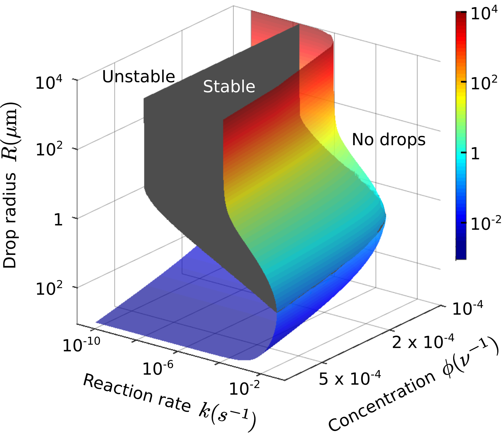
Figure 2: . The stability of a multi-drop system at fixed backward reaction rate $h$. The region of existence of a steady-state radius $R^{*}$ (solution of $g_{0}(R^{*})=0$, Eq. (12)) is controlled by the forward reaction rate $k$ and the total solute concentration $\phi$. In the region enclosed by the coloured outer surface, $R^{*}$ exists and depends on the drop number density $\rho$ which is not fixed in this figure. The steady-state is stable ($g_{1}(R^{*})<0$, Eq. (11)) above the black inner surface, and unstable ($g_{1}(R^{*})>0$) bellow this surface. Parameters: $h=10^{-2}s^{-1},~{}l_{c}=10^{-2}{\rm\mu m},~{}D=1{\rm\mu m^{2}s^{-1}},~{}\hat{P}_{\rm in}=5\times 10^{-2}{\nu^{-1}},~{}\hat{P}_{\rm out}=10^{-4}{\nu^{-1}}$, where $\nu$ is the molecular volume of $P$ and $S$ and can be chosen arbitrarily.

The volumetric growth rate of the $i$-th drop in this two-drop system is Zwicker et al. (2014)

$$G_{i}(R_{i},R_{j})=\frac{4\pi DR_{i}^{2}}{\hat{P}_{\rm in}-P_{\rm out}^{(i)}(R_{i})}\left(\left.\frac{{\rm d}P_{\rm out}^{(i)}}{{\rm d}r_{i}}\right|_{R_{i}^{+}}-\left.\frac{{\rm d}P_{\rm in}^{(i)}}{{\rm d}r_{i}}\right|_{R_{i}^{-}}\right).\$$ (10)

Given the drop growth rate above we can study the steady-state drop radius $R^{*}$ at which the two drops of the same size are in the steady-state ($G_{i}=0$).

We can also analyse its stability by calculating the drops’ growth rates upon perturbing their sizes: $R_{1}\mapsto R^{*}+\epsilon$ and $R_{2}\mapsto R^{*}-\epsilon$. Performing a linear stability analysis, we take $\epsilon\ll R^{*}$ and expand the growth rate with respect to $\epsilon$:

$$G_{1}(R_{1},R_{2})=g_{0}(R^{*})+g_{1}(R^{*})\epsilon+{\cal O}(\epsilon)\ .$$ (11)

Solving for $g_{0}(R^{*})=0$ gives the steady-state drop radius $R^{*}$ and the sign of $g_{1}(R^{*})$ indicates the stability of the system: coarsening will occur if $g_{1}>0$ while the system is stable if $g_{1}<0$. Using the profiles (8) & (9), we find

$$g_{0}(R^{*})=\frac{4\pi DR^{*}}{\hat{P}_{\rm in}-P_{\rm out}{(R^{*})}}\left[H_{\rm in}\left(1-\frac{R^{*}}{\xi}\coth{\frac{R^{*}}{\xi}}\right)\right.$$ (12)

$$\ \ \ \ \ \ -\left.H_{\rm out}\left(A\left(1-\frac{R^{*}}{\xi}\right)e^{\frac{R^{*}}{\xi}}+B\left(1+\frac{R^{*}}{\xi}\right)e^{-\frac{R^{*}}{\xi}}\right)\right]$$

with $H_{\rm in/out}\equiv H^{(i)}_{\rm in/out}(R_{1}=R_{2}=R^{*})$ and $A$ and $B$ are function of $R^{*}/\xi$ and $L/\xi$ SI . The expression of $g_{1}(R^{*})$ is more complicated and is shown in SI .

The surface plot in Fig. 2 shows for a fixed backward reaction rate $h$, the region of existence of the steady-state radius $R^{*}$, delimited by the coloured outer surface. Above the black inner surface, the system consists of stable monodisperse drops whose sizes are controlled by the rate $k$, the solute concentration $\phi$ and the drop number density $\rho$ (not fixed in Fig. 2). Outside the stable region but still within the outer surface, the monodisperse system is in an unstable steady-state and drops coarsen via Ostwald ripening. Outside the outer surface, drops always shrink.

Interestingly, there are qualitative changes in the system’s behaviour as $k$ varies with fixed $h$ as shown in Fig. 3, which describes multi-drop stability at fixed solute concentration $\phi$. When $k<k_{l}$ (blue arrow), the system is in the Lifshitz-Slyozov regime and coarsen (upward arrows), while for $k_{l}<k<k_{u}$ (green arrow), the system can be stable (grey region), with co-existing drops of radius determined by $\rho$. In other words, $k_{l}$ is the critical rate beyond which Ostwald ripening is arrested. Between $k_{u}$ and $k_{c}$ (black arrow), the system can also be stable, but with an upper bound on the radius. Beyond $k_{c}$, no drops can exist in the system as all drops evaporate (downward arrows).

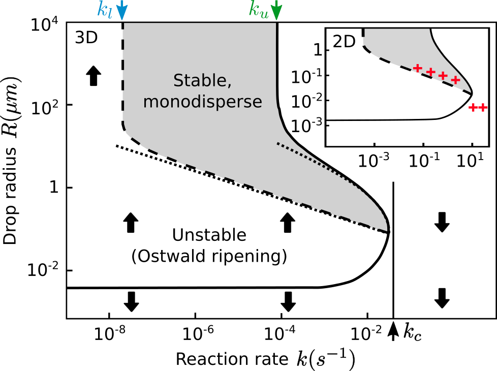
Figure 3: Stability diagram of a multi-drop system at fixed backward rate $h$ and fixed solute concentration $\phi$. A steady-state drop radius $R^{*}$ exists in the region enclosed by the continuous line and depends on the rate $k$ and the drop number density $\rho$. Outside this region no steady-states exist and drops dissolve (downward arrows). The lower part of this line represents the smallest possible drop, or nucleus. Outside the grey region but still within the continuous line the steady-state is unstable causing the average radius to increase (upward arrows). The stability-instability boundary ($g_{1}(R^{*})=0$) is shown with a dashed line. There is a good agreement between our analytical calculation and the numerical solutions for $k_{l},k_{u},k_{c}$. The analytical expressions for the upper bound radius $R_{u}$ (Eq. (13)) and the stability-instability boundary $R_{l}$ (Eq. (15)) in the small drop regime ($R^{*}\ll\xi$) are shown by the dotted lines. Parameters: $\phi=5\times 10^{-4}\nu^{-1},~{}\hat{P}_{\rm in}=10^{-1}\nu^{-1}$ and the rest are as in Fig. 2. Insert: Comparison between 2D Monte Carlo simulations and numerical solutions to the linear stability analysis. Simulation data are shown in red, note that the two rightmost crosses represent the size of the lattice site ($\sim 10^{-2}\rm{\mu m}$), i.e., there are no drops in the system. The region $k\approx k_{l}$ is also investigated in SI . See SI for the corresponding analysis in 2D and simulation details.

So far, our calculation has been based on our two-drop system with the mean-field matching assumption at the system boundaries. To test this assumption, we perform Monte Carlo simulations of our ternary model on a 2D lattice with multiple drops to detect the stability-instability boundary (black inner surface in Fig. 2 and dashed curve in Fig. 3) and compare the results with our predictions (see SI for simulation details.) The good agreements are shown in the inset of Fig. 3 and in SI .

We will now explain analytically the salient features of the stability diagram by focusing on distinct limits in the small supersaturation limit.

Upper bound on drop radius. We have seen that if $k_{u}<k<k_{c}$, there is an upper bound on the drop radius. We focus here on the regime $R^{*}\ll\xi$, which we will see is indeed the case when $k\gg k_{u}$. We first analyse the limit of small drop number density $\rho$ so that the distance between drops is large: $L\gg\xi$. By expanding $g_{0}$ with respect to the small parameters $R^{*}/\xi$ and $\xi/L$ we seek the set of $R^{*}$ such that the solutions to $g_{0}(R^{*})=0$ cease to exist. We find that the expression of this boundary is SI :

$$R_{u} = \sqrt{\frac{3D\left(\frac{h\phi}{k+h}-\hat{P}_{\rm out}\left(1+\frac{l_{c}}{R_{u}}\right)\right)}{k\hat{P}_{\rm in}}}$$ (13)

$$\mathrel{\mathop{\simeq}\limits_{R_{u}\gg l_{c}}} \sqrt{\frac{3D\left(\frac{h\phi}{k+h}-\hat{P}_{\rm out}\right)}{k\hat{P}_{\rm in}}}\ .$$ (14)

which is indicated by the upper dotted line in Fig. 3. We have thus recovered the result Eq. (6) obtained by intuitive arguments since $P_{\rm tot}=h\phi/(k+h)$ SI .

Stability-instability boundary. For the stability-instability boundary we consider large $\rho$ so that $L\ll\xi$. In this case, the small parameters are $R^{*}/\xi$ and $L/\xi$. By expanding $g_{0}$ and $g_{1}$ around these small parameters, we solve for the steady-state $g_{0}(R^{*})=0$ and then seek the boundary of stability by looking at $g_{1}(R^{*})=0$. The functional form of this boundary is SI :

$$R_{l}=\left(\frac{3D\l_{c}\hat{P}_{\rm out}}{2k\hat{P}_{\rm in}}\right)^{\frac{1}{3}}\ .$$ (15)

which is indicated by the lower dotted line in Fig. 3. We note that similar scaling laws to Eqs. (14) & (15) have previously been found for binary mixtures Zwicker et al. (2015).

Critical reaction rate $k_{c}$. The rate $k_{c}$ beyond which drops dissolve is the solution of $R_{u}(k_{c})=0$ and is maximally bounded as follow SI :

$$k_{c}<{\rm min}\left[\frac{\phi-\hat{P}_{\rm out}}{\hat{P}_{\rm out}}h\ ;~{}\frac{4D\left(\phi-\hat{P}_{\rm out}\right)^{3}}{9l_{c}^{2}\hat{P}_{\rm in}\hat{P}_{\rm out}^{2}}\right]\ .$$ (16)

Note that $k>(\phi-\hat{P}_{\rm out})/\hat{P}_{\rm out}h$ corresponds to the situation where the conversion $P\to S$ is so strong that the system is outside the equilibrium phase-separating region ($P_{\rm tot}<\hat{P}_{\rm out}$, see Fig. 1a)).

Lower and upper critical rates ($k_{l}$ & $k_{u}$). Here we focus on the large drop limit so that the small parameters are $\xi/R^{*}$ and $\xi/L$ (since $L>R^{*}$). By expanding $g_{0},g_{1}$ with respect to these two small parameters, we solve again for $g_{0}=0$ and investigate the corresponding stability by looking at $g_{1}$. Specifically, we find SI :

$$k_{l}=\frac{2\l_{c}\hat{P}_{\rm out}}{D^{\frac{1}{2}}\hat{P}_{\rm in}}h^{\frac{3}{2}}\ \ \ ,\ \ \ k_{u}=\frac{2(\phi-\hat{P}_{\rm out})}{\hat{P}_{\rm in}}h\ ,$$ (17)

where $k_{l}$ is the transition rate from the stable to the unstable regime, and $k_{u}$ is the rate beyond which drops’ radii have an upper bound. Thus, the transition to the non-equilibrium regime, namely the arrest of Ostwald ripening, occurs at non-zero reaction rate ($k_{l}$). This behavior has never been reported before in this system.

Finally, we note that given the richness of the system’s behaviour, the generic features of the stability diagram can vary according to $h$, which we have explored in SI and in the context of cellular response to environmental stresses wurtz_a17b .

In summary, we have studied a phase-separating ternary fluid mixture with chemically active drops. We have categorised the qualitative behavior of the system into distinct regimes based on the reaction rates using a combination of analytical, numerical, and simulation methods. Our work is of direct importance to cytoplasmic organisation, and is also relevant to the control of emulsions in the engineering setting. Interesting future directions include the incorporation of drop coalescence into our coarsening picture, the study of potential shape instabilities in chemically active drops Zwicker et al. (2016), and the generalization of our formalism to many-component mixtures Sear and Cuesta (2003); Jacobs and Frenkel (2017).

Supplemental Materials:
Chemical reaction-controlled phase separated drops:
Formation, size selection, and coarsening

Part I General theory

I Concentration Profiles and drop growth rates

In the two-drop system the reaction diffusion equations in the quasi-static approximation are (see Eqs. (2),(3) in main text):

$$0 =D\nabla^{2}P_{\rm in}^{(i)}(r_{i})-kP_{\rm in}^{(i)}(r_{i})+hS_{\rm in}^{(i)}(r_{i})\quad\quad 0\leq r_{i}\leq R_{i}$$ (S1)

$$0 =D\nabla^{2}S_{\rm in}^{(i)}(r_{i})+kP_{\rm in}^{(i)}(r_{i})-hS_{\rm in}^{(i)}(r_{i})\quad\quad 0\leq r_{i}\leq R_{i}$$ (S2)

and

$$0 =D\nabla^{2}P_{\rm out}^{(i)}(r_{i})-kP_{\rm out}^{(i)}(r_{i})+hS_{\rm out}^{(i)}(r_{i})\quad\quad R_{i}\leq r_{i}\leq L$$ (S3)

$$0 =D\nabla^{2}S_{\rm out}^{(i)}(r_{i})+kP_{\rm out}^{(i)}(r_{i})-hS_{\rm out}^{(i)}(r_{i})\quad\quad R_{i}\leq r_{i}\leq L$$ (S4)

with $i=1,2$ the drop label, $R_{i}$ the radius of the $i$-th drop and $L$ the radius of each sub-system (see main text and Fig. 1b)). In a multi-drop system $2L$ corresponds to the mean separation between drops and is related to the drop number density $\rho$:

$$\rho=\frac{3}{4\pi L^{3}}\ .$$ (S5)

We denote the total solute concentration $P_{\rm tot}+S_{\rm tot}$ by $\phi$ where $P_{\rm tot}$, $S_{\rm tot}$ are the total concentration of $P$ and $S$, respectively. When phase separation does not occur, the system is homogeneous ($\nabla^{2}P=\nabla^{2}S=0$), and by taking the volume integrals of Eqs. (S1)-(S4) over the whole system we have

$$P_{\rm tot} = \frac{\phi}{1+\chi}$$ (S6)

$$S_{\rm tot} = \frac{\chi\phi}{1+\chi}\ ,$$ (S7)

with $\chi\equiv k/h$. When phase separation occurs and the system is at the steady-state, the concentration gradients must match eactly at the interface. Therefore the diffusion terms cancel out in the volume integrals of Eqs. (S1)-(S4) and we recover Eqs. (S6)-(S7). Later we will focus our analysis on small deviations from the steady-state and will approximate $P_{\rm tot},S_{\rm tot}$ by Eqs. (S6)-(S7). Adding Eqs. (S1) + (S2) and Eqs. (S3) + (S4) gives

$$\nabla^{2}\left(P_{\rm in/out}^{(i)}(r_{i})+S_{\rm in/out}^{(i)}(r_{i})\right)=0$$ (S8)

which we solve for two or three spatial dimensions, with spherical or circular symmetry, respectively:

$$P_{\rm in/out}^{(i)}(r_{i})+S_{\rm in/out}^{(i)}(r_{i})=\left\{\begin{array}[]{l l}\frac{a_{\rm in/out}^{(i)}}{r_{i}}+b_{\rm in/out}^{(i)}&d=3\\ a_{\rm in/out}^{(i)}\ln{r_{i}}+b_{\rm in/out}^{(i)}&d=2\end{array}\right.$$ (S11)

with $a_{\rm in/out}^{(i)}$ and $b_{\rm in/out}^{(i)}$ constants, and $d=2,3$ is the number of spacial dimensions. Inside the drops (“in”), the total concentration $P_{\rm in}(r_{i})+S_{\rm in}(r_{i})$ must not diverge in the drop center ($r_{i}=0$), therefore $a_{\rm in}^{(i)}=0$ and $P_{\rm in}(r_{i})+S_{\rm in}(r_{i})$ is equal to a constant $I_{i}$:

$$I_{i}\equiv P_{\rm in}^{(i)}(r_{i})+S_{\rm in}^{(i)}(r_{i}).$$ (S12)

Outside the drop (phase “out”) and if $R_{1}=R_{2}$ the total concentration $P_{\rm out}(r_{i})+S_{\rm out}(r_{i})$ must be continuous at the boundary between the two sub-systems ($r_{i}=L$) therefore $a^{(i)}_{\rm out}=0$. In our study we will focus on small differences in drop radii ($R_{1}\approx R_{2}$) and we make the approximation that $a^{(i)}_{\rm in/out}$ remains zero. Therefore $P_{\rm out}(r_{i})+S_{\rm out}(r_{i})$ is equal to a constant $O$ in both sub-systems:

$$O\equiv P_{\rm out}^{(i)}(r_{i})+S_{\rm out}^{(i)}(r_{i})\quad\quad i=1,2.$$ (S13)

We can express $I_{i}$ and $O$ in terms of the concentrations at the drops’ interfaces ($r_{i}=R_{i}$):

$$I_{i} = P_{\rm in}^{(i)}(R_{i})+S_{\rm in}^{(i)}(R_{i})$$ (S14)

$$O = P_{\rm out}^{(i)}(R_{i})+S_{\rm out}^{(i)}(R_{i})$$ (S15)

Using this result the reaction-diffusion systems (Eqs. (S1)-(S2)) and (Eqs. (S3)-(S4)) decouple:

$$D\nabla^{2}P_{\rm in}^{(i)}(r)-(k+h)P_{\rm in}^{(i)}(r)+hI_{i} = 0$$ (S16)

$$D\nabla^{2}P_{\rm out}^{(i)}(r)-(k+h)P_{\rm out}^{(i)}(r)+hO = 0$$ (S17)

and $S_{\rm in}^{(i)}(r)=I_{i}-P_{\rm in}^{(i)}(r)$, $S_{\rm out}^{(i)}(r)=O-P_{\rm out}^{(i)}(r)$. The concentrations and their gradients must be continuous at the sub-system boundaries ($r_{i}=L$) and we assume the Gibbs-Thomson relations hold at the interface ($r_{i}=R_{i}$). This gives the following boundary conditions

$$\nabla_{\mathbf{r}_{1}}P_{\rm out}^{(1)}|_{r_{1}=L} = -\nabla_{\mathbf{r}_{2}}P_{\rm out}^{(2)}|_{r_{2}=L}$$ (S18)

$$P_{\rm out}^{(1)}(L) = P_{\rm out}^{(2)}(L)$$ (S19)

$$P_{\rm in}^{(i)}(R_{i}) = \hat{P}_{\rm in}$$ (S20)

$$P_{\rm out}^{(i)}(R_{i}) = \hat{P}_{\rm out}\left(1+l_{c}/R_{i}\right).$$ (S21)

where $\hat{P}_{\rm in}$ and $\hat{P}_{\rm out}$ are the equilibrium coexistence concentrations of $P$ at the interface (see main text Fig. 1a)) and $l_{c}$ is the capillary length. We solve the system Eqs. (S16)-(S21) here in spherical symmetry ($d=3$) or circular symmetry ($d=2$):

$$P_{\rm in}^{(i)}(r) = \frac{I_{i}}{1+\chi}+H_{\rm in}^{(i)}\frac{f_{\rm in}(r)}{f_{\rm in}(R_{i})}$$ (S22)

$$P_{\rm out}^{(i)}(r) = \frac{O}{1+\chi}+H_{\rm out}^{(i)}\left(A_{i}f_{\rm out}^{(A)}(r)+B_{i}f_{\rm out}^{(B)}(r)\right)$$ (S23)

$$S_{\rm in}^{(i)}(r) = I_{i}-P_{\rm in}^{(i)}(r)$$ (S24)

$$S_{\rm out}^{(i)}(r) = O-P_{\rm out}^{(i)}(r)\ ,$$ (S25)

with

$$H_{\rm in}^{(i)} \equiv P_{\rm in}^{(i)}(R_{i})-\frac{I_{i}}{1+\chi}$$ (S26)

$$H_{\rm out}^{(i)} \equiv P_{\rm out}^{(i)}(R_{i})-\frac{O}{1+\chi}\ ,$$ (S27)

and

$$f_{\rm in}(r)\equiv{\rm Re}\left[J_{0}\left(\iota\frac{r}{\xi}\right)\right],\quad f_{\rm out}^{(A)}(r)\equiv{\rm Re}\left[J_{0}\left(\iota\frac{r}{\xi}\right)\right],\quad f_{\rm out}^{(B)}(r)\equiv{\rm Re}\left[Y_{0}\left(-\iota\frac{r}{\xi}\right)\right]\ ,\quad\quad d=2$$ (S28)

$$f_{\rm in}(r)\equiv\frac{R}{r}\sinh{\frac{r}{\xi}},\quad f_{\rm out}^{(A)}(r)\equiv\frac{R}{r}e^{r/\xi},\quad f_{\rm out}^{(B)}(r)\equiv\frac{R}{r}e^{-r/\xi}\ ,\quad\quad d=3\ .$$ (S29)

$\xi\equiv\sqrt{D/(k+h)}$ is the gradient length scale, $J_{0}$ and $Y_{0}$ are the 0-th order Bessel functions of the first and second kind, respectively, and $\iota$ is the imaginary unit $\sqrt{-1}$. $A_{i}$ and $B_{i}$ are independent of $r_{i}$ and are solutions of the system:

$$A_{i}f_{\rm out}^{(A)}(R_{i})+B_{i}f_{\rm out}^{(B)}(R_{i}) = 1\quad\quad\quad i=1,2$$ (S30)

$$H_{\rm out}^{(1)}\left(A_{1}f_{\rm out}^{(A)}(L)+B_{1}f_{\rm out}^{(B)}(L)\right) = H_{\rm out}^{(2)}\left(A_{2}f_{\rm out}^{(A)}(L)+B_{2}f_{\rm out}^{B)}(L)\right)$$ (S31)

$$H_{\rm out}^{(1)}\left(A_{1}f_{\rm out}^{(A)^{\prime}}(L)+B_{1}f_{\rm out}^{(B)^{\prime}}(L)\right) = -H_{\rm out}^{(2)}\left(A_{2}f_{\rm out}^{(A)^{\prime}}(L)+B_{2}f_{\rm out}^{(B)^{\prime}}(L)\right).$$ (S32)

The $i$-th drop volumetric growth is Zwicker et al. (2014):

$$G^{(i)}(R_{i},R_{j}) \equiv \frac{4\pi DR_{i}^{2}}{\hat{P}_{\rm in}-P_{\rm out}^{(i)}(R_{i})}\left(\left.\frac{{\rm d}P_{\rm out}^{(i)}}{{\rm d}r_{i}}\right|_{R_{i}^{+}}-\left.\frac{{\rm d}P_{\rm in}^{(i)}}{{\rm d}r_{i}}\right|_{R_{i}^{-}}\right)\ \ \ ,\ \ \ j\neq i$$ (S33)

$$= \frac{4\pi DR_{i}^{2}}{\hat{P}_{\rm in}-P_{\rm out}^{(i)}(R_{i})}\left[H_{\rm out}^{(i)}\left(A_{i}f_{\rm out}^{(A)^{\prime}}(R_{i})+B_{i}f_{\rm out}^{(B)^{\prime}}(R_{i})\right)-H_{\rm in}^{(i)}\frac{f_{\rm in}^{{}^{\prime}}(R_{i})}{f_{\rm in}(R_{i})}\right]\ .$$

II Concentration jump of S at the drop interface

We denote the discontinuity of the concentration $S$ at the interface by $\Delta S$:

$$\Delta S\equiv\frac{S_{\rm in}^{(i)}(R_{i})}{S_{\rm out}^{(i)}(R_{i})}\ .$$ (S34)

We impose the conservation of the total number of molecules in the system:

$$I_{1}R_{1}^{d}+I_{2}R_{2}^{d}+O\left(2L^{d}-R_{1}^{d}-R_{2}^{d}\right)=2\phi L^{d},$$ (S35)

leading to

$$S_{\rm in}^{(i)}(R_{i}) = \Delta S\frac{\phi-P_{\rm out}^{(i)}(R_{i})-\frac{1}{2}\left[\left(\hat{P}_{\rm in}-P_{\rm out}^{(1)}(R_{1})\right)\left(\frac{R_{1}}{L}\right)^{d}+\left(\hat{P}_{\rm in}-P_{\rm out}^{(2)}(R_{2})\right)\left(\frac{R_{2}}{L}\right)^{d}\right]}{1-\frac{1}{2}\left(\frac{R_{j}}{L}\right)^{d}+\frac{1}{2}\Delta S\frac{R_{1}^{d}+R_{2}^{d}}{L^{d}}}\ ,\ j\neq i$$ (S36)

$$S_{\rm out}^{(i)}(R_{i}) = \frac{S_{\rm in}^{(i)}(R_{i})}{\Delta S}$$ (S37)

The profiles (Eqs. (S22)-(S25)) are now fully defined as functions of $R_{1},R_{2},\Delta S$.

III Steady-state drop radius $R^{*}$

A system with identical drop radii $R^{*}$ is at steady-state if the drop growths $G^{(i)}(R^{*},R^{*})$ (Eq. (S33)) are zero. Therefore the steady-state condition is

$$H_{\rm out}\left(Af_{\rm out}^{(A)^{\prime}}(R^{*})+Bf_{\rm out}^{(B)^{\prime}}(R^{*})\right)-H_{\rm in}\frac{f_{\rm in}^{{}^{\prime}}(R^{*})}{f_{\rm in}(R^{*})}=0\ ,$$ (S38)

where $f_{\rm out}^{(A)^{\prime}}$ denotes the derivative of $f_{\rm out}^{(A)}$, etc, and $A\equiv A_{i}(R^{*},R^{*})$, $B\equiv B_{i}(R^{*},R^{*})$, $H_{\rm in}\equiv H_{\rm in}^{(i)}(R^{*},R^{*})$ and $H_{\rm out}\equiv H_{\rm out}^{(i)}(R^{*},R^{*})$. Using $R_{1}=R_{2}=R^{*}$, the system Eqs. (S30)-(S32) reduces to

$$Af_{\rm out}^{(A)}(R^{*})+Bf_{\rm out}^{(B)}(R^{*}) = 1$$ (S39)

$$Af_{\rm out}^{(A)^{\prime}}(L)+Bf_{\rm out}^{(B)^{\prime}}(L) = 0$$ (S40)

and we solve for $A$ and $B$:

$$A=\frac{f_{\rm out}^{(B)^{\prime}}(L)}{f_{\rm out}^{(A)}(R^{*})f_{\rm out}^{(B)^{\prime}}(L)-f_{\rm out}^{(A)^{\prime}}(L)f_{\rm out}^{(B)}(R^{*})}$$ (S41)

$$B=-\frac{f_{\rm out}^{(A)^{\prime}}(L)}{f_{\rm out}^{(A)}(R^{*})f_{\rm out}^{(B)^{\prime}}(L)-f_{\rm out}^{(A)^{\prime}}(L)f_{\rm out}^{(B)}(R^{*})}$$ (S42)

Plugging Eqs. (S36) and (S37) for $R_{1}=R_{2}=R^{*}$ in the definitions of $H_{\rm in/out}$ (Eqs. (S26), (S27)) we find

$$H_{\rm in} \equiv H_{\rm in}^{(i)}(R^{*},R^{*})= P_{\rm in}-\frac{\Delta S\phi+\left(\hat{P}_{\rm in}-\Delta SP_{\rm out}(R^{*})\right)\left(1-\left(\frac{R}{L}\right)^{d}\right)}{(\chi+1)\left(1-(1-\Delta S)\left(\frac{R}{L}\right)^{d}\right)}$$ (S43)

$$H_{\rm out} \equiv H_{\rm out}^{(i)}(R^{*},R^{*})= P_{\rm out}-\frac{\phi-\left(\hat{P}_{\rm in}-\Delta SP_{\rm out}(R^{*})\right)\left(\frac{R}{L}\right)^{d}}{(\chi+1)\left(1-(1-\Delta S)\left(\frac{R}{L}\right)^{d}\right)}.$$ (S44)

where we have dropped the unnecessary upper script $(i)$ in $P_{\rm out}$,

IV Linear stability of the steady-state

We perturb the drop sizes about the steady-state:

$$R_{1} = R^{*}+\epsilon$$ (S45)

$$R_{2} = R^{*}-\epsilon$$ (S46)

with $\epsilon\ll R^{*}$. We focus on the growth rate of the drop 1 ($G^{(1)}$). Expanding for the small parameter $\epsilon/R^{*}$:

$$G^{(1)}(R_{1},R_{2})=g_{0}(R^{*})+\epsilon g_{1}(R^{*})+{\cal O}\left(\epsilon^{2}\right)$$ (S48)

with

$$g_{0}(R^{*}) \equiv G^{(1)}(R^{*},R^{*})=G^{(2)}(R^{*},R^{*})$$ (S49)

$$g_{1}(R^{*}) \equiv \left.\frac{\partial G^{(1)}}{\partial R_{1}}\right|_{R^{*},R^{*}}-\left.\frac{\partial G^{(1)}}{\partial R_{2}}\right|_{R^{*},R^{*}}\ ,$$ (S50)

we find

$$g_{0}(R^{*}) = 0\quad\Longleftrightarrow\quad H_{\rm out}\left(Af_{\rm out}^{(A)^{\prime}}(R^{*})+Bf_{\rm out}^{(B)^{\prime}}(R^{*})\right)-H_{\rm in}\frac{f_{\rm in}^{{}^{\prime}}(R^{*})}{f_{\rm in}(R^{*})}=0$$ (S51)

$$\frac{g_{1}(R^{*})}{4\pi DR^{*2}} = \mathcal{H}_{\rm out}\left[Af_{\rm out}^{(A)^{\prime}}(R^{*})+Bf_{\rm out}^{(B)^{\prime}}(R^{*})\right]+H_{\rm out}\left[\mathcal{A}f_{\rm out}^{(A)^{\prime}}(R^{*})+\mathcal{B}f_{\rm out}^{(B)^{\prime}}(R^{*})+Af_{\rm out}^{(A)^{\prime\prime}}(R^{*})+Bf_{\rm out}^{(B)^{\prime\prime}}(R^{*})\right]$$ (S52)

$$-\mathcal{H}_{\rm in}\frac{f_{\rm in}^{{}^{\prime}}(R^{*})}{f_{\rm in}(R^{*})}-H_{\rm in}\left[\frac{f_{\rm in}^{{}^{\prime\prime}}(R^{*})}{f_{\rm in}(R^{*})}-\left(\frac{f_{\rm in}^{{}^{\prime}}(R^{*})}{f_{\rm in}(R^{*})}\right)^{2}\right]\ ,$$

with $\mathcal{A}\equiv\left.\frac{\partial A_{1}}{\partial R_{1}}\right|_{R^{*},R^{*}}-\left.\frac{\partial A_{1}}{\partial R_{2}}\right|_{R^{*},R^{*}}$, $\mathcal{B}\equiv\left.\frac{\partial B_{1}}{\partial R_{1}}\right|_{R^{*},R^{*}}-\left.\frac{\partial B_{1}}{\partial R_{2}}\right|_{R^{*},R^{*}}$ and $\mathcal{H}_{\rm in/out}\equiv\left.\frac{\partial H^{(1)}_{\rm in/out}}{\partial R_{1}}\right|_{R^{*},R^{*}}-\left.\frac{\partial H^{(1)}_{\rm in/out}}{\partial R_{2}}\right|_{R^{*},R^{*}}$. The steady-state radius $R^{*}$ is obtained by solving $g_{0}(R^{*})=0$ and the sign of $g_{1}(R^{*})$ indicates the stability of the steady-state (stable if $g^{(1)}<0$ and unstable if $g^{(1)}>0$). Expanding $A_{i}$ for small $\epsilon/R^{*}$:

$$A_{1}(R_{1},R_{2}) = A+\epsilon\left(\left.\frac{\partial A_{1}}{\partial R_{1}}\right|_{R^{*},R^{*}}-\left.\frac{\partial A_{1}}{\partial R_{2}}\right|_{R^{*},R^{*}}\right)+{\cal O}\left(\epsilon^{2}\right)$$ (S53)

$$A_{2}(R_{1},R_{2}) = A+\epsilon\left(\left.\frac{\partial A_{2}}{\partial R_{1}}\right|_{R^{*},R^{*}}-\left.\frac{\partial A_{2}}{\partial R_{2}}\right|_{R^{*},R^{*}}\right)+{\cal O}\left(\epsilon^{2}\right)$$ (S54)

The two-drop system must be unchanged by the permutation of the two drops, therefore

$$\left.\frac{\partial A_{2}}{\partial R_{1}}\right|_{R^{*},R^{*}}=\left.\frac{\partial A_{1}}{\partial R_{2}}\right|_{R^{*},R^{*}}$$ (S55)

$$\left.\frac{\partial A_{1}}{\partial R_{1}}\right|_{R^{*},R^{*}}=\left.\frac{\partial A_{2}}{\partial R_{2}}\right|_{R^{*},R^{*}},$$ (S56)

and it follows that

$$A_{1}(R_{1},R_{2}) = A+\epsilon\mathcal{A}+{\cal O}\left(\epsilon^{2}\right)$$ (S57)

$$A_{2}(R_{1},R_{2}) = A-\epsilon\mathcal{A}+{\cal O}\left(\epsilon^{2}\right).$$ (S58)

This can be generalized for the other quantities:

$$B_{1}(R_{1},R_{2}) = B+\epsilon\mathcal{B}+{\cal O}\left(\epsilon^{2}\right)$$ (S59)

$$B_{2}(R_{1},R_{2}) = B-\epsilon\mathcal{B}+{\cal O}\left(\epsilon^{2}\right)$$ (S60)

$$H_{\rm in}^{(1)}(R_{1},R_{2}) = H_{\rm in}+\epsilon\mathcal{H}_{\rm in}+{\cal O}\left(\epsilon^{2}\right)$$ (S61)

$$H_{\rm in}^{(2)}(R_{1},R_{2}) = H_{\rm in}-\epsilon\mathcal{H}_{\rm in}+{\cal O}\left(\epsilon^{2}\right)$$ (S62)

$$H_{\rm out}^{(1)}(R_{1},R_{2}) = H_{\rm out}+\epsilon\mathcal{H}_{\rm out}+{\cal O}\left(\epsilon^{2}\right)$$ (S63)

$$H_{\rm out}^{(2)}(R_{1},R_{2}) = H_{\rm out}-\epsilon\mathcal{H}_{\rm out}+{\cal O}\left(\epsilon^{2}\right)$$ (S64)

Using these results the boundary condition system Eqs. (S30)-(S32) reduces to

$$Af_{\rm out}^{(A)^{\prime}}(R^{*})+\mathcal{A}f_{\rm out}^{(A)}(R^{*})+Bf_{\rm out}^{(B)^{\prime}}(R^{*})+\mathcal{B}f_{\rm out}^{(B)}(R^{*}) = 0$$ (S66)

$$H_{\rm out}\left[\mathcal{A}f_{\rm out}^{(A)}(L)+\mathcal{B}f_{\rm out}^{(B)}(L)\right]+\mathcal{H}_{\rm out}\left[Af_{\rm out}^{(A)}(L)+Bf_{\rm out}^{(B)}(L)\right] = 0$$ (S67)

and we can solve for $\mathcal{A},\mathcal{B}$:

$$\mathcal{A} = \frac{\frac{\mathcal{H}_{\rm out}}{H_{\rm out}}\left(Af_{\rm out}^{(A)}(L)+Bf_{\rm out}^{(B)}(L)\right)f_{\rm out}^{(B)}(R^{*})-\left(Af_{\rm out}^{(A)^{\prime}}(R^{*})+Bf_{\rm out}^{(B)^{\prime}}(R^{*})\right)f_{\rm out}^{(B)}(L)}{f_{\rm out}^{(A)}(R^{*})f_{\rm out}^{(B)}(L)-f_{\rm out}^{(A)}(L)f_{\rm out}^{(B)}(R^{*})}$$ (S68)

$$\mathcal{B} = -\frac{\frac{\mathcal{H}_{\rm out}}{H_{\rm out}}\left(Af_{\rm out}^{(A)}(L)+Bf_{\rm out}^{(B)}(L)\right)f_{\rm out}^{(A)}(R^{*})-\left(Af_{\rm out}^{(A)^{\prime}}(R^{*})+Bf_{\rm out}^{(B)^{\prime}}(R^{*})\right)f_{\rm out}^{(A)}(L)}{f_{\rm out}^{(A)}(R^{*})f_{\rm out}^{(B)}(L)-f_{\rm out}^{(A)}(L)f_{\rm out}^{(B)}(R^{*})}.$$ (S69)

Plugging Eqs. (S43) and (S44) in the definitions of $\mathcal{H_{\rm in/out}}$, we find

$$\mathcal{H}_{\rm in} = -\frac{\Delta S\hat{P}_{\rm out}l_{c}}{(\chi+1)R^{2}}$$ (S70)

$$\mathcal{H}_{\rm out} = -\frac{\hat{P}_{\rm out}l_{c}}{R^{2}}\ .$$ (S71)

Part II Three dimensions: continuous concentration of $S$ at the drop interface ($\triangle S=1$)

We will now study analytically the system in the small supersaturation regime, which amounts to $R\ll L$.

I Steady-state

For $d=3$, using Eqs. (S29), the steady-state condition (Eq. (S38)) becomes

$$H_{\rm in}\left(y\coth(y)-1\right)+H_{\rm out}\left(A(1-y)e^{y}+B(1+y)e^{-y}\right)=0$$ (S72)

with $x\equiv L/\xi$, $y\equiv R^{*}/\xi$ and the coefficients $A$ and $B$ (Eqs. (S41) and (S42)) are

$$A=\frac{(x+1)e^{-x}}{(x-1)e^{x-y}+(x+1)e^{-(x-y)}}$$ (S73)

$$B=\frac{(x-1)e^{x}}{(x-1)e^{x-y}+(x+1)e^{-(x-y)}}\ .$$ (S74)

We decouple $x$ and $y$ in Eq. (S72) with the use of the identity $ae^{c}+be^{-c}=(a+b)\cosh(c)+(a-b)\sinh(c)$:

$$\frac{\sinh x-x\cosh x}{\cosh x-x\sinh x}=\frac{(\lambda+1)\left(\sinh y-y\cosh y\right)}{\lambda\left(\cosh y-y\sinh y\right)-\cosh y\left(y~{}{\rm coth}~{}y-1\right)}$$ (S75)

with

$$\lambda \equiv -H_{\rm out}/H_{\rm in}$$ (S76)

$$= \frac{\phi-P_{\rm out}(R^{*})(1+\chi)-\frac{(R^{*})^{3}}{L^{3}}(\hat{P}_{\rm in}-P_{\rm out}(R^{*}))}{\hat{P}_{\rm in}\chi+P_{\rm out}(R^{*})-\phi+\frac{(R^{*})^{3}}{L^{3}}(\hat{P}_{\rm in}-P_{\rm out}(R^{*}))}\ .$$

II Stability

From Eqs. (S29), (S52), (S68) and (S69) we find

$$g_{1} = 4\pi D\left[H_{\rm in}\left(y^{2}{\rm csch}^{2}y-1\right)+H_{\rm out}\left(\left(\mathcal{A}(y-1)e^{y}-\mathcal{B}(1+y)e^{-y}\right)R+2+y^{2}-2y\left(Ae^{y}-Be^{-y}\right)\right)\right.$$ (S78)

$$\left.\quad\quad~{}+\mathcal{H_{\rm in}}\left(1-y\coth{y}\right)R+\mathcal{H_{\rm out}}\left[A(y-1)e^{y}-B(1+y)e^{-y}\right]R\right]$$

and

$$\mathcal{A} = \frac{-\frac{\mathcal{H}_{\rm out}}{H_{\rm out}}\left(Ae^{x}+Be^{-x}\right)e^{-y}+\frac{1}{R}\left(A(y-1)e^{y}-B(1+y)e^{-y}\right)e^{-x}}{e^{x-y}-e^{-(x-y)}}$$ (S79)

$$\mathcal{B} = \frac{\frac{\mathcal{H}_{\rm out}}{H_{\rm out}}\left(Ae^{x}+Be^{-x}\right)e^{y}-\frac{1}{R}\left(A(y-1)e^{y}-B(1+y)e^{-y}\right)e^{x}}{e^{x-y}-e^{-(x-y)}}.$$ (S80)

We rearrange in the more convenient form:

$$g_{1}=4\pi D\left(f_{1}H_{\rm in}+f_{2}H_{\rm out}+f_{3}R\mathcal{H_{\rm in}}+f_{4}R\mathcal{H_{\rm out}}\right)\ ,$$ (S81)

where

$$\begin{array}[]{ll}&f_{1}\equiv y^{2}{\rm csch}^{2}y-1\\ &f_{2}\equiv\dfrac{(1-x)e^{2(x-y)}+(1+x)e^{-2(x-y)}+4y(x-y)-2}{(1-x)e^{2(x-y)}+(1+x)e^{-2(x-y)}-2}\\ &f_{3}\equiv 1-y\coth y\\ &f_{4}\equiv-\dfrac{(1+y)e^{x-y}+(y-1)e^{-(x-y)}}{e^{x-y}-e^{-(x-y)}}\ .\end{array}$$ (S86)

The surface plot in Fig. S1 shows the steady-state radius $R^{*}$ for a fixed drop number density $\rho$ and the stable region is enclosed by a dashed line.

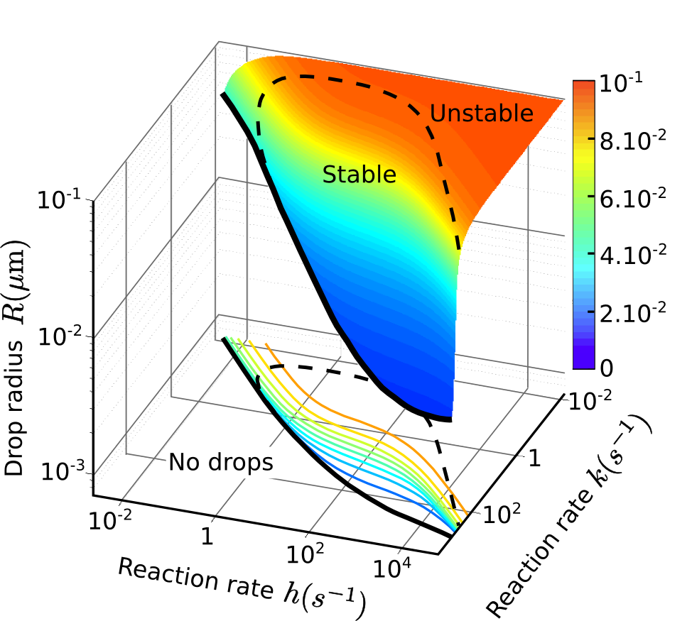
Figure S1: . The stability of a multi-drop system at fixed drop number density $\rho$. The steady-state radius $R^{*}$ (solution of $g_{0}(R^{*})=0$, Eq. (S75)) is controlled by the reaction rates $k$ and $h$. The continuous line delimits the region where $R^{*}$ exists. The steady-state is stable ($g_{1}(R^{*})<0$, Eq. (S81)) inside the region enclosed by the dashed line and the continuous line, and unstable ($g_{1}(R^{*})>0$) outside this region. Parameters: $\rho=1{\rm\mu m^{-3}},~{}\l_{c}=10^{-2}{\rm\mu m},~{}D=1{\rm\mu m^{2}s^{-1}},~{}\phi=5.10^{-4}{/\nu},~{}\hat{P}_{\rm in}=10^{-1}{/\nu},~{}\hat{P}_{\rm out}=10^{-4}{/\nu}$, where $\nu$ is the molecular volume of $P$ and $S$ and can be chosen arbitrarily.

III Equilibrium systems

When $k=0$ or/and $h=0$ no reactions occur in the steady-state and the system is in equilibrium conditions. From Eqs. (S6)-(S7), $k=0$ with $h>0$ leads to $P_{\rm tot}=\phi$, $S_{\rm tot}=0$, and $k>0$ with $h=0$ to $P_{\rm tot}=0$, $S_{\rm tot}=\phi$. When $k=h=0$ the ratio $\chi\equiv k/h$ and Eqs. (S6)-(S7) are undefined. We can nonetheless study such systems at concentrations $P_{\rm tot}$, $S_{\rm tot}$ using our non-equilibrium formalism by making $k$ and $h$ converge to zero while keeping $\chi$ in such a way that we recover the desired $P_{\rm tot},S_{\rm tot}$ from Eqs. (S6)-(S7):

$$\chi=\frac{\phi-P_{\rm tot}}{P_{\rm tot}}\ .$$ (S87)

Using this prescription we now calculate the steady-state drop radius $R^{*}$ and determine its stability. Taking $k,h$ to zero implies that $\xi\rightarrow\infty$ thus $x,y\rightarrow 0$ (but $y/x=R/L$) and therefore the steady-state condition Eq. (S75) becomes

$$(R^{*})^{3}=\frac{\lambda}{\lambda+1}L^{3}\ ,$$ (S88)

and using Eqs. (S87) and (S76) we find

$$(R^{*})^{3} = \frac{P_{\rm tot}-P_{\rm out}}{\hat{P}_{\rm in}}L^{3}\left(1+{\cal O}\left(\frac{\hat{P}_{\rm out}}{\hat{P}_{\rm in}}\right)\right)\ .$$ (S89)

Since at equilibrium there are no concentration gradients (this can be seen by taking $k=h=0$ in Eqs. (S1)-(S4)), this result can also be recovered simply by imposing the conservation of the number of molecules $P$ in the system: $R^{3}P_{\rm in}+(L^{3}-R^{3})P_{\rm out}=L^{3}P_{\rm tot}$. Plugging the Gibbs-Thomson relation (Eq. (S21)) in this result, we find the influence of the surface tension on the drop’s radius:

$$(R^{*})^{3}=\left(\frac{P_{\rm tot}-\hat{P}_{\rm out}}{\hat{P}_{\rm in}}-\frac{\hat{P}_{\rm out}l_{c}}{\hat{P}_{\rm in}R^{*}}\right)\left(1+{\cal O}\left(\frac{\hat{P}_{\rm out}}{\hat{P}_{\rm in}}\right)\right)L^{3}\ .$$ (S90)

The drop radius thus scales as the system size ($\propto L$) with a negative finite size correction ($\propto 1/R$). We also find the radius $R_{n}$ of the nucleus, which is the smallest drop that can exist:

$$R_{n}\simeq\frac{\hat{P}_{\rm out}l_{c}}{P_{\rm tot}-\hat{P}_{\rm out}}\ .$$ (S91)

Smaller drops dissolve because the concentration of $P$ outside the drop next to interface is larger than the total concentration $P_{\rm tot}$. We now study the stability of a multi-drop system by taking $k,h=0$ (leading to $x,y\rightarrow 0$ but $y/x=R/L$) in Eqs. (LABEL:eq:PRL:SI:f1):

$$f_{1} = 0$$ (S92)

$$f_{2} = 0$$ (S93)

$$f_{3} = 0$$ (S94)

$$f_{4} = -1+{\cal O}\left(\frac{R}{L}\right)\ ,$$ (S95)

and it follows that the stability relation (Eq. (S81)) is:

$$g_{1}\simeq\frac{4\pi D\hat{P}_{\rm out}l_{c}}{R^{*}}>0\ .$$ (S96)

Since $g_{1}>0$ for all radii $R^{*}$ we recover the equilibrium result that a multi-drop system is always unstable to Ostwald ripening Lifshitz and Slyozov (1961).

IV Non-equilibrium systems

We now focus on non-equilibrium systems ($k,h>0$). We first expose qualitative arguments showing that drops shrink when chemical reactions are present, then we study quantitatively multi-drop systems in different regimes based on the drop radius $R$ and the inter-drop distance $L$ compared to the gradient length scale $\xi$, and the reaction rates $k,h$.

IV.1 Chemical reactions lead do drop shrinkage and larger critical radius

We first consider an equilibrum ($k=h=0$) single-drop system with total concentrations $P_{\rm tot}$ and $S_{\rm tot}$ and $\phi\equiv P_{\rm tot}+S_{\rm tot}\ll 1$. The drop size is given by Eq. (S90). We then switch on the chemical reactions ($k,h>0$) in such a way that $P_{\rm tot}$ and $S_{\rm tot}$ remain unchanged ($k/h$ is given by Eq. (S87)). Outside the drop, the concentrations of both $P$ and $S$ are small and we neglect the chemical reactions. Inside the drop however, the $P$ concentration is high so we expect that the reaction $P\rightarrow^{k}S$ dominates and depletes $P$ from the drop, leading to the drop’s shrinkage. From this intuitive argument we expect that drops are smaller when chemical reactions are present compared to the equilibrium case.

We now show that this argument is indeed correct. At the exact time $t=0$ at which chemical reactions are switched on, the concentration profiles are flat inside and outside the drop and we can predict qualitatively how the system reacts after a small time interval $t=dt$. Using the reaction-diffusion equations (Eqs. (S1)-(S3)) with $\nabla^{2}P_{\rm in/out}=0$ we find the variation of the concentration $P$ inside and outside the drop:

$$\frac{dP_{\rm in}}{dt} = -k\hat{P}_{\rm in}+hS_{\rm tot}$$ (S97)

$$\frac{dP_{\rm out}}{dt} = -kP_{\rm out}+hS_{\rm tot}\ ,$$ (S98)

and since $S_{\rm tot}=P_{\rm tot}k/h$ (Eq. (S7)):

$$\frac{dP_{\rm in}}{dt} = -k\left(\hat{P}_{\rm in}-P_{\rm tot}\right)$$ (S99)

$$\frac{dP_{\rm out}}{dt} = k\left(P_{\rm tot}-P_{\rm out}\right)\ .$$ (S100)

$\hat{P}_{\rm in}>P_{\rm tot}>P_{\rm out}$ is a condition for phase separation to occur due to the conservation of the number of molecules $P$ in the system. Moreover we focus only on systems where the drop density $R^{3}/L^{3}$ is small, so from Eq. (S90) we must have $P_{\rm tot}\ll\hat{P}_{\rm in}$. As a result, the decrease in concentration inside the drop must be larger than the increase in concentration outside the drop. Because of the fixed interfacial boundary conditions, we expect the gradient inside the drop next to the interface to be greater than that right outside the drop, i.e.,

$$\left.\frac{\partial P_{\rm in}}{\partial r}\right|_{R}>\left.\frac{\partial P_{\rm out}}{\partial r}\right|_{R}\ .$$ (S101)

Therefore, the concentration of $P$ is depleted at the interface, and as a result the drop shrinks.

Let us now see the effect of chemical reactions on the critical radius, or nucleus radius (see Eq. (S91) for the equilibrium case). Consider a nucleus at equilibrium condition ($k=h=0$) with radius given by Eq. (S91). From the Gibbs-Thomson relation (Eq. (S21)) we know that the $P$ concentration right outside the nucleus is identical to $P_{\rm tot}$. When chemical reactions are turned on (keeping $P_{\rm tot},S_{\rm tot}$ constant) the nucleus must shrink from the argument we have just exposed, and as a result the concentration of $P$ just outside the nucleus will exceed $P_{\rm tot}$ (Eq. (S21)). This breaks the requirement that the total number of molecules $P$ must be conserved, thus leading to the nucleus dissolution. To compensate for this effect the nucleus in non-equilibrium conditions is necessarily larger than the nucleus at equilibrium.

We have shown qualitatively that when chemical reactions are turned on, drops shrink while the size of the smallest possible drop that can exist, the nucleus, is larger. The evaluation of the steady-state radius is more involved and must account for the chemical reactions-induced concentration gradients (Eqs. (S22)-(S25)) (see Sec. IV.2-IV.4).

IV.2 Large drops ($R\gg\xi$)

We focus here on the regime where drop radii $R$ are large compared to the gradient length scale $\xi$. Since the inter-drop distance $L$ is always larger than $R$ this regime also implies that $L\gg\xi$.

IV.2.1 Steady-state

We expand the steady-state condition Eq. (S75) for $x\gg y\gg 1$ and find:

$$y=\frac{1+\lambda}{1-\lambda}\left(1+{\cal O}\left(\frac{1}{x}\right)+{\cal O}\left(e^{-2(x-y)}\right)+{\cal O}\left(e^{-2y}\right)\right).$$ (S102)

For $y\gg 1$ to be true we must also have

$$\lambda<1,\quad{\cal O}(\lambda)={\cal O}(1)\ ,$$ (S103)

and we further expand using $\lambda-1$ as a small parameter:

$$y=\frac{2}{1-\lambda}\left(1+{\cal O}\left(\frac{1}{y}\right)+{\cal O}\left(e^{-2(x-y)}\right)\right)\ .$$ (S104)

Using Eqs. (S76) and expanding further in the small parameters $l_{c}/R^{*}$ and $\xi/R^{*}$ we get the steady-state radius $R^{*}$:

$$(R^{*})^{3} = \left(a+\frac{b}{R^{*}}\right)L^{3}\ ,$$ (S105)

with

$$a = \left(\frac{\phi-\hat{P}_{\rm out}}{\hat{P}_{\rm in}}-\frac{\chi}{2}\left(1+{\cal O}\left(\frac{1}{y}\right)\right)\right)\left(1+{\cal O}\left(\frac{\hat{P}_{\rm out}}{\hat{P}_{\rm in}}\right)\right)$$ (S106)

$$b = -\frac{\hat{P}_{\rm out}l_{c}}{\hat{P}_{\rm in}}\left(1+{\cal O}\left(\frac{\hat{P}_{\rm out}}{\hat{P}_{\rm in}}\right)\right)+\frac{\chi\xi}{2}\left(1+{\cal O}\left(\frac{1}{y}\right)+{\cal O}\left(e^{-2(x-y)}\right)\right)\ .$$ (S107)

In the large drop limit $b/R^{*}\rightarrow 0$ and there is a critical rate $k_{u}$ above which drops cease to exist ($R^{*}<0$):

$$k_{u}=\frac{2(\phi-\hat{P}_{\rm out})h}{\hat{P}_{\rm in}}\left[1+{\cal O}\left(\frac{\hat{P}_{\rm out}}{\hat{P}_{\rm in}}\right)\right]\ .$$ (S108)

We will later show that drops can still exist for $k>k_{u}$ but only with radii $R^{*}$ smaller than the gradient length scale $\xi$ ($y<1$). From Eq. (S105) we also see that $R^{*}$ scales as the system size $(\propto L)$, with a finite size correction ($b/R$). When $k=0$ and $h>0$ ($\chi=0$) no chemical reactions occur and we recover the equilibrium steady-state radius (Eq. (S90)) because $P_{\rm tot}=\phi$ (Eq. (S87)). In particular the finite size correction is negative ($b=-\hat{P}_{\rm out}l_{c}/\hat{P}_{\rm in}$) and originates from the Gibbs-Thomson relation (Eq. (S21)). Interestingly when chemical reactions are switched on ($k,h>0$) the correction becomes positive if the rate $k$ is larger than a critical value which we find by solving $b(k)=0$:

$$k=\frac{2l_{c}\hat{P}_{\rm out}h^{3/2}}{D^{1/2}\hat{P}_{\rm in}}\left[1+{\cal O}\left(\frac{k}{h}\right)+{\cal O}\left(\frac{\hat{P}_{\rm out}}{\hat{P}_{\rm in}}\right)+{\cal O}\left(\frac{1}{y}\right)+{\cal O}\left(e^{-2(x-y)}\right)\right]\ ,$$ (S109)

where we have used the fact that in the large drop regime $k$ must be smaller than $k_{u}$, therefore $k/h$ is always small. We shall see that this transition to an “inverse Gibbs-Thomson regime” indeed affects the system behaviour.

IV.2.2 Stability

We expand Eqs. (LABEL:eq:PRL:SI:f1) for $x\gg y\gg 1$:

$$f_{1} = -1+{\cal O}\left(ye^{-2(x-y)}\right)$$ (S110)

$$f_{2} = 1+{\cal O}\left(\frac{1}{x}\right)+{\cal O}\left(ye^{-2(x-y)}\right)$$ (S111)

$$f_{3} = -y\left(1+{\cal O}\left(\frac{1}{y}\right)\right)$$ (S112)

$$f_{4} = -y\left(1+{\cal O}\left(\frac{1}{y}\right)+{\cal O}\left(e^{-2(x-y)}\right)\right).$$ (S113)

From the definitions of $H_{\rm in/out}$ (Eqs. (S43),(S44)) we have

$$H_{\rm out}-H_{\rm in}=-\chi\hat{P}_{\rm in}\left(1+{\cal O}(\chi)+{\cal O}\left(\frac{\hat{P}_{\rm out}}{\hat{P}_{\rm in}}\right)\right)\ ,$$ (S114)

and by using the steady-state radius Eq. (S105) in the definitions of $H_{\rm in/out}$, we find

$${\cal O}\left(H_{\rm in}\right)={\cal O}\left(H_{\rm out}\right)={\cal O}\left(\hat{P}_{\rm in}\chi\right)\ .$$ (S115)

Therefore Eq. (S81) becomes

$$g_{1} = 4\pi D\left(-\chi\hat{P}_{\rm in}\left(1+\delta_{1}\right)+\frac{2l_{c}\hat{P}_{\rm out}}{\xi}(1+\delta_{2})\right)$$ (S116)

$$= 4\pi D\left(-\chi\hat{P}_{\rm in}\left(1+\delta_{1}\right)+\frac{2l_{c}\hat{P}_{\rm out}h^{1/2}}{D^{1/2}}\left(1+\delta_{2}\right)\right)\ ,$$ (S117)

with

$$\delta_{1} = {\cal O}(\chi)+{\cal O}\left(\frac{\hat{P}_{\rm out}}{\hat{P}_{\rm in}}\right)+{\cal O}\left(\frac{1}{x}\right)+{\cal O}\left(ye^{-2(x-y)}\right)$$ (S118)

$$\delta_{2} = {\cal O}(\chi)+{\cal O}\left(\frac{1}{y}\right)+{\cal O}\left(e^{-2(x-y)}\right)\ .$$ (S119)

Remembering that $\chi\equiv k/h$, we see that the system is unstable at small $k$ ($g_{1}>0$) and stable at large $k$ ($g_{1}<0$). We seek the critical rate $k_{l}$ at which the stability-instability transition occurs ($g_{1}(k_{l})=0$):

$$k_{l} = \frac{2l_{c}\hat{P}_{\rm out}h^{3/2}}{D^{1/2}\hat{P}_{\rm in}}\left(1+{\cal O}\left(\frac{k_{l}}{h}\right)+{\cal O}\left(\frac{\hat{P}_{\rm out}}{\hat{P}_{\rm in}}\right)+{\cal O}\left(\frac{1}{y}\right)+{\cal O}\left(ye^{-2(x-y)}\right)\right)\ .$$ (S120)

Interestingly the rate $k_{l}$ at which the system transition from the unstable to the stable regime is the same rate at which the system transition from the Gibbs-Thomson regime to the “inverse Gibbs-Thomson regime” (Eq. (S109).

If $k_{l}<k_{u}$ then ${\cal O}(k_{l}/h)$ is always small (Eq. (S108))). On the contrary when $k_{l}>k_{u}$, then ${\cal O}(k_{l}/h)>1$ and $k_{l}$ is not defined anymore since large drops dissolve for $k>k_{u}$. Therefore there exists a critical backward rate $h_{0}$ associated to this transition, which we will now discuss.

IV.2.3 Critical backward rate $h_{0}$

We have seen that large drops ($R^{*}>\xi$) can exist when the forward rate $k$ is smaller than the critical rate $k_{u}$ (Eq. (S108)) and are unstable to Ostwald ripening for $k<k_{l}$ and stable for $k>k_{l}$ (Eq. (S120)). When the backward rate $h$ is larger than a critical value $h_{0}$, the unstability-stability transition rate $k_{l}$ falls outside the region of existence of the large drop regime ($k_{l}>k_{u}$), and is therefore undefined. In this case large drops are always unstable. We find $h_{0}$ by solving $k_{l}(h_{0})=k_{u}(h_{0})$:

$$h_{0}=\frac{D}{l_{c}^{2}}\left(\frac{\phi-\hat{P}_{\rm out}}{\hat{P}_{\rm out}}\right)^{2}\left[1+{\cal O}\left(\frac{\phi-\hat{P}_{\rm out}}{\hat{P}_{\rm in}}\right)+{\cal O}\left(\frac{\hat{P}_{\rm out}}{\hat{P}_{\rm in}}\right)+{\cal O}\left(\frac{1}{y}\right)+{\cal O}\left(e^{-2(x-y)}\right)\right]\ .$$ (S121)

By expressing the gradient length scale $\xi$ for $h=h_{0}$ we find another interesting transition associated to $h_{0}$:

$$\xi(h_{0}) = \sqrt{\frac{D}{k+h_{0}}}$$ (S122)

$$= \sqrt{\frac{D}{h_{0}}}\left(1+{\cal O}\left(\frac{k}{h_{0}}\right)\right)$$ (S123)

$$\simeq \frac{\hat{P}_{\rm out}l_{c}}{\phi-\hat{P}_{\rm out}}$$ (S124)

$$= R_{n}\ ,$$ (S125)

where we used again the fact that $k/h$ is always small in the large drop regime since $k<k_{u}$ (Eq. (S108)) and where $R_{n}$ is the radius of the nucleus in equilibrium conditions (Eq. (S91)), since $P_{\rm tot}\simeq\phi$ for $k<k_{u}$ (eq (S6)). In other words, when $h>h_{0}$, the gradient length scale $\xi$ is smaller than the equilibrium nucleus $R_{n}$. Since in a non-equilibrium system the size of the nucleus is larger than in an equilibrium system (Sec. IV.1), the situation $h>h_{0}$ corresponds to the case where drops are always larger than $\xi$.

We have shown in the regime $k<k_{u}$ that when the backward rate is larger than the critical value $h_{0}$ drops are always larger than the gradient length scale $\xi$ and unstable to Ostwald ripening. We will later see that $h_{0}$ is also associated to a transition for small drops ($R<\xi$) in the $k>k_{u}$ regime.

IV.3 Small drops and low drop number density ($R\ll\xi$ and $L\gg\xi$)

We now consider the regime where the drop radii $R$ are small and the inter-drop distance $L$ is large, compared to the gradient length scale $\xi$.

IV.3.1 Steady-state

We expand for $x\gg 1$ and $y\ll 1$ the steady-state condition (Eq. (S75)):

$$\frac{y^{2}}{3}=\lambda\left(1+{\cal O}\left(\frac{1}{x}\right)+{\cal O}(y)\right)\ ,$$ (S126)

and $\lambda$ (Eq. (S76)):

$$\lambda=\frac{\phi-P_{\rm out}(1+\chi)}{\hat{P}_{\rm in}\chi}\left(1+{\cal O}\left(\frac{\phi-\hat{P}_{\rm out}}{\hat{P}_{\rm in}\chi}\right)+{\cal O}\left(\frac{\hat{P}_{\rm in}}{\frac{\phi}{1+\chi}-\hat{P}_{\rm out}}\frac{R}{L^{3}}\right)+{\cal O}\left(\frac{1}{\chi}\frac{R}{L^{3}}\right)\right)\ .$$ (S127)

From these two results we find an expression of the steady-state drop radius:

$$R_{u} = \sqrt{\frac{3D\left(\frac{\phi}{1+\chi}-\hat{P}_{\rm out}\left(1+\frac{l_{c}}{R}\right)\right)}{k\hat{P}_{\rm in}}}$$

$$\times\left(1+{\cal O}\left(\frac{1}{x}\right)+{\cal O}\left(y\right)+{\cal O}\left(\frac{\phi-\hat{P}_{\rm out}}{\hat{P}_{\rm in}\chi}\right)+{\cal O}\left(\frac{\hat{P}_{\rm in}}{\frac{\phi}{1+\chi}-\hat{P}_{\rm out}}\frac{R^{3}}{L^{3}}\right)+{\cal O}\left(\frac{1}{\chi}\frac{R^{3}}{L^{3}}\right)\right)\ ,$$

and if $R$ is much larger than the capillary length $l_{c}$ we have:

$$R_{u}\simeq\sqrt{\frac{3D\left(\frac{\phi}{1+\chi}-\hat{P}_{\rm out}\right)}{k\hat{P}_{\rm in}}}\ .$$ (S129)

We can now check self-consistently that the “${\cal O}(.)$” quantities here and in Eq. (S127) are indeed small. We start with the condition ${\cal O}(y)\ll 1$ by comparing $R_{u}$ to $\xi$ which provides a lower bound on the rate $k$ for this regime:

$$k \gg \frac{\phi-\hat{P}_{\rm out}}{\hat{P}_{\rm in}}h~{}\approx k_{u}\ .$$ (S130)

Note that $k_{u}$ is the upper bound on the rate $k$ for the large drop regime ($R\gg\xi$, Eq. (S108)). This together with the fact that $\hat{P}_{\rm in}>\phi>\hat{P}_{\rm out}$ must be true in a phase-separating system shows that ${\cal O}((\phi-\hat{P}_{\rm out})/\hat{P}_{\rm in}\chi)$ is small. ${\cal O}(1/x)$, ${\cal O}[\hat{P}_{\rm in}/(\phi/(1+\chi)-\hat{P}_{\rm out})R^{3}/L^{3}]$ and ${\cal O}[R^{3}/(\chi L^{3})]$ can be set arbitrary small by increasing $L$, or equivalently by decreasing the drop number density $\rho$.

IV.3.2 Critical forward rate $k_{c}$

When the forward rate $k$ increases the steady-state drop radius $R_{u}$ decreases and falls to zero for large enough $k$. The critical rate $k_{c}$ at which this transition occurs can be estimated by solving $R_{u}(k_{c})=0$ (Eq. (IV.3.1)).

$$R_{u} = 0$$ (S131)

$$\Rightarrow\ \ aR^{3}+bR^{2}+cR+d = 0\ ,$$ (S132)

with

$$a = \frac{k_{c}\hat{P}_{\rm in}}{3D}$$ (S133)

$$b = 0$$ (S134)

$$c = -\left(\frac{\phi}{1+\frac{k_{c}}{h}}-\hat{P}_{\rm out}\right)$$ (S135)

$$d = \hat{P}_{\rm out}l_{c}\ .$$ (S136)

This is a cubic equation in $R$ and according to the signs of the coefficients $a,b,c,d$ there are either two real positive solutions if the determinant $\Delta=18abcd-4b^{3}d+b^{2}c^{2}-4ac^{3}-27a^{2}d^{2}$ is positive, and no real positive solutions if $\Delta<0$. We ignore complex or negative solutions since they are unphysical. The expression of $\Delta$ is:

$$\Delta=\frac{k\hat{P}_{\rm in}}{D}\left[\frac{4}{3}\left(\frac{\phi}{1+\frac{k}{h}}-\hat{P}_{\rm out}\right)^{3}-\frac{3k\hat{P}_{\rm in}\hat{P}_{\rm out}^{2}l_{c}^{2}}{D}\right]\ .$$ (S137)

At small rate $k$ the discriminant $\Delta$ is positive so two steady-state radii $R$ exist, the larger radius being $R_{u}$. At large $k$ the discriminant $\Delta$ becomes negative so there are no steady-state radii and therefore no drops can exist in the system. The critical rate $k_{c}$ at which this transition occurs is solution of $\Delta(k_{c})=0$:

$$\frac{k_{c}}{\left(\frac{\phi}{1+\frac{k_{c}}{h}}-\hat{P}_{\rm out}\right)^{3}}=\frac{4}{9}\frac{D}{l_{c}^{2}}\frac{1}{\hat{P}_{\rm in}\hat{P}_{\rm out}^{2}}\ .$$ (S138)

We can find upper bounds on $k_{c}$ by noticing the two following elements: first, this equation admits a solution only if $\phi/(1+k_{c}/h)-\hat{P}_{\rm out}>0$, and second, $k_{c}$ is a monotonic and increasing function of $h$ therefore $k_{c}$ is upper bounded by $k_{c}(h\rightarrow\infty)$. The critical rate $k_{c}$ is thus bounded as follow:

$$k_{c}<{\rm min}\left[\frac{\phi-\hat{P}_{\rm out}}{\hat{P}_{\rm out}}h\ \ \ ,\ \ \ \frac{4}{9}\frac{D}{l_{c}^{2}}\frac{\left(\phi-\hat{P}_{\rm out}\right)^{3}}{\hat{P}_{\rm in}\hat{P}_{\rm out}^{2}}\right]\ .$$ (S139)

In the case where $h>h_{0}$ (Eq. (S121)) the critical rate $k_{c}$ becomes smaller than $k_{u}$. Since $k_{c}$ is only defined for small drops ($R\ll\xi$) and since only large drops exist for $k<k_{u}$ and $h>h_{0}$ (Sec. IV.2.3), then $k_{c}$ is not defined anymore in this case and drops dissolve only when $k>k_{u}$.

Note that we used the fact that $R\ll\xi$ in this regime to derive $k_{c}$. However this approximation becomes less accurate when $h$ is close to $h_{0}$ since the size of all drops becomes comparable to or larger than the gradient length scale $\xi$ (Sec. IV.2.3). Therefore when $h\approx h_{0}$ the critical rate $k_{c}$ as expressed in Eqs. (S138) and (S139) is only a rough approximation.

IV.4 Small drops and high drop number density ($R\ll\xi$ and $L\ll\xi$) in the $k\gg k_{u}$ regime

We now study the regime where the drop radii $R$ and the inter-drop distance $L$ are both small compared to the gradient length scale $\xi$, and we moreover focus only on the $k\gg k_{u}$ regime (Eq. (S108)).

IV.4.1 Steady-state

Expanding for $y\ll x\ll 1$, the steady-state condition Eq. (S75) becomes

$$x^{3}=\frac{(\lambda+1)y^{3}}{\lambda-\frac{y^{2}}{3}}\left(1+{\cal O}\left(x^{2}\right)\right)\ .$$ (S140)

Imposing $y\ll x\ll 1$ on this result leads to the following requirements:

$$\frac{y^{2}}{3}\ll\lambda\ll 1$$ (S141)

$$\Rightarrow {\cal O}\left(\frac{y^{3}}{x^{3}}\right)={\cal O}(\lambda)$$ (S142)

$$\Rightarrow x^{3}\ll y\ ,$$ (S143)

and Eq. (S140) thus becomes:

$$x^{3}=\frac{y^{3}}{\lambda}\left(1+{\cal O}(x^{2})+{\cal O}\left(\frac{x^{3}}{y}\right)\right)\ .$$ (S144)

Plugging Eq. (S76) in this result we find the drop steady-state drop radius $R$:

$$R^{3} = \frac{\frac{\phi}{1+\chi}-\hat{P}_{\rm out}}{\hat{P}_{\rm in}}L^{3}\left[1+\frac{\chi}{1+\chi}\left({\cal O}\left(x^{2}\right)+{\cal O}\left(\frac{x^{3}}{y}\right)+{\cal O}\left(\frac{R^{3}}{L^{3}\chi}\right)+{\cal O}\left(\frac{\phi-\hat{P}_{\rm out}}{\hat{P}_{\rm in}\chi}\right)\right)\right.$$ (S145)

$$\left.+{\cal O}\left(\frac{1}{1+\chi}\frac{\hat{P}_{\rm out}}{\hat{P}_{\rm in}}\right)\right]\ .$$

We now determine that the terms “${\cal O}(.)$” are indeed small. $\hat{P}_{\rm in}>\phi>\hat{P}_{\rm out}$ must be true in a phase-separating system, and taking $k\gg k_{u}$ (Eq. (S108)) shows that ${\cal O}[(\phi-\hat{P}_{\rm out})/\hat{P}_{\rm in}\chi]$ and ${\cal O}[1/(1+\chi)\hat{P}_{\rm out}/\hat{P}_{\rm in}]$ are small. Using Eq. (S145) the condition ${\cal O}(R^{3}/(L^{3}\chi))\ll 1$ becomes:

$$\chi+\chi^{2}-\frac{\phi-\hat{P}_{\rm out}}{\hat{P}_{\rm in}} \gg 0$$ (S146)

$$\chi \gg \frac{1}{2}\left(\sqrt{1+4\frac{\phi-\hat{P}_{\rm out}}{\hat{P}_{\rm in}}}-1\right)\simeq\frac{\phi-\hat{P}_{\rm out}}{\hat{P}_{\rm in}}$$ (S147)

$$k \gg k_{u}\ ,$$ (S148)

which is a condition we have already imposed. Finally by using again Eq. (S145) the condition ${\cal O}(x^{3}/y)\ll 1$ leads to a lower bound on the drop number density $\rho$:

$$\rho\gg\frac{3}{4\pi}\left(\frac{k+h}{D}\right)^{3/2}\left(\frac{\hat{P}_{\rm in}}{\frac{\phi h}{k+h}-\hat{P}_{\rm out}}\right)^{1/2}\ .$$ (S149)

IV.4.2 Stability

Expanding for $y\ll x\ll 1$ and keeping in mind that $x^{3}\ll y$ (Eq. (S143)), Eqs. (LABEL:eq:PRL:SI:f1) become

$$f_{1} = -\frac{y^{2}}{3}\left(1+{\cal O}\left(y^{2}\right)\right)$$ (S150)

$$f_{2} = \frac{x^{3}}{3y}\left(1+{\cal O}(x)+{\cal O}\left(\frac{y}{x}\right)+{\cal O}\left(\frac{x^{3}}{y}\right)\right)$$ (S151)

$$f_{3} = -\frac{y^{2}}{3}\left(1+{\cal O}\left(y^{2}\right)\right)$$ (S152)

$$f_{4} = -1+{\cal O}(x)+{\cal O}\left(\frac{y}{x}\right).$$ (S153)

and using these results together with the steady-state condition Eq. (S144), Eq. (S81) becomes

$$g_{1}=4\pi D \left[-\frac{2y^{2}H_{\rm in}}{3}\left(1+{\cal O}(x)+{\cal O}\left(\frac{y}{x}\right)+{\cal O}\left(\frac{x^{3}}{y}\right)\right)+\frac{\hat{P}_{\rm out}l_{c}}{R}\left(1+{\cal O}(x)+{\cal O}\left(\frac{y}{x}\right)\right)\right].$$ (S154)

The system is unstable for small radii ($g_{1}>0$) and stable for large radii ($g_{1}<0$). The stability-instability boundary radius $R_{l}$ is the solution of $g_{1}(R_{l})=0$:

$$R_{l}y^{2}\simeq\frac{3\hat{P}_{\rm out}l_{c}}{2H_{\rm in}}\ .$$ (S155)

Expanding $H_{\rm in}$ gives

$$H_{\rm in}=\frac{\chi\hat{P}_{\rm in}}{1+\chi}\left(1+{\cal O}\left(\frac{\phi-\hat{P}_{\rm out}}{\chi\hat{P}_{\rm in}}\right)+{\cal O}\left(\frac{R^{3}}{L^{3}\chi}\right)\right)\ .$$ (S156)

and therefore we find:

$$R_{l}\simeq\left(\frac{3Dl_{c}\hat{P}_{\rm out}}{2k\hat{P}_{\rm in}}\right)^{\frac{1}{3}}\ .$$ (S157)

We check self-consistently the condition ${\cal O}(y)\ll 1$:

$$R_{l} \ll \xi$$ (S158)

$$\frac{D^{2}l_{c}^{2}\hat{P}_{\rm out}^{2}}{k^{2}\hat{P}_{\rm in}^{2}} \ll \frac{D^{3}}{h^{3}(1+\chi)^{3}}$$ (S159)

$$k \gg \frac{l_{c}\hat{P}_{\rm out}h^{3/2}}{D^{1/2}\hat{P}_{\rm in}}\left(1+{\cal O}\left(\frac{l_{c}\hat{P}_{\rm out}h^{1/2}}{D^{1/2}\hat{P}_{\rm in}}\right)\right)\simeq k_{l}\ .$$ (S160)

When $h<h_{0}$ we have $k_{l}<k_{u}$ by definition (Sec. IV.2.3) and therefore the above condition is always true in the $k\gg k_{u}$ regime that we are considering in this section. Using the expression of $h_{0}$ (Eq. (S121)) we also see that ${\cal O}(l_{c}\hat{P}_{\rm out}h^{1/2}/(D^{1/2}\hat{P}_{\rm in}))$ is always small when $h<h_{0}$. If on the contrary $h>h_{0}$ we have already seen that only large drops exist so $R_{l}$ is undefined.

IV.5 Stability diagrams

We have seen that in a multi-drop system chemical reactions control drop size and coarsening, and that different regimes exist depending on the reaction rates $k$ and $h$. In Fig. 3 (main text) we explicit these regimes by varying the rate $k$ while $h$ is fixed. For a different choice of $h$ the system can exhibit different features as shown in Fig. S2.

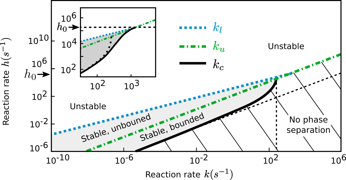
Figure S2: Stability diagram of a multi-drop system in the reaction rate space. In a multi-drop system, drop existence, radius and stability, depend on the chemical reaction rates $k$ and $h$. For backward rates $h$ smaller than $h_{0}$ (black arrow, (Eq. (S121))), multi-drop systems are stable against Ostwald ripening (grey region) if the forward rate $k$ is between $k_{l}$ (blue dotted line, Eq. (S120)) and $k_{c}$ (black continuous curve, Eq. (S138)). The upper bounds of $k_{c}$ estimated in Eq. (S139) are shown by the black dashed lines. In the white region, multi-drop systems are unstable and coarsen via Ostwald ripening. In the stable region (grey area), the drop radius is upper-bounded if $k>k_{u}$ (green irregular dashed line, Eq. (S108)), or unbounded otherwise. Phase separation is destroyed and drops dissolve in the hashed area. The validity of the expression of $k_{c}$ given by Eq. (S138) breaks down when the drop radius $R$ approaches the gradient length-scale $\xi$. In this region, we determined $k_{c}$ by solving exactly the steady-state relation Eq. (S75) (continuous black line in the insert figure. For comparison, $k_{c}$ determined from Eq. (S138) is showed by the dotted black line). Parameters: $l_{c}=10^{-2}{\rm\mu m},~{}D=1{\rm\mu m^{2}s^{-1}},~{}\phi=5.10^{-4}{/\nu},~{}\hat{P}_{\rm in}=10^{-1}{/\nu},~{}\hat{P}_{\rm out}=10^{-4}{/\nu}$, where $\nu$ is the molecular volume of $P$ and $S$ and can be chosen arbitrarily.

Part III Two dimensions

In two dimension space ($d=2$) the steady-state condition ($g_{0}(R^{*})=0$, Eq. (S38)) becomes

$$H_{\rm out}\left[AJ_{1}(\iota y^{*})-BY_{1}(-\iota y^{*})\right]-H_{\rm in}\frac{J_{1}(\iota y^{*})}{J_{0}(\iota y^{*})}=0$$ (S161)

with $y^{*}\equiv R^{*}/\xi$, and the linearised drop growth rate of drop 1 upon perturbing the steady-state $R_{1}\mapsto R^{*}+\epsilon$, $R_{2}\mapsto R^{*}-\epsilon$ with $\epsilon\ll R^{*}$ is

$$\frac{g_{1}(R^{*})}{4\pi DR^{*2}} = \mathcal{H}_{\rm out}\frac{\iota}{\xi}\left[-AJ_{1}(\iota y^{*})+BY_{1}(-\iota y^{*})\right]+H_{\rm out}\frac{\iota}{\xi}\left[-\mathcal{A}J_{1}(\iota y^{*})+\mathcal{B}Y_{1}(-\iota y^{*})\right]$$

$$+H_{\rm out}\frac{1}{\xi^{2}}\left[A\left(J_{0}(\iota y^{*})+\frac{\iota}{y^{*}}J_{1}(\iota y^{*})\right)+B\left(Y_{0}(-\iota y^{*})-\frac{\iota}{y^{*}}Y_{1}(-\iota y^{*})\right)\right]$$

$$+\mathcal{H}_{\rm in}\frac{\iota}{\xi}\frac{J_{1}(\iota y^{*})}{J_{0}(\iota y^{*})}-H_{\rm in}\frac{1}{\xi^{2}}\left[\frac{J_{0}(\iota y^{*})+\frac{\iota}{y^{*}}J_{1}(\iota y^{*})}{J_{0}(\iota y^{*})}+\left(\frac{J_{1}(\iota y^{*})}{J_{0}(\iota y^{*})}\right)^{2}\right]$$

with $x\equiv L/\xi$ and

$$A = \frac{Y_{1}(-\iota x)}{J_{1}(\iota x)Y_{0}(-\iota y^{*})+Y_{1}(-\iota x)J_{0}(\iota y^{*})}$$ (S163)

$$B = \frac{Y_{1}(\iota x)}{J_{1}(\iota x)Y_{0}(-\iota y^{*})+Y_{1}(-\iota x)J_{0}(\iota y^{*})}$$ (S164)

$$\mathcal{A} = \frac{\iota J_{1}(\iota x)Y_{1}(-\iota y^{*})Y_{0}(-\iota x)-\iota J_{1}(\iota y^{*})Y_{1}(-\iota x)Y_{0}(-\iota x)-\xi\frac{\mathcal{H}_{\rm out}}{H_{\rm out}}\left[J_{0}(\iota x)Y_{1}(-\iota x)Y_{0}(-\iota y^{*})+J_{1}(\iota x)Y_{0}(-\iota x)Y_{0}(-\iota y^{*})\right]}{\xi\left[J_{0}(\iota x)Y_{0}(-\iota y^{*})-Y_{0}(-\iota x)J_{0}(\iota y^{*})\right]\left[J_{1}(\iota x)Y_{0}(-\iota y^{*})+Y_{1}(-\iota x)J_{0}(\iota y^{*})\right]}$$

$$\mathcal{B} = \frac{-\iota J_{1}(\iota x)Y_{1}(-\iota y^{*})J_{0}(\iota x)+\iota J_{1}(\iota y^{*})Y_{1}(-\iota x)J_{0}(\iota x)+\xi\frac{\mathcal{H}_{\rm out}}{H_{\rm out}}\left[J_{0}(\iota x)Y_{1}(-\iota x)J_{0}(\iota y^{*})+J_{1}(\iota x)Y_{0}(-\iota x)J_{0}(\iota y^{*})\right]}{\xi\left[J_{0}(\iota x)Y_{0}(-\iota y^{*})-Y_{0}(-\iota x)J_{0}(\iota y^{*})\right]\left[J_{1}(\iota x)Y_{0}(-\iota y^{*})+Y_{1}(-\iota x)J_{0}(\iota y^{*})\right]}$$

$$H_{\rm in} = \hat{P}_{\rm in}-\frac{\Delta S\phi+\left(\hat{P}_{\rm in}-\Delta SP_{\rm out}(R^{*})\right)\left(1-\left(\frac{R^{*}}{L}\right)^{2}\right)}{(\chi+1)\left(1-(1-\Delta S)\left(\frac{R^{*}}{L}\right)^{2}\right)}$$ (S167)

$$H_{\rm out} = P_{\rm out}-\frac{\phi-\left(\hat{P}_{\rm in}-\Delta SP_{\rm out}(R^{*})\right)\left(\frac{R^{*}}{L}\right)^{2}}{(\chi+1)\left(1-(1-\Delta S)\left(\frac{R^{*}}{L}\right)^{2}\right)}.$$ (S168)

Note that we are interested only in the real parts of Eqs. (S161) and (III).

Part IV Simulation Methods

I General method

We study the dynamics of chemically active drops in a ternary fluid using Monte-Carlo simulation methods. We consider a ternary mixture $P,S,C$ on a two-dimensional square lattice where each site has the dimension $\Delta d$. Each particle $P$ interacts with its $8$ nearest neighbours so that every $P-P$ pair contributes to the system energy by $e_{AA}$. The total system Hamiltonian is

$$H=N_{PP}e_{PP}$$ (S169)

where $N_{PP}$ is the total number of $P-P$ pairs in the system. We enumerate the simulation steps carried out within a simulation time unit $\Delta t$. To simulate the system, we use the Metropolis-Hastings algorithm together with the Kawasaki exchange scheme kawasaki1972phase . The entire lattice is searched sequentially for sites occupied by a $P$ or $S$. When such site is found, one of its $8$ nearest neighbour is randomly selected. The two sites are then exchanged with the probability

$$p=\left\{\begin{array}[]{ll}e^{-\Delta H/(k_{b}T)}&\Delta H>0\\ 1&\Delta H\leq 0\end{array}\right.$$ (S172)

where $\Delta H$ is the change in Hamiltonian caused by the exchange, $T$ the temperature and $k_{b}$ the Boltzmann constant. We then consider the chemical reactions that convert $P$ into $S$ and vice versa:

$$\ce{$P$<=>[k][h]$S$}.$$ (S173)

where $k$ and $h$ are the reaction rate constants. The entire lattice is again sequentially searched for sites occupied by a $P$ or $S$. When a site with a $P$ is found, the $P$ is destroyed and replaced by a newly created $S$, with the probability $k$. If a site with a $S$ is found, the $S$ is destroyed and replaced with a newly created $P$, with the probability $h$.

II Equilibrium parameters: capillary length $l_{c}$ and dilute phase composition $\hat{P}_{\rm out}$

To determine the equilibrium ($k=h=0$) parameters $l_{c}$ and $\hat{P}_{\rm out}$ associated to our simulations, we simulate single-drop systems of different sizes and extract their drop radius $R$ and $P$ concentration $P_{\rm out}(R)$ in the dilute phase, and fit these results to the Gibbs-Thomson relation (Eq. (S21)) (Fig. S3).

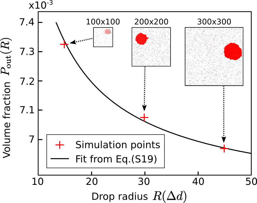
Figure S3: Determination of the equilibrium ($k=h=0$) parameters $l_{c}$ and $\hat{P}_{\rm out}$ associated to our simulations. We simulate three single-drop systems of different sizes (snapshots), extract their drop radius $R$ and concentration of $P$ in the diluted phase ($P_{\rm out}(R)$), and fit the results (red points) to the Gibbs-Thomson relation (Eq. (S21)). We perform a linear regression of $P_{\rm out}(R)\times R=\hat{P}_{\rm in}\times R+l_{c}$ and find $l_{c}=1.2\pm 0.1~{}\Delta d$ and $\hat{P}_{\rm out}=(6.79\pm 0.02).10^{-3}$ (see black curve for best fit). To cancel out fluctuations in $R$ and $P_{\rm out}(R)$ we calculate their mean values by averaging a large number of samples. Moreover $P_{\rm out}(R)$ is also spatially averaged in a square region in the dilute phase. Parameters: $P_{\rm tot}=1/13$, $S_{\rm tot}=3/130$, $e_{PP}=-9/7$, system sizes = $100\times 100$, $200\times 200$, $300\times 300$ $(\Delta d)^{2}$.

III Non-equilibrium concentration profiles

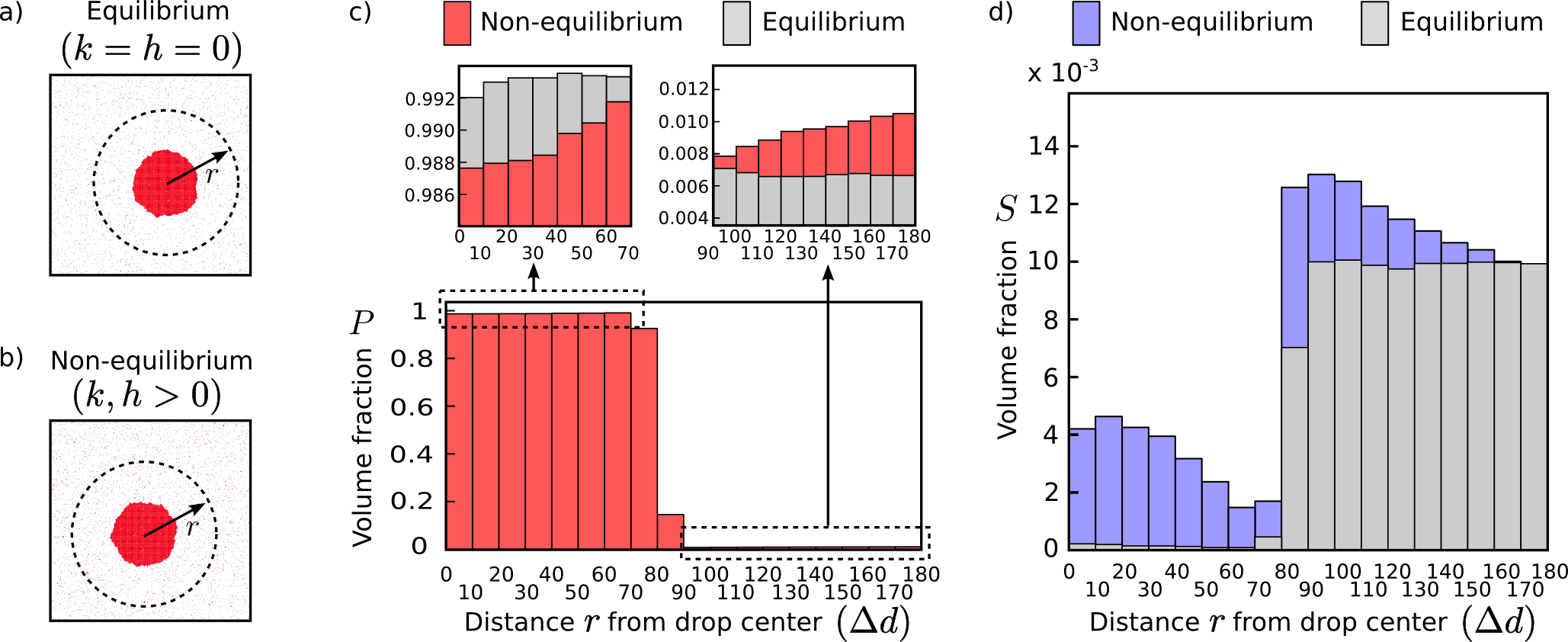
Figure S4: Volume fraction profiles in a single-drop system for equilibrium ($k=h=0$) (a)) and non-equilibrium ($k,h>0$) conditions (b)). c) At the drop interface, the $P$ profiles are similar both at equilibrium and non-equilibrium conditions. At non-equilibrium conditions, concentration gradients in $P$ and $S$ exist inside and outside drops (c) and d)). The profiles are radially averaged inside a disc centred on the drop center of mass (dashed line in a) and b)), then averaged over multiple samples. Parameters: system size=$500{\rm X}500~{}(\Delta d)^{2}$, disc radius=$180\Delta d$, $\phi=0.1$. $\epsilon_{PP}=-9/7$. Equilibrium parameters: $P_{\rm tot}=1/11$, $S_{\rm tot}=1/110$. Non-equilibrium parameters: $k=2\times 10^{-6}(\Delta t)^{-1}$, $h=2\times 10^{-5}(\Delta t)^{-1}$.

Our analytical work is based on the assumptions that the system is close to equilibrium and that local thermal equilibrium remains valid. The subsequent concentration profiles Eqs. (S22)-(S23) obey the equilibrium conditions at the drop’s interfaces (Eqs. (S20),(S21)) and contain spatial gradients inside and outside drops. Seeking for validation of these assumptions we study the concentration profiles in a single-drop system for equilibrium conditions ($k=h=0$) and non-equilibrium conditions ($k,h>0$) (Fig. S4). We obtain confirmation that the coexistence concentration of $P$ at the interface are similar at equilibrium and non-equilibrium, and that the profiles of $P$ and $S$ contain spatial gradients inside and outside the drop at non-equilibrium conditions.

IV Stability-instability boundary radius

We seek the stability-instability boundary radius (dashed line in Fig. 3 and Eq. (15), main text). At time $0$ we randomly distribute $P$ and $S$ molecules on the lattice in such a way that the system is inside the phase boundary ($P_{\rm tot}>\hat{P}_{\rm out}$, Fig. 1, main text) and globally at chemical equilibrium ($P_{\rm tot}=h\phi/(k+h)$, $S_{\rm tot}=k\phi/(k+h)$). In the early stage drops nucleate and grow, then drops undergo coarsening via coalescence and Ostwald ripening leading to an increase of the average drop radius. Eventually coarsening is arrested and the system reaches a steady-state composed of drops with similar radii. This particular steady-state radius, that is reached by starting from small drops, is defined as the stability-instability boundary radius. The coarsening and steady-state regimes are shown in Fig. S5.

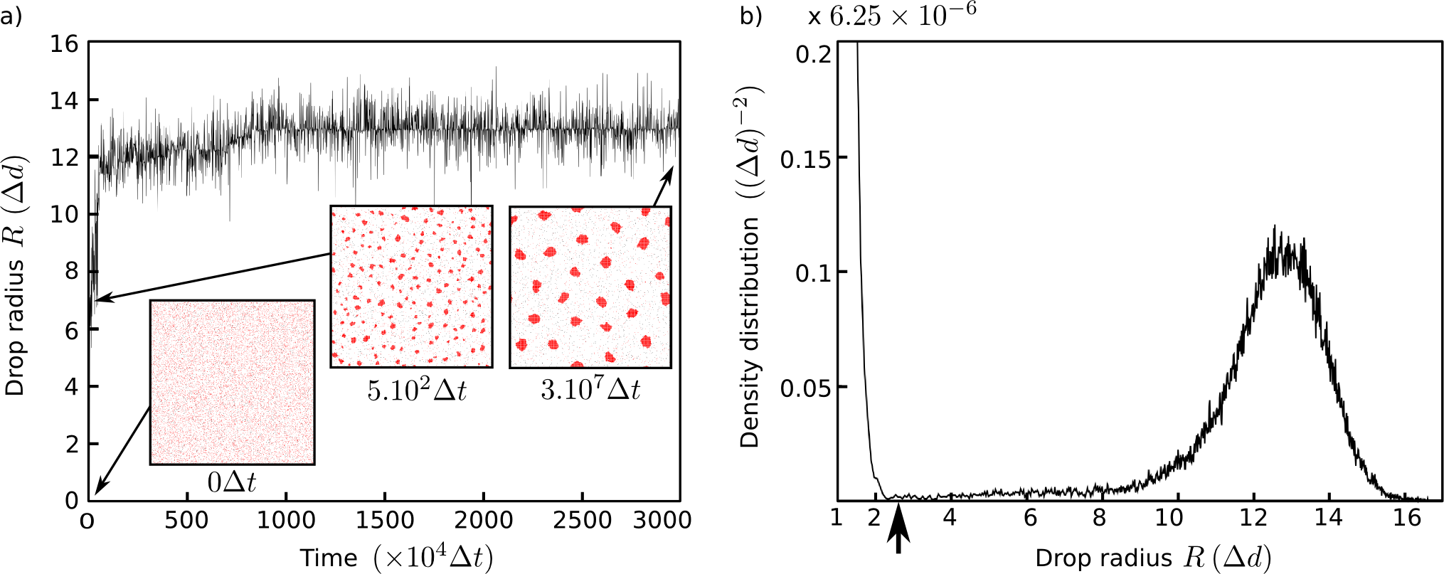
Figure S5: Determination of the stability-instability boundary radius. At $\Delta t=0$ particles $P$ and $S$ are randomly distributed on the lattice, ensuring global chemical equilibrium ($P_{\rm tot}=h\phi/(k+h)$, $S_{\rm tot}=k\phi/(k+h)$). a) In the early stage drops nucleate and grow, then drops undergo coarsening via coalescence and Ostwald ripening leading to an increase of the average drop radius. Eventually coarsening is arrested and the system reaches a steady-state composed of drops with similar radii. This particular steady-state radius, that is reached when starting with small drops, is defined as the stability-instability boundary radius. Snapshots (inserts) are taken at different times and $P$ and $S$ particles and shown with red dots and blue dots, respectively. b) The steady-state radius is defined by the location of the highest peak in the drop radius distribution. The radius distribution is averaged during the second half of the simulation. We neglect the small drops that form transiently due to the stochastic fluctuations of the concentrations by ignoring drops that contain less than $20$ $P$ molecules (arrow). Parameters: system size= $400\times 400~{}(\Delta d)^{2}$, $\phi=0.1$, $e_{PP}=-9/7$, $h=10^{-4}(\Delta t)^{-1}$, $k=10^{-5}(\Delta t)^{-1}$.

V Comparison between theoretical results and simulations

We now compare our simulations to our theoretical predictions for 2D systems (Part III). Specifically we analyse the stability-instability boundary radius. We first establish the correspondence between the time and length units in the simulation ($\Delta t$, $\Delta d$) and the physical units (seconds, meters). The diffusion coefficient associated to a random walk on our lattice is given by

$$D=\frac{(\Delta d)^{2}}{2\Delta t}.$$ (S174)

Equating $D$ to the typical protein diffusion coefficient in the cytoplasm, $1{\rm\mu m^{2}.s^{-1}}$, and $\Delta d$ to the typical protein size, $10\rm nm$, we express the physical time and length in terms of $\Delta t$ and $\Delta d$

$$1{\rm s} = 2.10^{4}\Delta t$$ (S175)

$$1{\rm\mu m} = 10^{2}\Delta d.$$ (S176)

Using this correspondence the parameters $l_{c}$ and $\hat{P}_{\rm out}$ (see Fig. S3) become

$$l_{c} = 1.2\times 10^{-2}\rm\mu m$$ (S177)

$$\hat{P}_{\rm out} = 7.79\times 10^{-3}\quad$$ (S178)

Analysing the concentration profiles at the interface (Fig. S4) we approximate

$$\hat{P}_{\rm in} = 1$$ (S180)

$$\Delta S = 0.1$$ (S181)

Using these parameters in our theoretical predictions for 2D systems (see Part III) we determine the steady-state radius $R^{*}$ (see Eq. (S161)) and their stability (see Eq. (III)) as functions of the rate $k$ and for fixed rate $h$. We show the phase stability diagram in Fig. S6, where the dashed line represents the stability-instability boundary radius. We compare this boundary to our simulation results (red points in Fig. S6) and find a good agreement between theory and simulations. Note that we studied the regions close to the critical rates $k_{c}$ (Fig. S6(a)) and $k_{l}$ Fig. S6(b)) with two different choices of $h$ in order to avoid excessively large simulation times.

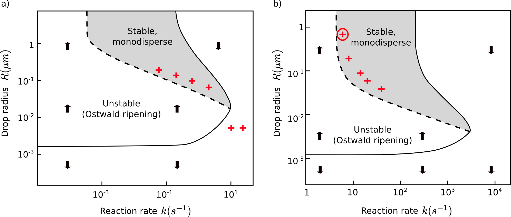
Figure S6: Comparison between 2D theoretical predictions and numerical simulations. The rate $k$ is varied keeping the rate $h$ fixed. A steady-state drop radius $R^{*}$ (solution of $g_{0}(R^{*})=0$, Eq. (S161)) exists in the region enclosed by the continuous line. Outside this region no steady-states exist and drops dissolve (downward arrows). The steady-state $R^{*}$ is stable inside the grey region ($g_{1}(R^{*})<0$, Eq. (III)). Outside the grey region the steady-state is unstable to Ostwald ripening ($g_{1}(R^{*})>0$) causing the average drop radius to increase (upward arrows). The stability-instability boundary ($g_{1}(R^{*})=0$) is shown with a dashed line. Regarding the simulations, the lattice is initialized at $\Delta t=0$ by randomly distributing $P$ and $S$ on the lattice in such a way that the system is inside the phase boundary ($P_{\rm tot}>\hat{P}_{\rm out}$, and see Fig. 1 in main text) and globally at chemical equilibrium ($P_{\rm tot}=h\phi/(k+h)$, $S_{\rm tot}=k\phi/(k+h)$). In the early stage drops nucleate, grow and coarsen, leading to an increase of the mean drop radius, then coarsening is stopped and the system reaches a steady-state defined as the stability-instability boundary (Fig. S5). Simulation data are shown in red. The two rightmost crosses in a) represent the size of the lattice site ($\sim 10^{-2}\rm{\mu m}$), i.e., there are no drops in system. The encircled cross in b) indicates that the system coarsened until a single drop remained even in the largest system simulated. There is a good agreement between theory and simulations. The duration of simulations range from $1.8\times 10^{7}\Delta t$ to $2\times 10^{8}\Delta t$. Parameters: $\phi=0.1$, $D=1\rm{\mu m^{2}s^{-1}}$, $\hat{P}_{\rm in}=1$, $\hat{P}_{\rm out}=7.79\times 10^{-3}$, $\Delta S=0.1$, $l_{c}=1.2\times 10^{-2}\rm{\mu m}$, $e_{PP}=-9/7$. Figure a): system size=$400X400~{}({\rm\Delta d})^{2}$, $h=2~{}s^{-1}$. Figure b): system size=$300\times 300~{}({\rm\Delta d})^{2}$ to $400\times 400~{}({\rm\Delta d})^{2}$, $h=2\times 10^{3}~{}s^{-1}$. See Sec. V for the equivalence between simulation and physical units.

References

Bray (2002)
A. J. Bray,
Advances in Physics 51,
481 (2002).
Brangwynne (2011)
C. Brangwynne,
Soft Matter 7,
3052 (2011).
Hyman et al. (2014)
A. A. Hyman,
C. A. Weber, and
F. Jülicher,
Annual Review of Cell and Developmental Biology
30, 39 (2014).
Anderson et al. (2009)
P. Anderson,
N. Kedersha,
V. Kim,
I. Ryu, and
S. Jang,
Current biology 19,
R397 (2009).
Protter and Parker (2016)
D. S. Protter and
R. Parker,
Trends in Cell Biology 26,
668 (2016).
Zwicker et al. (2014)
D. Zwicker,
M. Decker,
S. Jaensch,
A. A. Hyman, and
F. Jülicher,
Proceedings of the National Academy of Sciences
111, E2636
(2014).
Brangwynne et al. (2009)
C. Brangwynne,
C. Eckmann,
D. Courson,
A. Rybarska,
C. Hoege,
J. Gharakhani,
F. Jülicher,
and A. Hyman,
Science 324,
1729 (2009).
Voronina et al. (2011)
E. Voronina,
G. Seydoux,
P. Sassone-Corsi,
and I. Nagamori,
Cold Spring Harbor Perspectives in Biology
3, a002774
(2011).
Lee et al. (2013)
C. F. Lee,
C. P. Brangwynne,
J. Gharakhani,
A. A. Hyman, and
F. Jülicher,
Physical Review Letters 111,
088101 (2013).
Saha et al. (2016)
S. Saha,
C. A. Weber,
M. Nousch,
O. Adame-Arana,
C. Hoege,
M. Y. Hein,
E. Osborne-Nishimura,
J. Mahamid,
M. Jahnel,
L. Jawerth,
et al., Cell 166,
1572 (2016).
Weber et al. (2017)
C. A. Weber,
C. F. Lee, and
F. Jülicher,
New Journal of Physics 19,
053021 (2017).
Turner et al. (2005)
M. S. Turner,
P. Sens, and
N. D. Socci,
Physical Review Letters 95,
168301 (2005)
Fan et al. (2008)
J. Fan,
M. Sammalkorpi,
and M. Haataja,
Physical Review Letters 100,
178102 (2008)
Glotzer et al. (1995)
S. C. Glotzer,
E. A. Di Marzio,
and
M. Muthukumar,
Physical Review Letters 74,
2034 (1995).
Zwicker et al. (2015)
D. Zwicker,
A. A. Hyman, and
F. Jülicher,
Physical Review E 92,
012317 (2015).
Alberts et al. (2008)
B. Alberts,
A. Johnson,
J. Lewis,
M. Raff,
K. Roberts, and
P. And Walter,
Molecular Biology of the Cell,
(Garland Science, 1983).
Li et al. (2012)
P. Li,
S. Banjade,
H.-C. Cheng,
S. Kim,
B. Chen,
L. Guo,
M. Llaguno,
J. V. Hollingsworth,
D. S. King,
S. F. Banani,
et al., Nature
483, 336 (2012).
Bah and Forman-Kay (2016)
A. Bah and
J. D. Forman-Kay,
Journal of Biological Chemistry
291, 6696 (2016).
Lifshitz and Slyozov (1961)
I. Lifshitz and
V. Slyozov,
Journal of Physics and Chemistry of Solids
19, 35 (1961).
Siggia (1979)
E. D. Siggia,
Physical Review A 20,
595 (1979).
Weiss et al. (2004)
M. Weiss,
M. Elsner,
F. Kartberg, and
T. Nilsson,
Biophysical journal 87,
3518 (2004).
(22)

References

Zwicker et al. (2014)
D. Zwicker,
M. Decker,
S. Jaensch,
A. A. Hyman, and
F. Jülicher,
Proceedings of the National Academy of Sciences
111, E2636
(2014),
Lifshitz and Slyozov (1961)
I. Lifshitz and
V. Slyozov,
Journal of Physics and Chemistry of Solids
19, 35 (1961).
(3)
K. Kawasaki, Phase transitions and critical phenomena, vol. 2.
Academic, New York, 1972.