A posteriori estimates for conforming Kirchhoff plate elements

Abstract

We derive a residual a posteriori estimator for the Kirchhoff plate bending problem. We consider the problem with a combination of clamped, simply supported and free boundary conditions subject to both distributed and concentrated (point and line) loads. Extensive numerical computations are presented to verify the functionality of the estimators.

65N30

1 Introduction

The purpose of this paper is to perform an a posteriori error analysis of conforming finite element methods for the classical Kirchhoff plate bending model. So far this has not been done in full generality as it comes to the boundary conditions. Most papers deal only with clamped or simply supported boundaries, see [29] for conforming $C^{1}$ elements, [9, 17, 29] for the mixed Ciarlet–Raviart method ([11]), and [8, 7, 19, 14, 21, 30, 22] for discontinuous Galerkin (dG) methods. The few papers that do address more general boundary conditions, in particular free, are [5, 20] in which the nonconforming Morley element is analysed, [3, 4] where a new mixed method is introduced and analysed, and [19] where a continuous/discontinuous Galerkin method is considered. One should also note that the Ciarlet–Raviart method cannot even be defined for general boundary conditions. Free boundary conditions could be treated using dG methods following an analysis similar to the one presented here.

In this study, we will derive a posteriori estimates using conforming methods and allowing for a combination of clamped, simply supported and free boundaries. In addition, we will investigate the effect of concentrated point and line loads, which are not only admissible in our $H^{2}$-conforming setting but of great engineering interest, on our a posteriori bounds in numerical experiments. We note that finite element approximation of elliptic problems with loads acting on lower-dimensional manifolds has been considered by optimal control theory, see [16] and all the references therein.

The outline of the paper is the following. In Section 2, we recall the Kirchhoff-Love plate model by presenting its variational formulation and the corresponding boundary value problem. We perform this in detail for the following reasons. First, as noted above, general boundary conditions are rarely considered in the numerical analysis literature. Second, the free boundary conditions consist of a vanishing normal moment and a vanishing Kirchhoff shear force. These arise from the variational formulation via successive integrations by parts. It turns out that the same steps are needed in the a posteriori analysis in order to obtain a sharp estimate, i.e. both reliable and efficient. In the following two sections, we present the classical conforming finite element methods and derive new a posteriori error estimates. In the last section, we present the results of our numerical experiments computed with the triangular Argyris element. We consider the point, line and square load cases with simply supported boundary conditions in a square domain as well as solve the problem in an L-shaped domain with uniform loading using different combinations of boundary conditions.

2 The Kirchhoff plate model

The dual kinematic and force variables in the model are the curvature and the moment tensors. Given the deflection $u$ of the midsurface of the plate, the curvature is defined through

(2.1) $$\boldsymbol{K}(u)=-\boldsymbol{\varepsilon}(\nabla u),$$

with the infinitesimal strain operator defined by

(2.2) $$\boldsymbol{\varepsilon}(\boldsymbol{v})=\frac{1}{2}\left\lparen\nabla\boldsymbol{v}+\nabla\boldsymbol{v}^{T}\right\rparen,$$

where $(\nabla\boldsymbol{v})_{ij}=\frac{\partial v_{i}}{\partial x_{j}}$. The dual force variable, the moment tensor $\boldsymbol{M}$, is related to $\boldsymbol{K}$ through the constitutive relation

(2.3) $$\qquad\boldsymbol{M}(u)=\frac{d^{3}}{12}\mathbb{C}\,\boldsymbol{K}(u),$$

where $d$ denotes the plate thickness and where we have assumed an isotropic linearly elastic material, i.e.

(2.4) $$\mathbb{C}\,\boldsymbol{A}=\frac{E}{1+\nu}\left\lparen\boldsymbol{A}+\frac{\nu}{1-\nu}(\text{tr}\,\boldsymbol{A})\boldsymbol{I}\right\rparen,\quad\forall\boldsymbol{A}\in\mathbb{R}^{2\times 2}.$$

Here $E$ and $\nu$ are the Young’s modulus and Poisson ratio, respectively. The shear force is denoted by $\boldsymbol{Q}=\boldsymbol{Q}(u)$. The moment equilibrium equation reads as

(2.5) $$\boldsymbol{\mathrm{div}\,}\boldsymbol{M}(u)=\boldsymbol{Q}(u),$$

where $\boldsymbol{\mathrm{div}\,}$ is the vector-valued divergence operator applied to tensors. The transverse shear equilibrium equation is

(2.6) $$-\mathrm{div}\,\boldsymbol{Q}(u)=l,$$

with $l$ denoting the transverse loading. Using the constitutive relationship (2.4), a straightforward elimination yields the well-known Kirchhoff–Love plate equation:

(2.7) $$\mathcal{A}(u):=D\Delta^{2}u=l,$$

where the so-called bending stiffness $D$ is defined as

(2.8) $$D=\frac{Ed^{3}}{12(1-\nu^{2})}.$$

Let $\Omega\subset\mathbb{R}^{2}$ be a polygonal domain that describes the midsurface of the plate. The plate is considered to be clamped on $\Gamma_{\mathrm{c}}\subset\partial\Omega$, simply supported on $\Gamma_{\mathrm{s}}\subset\partial\Omega$ and free on $\Gamma_{\mathrm{f}}\subset\partial\Omega$ as depicted in Fig. 1. The loading is assumed to consist of a distributed load $f\in L^{2}(\Omega)$, a load $g\in L^{2}(S)$ along the line $S\subset\Omega$, and a point load $F$ at an interior point $x_{0}\in\Omega$.

Next, we will turn to the boundary conditions, which are best understood from the variational formulation. (Historically, this was also how they were first discovered by Kirchhoff, cf. [27].) The elastic energy of the plate as a function of the deflection $v$ is $\frac{1}{2}a(v,v)$, with the bilinear form $a$ defined by

(2.9) $$a(w,v)=\int_{\Omega}\boldsymbol{M}(w):\boldsymbol{K}(v)\,\mathrm{d}x=\int_{\Omega}\frac{d^{3}}{12}\mathbb{C}\,\boldsymbol{\varepsilon}(\nabla w):\boldsymbol{\varepsilon}(\nabla v)\,\mathrm{d}x,$$

and the potential energy due to the loading is

(2.10) $$l(v)=\int_{\Omega}fv\,\mathrm{d}x+\int_{S}gv\,\mathrm{d}s+Fv(x_{0}).$$

Defining the space of kinematically admissible deflections

(2.11) $$V=\{\,v\in H^{2}(\Omega):v|_{\Gamma_{\mathrm{c}}\cup\Gamma_{\mathrm{s}}}=0,\,\nabla v\cdot\boldsymbol{n}|_{\Gamma_{\mathrm{c}}}=0\},$$

minimization of the total energy

(2.12) $$u=\operatorname*{argmin}_{v\in V}\Big{\{}\frac{1}{2}a(v,v)-l(v)\Big{\}}$$

leads to the following problem formulation.

Problem 1 (Variational formulation).

Find $u\in V$ such that

(2.13) $$a(u,v)=l(v)\quad\forall v\in V.$$

To derive the corresponding boundary value problem, we recall the following integration by parts formula, valid in any domain $R\subset\Omega$

(2.14) $$\int_{R} \boldsymbol{M}(w):\boldsymbol{K}(v)\,\mathrm{d}x$$

$$=\int_{R}\boldsymbol{\mathrm{div}\,}\boldsymbol{M}(w)\cdot\nabla v\,\mathrm{d}x-\int_{\partial R}\boldsymbol{M}(w)\boldsymbol{n}\cdot\nabla v\,\mathrm{d}s$$

$$=\int_{R}\mathcal{A}(w)\,v\,\mathrm{d}x+\int_{\partial R}\boldsymbol{Q}(w)\cdot\boldsymbol{n}\,v\,\mathrm{d}s-\int_{\partial R}\boldsymbol{M}(w)\boldsymbol{n}\cdot\nabla v\,\mathrm{d}s,$$

At the boundary $\partial R$, the correct physical quantities are the components in the normal $\boldsymbol{n}$ and tangential $\boldsymbol{s}$ directions. Therefore, we write

(2.15) $$\nabla v=\frac{\partial v}{\partial n}\boldsymbol{n}+\frac{\partial v}{\partial s}\boldsymbol{s}$$

and define the normal shear force and the normal and twisting moments as

(2.16) $$Q_{n}(w)=\boldsymbol{Q}(w)\cdot\boldsymbol{n},\ \ \ M_{nn}(w)=\boldsymbol{n}\cdot\boldsymbol{M}(w)\boldsymbol{n},$$

$$M_{ns}(w)=M_{sn}(w)=\boldsymbol{s}\cdot\boldsymbol{M}(w)\boldsymbol{n}.$$

With this notation, we can write

(2.17) $$\int_{\partial R}\boldsymbol{Q}(w)\cdot\boldsymbol{n}\,v\,\mathrm{d}s-\int_{\partial R}\boldsymbol{M}(w)\boldsymbol{n}\cdot\nabla v\,\mathrm{d}s$$

$$=\int_{\partial R}Q_{n}(w)v\,\mathrm{d}s-\int_{\partial R}\,\Big{(}M_{nn}(w)\frac{\partial v}{\partial n}+M_{ns}(w)\frac{\partial v}{\partial s}\Big{)}\mathrm{d}s,$$

and thus rewrite the integration by parts formula (2.14) as

(2.18) $$\int_{R} \boldsymbol{M}(w):\boldsymbol{K}(v)\,\mathrm{d}x$$

$$=\int_{R}\mathcal{A}(w)\,v\,\mathrm{d}x+\int_{\partial R}Q_{n}(w)v\,\mathrm{d}s$$

$$\quad-\int_{\partial R}\,\Big{(}M_{nn}(w)\frac{\partial v}{\partial n}+M_{ns}(w)\frac{\partial v}{\partial s}\Big{)}\mathrm{d}s.$$

The key observation for deriving the correct boundary conditions is that, at any boundary point, a value of $v$ specifies also $\frac{\partial v}{\partial s}$. Defining the Kirchhoff shear force (cf. [12, 24, 13])

(2.19) $$V_{n}(w)=Q_{n}(w)+\frac{\partial M_{ns}(w)}{\partial s}$$

an integration by parts on a smooth part ${\mathcal{S}}$ of $\partial R$ yields

(2.20) $$\int_{{\mathcal{S}}}Q_{n}(w)v\,\mathrm{d}s-\int_{{\mathcal{S}}}\,M_{ns}(w)\frac{\partial v}{\partial s}\mathrm{d}s=\int_{{\mathcal{S}}}V_{n}(w)\,\mathrm{d}s-{\Big{|}}_{a}^{b}M_{ns}(w)v,$$

where $a$ and $b$ are the endpoints of ${\mathcal{S}}$.

We are now in the position to state the boundary value problem for the Kirchhoff plate model. Assuming a smooth solution $u$ in (2.13), we have

(2.21) $$a(u,v)= \int_{\Omega}\mathcal{A}(u)v\,\mathrm{d}x+\int_{\partial\Omega}Q_{n}(u)v\,\mathrm{d}s$$

$$-\int_{\partial\Omega}\,\Big{(}M_{nn}(u)\frac{\partial v}{\partial n}+M_{ns}(u)\frac{\partial v}{\partial s}\Big{)}\mathrm{d}s.$$

With the combination of clamped, simply supported and free boundary conditions at $\partial\Omega=\Gamma_{\mathrm{c}}\cup\Gamma_{\mathrm{s}}\cup\Gamma_{\mathrm{f}}$, we have for any $v\in V$,

(2.22) $$\int_{\partial\Omega}Q_{n}(u)v\,\mathrm{d}s-\int_{\partial\Omega}\,\Big{(}M_{nn}(u)\frac{\partial v}{\partial n}+M_{ns}(u)\frac{\partial v}{\partial s}\Big{)}\mathrm{d}s$$

$$=\int_{\Gamma_{\mathrm{f}}}Q_{n}(u)v\,\mathrm{d}s-\int_{\Gamma_{\mathrm{f}}}\,M_{ns}(u)\frac{\partial v}{\partial s}\mathrm{d}s-\int_{\Gamma_{\mathrm{s}}\cup\Gamma_{\mathrm{f}}}\,M_{nn}(u)\frac{\partial v}{\partial n}\mathrm{d}s.$$

In the final step, we integrate by parts at the free part of the boundary. To this end, let $\Gamma_{\mathrm{f}}=\cup_{i=1}^{m+1}\Gamma_{\mathrm{f}}^{i},$ with $\Gamma_{\mathrm{f}}^{i}$ smooth. Integrating by parts over $\Gamma_{\mathrm{f}}^{i}$ yields

(2.23) $$\int_{\Gamma_{\mathrm{f}}^{i}}Q_{n}(u)v\,\mathrm{d}s-\int_{\Gamma_{\mathrm{f}}^{i}}\,M_{ns}(u)\frac{\partial v}{\partial s}\mathrm{d}s=\int_{\Gamma_{\mathrm{f}}^{i}}V_{n}(u)v\,\mathrm{d}s-{\Big{|}}_{c_{i-1}}^{c_{i}}M_{ns}(u)v\,$$

where $c_{0}$ and $c_{m+1}$ are the end points of $\Gamma_{\mathrm{f}}$ and $c_{i},~{}i=1,\dots,m,$ its successive interior corners. Combining equations (2.21)–(2.23), and noting that $v(c_{0})=v(c_{m+1})=0$, gives finally

(2.24) $$a(u,v)=\int_{\Omega} \mathcal{A}(u)v\,\mathrm{d}x-\int_{\Gamma_{\mathrm{s}}\cup\Gamma_{\mathrm{f}}}\,M_{nn}(u)\frac{\partial v}{\partial n}\mathrm{d}s$$

$$+\sum_{i=1}^{m+1}\int_{\Gamma_{\mathrm{f}}^{i}}V_{n}(u)v\,\mathrm{d}s-\sum_{i=1}^{m}\big{\{}(M_{ns}(u)|_{c_{i}+}-M_{ns}(u)|_{c_{i}-}\big{\}}\,v(c_{i}),$$

where $M_{ns}(u)|_{c_{i}\pm}=\lim_{\epsilon\rightarrow 0+}M_{ns}(u)|_{c_{i}+\epsilon(c_{i\pm 1}-c_{i})}$

Choosing $v\in V$ in such a way that three of the four terms in (2.24) vanish and the test function in the fourth term remains arbitrary and repeating this for each term, we arrive at the following boundary value problem:

• In the domain we have the distributional differential equation

  (2.25) $$\mathcal{A}(u)=l\quad\mbox{in }\Omega,$$

  where $l$ is the distribution defined by (2.10).

• On the clamped part we have the conditions

  (2.26) $$u=0\ \ \mbox{and }\ \frac{\partial u}{\partial n}=0\quad\mbox{on }\Gamma_{\mathrm{c}}.$$

• On the simply supported part it holds

  (2.27) $$u=0\ \ \mbox{and }M_{nn}(u)=0\quad\mbox{on }\Gamma_{\mathrm{s}}.$$

• On the free part it holds

  (2.28) $$M_{nn}(u)=0\ \mbox{and }V_{n}(u)=0\quad\mbox{on }\Gamma_{\mathrm{f}}^{i},\ i=1,\dots,m.$$

• At the interior corners on the free part, we have the matching condition on the twisting moments

  (2.29) $$M_{ns}(u)|_{c_{i}+}=M_{ns}(u)|_{c_{i}-}\quad\mbox{ for all corners }c_{i},\,i=1,\dots,m.$$

Figure 1: Definition sketch of a Kirchhoff plate with the different loadings and boundary conditions.

3 The finite element method and the a posteriori error analysis

The finite element method is defined on a mesh $\mathcal{C}_{h}$ consisting of shape regular triangles. We assume that the point load is applied on a node of the mesh. Further, we assume that the triangulation is such that the applied line load is on element edges. We denote the edges in the mesh by $\mathcal{E}_{h}$ and divide them into the following parts: the edges in the interior $\mathcal{E}_{h}^{i}$, the edges on the curve of the line load $\mathcal{E}_{h}^{S}\subset\mathcal{E}_{h}^{i}$, and the edges on the free and simply supported boundary, $\mathcal{E}_{h}^{f}$ and $\mathcal{E}_{h}^{s}$, respectively. The conforming finite element space is denoted by $V_{h}$. Different choices for $V_{h}$ are presented in Section 4. Note that we often write $a\lesssim b$ (or $a\gtrsim b$ ) when $a\leq Cb$ (or $a\geq Cb$) for some positive constant $C$ independent of the finite element mesh.

Problem 2 (The finite element method).

Find $u_{h}\in V_{h}$ such that

(3.1) $$a(u_{h},v_{h})=l(v_{h})\quad\forall v_{h}\in V_{h}.$$

Let $K$ and $K^{\prime}$ be two adjoining triangles with normals $\boldsymbol{n}$ and $\boldsymbol{n}^{\prime}$, respectively, and with the common edge $E=K\cap K^{\prime}$. On $E$ we define the following jumps

(3.2) $$\llbracket M_{nn}(v)\rrbracket|_{E}=M_{nn}(v)-M_{n^{\prime}n^{\prime}}(v)$$

and

(3.3) $$\llbracket V_{n}(v)\rrbracket|_{E}=V_{n}(v)+V_{n^{\prime}}(v).$$

In the analysis, we will need the Girault–Scott [15] interpolation operator $\Pi_{h}:V\rightarrow V_{h}$ for which the following estimate holds

(3.4) $$\sum_{K\in\mathcal{C}_{h}}h_{K}^{-4}\|w-\Pi_{h}w\|_{0,K}^{2}+\sum_{E\in\mathcal{E}_{h}}h_{E}^{-1}\|\nabla(w-\Pi_{h}w)\|_{0,E}^{2}$$

$$\quad+\sum_{E\in\mathcal{E}_{h}}h_{E}^{-3}\|w-\Pi_{h}w\|_{0,E}^{2}\lesssim\|w\|_{2}^{2}\qquad\text{and}\qquad\|\Pi_{h}w\|_{2}\lesssim\|w\|_{2}.$$

Note that the Girault–Scott interpolant uses point values at the vertices of the mesh. We use this property in the proof of Theorem 3.6 to derive a proper upper bound for the error in terms of the edge residuals.

Next, we formulate an a posteriori estimate for Problem 2. The local error indicators are the following:

• The residual on each element

  $$h_{K}^{2}\|\mathcal{A}(u_{h})-f\|_{0,K},\quad K\in\mathcal{C}_{h}.$$

• The residual of the normal moment jump along interior edges

  $$h_{E}^{1/2}\|\llbracket M_{nn}(u_{h})\rrbracket\big{\|}_{0,E},\quad E\in\mathcal{E}_{h}^{i}.$$

• The residual of the jump in the effective shear force along interior edges

  $$h_{E}^{3/2}\|\llbracket V_{n}(u_{h})\rrbracket-g\|_{0,E},\quad E\in\mathcal{E}_{h}^{S},$$

  $$h_{E}^{3/2}\|\llbracket V_{n}(u_{h})\rrbracket\|_{0,E},\quad E\in\mathcal{E}_{h}^{i}\setminus\mathcal{E}_{h}^{S}.$$

• The normal moment on edges at the free and simply supported boundaries

  $$h_{E}^{1/2}\|M_{nn}(u_{h})\big{\|}_{0,E},\quad E\in\mathcal{E}_{h}^{f}\cup\mathcal{E}_{h}^{s}.$$

• The effective shear force along edges at the free boundary

  $$h_{E}^{3/2}\|V_{n}(u_{h})\|_{0,E},\quad E\in\mathcal{E}_{h}^{f}.$$

The global error estimator is then defined through

(3.5) $$\eta^{2}= \sum_{K\in\mathcal{C}_{h}}h_{K}^{4}\|\mathcal{A}(u_{h})-f\|_{0,K}^{2}+\sum_{E\in\mathcal{E}_{h}^{S}}h_{E}^{3}\|\llbracket V_{n}(u_{h})\rrbracket-g\|_{0,E}^{2}$$

$$\quad+\sum_{E\in\mathcal{E}_{h}^{i}\setminus\mathcal{E}_{h}^{S}}h_{E}^{3}\|\llbracket V_{n}(u_{h})\rrbracket\|_{0,E}^{2}+\sum_{E\in\mathcal{E}_{h}^{i}}h_{E}\|\llbracket M_{nn}(u_{h})\rrbracket\big{\|}_{0,E}^{2}$$

$$\quad+\sum_{E\in\mathcal{E}_{h}^{f}}h_{E}^{3}\|V_{n}(u_{h})\|_{0,E}^{2}+\sum_{E\in\mathcal{E}_{h}^{f}\cup\mathcal{E}_{h}^{s}}h_{E}\|M_{nn}(u_{h})\big{\|}_{0,E}^{2}.$$

Theorem 3.1 (A posteriori estimate).

The following estimate holds

(3.6) $$\|u-u_{h}\|_{2}\lesssim\eta.$$

Proof 3.2.

Let $w=u-u_{h}$ and $\widetilde{w}:=\Pi_{h}w\in V_{h}$ be its interpolant. In view of the well-known coercivity of the bilinear form $a$ and Galerkin orthogonality, we have

(3.7) $$\|u-u_{h}\|_{2}^{2} \lesssim a(u-u_{h},w)=a(u-u_{h},w-\widetilde{w})$$

$$=l(w-\widetilde{w})-a(u_{h},w-\widetilde{w}).$$

Since $x_{0}$ is a mesh node and the interpolant uses nodal values, we have

(3.8) $$F\big{(}w(x_{0})-\widetilde{w}(x_{0})\big{)}=0,$$

and hence

(3.9) $$l(w-\widetilde{w})=(f,w-\widetilde{w})+\langle g,w-\widetilde{w}\rangle_{S}.$$

From integration by parts over the element edges, using the fact that the interpolant uses values at the nodes, it then follows that

(3.10) $$\|u-u_{h}\|_{2}^{2}$$

$$\lesssim(f,w-\widetilde{w})+\langle g,w-\widetilde{w}\rangle_{S}-a(u_{h},w-\widetilde{w})$$

$$=(f,w-\widetilde{w})+\langle g,w-\widetilde{w}\rangle_{S}$$

$$\qquad-\sum_{K\in\mathcal{C}_{h}}\big{\{}\left(\mathcal{A}(u_{h}),w-\widetilde{w}\right)_{K}+\langle Q_{n}(u_{h}),w-\widetilde{w}\rangle_{\partial K}$$

$$\qquad\qquad-\langle M_{ns}(u_{h}),\tfrac{\partial}{\partial s}(w-\widetilde{w})\rangle_{\partial K}-\langle M_{nn}(u_{h}),\tfrac{\partial}{\partial n}(w-\widetilde{w})\rangle_{\partial K}\big{\}}$$

$$=(f,w-\widetilde{w})+\langle g,w-\widetilde{w}\rangle_{S}$$

$$\qquad-\sum_{K\in\mathcal{C}_{h}}\big{\{}\left(\mathcal{A}(u_{h}),w-\widetilde{w}\right)_{K}+\langle V_{n}(u_{h}),w-\widetilde{w}\rangle_{\partial K}$$

$$\qquad-\langle M_{nn}(u_{h}),\tfrac{\partial}{\partial n}(w-\widetilde{w})\rangle_{\partial K}\big{\}}.$$

Regrouping and recalling definitions (3.2) and (3.3), yields

(3.11) $$\|u-u_{h}\|_{2}^{2}$$

$$\lesssim \sum_{K\in\mathcal{C}_{h}}\left(f-\mathcal{A}(u_{h}),w-\widetilde{w}\right)_{K}$$

$$\quad-\sum_{E\in\mathcal{E}_{h}^{S}}\langle\llbracket V_{n}(u_{h})\rrbracket-g,w-\widetilde{w}\rangle_{E}-\sum_{E\in\mathcal{E}_{h}^{i}\setminus\mathcal{E}_{h}^{S}}\langle\llbracket V_{n}(u_{h})\rrbracket,w-\widetilde{w}\rangle_{E}$$

$$\quad-\sum_{E\in\mathcal{E}_{h}^{i}}\langle\llbracket M_{nn}(u_{h})\rrbracket,\tfrac{\partial}{\partial n_{E}}(w-\widetilde{w})\rangle_{E}$$

$$\quad-\sum_{E\in\mathcal{E}_{h}^{f}}\langle V_{n}(u_{h}),w-\widetilde{w}\rangle_{E}-\sum_{E\in\mathcal{E}_{h}^{f}\cup\mathcal{E}_{h}^{s}}\langle M_{nn}(u_{h}),\tfrac{\partial}{\partial n_{E}}(w-\widetilde{w})\rangle_{E}.$$

The asserted a posteriori estimate now follows by applying the Cauchy–Schwarz inequality and the interpolation estimate (3.4).

Instead of the jump terms in the estimator $\eta$, we could consider the normal and twisting moment jumps

$$h_{E}^{1/2}\|\llbracket M_{nn}(u_{h})\rrbracket\big{\|}_{0,E},\quad h_{E}^{1/2}\|\llbracket M_{ns}(u_{h})\rrbracket\big{\|}_{0,E},$$

and the normal shear force jumps

$$h_{E}^{3/2}\|\llbracket Q_{n}(u_{h})\rrbracket\|_{0,E},\quad h_{E}^{3/2}\|\llbracket Q_{n}(u_{h})\rrbracket-g\|_{0,E}.$$

In this case we cannot, however, prove the efficiency, i.e. the lower bounds.

Next, we will consider the question of efficiency. Let $f_{h}\in V_{h}$ be the interpolant of $f$ and define

(3.12) $$\mathrm{osc}_{K}(f)=h_{K}^{2}\|f-f_{h}\|_{0,K}.$$

Similarly, for a polynomial approximation $g_{h}$ of $g$ on $E\subset S$ we define

(3.13) $$\mathrm{osc}_{E}(g)=h_{E}^{3/2}\|g-g_{h}\|_{0,E}.$$

In the following theorem, $\omega_{E}$ stands for the union of elements sharing an edge $E$. In its proof, we will adopt some of the techniques used in [18].

Theorem 3.3 (Lower bounds).

For all $v_{h}\in V_{h}$ it holds

(3.14) $$h_{K}^{2}\|\mathcal{A}(v_{h})-f\|_{0,K} \lesssim\|u-v_{h}\|_{2,K}+\mathrm{osc}_{K}(f),\ K\in\mathcal{C}_{h},$$

(3.15) $$h_{E}^{1/2}\|\llbracket M_{nn}(v_{h})\rrbracket\|_{0,E} \lesssim\|u-v_{h}\|_{2,\omega_{E}}+\sum_{K\subset\omega_{E}}\mathrm{osc}_{K}(f),\quad E\in\mathcal{E}_{h}^{i},$$

(3.16) $$h_{E}^{3/2}\|\llbracket V_{n}(v_{h})\rrbracket\|_{0,E} \lesssim\|u-v_{h}\|_{2,\omega_{E}}+\sum_{K\subset\omega_{E}}\mathrm{osc}_{K}(f),\quad E\in\mathcal{E}_{h}^{i}\setminus\mathcal{E}_{h}^{S},$$

(3.17) $$h_{E}^{3/2}\|\llbracket V_{n}(v_{h})\rrbracket-g\|_{0,E} \lesssim\|u-v_{h}\|_{2,\omega_{E}}+\sum_{K\subset\omega_{E}}\mathrm{osc}_{K}(f)+\mathrm{osc}_{E}(g),\ E\in\mathcal{E}_{h}^{S},$$

(3.18) $$h_{E}^{1/2}\|M_{nn}(v_{h})\|_{0,E} \lesssim\|u-v_{h}\|_{2,\omega_{E}}+\sum_{K\subset\omega_{E}}\mathrm{osc}_{K}(f),\quad E\in\mathcal{E}_{h}^{f}\cup\mathcal{E}_{h}^{s},$$

(3.19) $$h_{E}^{3/2}\|V_{n}(v_{h})\|_{0,E} \lesssim\|u-v_{h}\|_{2,\omega_{E}}+\sum_{K\subset\omega_{E}}\mathrm{osc}_{K}(f),\quad E\in\mathcal{E}_{h}^{f}.$$

Proof 3.4.

Denote by $b_{K}\in P_{6}(K)$ the sixth order bubble that, together with its first-order derivatives, vanishes on $\partial K$, i.e. let $b_{K}=(\lambda_{1,K}\lambda_{2,K}\lambda_{3,K})^{2}$, where $\lambda_{j,K}$ are the barycentric coordinates for $K$. Then we define

(3.20) $$\gamma_{K}=b_{K}h_{K}^{4}(\mathcal{A}(v_{h})-f_{h})~{}\text{in $K$}\quad\text{and}\quad\gamma_{K}=0~{}\text{in $\Omega\setminus K$},$$

for $v_{h}\in V_{h}$. The problem statement gives

(3.21) $$a_{K}(u,\gamma_{K})=(f,\gamma_{K})_{K},$$

where $a_{K}(u,\gamma_{K})=\int_{K}\boldsymbol{M}(u):\boldsymbol{K}(\gamma_{K})\,\mathrm{d}x$. We have

(3.22) $$h_{K}^{4}\|\mathcal{A}(v_{h})-f_{h}\|_{0,K}^{2} \lesssim h_{K}^{4}\|\sqrt{b_{K}}(\mathcal{A}(v_{h})-f_{h})\|_{0,K}^{2}$$

$$=(\mathcal{A}(v_{h})-f_{h},\gamma_{K})_{K}$$

$$=(\mathcal{A}(v_{h}),\gamma_{K})_{K}-(f,\gamma_{K})_{K}+(f-f_{h},\gamma_{K})_{K}$$

$$=a_{K}(v_{h}-u,\gamma_{K})+(f-f_{h},\gamma_{K})_{K}.$$

The local bound (3.14) now follows from applying the continuity of $a$, the Cauchy–Schwarz inequality and inverse estimates.

Next, consider inequality (3.15). Suppose $E=K_{1}\cap K_{2}$ for the triangles $K_{1}$ and $K_{2}$; thus $\omega_{E}=K_{1}\cup K_{2}$. Let $\lambda_{E}\in P_{1}(\omega_{E})$ be the linear polynomial satisfying

(3.23) $$\lambda_{E}|_{E}=0,\ \text{ and }\ \frac{\partial\lambda_{E}}{\partial n_{E}}=1,$$

and let $p_{1}$ be the polynomial that satisfies $p_{1}|_{E}=\llbracket M_{nn}(v_{h})\rrbracket|_{E}$ and $\frac{\partial p_{1}}{\partial n_{E}}|_{E}=0$. Moreover, let $p_{2}\in P_{8}(\omega_{E})$ be the eight-order bubble that takes value one at the midpoint of the edge $E$ and, together with its first-order derivatives, vanishes on $\partial\omega_{E}$. Define $w=\lambda_{E}p_{1}p_{2}$. Since

(3.24) $$\frac{\partial w}{\partial n_{E}}\Big{|}_{E}=\frac{\partial\lambda_{E}}{\partial n_{E}}\llbracket M_{nn}(v_{h})\rrbracket p_{2}=\llbracket M_{nn}(v_{h})\rrbracket p_{2},$$

scaling yields the equivalence

(3.25) $$\|\llbracket M_{nn}(v_{h})\rrbracket\|_{0,E}^{2} \approx\Big{\|}\frac{\partial w}{\partial n_{E}}\Big{\|}_{0,E}^{2}\approx\|\sqrt{p_{2}}\,\llbracket M_{nn}(v_{h})\rrbracket\|_{0,E}^{2}$$

$$=\big{\langle}\llbracket M_{nn}(v_{h})\rrbracket,\tfrac{\partial w}{\partial n_{E}}\big{\rangle}_{E}.$$

Furthermore, since

(3.26) $$\frac{\partial w}{\partial s}\Big{|}_{E}=0,\quad w|_{E\cup\partial\omega_{E}}=0\quad\text{and}\quad\nabla w|_{\partial\omega_{E}}=\mathbf{0},$$

the integration by parts formula (2.18) yields

(3.27) $$\big{\langle}\llbracket M_{nn}(v_{h})\rrbracket,\tfrac{\partial w}{\partial n_{E}}\big{\rangle}_{E}\\ =-\int_{\omega_{E}}\boldsymbol{M}(v_{h}):\boldsymbol{K}(w)\,\mathrm{d}x+(\mathcal{A}(v_{h}),w)_{\omega_{E}}.$$

Extending $w$ by zero to $\Omega\setminus\omega_{E}$, we obtain from the problem statement (2.13)

(3.28) $$\int_{\omega_{E}}\boldsymbol{M}(u):\boldsymbol{K}(w)\,\mathrm{d}x-(f,w)_{\omega_{E}}=0.$$

Hence, using the Cauchy–Schwarz inequality, we get from (3.27)

(3.29) $$\big{\langle}\llbracket M_{nn} (v_{h})\rrbracket,\tfrac{\partial w}{\partial n_{E}}\big{\rangle}_{E}$$

$$=\int_{\omega_{E}}\boldsymbol{M}(u-v_{h}):\boldsymbol{K}(w)\,\mathrm{d}x+(\mathcal{A}(v_{h})-f,w)_{\omega_{E}}$$

$$\lesssim\|u-v_{h}\|_{2,\omega_{E}}|w|_{2,\omega_{E}}+\|\mathcal{A}(v_{h})-f\|_{0,\omega_{E}}\|w\|_{0,\omega_{E}}.$$

By scaling, one easily shows that

(3.30) $$|w|_{2,\omega_{E}}\lesssim h_{E}^{-1/2}\Big{\|}\frac{\partial w}{\partial n_{E}}\Big{\|}_{0,E}\quad\text{and }\ \|w\|_{0,\omega_{E}}\lesssim h_{E}^{3/2}\Big{\|}\frac{\partial w}{\partial n_{E}}\Big{\|}_{0,E}.$$

The estimate (3.15) then follows from (3.24), (3.25), (3.29), (3.30), and the already proved bound (3.14).

Since (3.16) follows from (3.17) with $g=0$, we prove the latter. Due to the regularity condition imposed on the mesh there exists for each edge $E$ a symmetric pair of smaller triangles $(K^{\prime}_{1},K^{\prime}_{2})$ that satisfy $\omega^{\prime}_{E}=K_{1}^{\prime}\cup K_{2}^{\prime}\subset\omega_{E}$, see Fig. 2. Let $w^{\prime}=p_{2}^{\prime}(\llbracket V_{n}(v_{h})\rrbracket-g_{h})$ where $p_{2}^{\prime}$ is the eight-order bubble that takes value one at the midpoint of $E$ and, together its first-order derivatives, vanishes on $\partial\omega_{E}^{\prime}$. By the norm equivalence, we first have

(3.31) $$\|\llbracket V_{n}(v_{h})\rrbracket-g_{h}\|_{0,E}^{2}\approx\|w^{\prime}\|_{0,E}^{2}\lesssim\langle\llbracket V_{n}(v_{h})\rrbracket-g_{h},w^{\prime}\rangle_{E}.$$

Next, we write

(3.32) $$\langle\llbracket V_{n}(v_{h})\rrbracket-g_{h},w^{\prime}\rangle_{E}=\langle\llbracket V_{n}(v_{h})\rrbracket-g,w^{\prime}\rangle_{E}+\langle g-g_{h},w^{\prime}\rangle_{E}.$$

Due to symmetry, $\frac{\partial w^{\prime}}{\partial n}|_{E}=0$, and hence (2.18) and (2.20) give

(3.33) $$\langle\llbracket V_{n}(v_{h})\rrbracket-g,w^{\prime}\rangle_{E}=\langle\llbracket V_{n}(v_{h})\rrbracket,w^{\prime}\rangle_{E}-\langle g,w^{\prime}\rangle_{E}$$

$$=\int_{\omega_{E}^{\prime}}\boldsymbol{M}(v_{h}):\boldsymbol{K}(w^{\prime})\,\mathrm{d}x-(\mathcal{A}(v_{h}),w^{\prime})_{\omega_{E}^{\prime}}-\langle g,w^{\prime}\rangle_{E}.$$

Extending $w^{\prime}$ by zero to $\Omega\setminus\omega^{\prime}_{E}$, the variational form (2.13) implies that

(3.34) $$\int_{\omega_{E}^{\prime}}\boldsymbol{M}(u):\boldsymbol{K}(w^{\prime})\,\mathrm{d}x-(f,w^{\prime})_{\omega_{E}^{\prime}}-\langle g,w^{\prime}\rangle_{E}=0\,.$$

Hence,

(3.35) $$\langle\llbracket V_{n}(v_{h})\rrbracket-g,w^{\prime}\rangle_{E}=\int_{\omega_{E}^{\prime}}\boldsymbol{M}(v_{h}-u):\boldsymbol{K}(w^{\prime})\,\mathrm{d}x+(f-\mathcal{A}(v_{h}),w^{\prime})_{\omega_{E}^{\prime}}$$

and the Cauchy–Schwarz inequality, scaling estimates and (3.14) give

(3.36) $$\langle\llbracket V_{n}(v_{h})\rrbracket-g,w^{\prime}\rangle_{E}$$

$$\lesssim h_{E}^{-3/2}\left(\|u-v_{h}\|_{2,\omega_{E}^{\prime}}+h_{K}^{2}\|\mathcal{A}(v_{h})-f\|_{0,\omega_{E}^{\prime}}\right)\|w^{\prime}\|_{0,E}$$

$$\lesssim h_{E}^{-3/2}\Big{(}\|u-v_{h}\|_{2,\omega_{E}}+\sum_{K\in\omega_{E}}\mathrm{osc}_{K}(f)\Big{)}\|w^{\prime}\|_{0,E}.$$

The asserted estimate then follows from (3.31), (3.32) and (3.36).

The estimates (3.18), (3.19), are proved similarly to the bounds (3.15) and (3.16), respectively.

The above estimates provide the following global bound.

Theorem 3.5.

It holds

(3.37) $$\eta\lesssim\|u-u_{h}\|_{2}+\mathrm{osc}(f)+\mathrm{osc}(g),$$

where

(3.38) $$\mathrm{osc}(f)=\sqrt{\sum_{K\in\mathcal{C}_{h}}\mathrm{osc}_{K}(f)^{2}}\quad\mbox{ and }\quad\mathrm{osc}(g)=\sqrt{\sum_{E\in\mathcal{E}_{h}^{S}}\mathrm{osc}_{E}(g)^{2}}.$$

Figure 2: A depiction of the sets $\omega_{E}$ (the entire polygon) and $\omega^{\prime}_{E}$ (the grey area). The triangles $K_{1}^{\prime}$ and $K_{2}^{\prime}$ are symmetric with respect to the edge $E$.

4 The choice of $V_{h}$

Let us briefly discuss some possible choices of conforming finite elements for the plate bending problem. Each choice consists of a polynomial space $\mathcal{P}$ and of a set of $N$ degrees of freedom defined through a functional $\mathcal{L}:C^{\infty}\rightarrow\mathbb{R}$. We denote by $\boldsymbol{x}^{k}$, $k\in\{1,2,3\}$, the vertices of the triangle and by $\boldsymbol{e}^{k}$, $k\in\{1,2,3\}$, the midpoints of the edges, i.e.

(4.1) $$\boldsymbol{e}^{1}=\frac{1}{2}(\boldsymbol{x}^{1}+\boldsymbol{x}^{2}),\quad\boldsymbol{e}^{2}=\frac{1}{2}(\boldsymbol{x}^{2}+\boldsymbol{x}^{3}),\quad\boldsymbol{e}^{3}=\frac{1}{2}(\boldsymbol{x}^{1}+\boldsymbol{x}^{3}).$$

The simplest $H^{2}$-conforming triangular finite element that is locally $H^{4}(K)$ in each $K$ is the Bell triangle.

Definition 1 (Bell triangle, $N=18$).

(4.2) $$\mathcal{P} =\{p\in P_{5}(K):\tfrac{\partial p}{\partial n}\in P_{3}(E)~{}\forall E\subset K\}$$

(4.3) $$\mathcal{L}(w) =\begin{cases}w(\boldsymbol{x}^{k}),&\text{for $1\leq k\leq 3$,}\\[2.84544pt] \frac{\partial w}{\partial x_{i}}(\boldsymbol{x}^{k}),&\text{for $1\leq k\leq 3$ and $1\leq i\leq 2$,}\\[2.84544pt] \frac{\partial^{2}w}{\partial x_{i}\partial x_{j}}(\boldsymbol{x}^{k}),&\text{for $1\leq k\leq 3$ and $1\leq i,j\leq 2$.}\end{cases}$$

Even though the polynomial space associated with the Bell triangle is not the whole $P_{5}(K)$ it is still larger than $P_{4}(K)$. This can in some cases complicate the implementation. Moreover, the asymptotic interpolation estimates for $P_{5}(K)$ are not obtained. This can be compensated by adding three degrees of freedom at the midpoints of the edges of the triangle and increasing accordingly the size of the polynomial space.

Definition 2 (Argyris triangle, $N=21$).

(4.4) $$\mathcal{P} =P_{5}(K),$$

(4.5) $$\mathcal{L}(w) =\begin{cases}w(\boldsymbol{x}^{k}),&\text{for $1\leq k\leq 3$,}\\[2.84544pt] \frac{\partial w}{\partial x_{i}}(\boldsymbol{x}^{k}),&\text{for $1\leq k\leq 3$ and $1\leq i\leq 2$,}\\[2.84544pt] \frac{\partial^{2}w}{\partial x_{i}\partial x_{j}}(\boldsymbol{x}^{k}),&\text{for $1\leq k\leq 3$ and $1\leq i,j\leq 2$,}\\[2.84544pt] \frac{\partial w}{\partial n}(\boldsymbol{e}^{k}),&\text{for $1\leq k\leq 3$.}\end{cases}$$

The Argyris triangle can be further generalized to higher-order polynomial spaces, cf. P. Šolín [26]. Triangular macroelements such as the Hsieh–Clough–Tocher triangle are not locally $H^{4}(K)$ and therefore additional jump terms are present inside the elements. Various conforming quadrilateral elements have been proposed in the literature for the plate bending problem cf. Ciarlet [10]. The proofs of the lower bound that we presented do not directly apply to quadrilateral elements, but the techniques can be adapted to them as well.

5 Numerical results

In our examples, we will use the fifth degree Argyris triangle. On a uniform mesh for a solution $u\in H^{r}(\Omega)$, with $r\geq 2$, we thus have the error estimate [10]

(5.1) $$\|u-u_{h}\|_{2}\lesssim h^{s}|u|_{r},$$

with $s=\min\{r-2,4\}$. Since the mesh length is related to the number of degrees of freedom $N$ by $h\sim N^{-1/2}$ on a uniform mesh, we can also write

(5.2) $$\|u-u_{h}\|_{2}\lesssim N^{-s/2}|u|_{r}.$$

If the solution is smooth, say $r\geq 6$, we thus have the estimates

(5.3) $$\|u-u_{h}\|_{2}\lesssim h^{4}\ \mbox{ and }\ \|u-u_{h}\|_{2}\lesssim N^{-2}.$$

In fact, the rate $N^{-2}$ is optimal also on a general mesh since, except for a polynomial solution, it holds [2, 1]

(5.4) $$\|u-u_{h}\|_{2}\gtrsim N^{-2}.$$

In the adaptive computations we use the following strategy for marking the elements that will be refined [29].

Algorithm 1.

Given a partition $\mathcal{C}_{h}$, error indicators $\eta_{K}$, $K\in\mathcal{C}_{h}$ and a threshold $\theta\in(0,1)$, mark $K$ for refinement if $\eta_{K}\geq\theta\max_{K^{\prime}\in\mathcal{C}_{h}}\eta_{K^{\prime}}$.

The parameter $\theta$ has an effect on the portion of elements that are marked, i.e. for $\theta=0$ all elements are marked and for $\theta=1$ only the element with the largest error indicator value is marked. We simply take $\theta=0.5$ which has proven to be a feasible choice in most cases.

The set of marked elements are refined using Triangle [25], version 1.6, by requiring additional vertices at the edge midpoints of the marked elements and by allowing the mesh generator to improve mesh quality through extra vertices. The default minimum interior angle constraint of 20 degrees is used.

The regularity of the solution depends on the regularity of the load and the corner singularities, cf. [6]. Below we consider two sets of problems, one where the regularity is mainly restricted by the load, and another one where the load is uniform and the corner singularities dominate.

5.1 Square plate, Navier solution

A classical series solution to the Kirchhoff plate bending problem, the Navier solution [28], in the special case of a unit square with simply supported boundaries and the loading

(5.5) $$f(\boldsymbol{x})=\begin{cases}f_{0},&\text{if $\boldsymbol{x}\in[\tfrac{1}{2}-c,\tfrac{1}{2}+c]\times[\tfrac{1}{2}-d,\tfrac{1}{2}+d]$},\\ 0,&\text{otherwise,}\end{cases}$$

reads

(5.6) $$u(x,y)=\frac{16f_{0}}{D\pi^{6}}\sum_{m=1}^{\infty}\sum_{n=1}^{\infty}\frac{\sin{\frac{m\pi}{2}}\sin{\frac{n\pi}{2}}\sin{m\pi c}\sin{n\pi d}}{mn(m^{2}+n^{2})^{2}}\sin{m\pi x}\sin{n\pi y}.$$

In the limit $c\longrightarrow 0$ and $2cf_{0}\longrightarrow g_{0}$ we get the line load solution

(5.7) $$u(x,y)=\frac{8g_{0}}{D\pi^{5}}\sum_{m=1}^{\infty}\sum_{n=1}^{\infty}\frac{\sin{\frac{m\pi}{2}}\sin{\frac{n\pi}{2}}\sin{n\pi d}}{n(m^{2}+n^{2})^{2}}\sin{m\pi x}\sin{n\pi y},$$

and in the limit $c,d\longrightarrow 0$ and $4cdf_{0}\longrightarrow F_{0}$ we obtain the point load solution

(5.8) $$u(x,y)=\frac{4F_{0}}{D\pi^{4}}\sum_{m=1}^{\infty}\sum_{n=1}^{\infty}\frac{\sin{\frac{m\pi}{2}}\sin{\frac{n\pi}{2}}}{(m^{2}+n^{2})^{2}}\sin{m\pi x}\sin{n\pi y}.$$

From the series we can infer that the solution is in $H^{3-\epsilon}(\Omega)$, $H^{7/2-\epsilon}(\Omega)$ and $H^{9/2-\epsilon}(\Omega)$, for any $\epsilon>0$, for the point load, line load and the square load, respectively. in the three cases. On a uniform mesh, one should thus observe the convergence rates $N^{-0.5},\,N^{-0.75}$, and $N^{-1.25}$.

An unfortunate property of the series solutions is that the partial sums converge very slowly. This makes computing the difference between the finite element solution and the series solution in $H^{2}(\Omega)$ and $L^{2}(\Omega)$-norms a challenging task since the finite element solution quickly ends up being more accurate than any reasonable partial sum. In fact, the ”exact” series solution is practically useless, for example, for computing the shear force which is an important design parameter.

The $H^{2}(\Omega)$-norm is equivalent to the energy norm,

(5.9) $${\left|\kern-1.07639pt\left|\kern-1.07639pt\left|v\right|\kern-1.07639pt\right|\kern-1.07639pt\right|}=\sqrt{a(v,v)},$$

with which the error is straightforward to compute. In view of the Galerkin orthogonality and symmetry, one obtains

(5.10) $${\left|\kern-1.07639pt\left|\kern-1.07639pt\left|u-u_{h}\right|\kern-1.07639pt\right|\kern-1.07639pt\right|}^{2}=a(u-u_{h},u)=l(u-u_{h}),$$

i.e. the error is given by

(5.11) $${\left|\kern-1.07639pt\left|\kern-1.07639pt\left|u-u_{h}\right|\kern-1.07639pt\right|\kern-1.07639pt\right|}=\sqrt{l(u-u_{h})}.$$

This is especially useful for the point load for which

(5.12) $${\left|\kern-1.07639pt\left|\kern-1.07639pt\left|u-u_{h}\right|\kern-1.07639pt\right|\kern-1.07639pt\right|}=\sqrt{F_{0}\big{(}u(\tfrac{1}{2},\tfrac{1}{2})-u_{h}(\tfrac{1}{2},\tfrac{1}{2})\big{)}}.$$

Evaluating the series solution at the point of maximum deflection gives [28]

(5.13) $$u(\tfrac{1}{2},\tfrac{1}{2}) =\frac{4F_{0}}{D\pi^{4}}\sum_{m=1}^{\infty}\sum_{n=1}^{\infty}\frac{(\sin{\frac{m\pi}{2}}\sin{\frac{n\pi}{2})^{2}}}{(m^{2}+n^{2})^{2}}$$

$$=\frac{4F_{0}}{D\pi^{4}}\sum_{m=1}^{\infty}\left(\sin{\frac{m\pi}{2}}\right)^{2}\sum_{n=1}^{\infty}\frac{\left(\sin{\frac{n\pi}{2}}\right)^{2}}{(m^{2}+n^{2})^{2}}$$

$$=\frac{F_{0}}{2D\pi^{3}}\sum_{m=1}^{\infty}\frac{(\sin{\frac{m\pi}{2}})^{2}(\sinh{m\pi}-m\pi)}{m^{3}(1+\cosh{m\pi})}.$$

We first consider a point load with $F_{0}=1$, $d=1$, $E=1$ and $\nu=0.3$, and compare the true error with the estimator $\eta$. In this case, we have the approximate maximum displacement $u(\tfrac{1}{2},\tfrac{1}{2})\approx 0.1266812$, computed by evaluating and summing the first 10 million terms of the series (5.13). Starting with an initial mesh shown in Fig. 3, we repeatedly mark and refine the mesh to obtain a sequence of meshes, see Fig. 4 where the values of the elementwise error estimators are depicted for four consecutive meshes. Note that the estimator and the adapted marking strategy initially refine heavily in the neighborhood of the point load as one might expect based on the regularity of the solution in the vicinity of the point load.

In addition to the adaptive strategy, we solve the problem using a uniform mesh family where we repeatedly split each triangle into four subtriangles starting from the initial mesh of Fig. 3. The energy norm error and $\eta$ versus the number of degrees of freedom $N$ are plotted in Fig. 5. The results show that the adaptive meshing strategy improves significantly the rate of convergence in the energy norm. In Fig. 5, we have also plotted, for reference, the slopes corresponding to the expected convergence rate $O(N^{-0.5})$ for uniform refinement and the optimal convergence rate for $P_{5}$ elements, $O(N^{-2})$.

In Fig. 5 is is further revealed that the energy norm error and the estimator $\eta$ follow similar trends. This is exactly what one would expect given that the estimator is an upper and lower bound for the true error modulo an unknown constant. This is better seen by drawing the normalized ratio $\eta$ over ${\left|\kern-1.07639pt\left|\kern-1.07639pt\left|u-u_{h}\right|\kern-1.07639pt\right|\kern-1.07639pt\right|}$, see Fig. 6. Since the estimator correctly follows the true error and an accurate computation of norms like $\|u-u_{h}\|_{2}$ is expensive, the rest of the experiments document only the values of $\eta$ and $N$ for the purpose of giving idea of the convergence rates.

We continue with the line load case taking $g_{0}=1$ and $d=\frac{1}{3}$, and using the same material parameter values as before. The initial and final meshes are shown in Fig. 7. The estimator can be seen to primarly focus on the end points of the line load. The values of $\eta$ and $N$ are visualized in Fig. 9 together with the expected and the optimal rates of convergence. Again the adaptive strategy improves the convergence of the total error in comparison to the uniform refinement strategy. The local error estimators and the adaptive process are presented in Fig. 8.

We finish this subsection by solving the square load case with $f_{0}=1$, $c=d=\frac{1}{3}$ and the same material parameters as before. The initial and the final meshes are shown in Fig. 10. The convergence rates are visualized in Fig. 12 and the local error estimators in Fig. 11. An improvement in the convergence rate is again visible in the results.

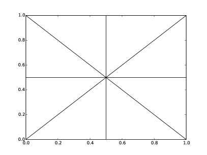
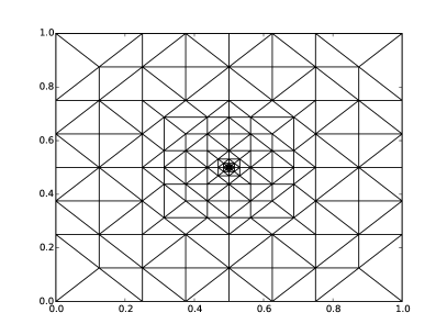
Figure 3: Initial and six times refined meshes in the point load case.

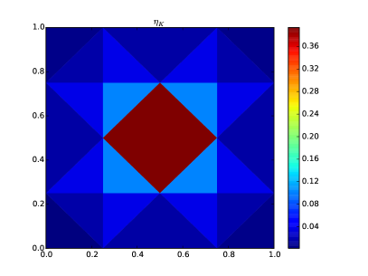
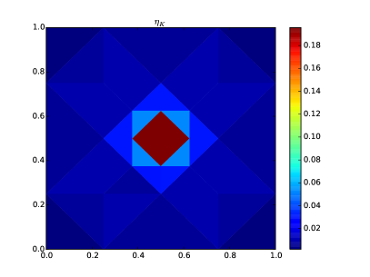
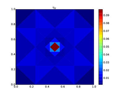
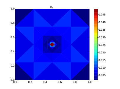
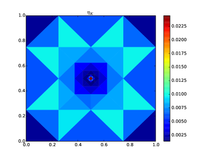
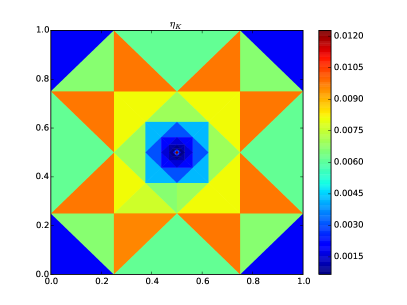
Figure 4: Elementwise error estimators in the point load case.

Figure 5: The results of the point load case.

Figure 6: The efficiency of the estimator in the point load case. The normalization parameter $c$ is chosen as the mean value of the ratio $\eta/{\left|\kern-1.07639pt\left|\kern-1.07639pt\left|u-u_{h}\right|\kern-1.07639pt\right|\kern-1.07639pt\right|}$.

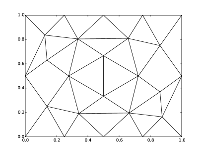
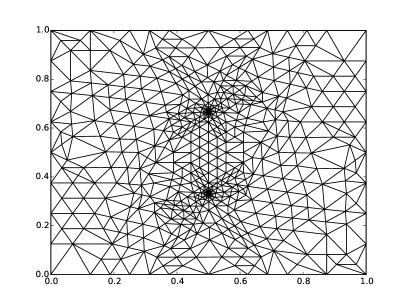
Figure 7: Initial and 6 times refined meshes for the line load case.

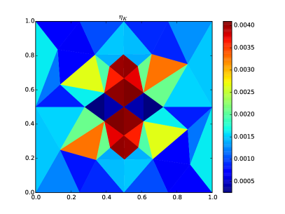
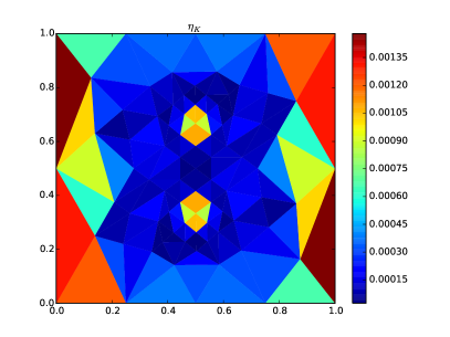
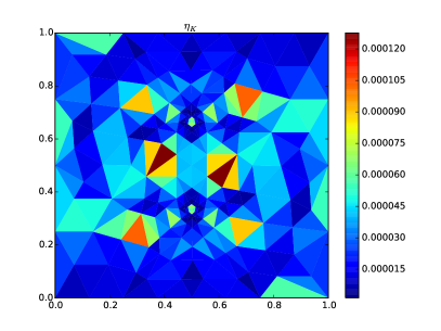
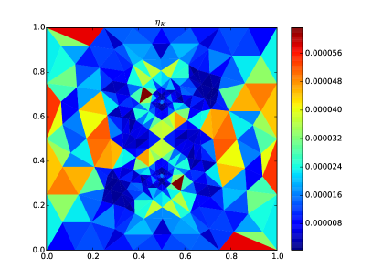
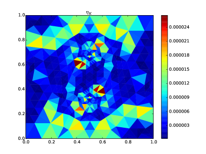
Figure 8: Elementwise error estimators for the line load case.

Figure 9: Results of the line load case.

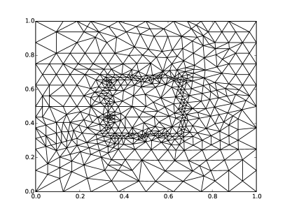
Figure 10: Initial and 8 times refined meshes for the square load case.

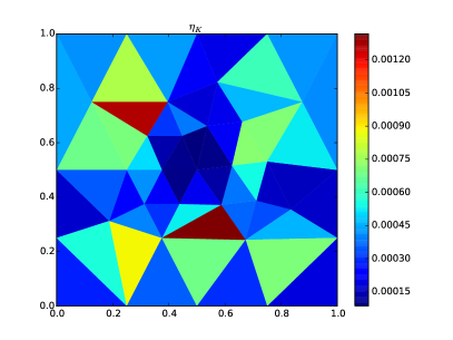
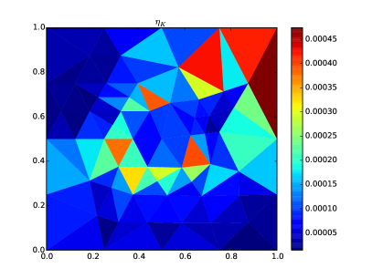
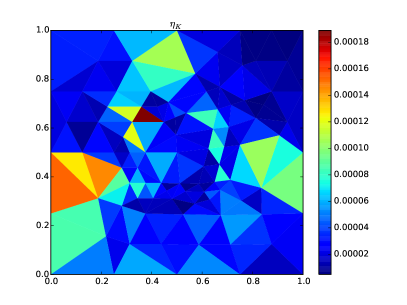
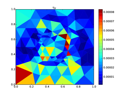
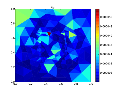
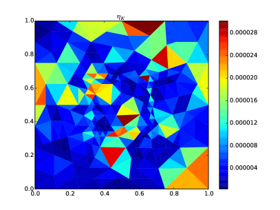
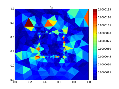
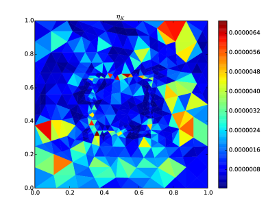
Figure 11: Elementwise error estimators in the square load case.

Figure 12: Results of the square load case.

5.2 L-shaped domain

Next we solve the Kirchhoff plate problem in L-shaped domain with uniform loading $f=1$ and the following three sets of boundary conditions:

1. Simply supported on all boundaries.

2. Clamped on all boundaries.

3. Free on the edges sharing the re-entrant corner and simply supported along the rest of the boundary.

Due to the presence of a re-entrant corner, the solutions belong to $H^{2.33}(\Omega)$, $H^{2.54}(\Omega)$ and $H^{2.64}(\Omega)$ in the cases 1, 2 and 3, respectively(see [23]). As before, we use fifth-order Argyris elements to demonstrate the effectiveness of the adaptive solution strategy. The initial and the final meshes are shown in Fig. 13. The resulting total error estimators and unknown counts are visualized in Fig. 14.

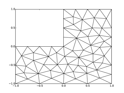
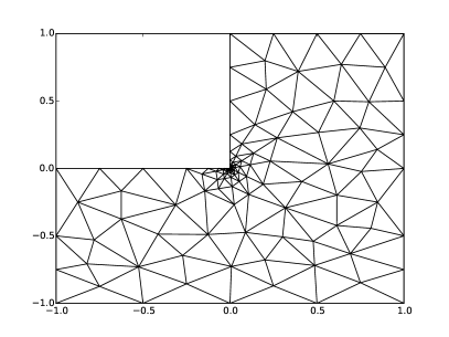
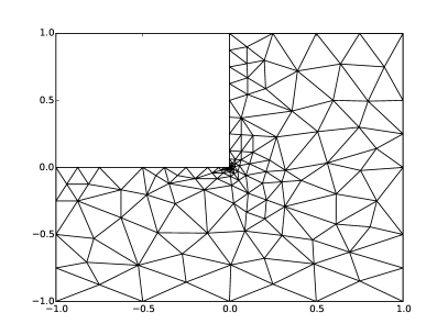
Figure 13: The initial (top right) and the final meshes with different boundary conditions. The boundary conditions at the re-entrant corner are either simply supported (top right), clamped (bottom left) or free (bottom right). Surprisingly enough, the meshes for the simply supported and clamped boundaries end up being exactly the same.

Figure 14: L-shaped domain results. Simply supported (top), clamped (middle) and free (bottom) boundary conditions on the re-entrant corner.

References

• [1] I. Babuška and A. K. Aziz, Survey lectures on the mathematical foundations of the finite element method, Academic Press, New York, 1972, pp. 1–359. With the collaboration of G. Fix and R. B. Kellogg.
• [2] I. Babuška and T. Scapolla, Benchmark computation and performance evaluation for a rhombic plate bending problem, Internat. J. Numer. Methods Engrg., 28 (1989), pp. 155–179, https://doi.org/10.1002/nme.1620280112.
• [3] L. Beirão da Veiga, J. Niiranen, and R. Stenberg, A family of $C^{0}$ finite elements for Kirchhoff plates. I. Error analysis, SIAM J. Numer. Anal., 45 (2007), pp. 2047–2071, https://doi.org/10.1137/06067554X.
• [4] L. Beirão da Veiga, J. Niiranen, and R. Stenberg, A family of $C^{0}$ finite elements for Kirchhoff plates. II. Numerical results, Comput. Methods Appl. Mech. Engrg., 197 (2008), pp. 1850–1864, https://doi.org/10.1016/j.cma.2007.11.015.
• [5] L. Beirão da Veiga, J. Niiranen, and R. Stenberg, A posteriori error analysis for the Morley plate element with general boundary conditions, Internat. J. Numer. Methods Engrg., 83 (2010), pp. 1–26.
• [6] H. Blum and R. Rannacher, On the boundary value problem of the biharmonic operator on domains with angular corners, Math. Methods Appl. Sci., 2 (1980), pp. 556–581, https://doi.org/10.1002/mma.1670020416.
• [7] S. C. Brenner, ${C}^{0}$ Interior penalty methods, in Frontiers in Numerical Analysis–Durham 2010, J. Blowey and M. Jensen, eds., vol. 85 of Lecture Notes in Computational Science and Engineering, Springer-Verlag, 2012, pp. 79–147.
• [8] S. C. Brenner, T. Gudi, and L.-y. Sung, An a posteriori error estimator for a quadratic $C^{0}$-interior penalty method for the biharmonic problem, IMA J. Numer. Anal., 30 (2010), pp. 777–798, https://doi.org/10.1093/imanum/drn057.
• [9] A. Charbonneau, K. Dossou, and R. Pierre, A residual-based a posteriori error estimator for the Ciarlet-Raviart formulation of the first biharmonic problem, Numer. Methods Partial Differential Equations, 13 (1997), pp. 93–111, https://doi.org/10.1002/(SICI)1098-2426(199701)13:1<93::AID-NUM7>3.3.CO;2-G.
• [10] P. G. Ciarlet, The finite element method for elliptic problems, North-Holland Publishing Co., Amsterdam-New York-Oxford, 1978. Studies in Mathematics and its Applications, Vol. 4.
• [11] P. G. Ciarlet and P.-A. Raviart, A mixed finite element method for the biharmonic equation, Math. Res. Center, Univ. of Wisconsin-Madison, Academic Press, New York, 1974, pp. 125–145. Publication No. 33.
• [12] K. Feng and Z.-C. Shi, Mathematical theory of elastic structures, Springer-Verlag, Berlin; Science Press, Beijing, 1996. Translated from the 1981 Chinese original, Revised by the authors.
• [13] B. M. Fraeijs de Veubeke, A course in elasticity, vol. 29 of Applied Mathematical Sciences, Springer-Verlag, New York-Berlin, 1979. Translated from the French by F. A. Ficken.
• [14] E. H. Georgoulis, P. Houston, and J. Virtanen, An a posteriori error indicator for discontinuous Galerkin approximations of fourth-order elliptic problems, IMA Journal of Numerical Analysis, 31 (2011), https://doi.org/10.1093/imanum/drp023.
• [15] V. Girault and L. R. Scott, Hermite interpolation of nonsmooth functions preserving boundary conditions, Math. Comp., 71 (2002), pp. 1043–1074, https://doi.org/10.1090/S0025-5718-02-01446-1.
• [16] W. Gong, G. Wang, and N. Yan, Approximations of elliptic optimal control problems with controls acting on a lower dimensional manifold, SIAM Journal on Control and Optimization, 52 (2014), https://doi.org/10.1137/13091213X.
• [17] T. Gudi, Residual-based a posteriori error estimator for the mixed finite element approximation of the biharmonic equation, Numer. Methods Partial Differential Equations, 27 (2011), pp. 315–328, https://doi.org/10.1002/num.20524.
• [18] T. Gudi and K. Porwal, A $C^{0}$ interior penalty method for a fourth-order variational inequality of the second kind, Numer. Methods Partial Differential Equations, 32 (2016), pp. 36–59, https://doi.org/10.1002/num.21983.
• [19] P. Hansbo and M. G. Larson, A posteriori error estimates for continuous/discontinuous Galerkin approximations of the Kirchhoff-Love plate, Comput. Methods Appl. Mech. Engrg., 200 (2011), pp. 3289–3295, https://doi.org/10.1016/j.cma.2011.07.007.
• [20] J. Hu and Z. Shi, A new a posteriori error estimate for the Morley element, Numer. Math., 112 (2009), pp. 25–40, https://doi.org/10.1007/s00211-008-0205-3.
• [21] X. Huang and J. Huang, A reduced local $C^{0}$ discontinuous Galerkin method for Kirchhoff plates, Numer. Methods Partial Differential Equations, 30 (2014), pp. 1902–1930, https://doi.org/10.1002/num.21883.
• [22] X. Huang and J. Huang, A Superconvergent $C^{0}$ Discontinuous Galerkin Method for Kirchhoff Plates: Error Estimates, Hybridization and Postprocessing, Journal of Scientific Computing, 69 (2016), https://doi.org/10.1007/s10915-016-0232-7.
• [23] H. Melzer and R. Rannacher, Spannungskonzentrationen in Eckpunkten der vertikal belasteten Kirchhoffschen Platte, Bauingenieur, 55 (1980), pp. 181–189.
• [24] J. Nečas and I. Hlaváček, Mathematical theory of elastic and elasto-plastic bodies: an introduction, vol. 3 of Studies in Applied Mechanics, Elsevier Scientific Publishing Co., Amsterdam-New York, 1980.
• [25] J. Shewchuk, Triangle: Engineering a 2D quality mesh generator and Delaunay triangulator, Applied computational geometry towards geometric engineering, (1996), pp. 203–222.
• [26] P. Šolín, Partial differential equations and the finite element method, Pure and Applied Mathematics (New York), Wiley-Interscience [John Wiley & Sons], Hoboken, NJ, 2006.
• [27] S. P. Timoshenko, History of strength of materials. With a brief account of the history of theory of elasticity and theory of structures, McGraw-Hill Book Company, Inc., New York-Toronto-London, 1953.
• [28] S. P. Timoshenko and S. Woinowsky-Krieger, Theory of Plates and Shells., McGraw-Hill Book Company, Inc., New York-Toronto-London, 2 ed., 1959.
• [29] R. Verfürth, A posteriori error estimation techniques for finite element methods, Numerical Mathematics and Scientific Computation, Oxford University Press, Oxford, 2013, https://doi.org/10.1093/acprof:oso/9780199679423.001.0001.
• [30] Y. Xu, J. Huang, and X. Huang, A posteriori error estimates for local $C^{0}$ discontinuous Galerkin methods for Kirchhoff plate bending problems, J. Comput. Math., 32 (2014), pp. 665–686, https://doi.org/10.4208/jcm.1405-m4409.