The optical vs. mid-infrared spectral properties of 82 Type 1 AGNs: coevolution of AGN and starburst

Abstract

We investigated the connection between the mid-infrared (MIR) and optical spectral characteristics in a sample of 82 Type 1 active galactic nuclei (AGNs), observed with Infrared Spectrometer on Spitzer (IRS) and Sloan Digital Sky Survey (SDSS, DR12). We found several interesting correlations between optical and MIR spectral properties: i) as starburst significators in MIR increase, the EWs of optical lines H$\beta$NLR and FeII, increase as well; ii) as MIR spectral index increases, EW([OIII]) decreases, while fractional contribution of AGN (RAGN) is not connected with EW([OIII]); iii) The log([OIII]5007/$\rm H\beta$NLR) ratio is weakly related to the fractional contribution of polycyclic aromatic hydrocarbons (RPAHs). We compare the two different MIR and optical diagnostics for starburst contribution to the overall radiation (RPAH and BPT diagram, respectively). The significant differences between optical and MIR starburst diagnostics were found. The starburst influence to observed correlations between optical and MIR parameters is discussed.

1 Introduction

Understanding the nature of coexistence of active galactic nuclei (AGN) and surrounding starburst (SB) is one of the main problems of galactic evolution. Coexistence of AGNs and SBs is found in various samples such as hyperluminous infrared (IR) galaxies (Ruiz et al., 2013), ultra(luminous) IR galaxies (Kirkpatrick et al., 2015), Seyfert 1 and Seyfert 2 galaxies (Dixon & Joseph, 2011), studied in models (Lipari & Tarlevich, 2006) and often discussed in the frame of AGN spectral properties (Mao et al., 2009; Sani et al., 2010; Popović & Kovačević, 2011; Feltre et al., 2013; Melnick et al., 2015; Ishibashi & Fabian, 2016; Contini, 2016). There are some indications that AGNs may suppress star formation and gas cooling (Croton et al., 2006; Man et al., 2016), and that star formation is higher in AGNs with lower black hole (BH) mass (Sani et al., 2010). Nevertheless, some studies show a correlation between star formation rate and AGN luminosity, at high luminosity AGNs (Lutz et al., 2010; Bonfield et al., 2011).

To find SB contribution to the AGN emission there are several methods in the optical and MIR spectrum. The empirical separation between the low-ionization nuclear emission-line regions (LINERs), HII regions and AGNs at the optical wavelengths is the BPT diagram (Baldwin et al., 1981; Kewley et al., 2001; Kauffmann et al., 2003), usually given as the plot of the flux ratio of forbidden and allowed narrow lines log($\rm[NII]6563/H\alpha NLR$) vs. log($\rm[OIII]5007/H\beta NLR$). The main diagnostic assumption is that HII regions are ionized by young massive stars, while AGNs are ionized by high energetic photons emitted from the accretion disc. In the case that the H$\alpha$ spectral range is not present in the AGN spectra, the R=log([OIII]5007/$\rm H\beta$NLR) ratio may indicate the contribution of SB to the AGN emission, as e.g. Popović & Kovačević (2011) suggested that the dominant SBs have R$<$0.5, while dominant AGNs have R$>$0.5.

Mid-infrared (MIR) based probes for the star formation suffer much less from the extinction than ultraviolet, optical and near-IR observations. The first comparison between Type 1 and Type 2 AGNs at 2-11 $\mu$m range is done by Clavel et al. (2000). The star-forming galaxies are expected to have stronger polycyclic aromatic hydrocarbon (PAH) features (Förster Schreiber et al., 2004; Peeters et al., 2004; Wu et al., 2009). Förster Schreiber et al. (2004) tested the relation between both 5-8.5$\mu$m PAH and 15$\mu$m continuum emission with Lyman continuum and found that MIR dust emission is a good tracer for the star formation rate. Shipley et al. (2016) used the H$\alpha$ emission to calibrate PAH luminosity as a measure of a star formation rate.

Brandl et al. (2006) and Dixon & Joseph (2011) discussed the discrimination of SBs from AGNs using the $\rm F_{15\mu m}/F_{30\mu m}$ continuum flux ratio. SBs have steeper MIR spectrum since AGNs produce a warm dust component in MIR (Dixon & Joseph, 2011). The $\rm F_{15\mu m}/F_{30\mu m}$ ratio measures the strength of the warm dust component in galaxies and therefore reflects SB/AGN contribution. Veilleux et al. (2009) have similar conclusion, that SB galaxies have log($\rm F_{\rm 30\mu m}/F_{\rm 15\mu m}$) of 1.55, while AGNs have log($\rm F_{\rm 30\mu m}/F_{\rm 15\mu m}$) of 0.2. As a consequence, 6.2$\mu$m PAH equivalent widths (EWs) correlate with 20-30$\mu$m spectral index (Deo et al., 2007). A lower 25 to 60 $\mu$m flux ratio in SB galaxies than in Seyfert galaxies is explained by cooler dust temperature in SB galaxies. The higher PAH EWs in SB galaxies than in Seyfert galaxies is due to the PAH destruction from the high energetic radiation from the AGN accretion disc (Wu et al., 2009). Another reason for PAH absence in luminous AGNs is a strong MIR continuum that can wash-out the PAH features, reducing their EWs (Laurent et al., 2000; Alonso-Herrero et al., 2014).

MIR lines that could indicate an AGN presence are [NeV]14.32, [NeV]24.3, [SIV]10.51$\mu$m (Spinoglio & Malkan, 1992; Dixon & Joseph, 2011; Chen & Shan, 2014), [OIV]25.9$\mu$m can originate both from starforming regions or AGNs (Lutz et al., 1998a; Wu et al., 2009), while nearby [FeII]25.99$\mu$m is primarily due star formation (Hartigan et al., 2004; Weedman et al., 2005). [NeII]12.8$\mu$m is strong in SB galaxies, but weak in AGNs (Dixon & Joseph, 2011). Therefore, Genzel et al. (1998); Lutz et al. (1998a); Deo et al. (2007) and Dixon & Joseph (2011) used various methods to distinguish AGNs from SBs: [NeIII]15.6$\mu$m/[NeII]12.8$\mu$m, [NeV]14.3$\mu$m/[NeII]12.8$\mu$m, [NeV]24.3$\mu$m/[NeII]12.8$\mu$m, [OIV]25.9$\mu$m/[NeII]12.8$\mu$m, [OIV]25.9/[SIII]33.48 ratios, as well as a fit to the MIR spectral-slope and strength of the PAH features.

There is a number of correlations between the UV, optical and IR spectral properties that can be caused by physical characteristics of AGNs, but also by contribution of SB to the AGN emission. Some of these correlations can be an indicator of SB and AGN coevolution. Note here shortly the results of Boroson & Green (1992) (BG92 afterwards), who performed principal component analysis (PCA) on various AGN optical, radio and X-ray characteristics. They found a set of correlations between different spectral parameters, projected to eigenvector 1 (EV1). Some of these are anticorrelations EW([OIII]) vs. EW(FeII) and full width at half maximum (FWHM) of $\rm H\beta_{broad}$ vs. EW(FeII) at optical wavelengths. These correlations in AGN spectral properties are very intriguing and their physical background is not understood. Other authors performed PCA in different AGN samples in order to explain these correlations (Grupe, 2004; Mao et al., 2009). Wang et al. (2006) and Popović & Kovačević (2011) suggested that the SB affects EV1, while Feng et al. (2015b) found that PAH characteristics are correlated with EV1. Bian et al. (2016) performed PCA on Spitzer spectra of QSOs and compared these results with the ones from BG92.

Many authors have compared the optical and MIR observations of AGNs (see e.g. Sajina et al., 2008; Sani et al., 2010; Lacy et al., 2013; Vika et al., 2017). O’Dowd et al. (2009) and LaMassa et al. (2012) compared the BPT diagram classification and MIR AGN/SB diagnostics and concluded that the congruence is high. On the other hand, Vika et al. (2017) showed that the optical BPT AGN classification does not always match the one obtained from spectral energy distribution (SED) fitting from UV to far-infrared (FIR) wavelengths. Goulding & Alexander (2009) and Dixon & Joseph (2011) used Spitzer data and found that there may exist AGNs in half of the luminous IR galaxies without any evidence of AGN at near-infrared and optical wavelengths, undetected because of the extinction.

At the MIR wavelength range one can see hot, AGN heated dust component, from the pc-size region surrounding the central BH, that could be the reservoir that feeds the central BH during the accretion phase (Feltre et al., 2013). At the optical observations of Type 1 AGNs, the contributions of accretion disc and broad line region are seen. However, the optical and MIR emission of an AGN should be related, as e.g. if the emission of central continuum source is stronger, one can expect that the inner part of torus is larger (Barvainis et al., 1987). Therefore, the correlations between MIR and optical emission in these objects were expected and found (Shao et al., 2013; Singal et al., 2016).

In this work we use optical (SDSS) and MIR (Spitzer) data to investigate the correlations between optical and MIR emission of Type 1 AGNs, and compare the influence of SB/AGN to the optical and MIR spectra. The paper is organized as follows: in Section 2, we describe our sample of Type 1 AGNs, in Section 3 we explain our data analysis for optical and MIR, in Section 4 we present the results, in Section 5 we discuss our results, and in Section 6 we outline our conclusions.

2 The sample

2.1 The sample of Type 1 AGNs

In this research, we used the sample of Type 1 AGNs, found in the cross-match between optical Sloan Digital Sky Survey (SDSS) spectra and MIR Spitzer Space Telescope spectral data.

The SDSS Data Release 12 (DR12) (Alam et al., 2015) contains all SDSS observations until July 2014. These observations were done with 2.5 m telescope at the Apache Point Observatory with two optical spectrograph (SDSS-I and BOSS). All data from prior data releases are included in DR12 and re-analyzed, so that it contains in total 477,161 QSO and 2,401,952 galactic optical spectra. The SDSS-I spectra covering the wavelength range of 3800 Å to 9200 Å with spectral resolution 1850–2200, while BOSS spectra are observed in the range 3650-10400 Å, with spectral resolution of 1560–2650.

IR data used in this work are reduced and calibrated 5-35 $\mu$m IRS spectra, available in the $\rm 6^{th}$ version of The Cornell Atlas of Spitzer/IRS Sources (CASSIS) database, in low-resolution of $\rm R\sim 60-127$ (Houck et al., 2004; Werner et al., 2004; Lebouteiller et al., 2010, 2011).

To find the sample for this investigation, we used Structural Query Language (SQL) to search for all galaxies and quasars in SDSS DR12 which satisfy following criteria:

1. $S/N>$15 in g–band (4686Å), in order to obtain the spectra of an adequate quality for fitting procedure,

2. $z<0.7$, with $z_{warning}$=0 matching the spectra which cover the optical range near the H$\beta$ line,

3. the objects are classified as ’QSO’ or ’galaxy’ in SDSS spectral classification.

The resulting search contained 135,633 objects. These objects were cross-matched in TOPCAT with the latest (from November 2015) Spitzer catalog – Infrared Database of Extragalactic Observables from Spitzer (IDEOS) of 3361 extragalactic sources (Hernán-Caballero et al., 2016). This cross-match resulted with 585 objects. From that sample we selected Type 1 AGN by visual inspection of the optical spectra, removing all objects which do not have broad emission lines in the $\lambda\lambda$4000-5500 Å range. That resulted with 98 Type 1 AGNs. Additionally, 16 objects were removed from the sample because of high noise and/or poor fitting of IR spectra (see Section 3.2). Finally, the sample contains 82 AGN Type 1, with optical and MIR spectra of satisfactory quality (see Table 1). The angular size distances are given in the column (7), while the projected linear diameters of the IRS and SDSS apertures are given in the columns (8) and (9). The distributions of the SDSS and IRS aperture projections for Type 1 sample are given in the Fig. 1, on the two panels – left. The SDSS aperture size is 3^′′ (Rosario et al., 2013), while we took 4.7^′′ for the IRS aperture (Houck et al., 2004).

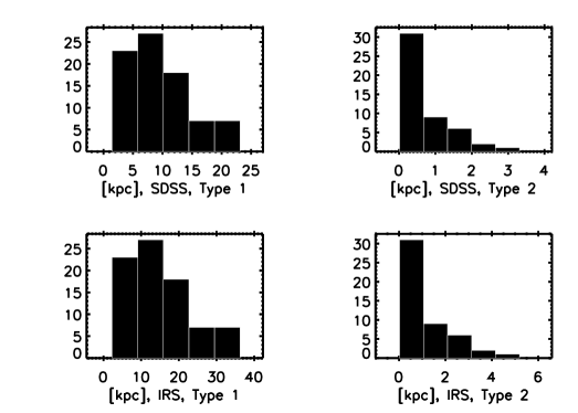
Figure 1: The distributions of the SDSS and IRS aperture projections for the Type 1 AGN sample are given on the left, while the distributions of the SDSS and IRS aperture projections for the Type 2 AGN sample are given on the right.

Table 1: The sample of Type 1 AGNs, observed at the MIR and optical wavelengths. A full version is available at the electronic format.

NED name	RA[∘]	Dec[∘]	SDSS name	plate-MJD-fiber	Z	Distance [Mpc]	SDSSProjA [kpc]	IRSProjA [kpc]
(1)	(2)	(3)	(4)	(5)	(6)	(7)	(8)	(9)
MRK_0042	178.42407	46.21174	J115341.78+461242.25	1446-53080-0129	0.0243	101.0	1.47	2.30
SBS_1301+540	195.99791	53.79165	J130359.48+534729.8	6760-56425-0390	0.0301	124.3	1.81	2.83
MRK_0290	233.96835	57.90264	J153552.40+575409.50	0615-52347-0108	0.0302	124.7	1.81	2.84
UM_614	207.47018	2.07919	J134952.84+020445.10	0530-52026-0165	0.0329	135.4	1.97	3.08
MRK_0836	224.75565	61.23155	J145901.36+611353.59	0611-52055-0437	0.0389	158.9	2.31	3.62

Notes. In the column (1) we give NED name, in the columns (2) and (3) – Right Ascention and the Declination in the arc degrees, in the columns (4) and (5) – SDSS name and plate-MJD-fiber numbers, respectively. In the column (6) is the redshift, column (7) – Angular size distance, calculated using http://www.astro.ucla.edu/Ẽwright/CosmoCalc.html, column (8) – Projected SDSS aperture diameter and column (9) – Projected IRS aperture diameter.

2.2 The sample of Type 2 AGNs from the literature

Because of the difficulties in decomposition of the narrow H$\alpha$, H$\beta$ and [NII] lines in the initial sample of Type 1 AGNs, to check some relations between narrow lines, we also consider a sample of Type 2 AGNs, taken from the literature (more in Section 4.4). The sample is taken from Hernán-Caballero et al. (2015) and García-Bernete et al. (2016), as these authors performed the fitting of CASSIS spectra of $\sim$150 objects – Seyfert 2 galaxies, LINERs and HII regions, using deblendIRS routine (we use the same routine in this work). We took the fitting results that they obtained (spectral index, $\alpha$ and fractional contributions of AGN and PAH in the spectra – RAGN and RPAH, respectively) for all objects for which we found the log([OIII]/H$\beta$) and log([NII]/H$\alpha$) measurements in the other literature. The sample has 49 Type 2 AGNs and the data that we use are given in the Table 2. The angular size distances are given in the column (9), while the projected linear diameters of the IRS and SDSS apertures are given in the columns (10) and (11). The distribution of these aperture projections is given on the Fig. 1, on the two panels – right.

Table 2: The sample of Type 2 AGNs taken from the literature and the data that have been used in this work. A full version is available at the electronic format.

ID	$\alpha$	RPAH	RAGN	log([OIII]/H$\beta$)	log([NII]/H$\alpha$)	Refopt	RefIR	Distance [Mpc]	SDSSProjA [kpc]	IRSProjA [kpc]
(1)	(2)	(3)	(4)	(5)	(6)	(7)	(8)	(9)	(10)	(11)
NGC1052	-2.46	0.053	0.787	0.303	0.079	Ho97	Her15	21.283	0.019	0.029
NGC1275	-2.80	0.0	1.000	1.173	0.134	Ho97	Her15	73.778	1.073	1.681
NGC1386	-2.18	0.130	0.734	1.570	0.200	Kewle01	Her15	12.376	0.180	0.282
NGC1614	-2.54	0.702	0.298	-0.090	-0.220	Kewle01	Her15	66.789	0.971	1.521
NGC1808	-1.66	0.949	0.047	-0.796	-0.268	Gould09	Her15	14.076	0.205	0.321

Notes. In column (1) are object names, in columns (2)-(4) are MIR measurements from the literature, in columns (5)-(6) are optical spectroscopic data from the literature, column (7) – reference for the optical data, column (8) – reference for the MIR data, column (9) – Angular size distance, calculated using http://www.astro.ucla.edu/Ẽwright/CosmoCalc.html, column (10) – Projected SDSS aperture diameter and column (11) – Projected IRS aperture diameter. Feng15b=Feng et al. (2015a), Gar16=García-Bernete et al. (2016), Haas07=Haas et al. (2007), Her15=Hernán-Caballero et al. (2015), Ho97=Ho et al. (1997), Kewle01=Kewley et al. (2001), LaMassa=LaMassa et al. (2011), Gould09=Goulding & Alexander (2009), Shi10=Shields & Filippenko (1990), Veilleux95=Veilleux et al. (1995).

3 Analysis

3.1 AGN optical properties

The SDSS spectra were corrected for the Galactic extinction by using the standard Galactic-type law (Howarth, 1983) for optical-IR range and Galactic extinction coefficients given by Schlegel et al. (1998), available from the NASA/IPAC Infrared Science Archive (IRSA). Afterwards, the spectra were corrected for cosmological redshift and host galaxy contribution (Section 3.1.1), and fitted using model of optical emission in $\lambda\lambda$4000-5500 Å and $\lambda\lambda$6200-6950 Å ranges (Section 3.1.2).

3.1.1 Host galaxy subtraction

To determine the host galaxy contribution in the optical spectra we applied the PCA (Francis et al., 1992; Vanden Berk et al., 2006). PCA is a statistical method which enables a large amount of data to be decomposed and compressed into independent components. In the case of the spectral PCA, these independent components are eigenspectra, whose linear combination can reproduce the observed spectrum. Spectral principal component analysis is commonly used for classification of galaxies and QSOs (Francis et al., 1992; Connolly et al., 1995; Yip et al., 2004a, b, etc.). Yip et al. (2004a) used 170,000 galaxy SDSS spectra to derive the set of the galaxy eigenspectra, while Yip et al. (2004b) used 16,707 QSO SDSS spectra to construct several sets of eigenspectra which describe the QSO sample in different redshift and luminosity bins.

Vanden Berk et al. (2006) introduced the application of this method for spectral decomposition into pure-host and pure-QSO part of an AGN spectrum. This technique assumes that the composite, observed spectrum can be reproduced well by the linear combination of two independent sets of eigenspectra derived from the pure-galaxy and pure-quasar samples. They applied different sets of galaxy and QSO eignespectra derived in Yip et al. (2004a, b), and found that the first few galaxy and quasar eigenspectra can reasonably recover the properties of the sample.

Following the procedure described in Vanden Berk et al. (2006), we used the first 10 QSO eigenspectra derived from high-luminosity (C1), low-redshift range (ZBIN 1), defined by Yip et al. (2004b), and the first 5 galaxy eigenspectra derived in Yip et al. (2004a). The galaxy eigenspectra are downloaded from SDSS Web site, while the QSO eigenspectra are obtained in the private communication (Yip,, 2016).

Figure 2: An example of the spectral PCA decomposition of object SDSS J163631.28$+$420242.5 (0628-52083-0302) on the pure host and the pure QSO part.

Figure 3: An example of the spectral PCA decomposition of object J005812.85+160201.37 (0421-51821-0329) which we fitted only with QSO eigenvectors, without galaxy eigenvectors.

First, we re-bined the observed spectra and 15 eigenspectra to have the same range and wavelength bins. Afterwards, we fitted our spectra with a linear combination of QSO and galaxy eigenspectra. The host part of the spectrum is derived as a linear combination of galaxy, while the AGN part as a linear combination of QSO eigenspectra. We masked all narrow emission lines from the host galaxy part, and subtract only the host galaxy continuum and stellar absorption lines from the observed spectra. Finally, we performed the fitting on that spectra. Our model is described in the Section 3.1.2, while measuring of optical parameters is explained in Section 3.1.3. The example of spectral PCA decomposition is shown in Fig. 2. The host fraction, F_H is measured in the $\lambda\lambda$4160-4210Å range, and presented in Table 3.

In some cases, the fitting results may give a non-physical solutions, such as negative host or AGN part. Vanden Berk et al. (2006) also had non-physical solutions in their Table 2. In our sample we had several objects where fit gives the negative host contribution. In these cases, we assumed that the host part is equal to zero, therefore we excluded galaxy eigenvectors from our fitting and fitted only with the QSO eigenvectors, since we find that these fits are usually good in the part of the spectra we were interested in (see Fig. 3).

3.1.2 Model of the line spectra in the optical range

After the host galaxy contribution is subtracted from the observed spectra, the power-law SED, typical for the quasars, with the broad and narrow emission lines is obtained. The QSO continuum is estimated using the continuum windows given in Kuraszkiewicz et al. (2002). The points of the continuum level are interpolated and the continuum is subtracted (see Kovačević et al., 2010).

The optical emission lines were fitted in two ranges: $\lambda\lambda$4000-5500 Å in order to cover Balmer lines (H$\beta$, H$\gamma$, H$\delta$), optical FeII and [OIII] $\lambda\lambda$4959, 5007Å lines, and $\lambda\lambda$6200-6950 Å, where H$\alpha$ and [NII] $\lambda\lambda$6548, 6583Å lines are present. For fitting the emission lines we used a model of multi-Gaussian functions (Popović et al., 2004), where each Gaussian is assumed to represent an emission from one emission region (see Kovačević et al., 2010; Kovačević-Dojčinović & Popović, 2015, and references therein.)

Figure 4: An example of the fit of spectrum of SDSS J144825.09$+$355946.6 in the $\lambda\lambda$ 4000-5500Å region. A: The observed spectrum (dots) and the best fit (solid line). B: Decomposition of the emission lines. FeII template is denoted with dashed line.

In this model, the number of the free parameters is reduced assuming that lines or line components, which originate from the same emission region, have the same widths and shifts. Therefore, all narrow lines in considered ranges ([OIII] $\lambda\lambda$4959, 5007Å, narrow Balmer lines, [NII] $\lambda\lambda$6548, 6583Å, etc.) have the same parameters of the widths and shifts, since we assumed that they are originating in the Narrow Line Region (NLR). The [OIII] $\lambda\lambda$4959, 5007Å lines are fitted with an additional component which describes the asymmetry in the wings of these lines, while the flux ratio of the $\lambda$4959:$\lambda$5007Å is taken as 1:2.99 (Dimitrijević et al., 2007). The ratio $\approx 3$ is taken for [NII] doublet components.

The Balmer lines are fitted with three components, one narrow – Narrow Line Region (NLR), and two broad – Intermediate and Very Broad Line Region (ILR and VBLR), see Popović et al. (2004); Bon et al. (2006, 2009); Hu et al. (2008). All ILR components of the Balmer lines have the same widths and shifts. The same is for the VBLR components. Numerous optical FeII lines in the $\lambda\lambda$4000-5500Å range are fitted with the FeII template presented in Kovačević et al. (2010) and Shapovalova et al. (2012). In this FeII model, all FeII lines have the same widths and shifts, while relative intensities are calculated within the different FeII line groups, which have the same lower level of the transition (see Kovačević et al., 2010).

The detailed description of this multi-Gaussian model and the fitting procedure is given in Kovačević et al. (2010) and Kovačević-Dojčinović & Popović (2015). The examples of the best fit in the $\lambda\lambda$4000-5500Å and $\lambda\lambda$6200-6950Å ranges are given in Figs. 4 and  5.

Figure 5: An example of the fit of the SDSS J144825.09$+$355946.6 in the $\lambda\lambda$6200-6950Å region. [NII] and [SII] lines are shown with dashed line.

3.1.3 Measuring the optical spectral parameters

After performing the decomposition, we measured different spectral parameters of all considered optical emission lines and their components.

Kinematic parameters, Doppler widths and velocity shifts of emission lines are directly obtained as a product of fitting procedure. Additionally, we measured the FWHM of broad H$\beta$ (ILR+VBLR component), FWHM(H$\beta$). The EWs of emission lines have been measured with respect to pure QSO continuum (after subtraction of the host contribution) below the lines (see Kovačević et al., 2010). The flux of the pure QSO continuum is measured at $\lambda$5100Å, and continuum luminosity is calculated using the formula given in Peebles (1993), with adopted cosmological parameters: $\Omega_{M}$=0.3, $\Omega_{\Lambda}$=0.7 and $\Omega_{k}$=0, and Hubble constant $\rm H_{0}$=70 km s^-1 Mpc^-1. The mass of the black hole ($\rm M_{BH}$) is calculated using the improved formula from Vestergaard & Peterson (2006), for the host light corrected L₅₁₀₀, given in Feng et al. (2014). All measured properties that we used in this work are given in Table 3. The distributions of measured parameters from optical spectra are given in Fig. 6.

Table 3: The optical parameters that we measured for the sample of 82 Type 1 AGNs. A full version of this table is available at the electronic format.

SDSS name	EWH$\beta$N	EWH$\beta$B	EWFeII	[OIII]/H$\beta$	FWHMH$\beta$	L5100	EW[OIII]∗	[NII]/H$\alpha$	$\rm logM_{BH}$	FH
	Å	Å	Å		km s-1	erg s-1	Å		M⊙
(1)	(2)	(3)	(4)	(5)	(6)	(7)	(8)	(9)	(10)	(11)
J115341.78+461242.25	6.677	81.483	191.858	0.447	776.539	42.538	27.877	-0.284	5.78	0.27
J130359.48+534729.8	5.319	82.889	0.0	1.093	4819.368	42.669	105.285	-0.737	7.44	0.42
J153552.40+575409.50	3.610	76.735	0.0	1.192	4258.708	43.449	86.939	-0.581	7.72	0.14
J134952.84+020445.10	7.327	57.233	87.446	1.276	1659.097	42.957	227.384	-0.333	6.65	0.25
J145901.36+611353.59	6.045	144.537	115.841	0.737	6636.606	42.491	33.989	-0.004	7.62	0.65

Notes. (1) SDSS name, (2) EW(H$\beta$NLR), (3) EW(H$\beta$Broad)=EW(H$\beta$ILR)+EW(H$\beta$VBLR), (4) EW(FeII), (5) log([OIII]5007/H$\beta$NLR), (6) FWHM(H$\beta$), (7) log(L5100)=log of luminosity of AGN at $\lambda$=5100Å, multiplied with 5100, (8) EW[OIII]^∗ is EW for both components of doublet ([OIII] $\lambda$4959Å + [OIII] $\lambda$5007Å), (9) log([NII]6583/H$\alpha$NLR), (10) log of black hole mass, log($\rm M_{BH}$), (11) Host fraction in the $\lambda\lambda$4160-4210Å range, obtained in the decomposition.

3.2 MIR properties of the AGNs

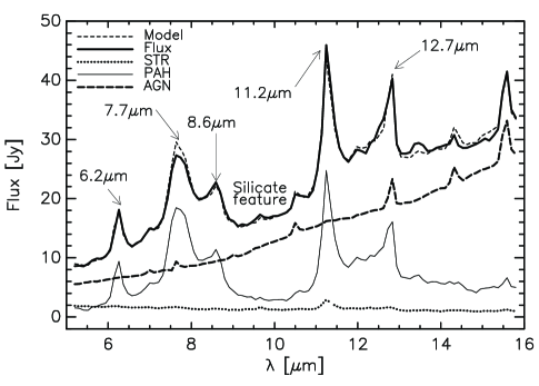
Figure 8: An example of fitting of the IRS spectrum of MRK0662, using deblendIRS software. The spectra is decomposed to the AGN, PAH and stellar component (STR). The PAH and silicate features are marked on the graph.

To study the AGN MIR properties of the sample, we need to disentangle the AGN emission from interstellar PAH, and stellar (STR) components, using some of the existing tools for spectral decomposition of IRS data. We used deblendIRS routine, written in IDL (Hernán-Caballero et al., 2015). Having a collection of real spectral templates, this software chooses the best linear combination of one stellar template, one PAH template, and one AGN template, to model an IRS spectra, only in the spectral range 5.3–15.8$\mu$m. An example of fitting of an IRS spectrum is present on the Fig. 8. For the stellar templates, the routine uses 19 local elliptical and S0 galaxies, the 56 PAH templates are IRS spectra of normal starfoming and SB galaxies at z$\leq$ 0.14, while the AGN templates are 181 IRS spectra of sources classified in the optical as quasars, Seyfert galaxies, LINERs, blazars, optically obscured AGNs and radio galaxies.

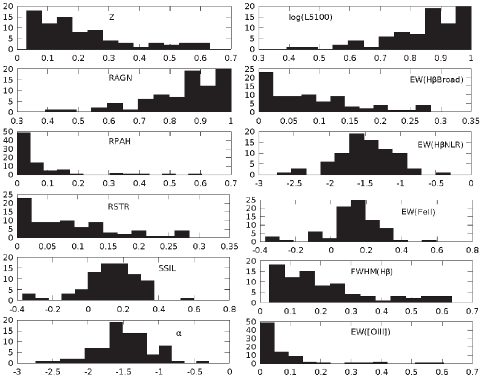
Figure 6: Distribution of redshifts and main obtained parameters from fitting MIR (left) and optical (right) spectra (see the text).

The main fitting results are fractional contributions of AGN, PAH and stellar components to the integrated 5–15$\mu$m luminosity, named RAGN, RPAH and RSTR, respectively (RAGN+RPAH+RSTR=1), spectral index of the AGN component (assuming a power law continuum $f_{\nu}\propto\nu^{\alpha}$, between 8.1 and 12.5$\mu$m), $\alpha$ and the silicate strength of the best fitting AGN template, $\rm S_{SIL}$ (see Hernán-Caballero et al., 2015). They define $\rm S_{SIL}$ as a ln(F($\lambda_{p}$)/F_C($\lambda_{p}$)), where F($\lambda_{p}$) and F_C($\lambda_{p}$) are the flux densities of the spectrum and the underlying continuum, at the wavelength of the peak of the silicate feature. Other results of the fit are flux densities of AGN, PAH and STR components (spectra), names of the used spectral galactic templates, $\chi^{2}$, the coefficient of variation of the rms error ($\rm CV_{RMSE}$), monochromatic luminosities of the source and fractional contribution to the restframe of the AGN component, at 6 and 12$\mu$m. The resulting parameters that we use in this work are given in Table 4, while the distributions of the main parameters is given on the Fig. 6. In these histograms one can see that the AGN contribution is very dominant in the sample, comparing to PAH and stellar emission. Silicate feature is usually in the emission (positive $\rm S_{SIL}$).

From the fitting results we chose 82 successful fits, based on low reduced $\chi^{2}$, $\rm CV_{RMSE}$ (should be $<$0.1; Hernán-Caballero et al., 2015), and the visual inspection. The 16 sources were rejected due to poor fitting, from which 6 are extended sources. All these 82 objects are point sources except one, 0615-52345-0041.

Independently of deblendIRS code, we calculated EWs of PAH features at 7.7 and 11.2 $\mu$m (given in Table 4), using STARLINK software (DIPSO; Howarth & Murray, 1987) on redshift corrected IRS spectra.

Table 4: The MIR parameters that we calculated and measured for the sample of 82 Type 1 AGNs. A full version of this table is available at the electronic format.

NED Name	RAGN	RPAH	$\rm S_{SIL}$	$\alpha$	L6	L12	EW7.7	EW11.2	R30/15	$\rm\chi^{2}_{RED}$	$\rm CV_{RMSE}$
					1042erg s-1	1042erg s-1	$\mu$m	$\mu$m
(1)	(2)	(3)	(4)	(5)	(6)	(7)	(8)	(9)	(10)	(11)	(12)
MRK_0042	0.61	0.303	0.1	-1.443	6.42	7.34	0.690	0.370	0.30	0.53	0.03
SBS_1301+540	0.71	0.024	0.269	-1.447	8.99	7.44	$<$0.01	0.018	0.97	0.16	0.03
MRK_0290	0.89	0.005	0.061	-1.858	3.34	4.24	0.028	0.015	0.73	1.17	0.03
UM_614	0.92	0.023	0.17	-1.656	1.74	2.15	0.007	$<$0.01	0.89	0.73	0.06
MRK_0836	0.62	0.125	0.304	-1.633	6.03	5.90	0.071	0.137	0.43	0.21	0.05

Notes. (1) NED name, (2) and (3) – fractional contributions of the AGN and PAH components to the MIR luminosity, respectively (RAGN+RPAH+RSTR=1), (4) $\rm S_{SIL}$ – strength of a silicate feature, (5) spectral index, (6) and (7) monochromatic luminosities of the source at 6 and 12 $\mu$m, (8) and (9) EWs of the PAH features at 7.7 and 11.2$\mu$m, (10) Ratio of fluxes at 30 and 15$\mu$m, (11) reduced $\rm\chi^{2}$ and (12) $\rm CV_{RMSE}$.

3.3 Broad-line Balmer decrement and nuclear extinction

As can be seen on Figs. 4 and 5, we decompose the H$\alpha$ and H$\beta$ into three components: NLR, ILR and VBLR. The narrow-line Balmer decrement, H$\alpha$ⁿ/H$\beta$ⁿ, is calculated as a flux ratio of H$\alpha$NLR and H$\beta$NLR, while the broad-line Balmer decrement is found as H$\alpha$^b/H$\beta$^b, where H$\alpha$^b and H$\beta$^b are sums of the ILR and VBLR flux components. These fluxes and ratios are given in the Table 5.

The broad-line Balmer decrement is often used for the estimation of the dust extinction in the BLR (Dong et al., 2008; Zhang et al., 2008; Gaskell, 2017). The distribution of broad-line Balmer decrement is given in the histogram on the Fig. 7. They are typically lower than the ones for the submm galaxies from Takata et al. (2006) that have values from 5-20. Obtained H$\alpha$^b/H$\beta$^b ratios are comparable to the values from the large sample of Seyfert 1 galaxies from Dong et al. (2008), that are well described with a log-Gaussian, with a peak at 3.05. The median value of our decrements is 3.76. However, we should note that the other effects can affect the H$\alpha$^b/H$\beta$^b ratio, such as photoionization, recombination, collisions, self-absorption, dust obscuration, etc. (Popović, 2003; Ilić et al, 2012).

If we use the equation (5) from Zhang et al. (2008), we could estimate the minimum color excess, E(B-V), from the sample to be -0.263. For that value of E(B-V), one can use the reddening curve from Calzetti et al. (2000) to calculate the extinction, A_λ at any specific wavelength.

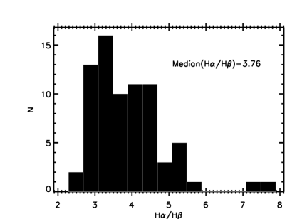
Figure 7: The distribution of broad-line Balmer decrements, H$\alpha$^b/H$\beta$^b, from the Type 1 sample.

Table 5: Flux measurements of the hydrogen recombination lines and obtained Balmer decrements for the Type 1 sample.

Plate-MJD-Fiber	H$\alpha$NLR	H$\beta$NLR	H$\alpha$Broad	H$\beta$Broad	H$\alpha$b/H$\beta$b	H$\alpha$n/H$\beta$n
	10-17erg s-1cm-2	10-17erg s-1cm-2	10-17erg s-1cm-2	10-17erg s-1cm-2
(1)	(2)	(3)	(4)	(5)	(6)	(7)
0276-51909-0251	1.39E+03	3.08E+02	34098.93	1.09E+04	3.13	4.52
0339-51692-0042	7.51E+02	1.16E+02	7841.89	2.26E+03	3.47	6.49
0340-51990-0485	2.86E+02	1.26E+02	19216.24	6.71E+03	2.86	2.27
0355-51788-0408	2.78E+02	5.76E+01	5118.76	1.48E+03	3.46	4.83
0386-51788-0086	9.49E+02	1.86E+02	43266.6	8.57E+03	5.04	5.10

Notes. (1) SDSS Plate-MJD-Fiber, (2) H$\alpha$NLR flux, (3) H$\beta$NLR flux, (4) H$\alpha$Broad flux, (5) H$\beta$Broad flux, (6) H$\alpha$^b/H$\beta$^b – the Balmer decrement of the broad lines, and (7) H$\alpha$ⁿ/H$\beta$ⁿ – the Balmer decrement of the narrow lines.

4 Results

We found that in the Type 1 AGN sample there is relatively small contribution of PAH, of RPAH$<$20%, for the majority of objects (see histogram in Fig. 6).

On the histogram on the Fig. 6, in Type 1 AGN sample we see more silicate emission ($\rm S_{SIL}>$0), than absorption ($\rm S_{SIL}<$0), as mentioned in Weedman et al. (2012) and Stalevski et al. (2011). Hao et al. (2007) suggested that the QSOs are characterized by silicate emission, while Sy1s have equally distributed emission or weak absorption. That is in the agreement with our findings. The silicate feature in the absorption means there is a cooler dust between the observer and the hotter dust responsible for the MIR continuum.

We created a linear correlation matrix for all MIR and optical parameters together. Pearson correlation coefficients and the P-values are given in the Table 6, higher and lower, respectively. Significant correlations are marked with stars.

Table 6: The correlation matrix for the optical and MIR parameters. The higher values are the correlation coefficients, while the lower values are the the P values. The correlations with P$<$0.05 are marked with *. (2) EW(H$\beta$NLR), (3) EW(FeII), (4) log([OIII]5007/H$\beta$NLR), (5) FWHM(H$\beta$), (6) log of luminosity of AGN at $\lambda$=5100Å, multiplied with 5100, (7) EW([OIII]) for both [OIII] components, (8) and (9) RAGN and RPAH – fractional contributions of the AGN and PAH components to the MIR luminosity, respectively, (10) $\rm S_{SIL}$, (11) spectral index, (12) Monochromatic luminosity of the source at 12 $\mu$m, (13) EW of the PAH feature at 7.7$\mu$m, (14) log of black hole mass, (15) Ratio of fluxes at 30 and 15$\mu$m, and (16) EW(H$\beta$Broad).

	EW(H$\beta$NLR)	EW(FeII)	log([OIII]/H$\beta$)	FWHM(H$\beta$)	log(L5100)	EW([OIII])	RAGN	RPAH	$\rm S_{SIL}$	$\alpha$	L12	EW(PAH7.7)	$\rm M_{BH}$	$\rm R_{30/15}$	EW(H$\beta$Broad)
(1)	(2)	(3)	(4)	(5)	(6)	(7)	(8)	(9)	(10)	(11)	(12)	(13)	(14)	(15)	(16)
EW(H$\beta$NLR)	1	0.233*	-0.534*	-0.322*	-0.447*	0.317*	-0.340*	0.385*	0.004	-0.181	-0.311*	0.390*	-0.526*	-0.096	-0.020
EW(H$\beta$NLR)	–	0.035	2.90E-7	0.003	2.49E-5	0.004	0.002	3.51E-4	0.971	0.104	0.004	0.002	3.96E-7	0.490	0.857
EW(FeII)	0.233*	1	-0.479*	-0.324*	-0.185	-0.336*	-0.206	0.315*	-0.156	0.119	-0.008	0.379*	-0.349*	-0.255	0.282*
EW(FeII)	0.035	–	6.10E-6	0.003	0.097	0.002	0.063	0.004	0.160	0.285	0.945	0.003	0.001	0.062	0.010
log([OIII]/H$\beta$)	-0.534*	-0.479*	1	0.300*	0.040	0.443*	0.293*	-0.262*	-0.203	-0.316*	0.104	-0.265*	0.242*	-0.138	0.009
log([OIII]/H$\beta$)	2.90E-7	6.10E-6	–	0.006	0.722	3.41E-5	0.008	0.018	0.069	0.004	0.356	0.039	0.029	0.322	0.937
FWHM(H$\beta$)	-0.322*	-0.324*	0.300*	1	0.153	-0.048	0.094	-0.139	0.147	-0.029	0.161	0.009	0.711*	0.071	0.164
FWHM(H$\beta$)	0.003	0.003	0.006	–	0.169	0.665	0.400	0.213	0.187	0.793	0.149	0.947	7.35E-14	0.609	0.140
log(L5100)	-0.447*	-0.185	0.040	0.153	1	-0.265*	0.549*	-0.540*	0.211	0.310*	0.663*	-0.449*	0.787*	0.374*	-0.080
log(L5100)	2.49E-5	0.097	0.722	0.170	–	0.016	9.08E-8	1.66E-7	0.057	0.004	1.16E-11	2.80E-4	0	0.005	0.473
EW([OIII])	0.317*	-0.336*	0.443*	-0.048	-0.265*	1	0.082	-0.029	-0.207	-0.368*	-0.177	-0.002	-0.182	-0.096	-0.037
EW([OIII])	0.004	0.002	3.41E-5	0.665	0.016	–	0.464	0.797	0.062	6.61E-4	0.112	0.985	0.101	0.489	0.741
RAGN	-0.340*	-0.206	0.293*	0.094	0.549*	0.082	1	-0.823*	0.097	0.293*	0.416*	-0.688*	0.436*	0.292*	-0.161
RAGN	0.002	0.063	0.008	0.400	9.08E-8	0.464	–	0	0.385	0.007	1.03E-4	8.70E-10	4.18E-5	0.032	0.148
RPAH	0.385*	0.315*	-0.262*	-0.139	-0.540*	-0.029	-0.823*	1	-0.180	-0.304*	-0.270*	0.866*	-0.458*	-0.521*	0.013
RPAH	3.51E-4	0.004	0.018	0.213	1.66E-7	0.797	0	–	0.105	0.005	0.014	0	1.52E-5	5.37E-5	0.906
$\rm S_{SIL}$	0.004	-0.156	-0.203	0.147	0.211	-0.207	0.097	-0.180	1	0.228*	0.061	-0.393*	0.201	0.291*	8.15E-4
$\rm S_{SIL}$	0.971	0.160	0.069	0.187	0.057	0.062	0.385	0.105	–	0.039	0.586	0.002	0.070	0.033	0.994
$\alpha$	-0.181	0.119	-0.316*	-0.029	0.310*	-0.368*	0.293*	-0.304*	0.228*	1	0.191	-0.329*	0.200	0.462*	0.010
$\alpha$	0.104	0.285	0.004	0.793	0.004	6.61E-4	0.007	0.005	0.039	–	0.086	0.009	0.072	4.35E-4	0.926
L12	-0.311*	-0.008	0.104	0.161	0.663*	-0.177	0.416*	-0.270*	0.061	0.191	1	-0.162	0.536*	0.024	-0.122
L12	0.004	0.945	0.356	0.149	1.16E-11	0.112	1.03E-4	0.014	0.586	0.086	–	0.213	2.11E-7	0.864	0.274
EW(PAH7.7)	0.390*	0.379*	-0.265*	0.009	-0.449*	-0.002	-0.688*	0.866*	-0.393*	-0.329*	-0.162	1	-0.300*	-0.408*	0.115
EW(PAH7.7)	0.002	0.003	0.039	0.947	2.80E-4	0.985	8.70E-10	0	0.002	0.009	0.213	–	0.019	0.006	0.378
$\rm M_{BH}$	-0.526*	-0.349*	0.242*	0.711*	0.787*	-0.182	0.436*	-0.458*	0.201	0.200	0.536*	-0.300*	1	0.324*	0.065
$\rm M_{BH}$	3.96E-7	0.001	0.029	7.35E-14	0	0.101	4.18E-5	1.52E-5	0.070	0.072	2.11E-7	0.019	–	0.017	0.559
R30/15	-0.096	-0.255	-0.138	0.071	0.374*	-0.096	0.292*	-0.521*	0.291*	0.462*	0.024	-0.408*	0.324*	1	0.149
R30/15	0.490	0.062	0.322	0.609	0.005	0.489	0.032	5.37E-5	0.033	4.35E-4	0.864	0.006	0.017	–	0.283
EW(H$\beta$Broad)	-0.020	0.282*	0.009	0.164	-0.080	-0.037	-0.161	0.013	8.15E-4	0.010	-0.122	0.115	0.065	0.149	1
EW(H$\beta$Broad)	0.857	0.010	0.937	0.140	0.473	0.741	0.148	0.906	0.994	0.926	0.274	0.378	0.559	0.283	–

4.1 Expected and confirmed relations

One of the most expected results is the correlation between the AGN continuum luminosity (L5100) at optical wavelengths and total luminosities at 6 and 12$\mu$m, with $\rho$=0.67 and 0.66, while P$<$0.00001 (Fig. 9). Also, there is the dependence of RAGN and RPAH with L5100, $\rho$=0.55 and -0.54, respectively, with P$<$0.00001, which is shown in numerous works (e.g. Vika et al., 2017).

Another expected relation that we found is that RAGN and RPAH are in trend with redshift; Pearson’ coefficients are $\rho$=0.31; P=0.0038 and $\rho$=-0.24; P=0.03, respectively. Finally, RAGN and RPAH are in trend with the luminosities at 6$\mu$m ($\rho$=0.39, P=0.0003 and $\rho$=-0.27; P=0.014) and at 12$\mu$m ($\rho$=0.41; P=0.0001 and $\rho$=-0.27; P=0.014).

$\rm S_{SIL}$ is only weakly correlated with $\alpha$, with $\rho$=0.228, P=0.039, and that is already shown in the literature (Hernán-Caballero et al., 2015; Hao et al., 2007).

Among known anticorrelations that we expected to obtain is between RPAH and black hole mass, $\rm M_{BH}$ (for example Sani et al., 2010), see Fig. 10. Here we obtained a slight trend with Pearson’ coefficient $\rho$=-0.44, with P=0.00004; PAH may be more dominant in AGNs with lower M_BH.

We obtained expected correlations between EW([OIII]) and EW(FeII) ($\rho$=-0.34; P=0.002), as well as between EW(FeII) and FWHM(H$\beta$) ($\rho$=-0.32; P=0.003, see Fig. 11), which are a part of the EV1 from BG92.

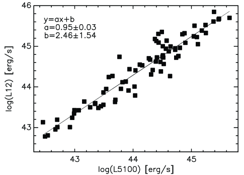
Figure 9: The correlation between the AGN continuum luminosity (L5100) at the optical wavelengths and monochromatic luminosity of the source at 12$\mu$m. The Pearson’ correlation coefficient is $\rho$=0.66; with P$<$ 0.00001. The linear relation between these quantities is given as a solid line and the coefficients $a$ and $b$ are given on the plot.

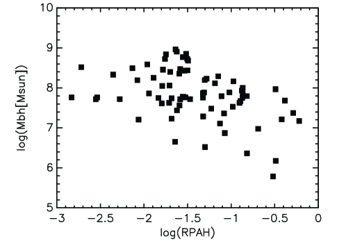
Figure 10: A trend between RPAH and the black hole mass, $\rm M_{BH}$. The Pearson’ correlation coefficient is $\rho$=-0.44; with P=0.00004.

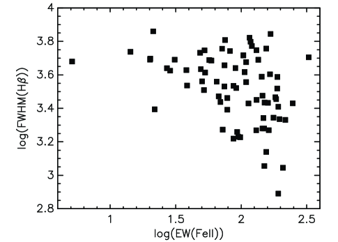
Figure 11: The correlation between EW(FeII) and FWHM(H$\beta$); $\rho$=-0.32; P=0.003; a part of the EV1 from BG92.

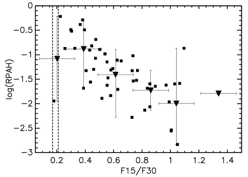
Figure 12: Fractional contribution of PAH component in MIR luminosity, $\rm RPAH$, compared with ratio of fluxes at 15 and 30 $\mu$m, $\rm R_{15/30}$. Vertical dashed lines mark the transition region between AGN and SB, according to Brandl et al. (2006). The Pearson’ correlation coefficient is $\rho$=-0.52; with P= 0.00005. The triangles mark the data in the bins whose widths on the x-axis are 0.25.

4.2 Starbursts at MIR wavelengths

At MIR wavelengths, we may estimate the SB contribution to the total radiation based on the RPAH result. Here, we additionally, compare the RPAH with other two usual methods by which SB is estimated. The first is the ratio of the fluxes at 15 and 30 $\mu$m, the most accurate method, as suggested by Brandl et al. (2006), see Fig. 12. There is a significant correlation between RPAH and this ratio. On this plot, x-axis is divided to the bins of the width 0.25 and binned data are shown with the triangles.

The second criterion is the the strength of some PAH feature; here we present the EWs of the 7.7 and 11.2$\mu$m PAH features, on Fig. 13. There is a significant dependence between EWs and RPAH. As suggested by Lutz et al. (1998a), the objects with EW7.7 $\mu$m $>$1 are SB dominated, while the rest are AGN dominated. On this plot, EW7.7 $\mu$m $>$1 is present only for two objects. Interestingly, only these two objects have RPAH $>$ 50%.

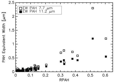
Figure 13: EWs of 7.7 and 11.2$\mu$m PAH features, compared with the fractional contribution of PAH component, RPAH. Pearson’ correlation coefficients are $\rho$=0.87; with P$<$0.0001, and $\rho$=0.89; with P$<$0.0001, for PAHs at 7.7 and 11.2 $\mu$m, respectively.

4.3 Comparison of the optical and MIR parameters

In the correlation matrix (Table 6) there are several trends between the optical and MIR parameters. As SB significators in the MIR (RPAH, EWPAH7.7, EWPAH11.2) increase, EWs of the optical lines FeII and H$\beta$NLR increase, as well. On the other hand, as the MIR spectral index, $\alpha$ increases, a well known AGN indicator, EW([OIII]) decreases ($\rho$=-0.37, P=6.6E^-4), while the EW([OIII]) is not related to the AGN or PAH fraction.

We do not notice any trend of PAH EW or RPAH with the FWHM(H$\beta$) line, as suggested by Sani et al. (2010), who found that narrower broad H$\beta$ lines have a stronger PAH emission in the Type 1 AGNs. However, our later analysis (Section 4.5, 5.3), will show that there is a connection between RPAH and FWHM(H$\beta$).

Considering this comparison it should be emphasized that the BPT and MIR SB/AGN diagnostics do not necessarily trace the contribution of an AGN to the total power of the galaxy. Therefore, there may exist some other effects which can affect one or both diagnostics.

4.4 Comparison between starburst fraction at optical (BPT diagram) and at MIR wavelengths (RPAH)

Traditionally, BPT diagram have been used for optical diagnostics between AGN, composites and SB (Baldwin et al., 1981; Kewley et al., 2001). In Fig. 14 we show the BPT diagram of the Type 1 data sub-sample of 69 objects with available range of 6200-6550Å which covers H$\alpha$ and [NII] lines. To find the real ratio between the AGN and PAH contribution in the MIR spectra and present it on BPT diagram, we excluded stellar contribution, by using the formula RPAH=RPAH/(RPAH+RAGN) from now on. On the diagram, the RPAH is quantified by the three different symbol sizes. Clearly, there are a couple of objects with a low RPAH, that lie below the solid separation curve from Kewley et al. (2001); they should be above that curve, by the optical diagnostics. Similarly, a few SB dominated objects, according to the MIR fitting, lie on the AGN part of BPT diagram. These results suggest that there might be a significant difference between optical and MIR SB quantification.

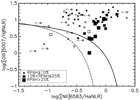
Figure 14: BPT diagram for Type 1 AGN sample where RPAH contribution is illustrated with the symbol size (see the legend). We show only the objects where both narrow H${\alpha}$ and [NII] lines are not zero. Full squares represent the objects where narrow lines H$\alpha$ and [NII] are well detected. Empty squares mark objects where [NII] doublet can not be well resolved within broad H$\alpha$ line, therefore these fits are less confident (see the Appendix A). The arrows mark upper limits of log([NII]6583/H$\alpha$NLR). The dashed line is the separation curve from Kauffmann et al. (2003), while the solid line is the separation curve from Kewley et al. (2001).

To confirm these doubts, taking into account that it is complicated to decompose the narrow lines in the Type 1 AGNs (see the Appendix A and Popović & Kovačević, 2011), we chose a sample of Type 2 AGNs (see Table 2 and Section 2.2). We made another BPT diagram, composed from the various LINER, HII regions and Seyfert 2 galaxies, from the samples of Hernán-Caballero et al. (2015) and García-Bernete et al. (2016). That BPT diagram is shown in the Fig. 15. Again, the symbol size represents RPAH value. Similarly as above, we notice that often these optical and MIR results give different information about SB and AGN ratio.

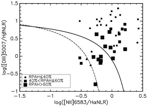
Figure 15: BPT diagram for Type 2 AGN sample where RPAH contribution is illustrated with the symbol size (see the legend). The data are taken from the literature (Table 2). The separation curves are the same as in Fig. 14.

Popović & Kovačević (2011) suggested that one axis of the BPT diagram, the ratio R=log(${\rm[OIII]5007/H\beta}$NLR), may be the significant indicator of the SB activity, where the objects with R$<$0.5 are SB dominated and the rest are AGN dominated. Furthermore, these authors showed that these two groups (R$<$0.5 and R$>$0.5) belong to the different populations of objects, since they show certain different optical characteristics, and that is the essence of the BPT diagram. Therefore, we compare the RPAH (from MIR data) and this ratio $\rm R$, on the Fig. 16 for both Type 1 and Type 2 samples. Here we found quite weak trend of $\rho$=-0.26 and P=0.018 for Type 1 and stronger $\rho$=-0.6 and P=4.77$\times$ 10^-6 correlation for the Type 2 sample. This graph shows that the objects with R$<$0.5 are not always SB dominated (based to MIR data), hence there may be some other reason why they are different at optical wavelengths, or the origin of the optical and MIR radiation may be different. It can be seen in Fig. 16 that, in general, the ratio log(${\rm[OIII]5007/H\beta}$NLR) is decreasing as RPAH is increasing.

One should be aware that this comparison between MIR and optical diagnostics is limited by the factors such as the used data, radiation mechanisms, observed wavelength ranges and power distribution, and therefore these conclusions should not be taken literally.

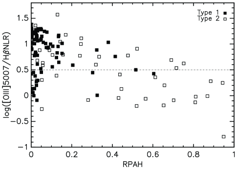
Figure 16: Comparison between RPAH (PAH fraction from MIR data) with log(${\rm[OIII]5007/H\beta}$NLR) (from optical data), for the sample of Type 1 AGNs (Pearson’ correlation coefficient is $\rho$=-0.26; P=0.018) – full squares, and for the sample of Type 2 AGNs ($\rho$=-0.60; P=4.77$\times$ 10^-6) – open squares.

4.5 Principal Component analysis of the spectral parameters

The dependence between all calculated optical and MIR parameters is complex and therefore we used the PC analysis to understand the most important connections. Having our correlation matrix (Table 6), we chose several parameters which should contain a potentially unique information. The optical parameters are: EW([OIII]), EW(FeII), EW(H$\beta$NLR), EW($\rm H\beta_{broad}$) (ILR+VBLR), log([OIII]/H$\beta$NLR), FWHM(H$\beta$) and log($\rm L5100$), which are chosen to be compared with correlations found in the EV1 of BG92. The MIR parameters taken for analysis are: RPAH, $\alpha$ and $\rm S_{SIL}$ (since it is a possible indicator of the AGN geometry or inclination).

The aim of this analysis is:

1. to check possible connections between BG92 EV1 correlations (between EW(FeII) vs. EW([OIII]) and EW(FeII) vs. FWHM(H$\beta$)) and some MIR spectral properties, which could give us some insight in physical cause of these correlations.

2. to compare the RPAH with log([OIII]5007/$\rm H\beta$NLR), in order to clarify the previous results (see Section 4.4) about their inconsistency.

Table 7: PCA of the optical and MIR properties in sample of 82 AGN Type 1.

	Comp.1	Comp.2	Comp.3	Comp.4
Standard deviation	1.617	1.480	1.128	1.037
Proportion of Variance	0.262	0.219	0.127	0.107
Cumulative Proportion	0.262	0.481	0.608	0.715
RPAH	0.447	-0.095	-0.160	-0.109
$\alpha$	-0.140	0.479	0.101	0.087
$\rm S_{SIL}$	-0.149	0.274	0.262	-0.677
EW([OIII])	0.041	-0.530	0.228	-0.079
EW(FeII)	0.370	0.314	-0.348	0.231
EW(H$\beta$NLR)	0.472	-0.052	0.321	-0.304
EW($\rm H\beta_{broad}$)	0.057	0.059	-0.671	-0.280
log([OIII]/H$\beta$NLR)	-0.349	-0.466	-0.192	0.149
FWHM(H$\beta$)	-0.315	-0.092	-0.346	-0.494
log(L5100)	-0.415	0.274	0.108	0.160

For the PCA we used the task princomp with the option cor=true, in R. The results of the PCA are shown in the Table 7. The first four components together account for 71% of the variance. The first two components are the most important underlying parameters that govern the observed properties of the AGN sample. Both, the first and the second eigenvector account for $\approx 20\%$ variance, while each of the next two eigenvectors account for $\approx 10\%$ variance.

The PCA indicates that the first principal component is dominated by RPAH and EW(H$\beta$NLR). While RPAH, EW(H$\beta$NLR) and EW(FeII) have positive projections on the first eigenvector, log([OIII]/H$\beta$NLR), FWHM(H$\beta$) and log$\rm(L5100)$ have negative projections. Therefore, this eigenvector indicates that as the SB contribution, measured in IR, is stronger, EW(H$\beta$NLR), EW(FeII) increase, but the optical luminosity, FWHM(H$\beta$) and log([OIII]/H$\beta$NLR) ratio decrease. It seems that the strongest indicator of SB presence in optical is EW(H$\beta$NLR) (see Fig. 17), and consequently, the ratio of log([OIII]/H$\beta$NLR) is related to SBs as well. Note that the EW([OIII]) lines are not dependent on a SB presence (RPAH). This eigenvector shows that stronger SBs are present in AGNs with lower FWHM(H$\beta$) and stronger EW(FeII). This is one of the anticorrelations from BG92 EV1 (EW(FeII) vs. FWHM(H$\beta$); see Fig. 11). This confirms the result of Sani et al. (2010), who found that SB presence is stronger in AGNs with lower width of the broad H$\beta$ lines.

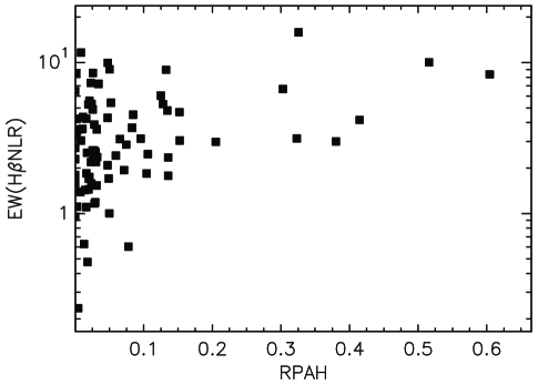
Figure 17: Comparison between RPAH (PAH fraction from MIR data) with EW(H$\beta$NLR). Pearson’ correlation coefficient is $\rho$=0.38; P=0.00035.

The second eigenvector is dominated with MIR spectral index, $\alpha$ and EW([OIII]). $\alpha$ and EW(FeII) have positive projections, as well as $\rm S_{SIL}$ and log$\rm(L5100)$, but weaker. On the other hand, EW([OIII]), and consequently log([OIII]/H$\beta$NLR), have the negative projections. EW(H$\beta$NLR) is not projected on this eigenvector. This implies that as the $\alpha$ grows, the EW([OIII]) and log([OIII]/H$\beta$NLR) decreases, but EW(FeII) increases. In this eigenvector is projected the anticorrelation between EW([OIII]) and EW(FeII) from BG92 EV1, which seems to be related with $\alpha$.

The third eigenvector is dominated by EW($\rm H\beta_{broad}$), which correlates with the FWHM(H$\beta$) broad line and anticorrelates with EWs of the narrow lines.

The fourth eigenvector is strongly dominated with the strength of the silicate feature ($\rm S_{SIL}$) which is correlated with FWHM(H$\beta$). This implies the connection between the widths of the broad lines and inclination angle or geometry of torus.

5 Discussion

5.1 BPT diagram at MIR wavelengths

In the Section 4.4, we found a certain disagreement between optical and MIR quantifying of the SB contribution to the AGN spectra, for both the Type 1 and Type 2 AGNs. The presence of the Type 1 AGNs on the SB part of the BPT diagram that we noticed here is earlier observed (Popović et al., 2009; Popović & Kovačević, 2011; Wang et al., 2006).

We do not completely understand the reason of the misplacement of these objects on the BPT diagram. The extinction at the optical wavelengths is one of the most often explanations, although some authors believe that the radiation may come from the different regions and/or that the slit difference between SDSS and IRS might contribute to this disagreement (Vika et al., 2017). We can not exclude the possibility of the imperfection of some of the methods, such as the decomposition or fitting. These results remind to the results of Goulding & Alexander (2009) and Dixon & Joseph (2011), who found that there may exist AGNs in half of the luminous IR galaxies without any evidence of AGN at the near-infrared and optical wavelengths.

It seems that the Type 1 AGNs have a lower disagreement than the Type 2. The possible reasons for that are: 1) Maybe since the AGN signature is more prominent in the Type 1 sample; 2) The column density should be lower for the Type 1 than for Type 2 AGNs, thus the probability to observe the different regions of the AGN in optical and MIR is lower; 3) Because the Type 1 sample is more homogeneous and may be more accurate.

Another cause of this disagreement between optical and MIR SB/AGN dominance could be the difference in the emission from within the optical or MIR wavebands sampled by the data. The only way to properly estimate which power source dominates the emission in galaxy is to sample the full SED or to apply bolometric corrections to the data. Methods of this type have been done in analyses of ULIRGs from various groups (Veilleux et al., 2009; Armus et al., 2007; Petric et al., 2007).

5.2 Comparison between the optical and MIR SB/AGN diagnostics

As we mentioned, the objects with R$<$0.5 have somewhat different certain optical characteristics (Popović & Kovačević, 2011; Kovačević-Dojčinović & Popović, 2015); which is believed to be caused by SB presence. However, as we obtained, on Fig. 16, objects with R$<$0.5 do not always have a high RPAH contribution, therefore there may exist some other reason why these objects have special optical characteristics.

PCA of the optical and MIR parameters confirms the results of BG92 and the other authors. It shows that R is probably influenced by more different physical properties of AGNs. Namely, EW($\rm H\beta$NLR) is correlated with SB strength in MIR, while [OIII] lines are correlated with $\alpha$. This means that R is indeed influenced by the SB presence, but also influenced by some other physical property which affects $\alpha$, which may be the cause of disagreement between MIR and optical diagnostics of the SB presence.

5.3 Connection between BG92 EV1 and MIR properties

Since BG92 established the set of correlations between AGN Type 1 spectral properties (EV1 in their PCA), it has been many attempts to explain their physical origin. The most frequently proposed governing mechanisms are: 1) Eddington ratio, L/$\rm L_{edd}$ (Boroson, 2002; Grupe, 2004) 2) AGN orientation (Bisogni et al., 2017), 3) and combination of these two properties (Marziani et al., 2001; Shen & Ho, 2014).

It was proposed that BG92 EV1 correlations can be considered as a surrogate "H–R Diagram" for Type 1 AGNs, with a main sequence driven by Eddington ratio convolved with line-of-sight orientation (Sulentic et al., 2000; Shen & Ho, 2014), for a review see Sulentic & Marziani (2015). Also, the BG92 EV1 is considered as an indicator of the AGN evolution (Marziani et al., 2003; Grupe, 2004; Wang et al., 2006; Popović & Kovačević, 2011). The evolution of AGNs is probably related with SB regions, assuming that there is stronger presence of the SB nearby the central engine of AGN in an earlier phase of AGN evolution, while in the later phases, the SB contribution probably becomes weaker and/or negligible (Hopkins et al., 2005; Lipari & Tarlevich, 2006; Wang & Wei, 2008; Sani et al., 2010).

To understand the physical background of BG92 EV1 correlations, in Section 4.5, we performed PCA using several optical and MIR spectral parameters. When interpreting the PCA results, it is important to take into account that an eigenvector is always specific to a certain sample, depending which observed parameters have been used and on the range of the parameters (Grupe, 2004). Therefore, each individual sample has its own eigenvectors, e.g. when using a set of different spectral parameters for PCA, BG92 EV1 can be projected on some other eigenvector, or divided into two or more eigenvectors. In this analysis, RPAH is chosen as a SB indicator (see Peeters et al., 2004; Brandl et al., 2006; Houck et al., 2007), $\alpha$ as a MIR spectral index of the pure AGN continuum, and $\rm S_{SIL}$ should be an indicator of the geometry and inclination (Hao et al., 2007). The results of the PCA are summarized in Table 8, where correlations between the optical and MIR parameters are denoted with uprising arrows, anti-correlations with decreasing arrows, and lack of any connection (projections to eigenvectors$<$0.25) with zero. In cases of weak connection (0.25$<$projections to eigenvector$<$0.30) we note "weak" in Table 8. These results imply that the two the most interesting BG92 EV1 anti-correlations (EW(FeII) vs. FWHM(H$\beta$) and EW(FeII) vs. EW([OIII])) are related with different MIR parameters, since they are projected into two different eigenvectors in our analysis. The first dominated with RPAH and the second with $\alpha$. The EW(FeII) vs. FWHM(H$\beta$) anti-correlation is connected with SB presence (RPAH), while EW(FeII) vs. EW([OIII]) seems to be connected with some physical property, reflected in $\alpha$. The $\alpha$ is a complex parameter which reflects MIR SED, and therefore depends on several physical properties as: i) accretion disc radiation (which depends on Eddington ratio, L/$\rm L_{edd}$, (see Zhang et al., 2008), ii) inclination, and iii) torus physical properties as geometry, dust distribution, optical depth, etc. (Stalevski et al., 2012).

Table 8: The summary of the PCA performed in the Section 4.5 and discussed in Sections 5.2 and 5.3.

	RPAH	$\alpha$	$\rm S_{SIL}$
	EV1	EV2	EV3
EW([OIII])	0	$\searrow$	0
EW(FeII)	$\nearrow$	$\nearrow$	0
EW(H$\beta$NLR)	$\nearrow$	0	$\nearrow$
EW(H$\beta$Broad)	0	0	$\nearrow$ weak
log(OIII5007/H$\beta$NLR)	$\searrow$	$\searrow$	0
FWHM(H$\beta$)	$\searrow$	0	$\nearrow$
log(L5100)	$\searrow$	$\nearrow$ weak	0

Although it is supposed that they are dominantly driven by different physical properties, the relation between RPAH, $\alpha$ and $\rm S_{SIL}$ seems to be complex. Hernán-Caballero et al. (2015) tested the validity of the MIR spectral decomposition of deblendIRS code (see their Section 3.2), and found that $\alpha$ is in significant correlation with nuclear spectral index derived from ground-based observations. Although $\alpha$ should be a pure AGN property, it is in a weak anticorrelation with the RPAH, EWPAH7.7 and EWPAH11.2 in our sample (see Table 6). The trend between $\alpha$ and RPAH may be caused by the reverse dependence between RPAH and RAGN (see Fig. 6). The trend between the $\alpha$ and EW of PAHs is probably present because EWs are measured relative to the total continuum flux, with AGN flux included. We found a weak trend between $\alpha$ and $\rm S_{SIL}$ in our correlation matrix (Table 6) and Section 4.1 (as noticed by Hao et al., 2007; Hernán-Caballero et al., 2015).

Wang et al. (2006) used the MIR color $\alpha$(60,25) as an indicator of the SB presence, and found its correlation with BG92 EV1 correlations. Note, that the MIR color $\alpha$(60,25) is measured using the total (AGN+SB) flux, and therefore it contains information about the SB presence and AGN continuum slope, which are in this work separated in two parameters, RPAH and $\alpha$. Our results are consistent with results of Wang et al. (2006), but we give more detailed insight in origin of BG92 EV1 correlations.

6 Conclusions

Here we investigate the optical and MIR spectral properties of a sample of 82 Type 1 AGNs. Additionally, to check the results based on the narrow lines (which are superposed with broad lines in the Type 1 AGNs), we considered a sample of 49 Type 2 AGNs. We carefully fit the optical spectra using methods described in Popović et al. (2004), Kovačević et al. (2010) and Kovačević-Dojčinović & Popović (2015). For fitting of MIR data we used deblendIRS code described in Hernán-Caballero et al. (2015). Concerning our investigation, we can outline following conclusions:

1. In sample of Type 1, we see more silicate emission, than absorption, which is expected, according to Hao et al. (2007); Stalevski et al. (2011) and Weedman et al. (2012).

2. We did not find any linear trend in the correlation matrix between EW(PAH) or RPAH with FWHM(H$\beta$) (see Table 6), but PCA shows anticorrelation between these properties, which is in an agreement with the result of Sani et al. (2010), who found that the narrower broad FWHM(H$\beta$) have stronger a PAH emission.

3. The separation between AGN and SB based on the BPT diagram does not give the same result as the one from MIR spectra in both Type 1 and Type 2 AGN samples. Some of the possible reasons are extinction at optical wavelengths (Dixon & Joseph, 2011), different sizes of slits, or the radiation may come from the different regions (Vika et al., 2017).

4. The weak correlation between the main optical (log([OIII]5007/H$\beta$NLR)) and MIR (RPAH) starburst estimators implies that the difference in the optical characteristics in the objects with log([OIII]5007/H$\beta$NLR)$<$0.5 and $>$0.5 (Popović & Kovačević, 2011; Kovačević-Dojčinović & Popović, 2015) may have a different reason than the star formation presence.

5. PCA shows that the anticorrelations between EW(FeII) vs. FWHM(H$\beta$), as well as EW(FeII) vs. EW([OIII]), from BG92 EV1, probably have a different governing mechanism: the former is connected with SB presence, while the latter is more connected with the MIR AGN spectral index.

6. PCA implies that the ratio log([OIII]5007/H$\beta$NLR) is indeed influenced by the starburst presence, but also influenced by some other physical property (MIR AGN spectral index), which may be the cause of disagreement between MIR and optical diagnostics of the starburst presence in AGN spectra.

7. A well known AGN indicator, EW([OIII]) is related to the MIR spectral index $\alpha$, but not related to the AGN or PAH fraction.

8. Since the BPT and MIR SB/AGN diagnostics do not necessarily trace the contribution of an AGN to the total power of the galaxy, the dissagrement between the two methods is not overly unexpected.

Finally, here we confirm some correlations between the optical and IR spectral properties that have been governed by presence of the SB contribution. EW(FeII) and EW(H$\beta$NLR) are correlated with RPAH. Anticorrelation EW(FeII) vs. FWHM(H$\beta$) may be also connected with the RPAH, since they are projected on the same eigenvector as RPAH.

Appendix A Estimation of the narrow emission lines for the BPT diagram

The axes in the BPT diagram are the ratios of the particular narrow lines ([OIII]/H$\beta$NLR and [NII]/H$\alpha$NLR) and therefore the accurate measurements of the fluxes of these lines is very important for correct AGN/SB diagnostics.

In the Type 1 AGNs, these narrow lines overlap with the broad lines, and in some cases it is very difficult to distinguish them. We use the same fitting procedure as in Popović & Kovačević (2011), where the confidence of the narrow H$\beta$ component estimation and non-uniqueness in the solutions is tested and discussed (see Appendix A in Popović & Kovačević, 2011).

As it is explained in Section 3.1.2, we use the same parameters for widths and shifts for all considered narrow lines ([OIII], H$\beta$NLR, [NII] and H$\alpha$NLR). In this way, we are getting less degree of freedom in the fitting procedure and more confident fits in the case when one of these lines can not be distinguished well from the broad lines.

In our sub-sample of 69 objects with available optical range of $\lambda\lambda$6200-6950Å (which covers [NII] and H$\alpha$), in 26 objects [NII] lines are are very weak and barely seen in the broad H$\alpha$ profiles. These objects are assigned in the BPT diagram as less confident (empty squares, see Fig. 14). The example of this kind of objects is shown in Fig. 18. On the other hand, in 43 objects from the sub-sample, [NII] lines can be well resolved from the broad H$\alpha$ profile (see the example in Fig. 19), and these object are assigned in the BPT diagram as more confident (full squares in Fig. 14).

Figure 18: An example of the fit of object (SDSS J130947.00$+$081948.24) with weak [NII] lines, which are difficult to be resolved in the broad H$\alpha$ profile.

Figure 19: An example of the fit of object (SDSS J135406.43$+$232549.40) with the strong and prominent [NII] lines.

References

- Alam et al. (2015) Alam, S., Albareti, F. D., Allende, P., et al. 2015, ApJS, 219, 12A
- Alonso-Herrero et al. (2014) Alonso-Herrero, A., Ramos Almeida, C., Esquej, P., et al. 2014, MNRAS, 443, 2766
- Armus et al. (2007) Armus, L., Charmandaris, V., Bernard-Salas, J., et al. 2007, ApJ, 656, 148A
- Baldwin et al. (1981) Baldwin, J. A., Phillips, M. M., & Terlevich, R. 1981, PASP, 93, 5
- Barvainis et al. (1987) Barvainis, R. 1987, ApJ, 320, 537
- Bian et al. (2016) Bian, W.-H., He, Z.-C., Green, G., Shi, Y., Ge, X., Liu, W.-S. 2016, MNRAS, 456, 4081
- Bisogni et al. (2017) Bisogni, S., Marconi, A., Risaliti, G. 2017, MNRAS, 464, 385
- Bon et al. (2006) Bon, E., Popović, L. Č., Ilić, D. & Mediavilla, E. G. 2006, New Astronomy Reviews, 50, 716
- Bon et al. (2009) Bon, E., Popović, L. Č., Gavrilović, N., La Mura, G. & Mediavilla, E. G. 2009, MNRAS, 400, 924
- Bonfield et al. (2011) Bonfield, D. G., Jarvis, M. J., Hardcastle, M. J., et al. 2011, MNRAS, 416, 13
- Boroson & Green (1992) Boroson, T. A. & Green, R. F. 1992, ApJS, 80, 109
- Boroson (2002) Boroson, T. A. 2002, ApJ, 565, 78
- Brandl et al. (2006) Brandl, B. R., Bernard-Salas, J., Spoon, H. W. W. et al. 2006, ApJ, 653, 1129
- Calzetti et al. (2000) Calzetti, D., Armus, L., Bohlin, R. C., Kinney, A. L., Koornneef, J., & Storchi-Bergmann, T. 2000, ApJ, 533, 682
- Chen & Shan (2014) Chen, P. S., & Shan, H. G. 2014, MNRAS, 441, 513
- Clavel et al. (2000) Clavel, J., Schulz, B., Altieri, B., et al. 2000, A&A, 357, 839
- Connolly et al. (1995) Connolly, A. J., Szalay, A. S., Bershady, M. A., Kinney, A. L., & Calzetti, D. 1995, AJ, 110, 1071
- Croton et al. (2006) Croton, D. J., Springel, V., Whiteet, S. D. M., et al. 2006, MNRAS, 365, 11
- Contini (2016) Contini, M. 2016, MNRAS, 461, 2374
- Deo et al. (2007) Deo, R. P., Crenshaw, D. M., Kraemer, S. B., Dietrich, M., Elitzur, M., Teplitz, H., Turner, T. J., 2007, ApJ, 671,124
- Dimitrijević et al. (2007) Dimitrijević, M. S., Popović, L. Č., Kovačević, J., Dačić, M., Ilić, D. 2007, MNRAS, 374, 1181
- Dixon & Joseph (2011) Dixon, T. G., & Joseph, R. D. 2011, ApJ, 740, 99
- Dong et al. (2008) Dong, X., Wang, T., Wang, J., Yuan, W., Zhou, H., Dai, H., & Zhang, K. 2008, MNRAS, 383, 581
- Feltre et al. (2013) Feltre, A., Hatziminaoglou, E., Hernán-Caballero, et al. 2013, MNRAS, 434, 2426
- Feng et al. (2014) Feng, H., Shen, Y., & Li, H. 2014, ApJ, 794, 77
- Feng et al. (2015a) Feng, Q.-C., Wang, J., Li, H.-L., & Wei, J.-Y. 2015a, Research in Astronomy and Astrophysics, 15, 199F
- Feng et al. (2015b) Feng, Q.-C., Wang, J., Li, H.-L., & Wei, J.-Y. 2015b, Research in Astronomy and Astrophysics, 15, 663F
- Förster Schreiber et al. (2004) Förster Schreiber, N. M., Roussel, H., Sauvage, M., & Charmandaris, V., 2004, A&A, 419, 501
- Francis et al. (1992) Francis, P. J., Hewett, P. C., Foltz, C. B., Chaffee, F. H. 1992, ApJ, 389, 476
- García-Bernete et al. (2016) García-Bernete, I., Ramos Almeida, C., Acosta-Pulido, J. A., et al. 2016, MNRAS, 463,3531
- Gaskell (2017) Gaskell, C. M. 2017, MNRAS, 467, 226
- Genzel et al. (1998) Genzel, R., Lutz, D., Sturm, E., et al. 1998, ApJ, 498, 579
- Goulding & Alexander (2009) Goulding, A. D. & Alexander, D. M. 2009, MNRAS, 398, 1165
- Grupe (2004) Grupe, D., 2004, AJ, 127, 1799
- Haas et al. (2007) Haas, M., Siebenmorgen, R., Pantin, E., Horst, H., Smette, A., Käufl, H.-U., Lagage, P.-O., & Chini, R., 2007, A&A, 473, 369
- Hao et al. (2007) Hao, L., Weedman, D. W., Spoon, H. W. W., Marshall, J. A., Levenson, N. A., Elitzur, M., Houck, J. R. 2007, ApJ, 655, L77
- Hartigan et al. (2004) Hartigan, P., Raymond, J. & Pierson, R. 2004, ApJ, 614, L69
- Hernán-Caballero et al. (2015) Hernán-Caballero, A., Alonso-Herrero, A., Hatziminaoglou, E. et al. 2015, ApJ, 803, 109
- Hernán-Caballero et al. (2016) Hernán-Caballero, A., Spoon, H. W. W., Lebouteiller, V., Rupke, D. S. N. & Barry, D. P. 2016, MNRAS, 445, 1796
- Ho et al. (1997) Ho, L. C., Filippenko, A. V. & Sargent, W. L. 1997, ApJS, 112, 315
- Hopkins et al. (2005) Hopkins, P. F., Hernquist, L., Cox, T. J., Di Matteo, T., Martini, P., Robertson, B., Springel, V. 2005, ApJ, 630, 705
- Houck et al. (2004) Houck, J. R., Roellig, T. L., van Cleve, J., et al. 2004, ApJS, 154, 18
- Houck et al. (2007) Houck, J. R., Weedman, D. W., LeFloch, E., Hao, L. 2007, ApJ, 671, 323
- Howarth & Murray (1987) Howarth, I. D. & Murray, J. M. 1987, SERC STARLINK User note No. 50
- Howarth (1983) Howarth, I. D. 1983, MNRAS, 203, 301
- Hu et al. (2008) Hu, C., Wang, J.-M., Chen, Y.-M., Bian, W. H., Xue, S. J. 2008, ApJ, 683, 115
- Ilić et al (2012) Ilić, D., Popović, L. Č, La Mura, G., Ciroi, S., & Rafanelli, P. 2012, A&A, 543A, 142
- Ishibashi & Fabian (2016) Ishibashi, W. & Fabian, A. C. 2016, MNRAS, 463, 1291
- Kauffmann et al. (2003) Kauffmann, G., Heckman, T. M., Tremonti, C., et al. 2003, MNRAS, 346, 1055
- Kewley et al. (2001) Kewley, L. J., Dopita, M. A., Sutherland, R. S., Heisler, C. A., Trevena, J. 2001, ApJ, 556, 121
- Kirkpatrick et al. (2015) Kirkpatrick, A., Pope, A., Sajina, A., et al. 2015, ApJ, 814, 9
- Kovačević et al. (2010) Kovačević, J., Popović, L. Č. & Dimitrijević, M., 2010, ApJS, 189,15
- Kovačević-Dojčinović & Popović (2015) Kovačević-Dojčinović, J., Popović, L. Č. 2015, ApJS, 221,35
- Kuraszkiewicz et al. (2002) Kuraszkiewicz, J. K., Green, P. J., Forster, K., Aldcroft, T. L., Evans, I. N. & Koratkar, A. 2002, ApJS, 143, 257
- Lacy et al. (2013) Lacy, M., Ridgway, S. E., Gates, E. L., et al. 2013, ApJS, 208, 24
- LaMassa et al. (2011) LaMassa, S. M., PhD thesis, The Johns Hopkins University, Uncovering hidden black holes: obscured AGN and their relationship to the host galaxy, 2011
- LaMassa et al. (2012) LaMassa, S. M., Heckman, T. M., Ptak, A., Schiminovich, D., O’Dowd, M., Bertincourt 2012, ApJ, 758, 1
- Laurent et al. (2000) Laurent, O., Mirabel, I. F., Charmandaris, V., et al. 2000, A&A, 359, 887
- Lebouteiller et al. (2011) Lebouteiller, V., Barry, D. J., Spoon, H. W. W., et al. 2011, ApJS, 196, 8
- Lebouteiller et al. (2010) Lebouteiller, V., Bernard-Salas, J., Sloan, G. C., & Barry, D. J. 2010, PASP, 122, 231
- Lipari & Tarlevich (2006) Lipari, S. L., & Terlevich, R. J. 2006, MNRAS, 368, 1001
- Lutz et al. (1998b) Lutz, D., Kunze, D., Spoon, H. W. W., and Thornley, M. D. 1998b, A&A333, 75
- Lutz et al. (2010) Lutz, D., Mainieri, V., Rafferty, D., et al. 2010, ApJ, 712, 1287
- Lutz et al. (1998a) Lutz, D., Spoon, H. W. W., Rigopoulou, D., Moorwood. A. F. M, Genzel. R. 1998a, ApJ505, 103
- Man et al. (2016) Man, A. W. S., Greve, T. R., Toft, S., et al. 2016, ApJ, 820, 1
- Mao et al. (2009) Mao, Y.-F., Wang, J., & Wei, J.-Y. 2009, RAA, 9, 529
- Marziani et al. (2003) Marziani, P. Zamanov, R. K., Sulentic, J. W., Calvani, M. 2003, MNRAS, 345, 1133
- Marziani et al. (2001) Marziani, P., Sulentic, J. W., Zwitter, T., Dultzin-Hacyan, D., Calvani, M. 2001, ApJ, 558, 553
- Melnick et al. (2015) Melnick, J., Telles, E., De Propris, R., & Chu, Z.-H. 2015, A&A, 582, A37
- O’Dowd et al. (2009) O’Dowd, M., Schiminovich, D., Johnson., B. D., et al. 2009, ApJ, 705, 885
- Peebles (1993) Peebles P.J.E. 1993, Principles of Physical Cosmology, Princeton University Press, Princeton
- Peeters et al. (2004) Peeters, E., Spoon, H. W. W., & Tielens, A. G. G. M. 2004, apj, 613, 986
- Petric et al. (2007) Petric, A. O., Lacy, M., Storrie-Lombardi, L., J., Sajina, A., Armus, L., Canalizo, G., & Ridgway, S. 2007, ASP Conf. Ser., 373, 497
- Popović (2003) Popović, L. Č. 2003, ApJ, 599, 140