Fully Finite Element Adaptive Algebraic Multigrid Method for Time-Space Caputo-Riesz Fractional Diffusion Equations

Abstract

The paper aims to establish a fully discrete finite element (FE) scheme and provide cost-effective solutions for one-dimensional time-space Caputo-Riesz fractional diffusion equations on a bounded domain $\Omega$. Firstly, we construct a fully discrete scheme of the linear FE method in both temporal and spatial directions, derive many characterizations on the coefficient matrix and numerically verify that the fully FE approximation possesses the saturation error order under $L^{2}(\Omega)$ norm. Secondly, we theoretically prove the estimation $1+\mathcal{O}(\tau^{\alpha}h^{-2\beta})$ on the condition number of the coefficient matrix, in which $\tau$ and $h$ respectively denote time and space step sizes. Finally, on the grounds of the estimation and fast Fourier transform, we develop and analyze an adaptive algebraic multigrid (AMG) method with low algorithmic complexity, reveal a reference formula to measure the strength-of-connection tolerance which severely affect the robustness of AMG methods in handling fractional diffusion equations, and illustrate the well robustness and high efficiency of the proposed algorithm compared with the classical AMG, conjugate gradient and Jacobi iterative methods.

1 Introduction

In recent years, there has been an explosion of research interest in numerical solutions for fractional differential equations, mainly due to the following two aspects: (i) the huge majority can’t be solved analytically, (ii) the analytical solution (if luckily derived) always involve certain infinite series which sharply drives up the costs of its evaluation. Various numerical methods have been proposed to approximate more accurately and faster, such as finite difference (FD) method [1, 2, 3, 4, 5, 6, 7, 8, 9, 10], finite element (FE) method [11, 12, 13, 14, 15, 16, 17], finite volume [18] method and spectral (element) method [19, 20, 21, 22, 23, 24, 25]. An essential challenge against standard differential equations lies in the presence of the fractional differential operator, which gives rise to nonlocality (space fractional, nearly dense or full coefficient matrix) or memory-requirement (time fractional, the entire time history of evaluations) issue, resulting in a vast computational cost.

Preconditioned Krylov subspace methods are regarded as one of the potential solutions to the aforementioned challenge. Numerous preconditioners with various Krylov-subspace methods have been constructed respectively for one- and two-dimensional, linear and nonlinear space-fractional diffusion equations (SFDE) [26, 27, 28, 29, 30]. Multigrid method has been proven to be a superior solver and preconditioner for ill-conditioned Toeplitz systems as well as SFDE. Pang and Sun propose an efficient and robust geometric multigrid (GMG) with fast Fourier transform (FFT) for one-dimensional SFDE by an implicit FD scheme [31]. Bu et al. employ the GMG to one-dimensional multi-term time-fractional advection-diffusion equations via a fully discrete scheme by FD method in temporal and FE method in spatial directions [32]. Jiang and Xu construct optimal GMG for two-dimensional SFDE to get FE approximations [33]. Chen et al. make the first attempt to present an algebraic multigrid (AMG) method with line smoothers to the fractional Laplacian through localizing it into a nonuniform elliptic equation [34]. Zhao et al. invoke GMG for one-dimensional Riesz SFDE by an adaptive FE scheme using hierarchical matrices [35]. From the survey of references, in spite of quite a number of contributions to numerical methods and preconditioners, there are no calculations taking into account of fully discrete FE schemes and AMG methods for time-space Caputo-Riesz fractional diffusion equations.

In this paper, we are concerned with the following time-space Caputo-Riesz fractional diffusion equation (CR-FDE)

$${}_{0}^{C}D^{\alpha}_{t}u(x,t)=\frac{\partial^{2\beta}u(x,t)}{\partial|x|^{2\beta}}+f(x,t),~{}~{}t\in I=(0,T],~{}x\in\Omega=(a,b)$$ (1)

$$u(x,t)=0,~{}~{}t\in I,~{}x\in\partial\Omega$$ (2)

$$u(x,0)=\psi_{0}(x),~{}~{}x\in\Omega$$ (3)

with orders $\alpha\in(0,1)$ and $\beta\in(1/2,1)$, the Caputo and Riesz fractional derivatives are respectively defined by

$${}_{0}^{C}D^{\alpha}_{t}u=\frac{1}{\Gamma(1-\alpha)}\int_{0}^{t}(t-s)^{-\alpha}\frac{\partial u}{\partial s}ds,~{}\frac{\partial^{2\beta}u}{\partial|x|^{2\beta}}=-\frac{1}{2\cos(\beta\pi)}({}_{x}D_{L}^{2\beta}u+{}_{x}D_{R}^{2\beta}u),$$

where

$${}_{x}D_{L}^{2\beta}u=\frac{1}{\Gamma(2-2\beta)}\frac{\partial^{2}}{\partial x^{2}}\int_{a}^{x}(x-s)^{1-2\beta}uds,~{}{}_{x}D_{R}^{2\beta}u=\frac{1}{\Gamma(2-2\beta)}\frac{\partial^{2}}{\partial x^{2}}\int_{x}^{b}(s-x)^{1-2\beta}uds.$$

The remainder of this paper proceeds as follows. A fully discrete FE method of (1)-(3) is developed in Section 2. Section 3 comes up with the theoretical estimation and verification experiments on the condition number of the coefficient matrix. The classical AMG method is introduced in Section 4 followed by its uniform convergence analysis and the construction of an adaptive AMG method. Section 5 reports and analyzes numerical results to show the benefits. We close in Section 6 with some concluding remarks.

2 Fully discrete finite element scheme for the CR-FDE

For simplicity, following [36], we will use the symbols $\lesssim$, $\gtrsim$ and $\simeq$ throughout the paper. $u_{1}\lesssim v_{1}$ means $u_{1}\leq C_{1}v_{1}$, $u_{2}\gtrsim v_{2}$ means $u_{2}\geq c_{2}v_{2}$ while $u_{3}\simeq v_{3}$ means $c_{3}v_{3}\leq u_{3}\leq C_{3}v_{3}$, where $C_{1}$, $c_{2}$, $c_{3}$ and $C_{3}$ are generic positive constants independent of variables, time and space step sizes.

2.1 Reminder about fractional calculus

In this subsection, we briefly introduce some fractional derivative spaces and several auxiliary results. Here the $L^{2}$ inner product and norm are denoted by

$$(u,v)_{L^{2}(\Omega)}=\int_{\Omega}uvdx,~{}\|u\|_{L^{2}(\Omega)}=(u,u)^{\frac{1}{2}}_{L^{2}(\Omega)}.$$

Definition 1

(Left and right fractional derivative spaces) For constant $\mu>0$, define norms

$$\|u\|_{J_{L}^{\mu}(\Omega)}:=(\|u\|^{2}_{L^{2}(\Omega)}+\|{}_{x}D_{L}^{\mu}u\|^{2}_{L^{2}(\Omega)})^{\frac{1}{2}},~{}\|u\|_{J_{R}^{\mu}(\Omega)}:=(\|u\|^{2}_{L^{2}(\Omega)}+\|{}_{x}D_{R}^{\mu}u\|^{2}_{L^{2}(\Omega)})^{\frac{1}{2}},$$

and let $J_{L,0}^{\mu}(\Omega)$ and $J_{R,0}^{\mu}(\Omega)$ be closures of $C_{0}^{\infty}(\Omega)$ under $\|\cdot\|_{J_{L}^{\mu}(\Omega)}$ and $\|\cdot\|_{J_{R}^{\mu}(\Omega)}$, respectively.

Definition 2

(Fractional Sobolev space) For constant $\mu>0$, define the norm

$$\|u\|_{H^{\mu}(\Omega)}:=(\|u\|^{2}_{L^{2}(\Omega)}+\||\xi|^{\mu}\tilde{u}\|^{2}_{L^{2}(\Omega_{\xi})})^{\frac{1}{2}},$$ (4)

and let $H_{0}^{\mu}(\Omega)$ be the closure of $C_{0}^{\infty}(\Omega)$ under $\|\cdot\|_{H^{\mu}(\Omega)}$, where $\tilde{u}$ is the Fourier transform of $u$.

Remark 1

The equivalence between (4) and the general definition of the norm has been established in [14], which implies the reasonability of Definition 2.

Lemma 1

(see [12], Proposition 1) If constant $\mu\in(0,1)$, $u,v\in J_{L,0}^{2\mu}(\Omega)$ (or $J_{R,0}^{2\mu}(\Omega)$), then

$$({}_{x}D_{L}^{2\mu}u,v)_{L^{2}(\Omega)}=({}_{x}D_{L}^{\mu}u,{}_{x}D_{R}^{\mu}v)_{L^{2}(\Omega)},~{}({}_{x}D_{R}^{2\mu}u,v)_{L^{2}(\Omega)}=({}_{x}D_{R}^{\mu}u,{}_{x}D_{L}^{\mu}v)_{L^{2}(\Omega)}.$$

Lemma 2

(see [11], Lemma 2.4) For constant $\mu>0$, we have

$$({}_{x}D_{L}^{\mu}u,{}_{x}D_{R}^{\mu}u)_{L^{2}(\Omega)}=\cos(\pi\mu)\|{}_{x}D_{L}^{\mu}u\|^{2}_{L^{2}(\Omega)}.$$ (5)

Lemma 3

(Fractional Poincaré-Friedrichs inequality, see [11], Theorem 2.10) For $u\in J_{L,0}^{\mu}(\Omega)$, we have

$$\|u\|_{L^{2}(\Omega)}\lesssim\|{}_{x}D_{L}^{\mu}u\|_{L^{2}(\Omega)}.$$ (6)

2.2 Derivation of the fully discrete scheme

By Lemma 1, we get the variational (weak) formulation of (1)-(3): given $f\in L^{2}(\Omega,I)$, $\phi_{0}\in L^{2}(\Omega)$ and $Q_{t}:=\Omega\times(0,t)$, to find $u\in\mathcal{H}$ subject to $u(x,0)=\psi_{0}(x)$ and

$$\Big{(}{}_{0}^{C}D^{\alpha}_{\sigma}u,v\Big{)}_{Q_{t}}+B^{t}_{\Omega}(u,v)=(f,v)_{Q_{t}},~{}\forall v\in\mathcal{H}^{*},$$ (7)

where $\mathcal{H}:=H_{0}^{\beta}(\Omega)\times H^{1}(I)$, $\mathcal{H}^{*}:=H_{0}^{\beta}(\Omega)\times L^{2}(I)$, and

$$\Big{(}{}_{0}^{C}D^{\alpha}_{\sigma}u,v\Big{)}_{Q_{t}}=\int_{0}^{t}\Big{(}{}_{0}^{C}D^{\alpha}_{\sigma}u,v\Big{)}_{L^{2}(\Omega)}d\sigma,~{}\Big{(}f,v\Big{)}_{Q_{t}}=\int_{0}^{t}\Big{(}f,v\Big{)}_{L^{2}(\Omega)}d\sigma,$$

$$B^{t}_{\Omega}(u,v)=\int_{0}^{t}\frac{1}{2\cos(\beta\pi)}\Big{[}({}_{x}D^{\beta}_{L}u,{}_{x}D^{\beta}_{R}v)_{L^{2}(\Omega)}+({}_{x}D^{\beta}_{R}u,{}_{x}D^{\beta}_{L}v)_{L^{2}(\Omega)}\Big{]}d\sigma.$$

In order to acquire numerical solutions of $u$, we firstly make a (possibly nonuniform) temporal discretization by points $0=t_{0}<t_{1}<\cdots<t_{N}=T$, and a uniform spatial discretization by points $x_{i}=a+ih$ ($i=0,1,\cdots,M$), where $h=(b-a)/M$ represents the space step size. Let

$$I_{j}=(t_{j-1},t_{j}),~{}\tilde{I}_{j}=(0,t_{j}),~{}j=1,2,\cdots,N;~{}\Omega_{h}=\{\Omega_{l}:\Omega_{l}=(x_{l-1},x_{l}),~{}l=1,2,\cdots,M\}.$$

We observe that it is convenient to form the FE spaces in tensor products

$$\mathcal{V}_{n}=\mathcal{V}^{\beta}_{h}(\Omega_{h})\times\mathcal{V}_{\tau}(\tilde{I}_{n}),~{}\mathcal{V}^{*}_{n}=\mathcal{V}^{\beta}_{h}(\Omega_{h})\times\mathcal{V}^{*}_{\tau}(I_{n}),$$

where

$$\mathcal{V}^{\beta}_{h}(\Omega_{h})=\{w_{h}\in H_{0}^{\beta}(\Omega)\cap C(\bar{\Omega}):~{}w_{h}(x)\big{|}_{\Omega_{l}}\in\mathcal{P}_{1}(\Omega_{l}),~{}l=1,\cdots,M\},$$

$$\mathcal{V}_{\tau}(\tilde{I}_{n})=\{v_{\tau}\in\mathcal{C}(\overline{\tilde{I}_{n}}):~{}v_{\tau}(0)=1,~{}v_{\tau}(t)\big{|}_{I_{j}}\in\mathcal{P}_{1}(I_{j}),~{}j=1,\cdots,n\},$$

$$\mathcal{V}^{*}_{\tau}(I_{n})=\{v_{\tau}\in L^{2}(I_{n}):~{}v_{\tau}(t)\big{|}_{I_{n}}\in\mathcal{P}_{0}(I_{n})\},$$

and $\mathcal{P}_{k}$ denotes the set of all polynomials of degree $\leq k$.

Remark 2

Apparently, for a given $u_{h\tau}(x,t)\in\mathcal{V}_{n}$, we have $\partial u_{h\tau}/\partial t\in\mathcal{V}^{*}_{n}$, where $\partial u_{h\tau}/\partial t$ is obtained by differentiating $u_{h\tau}$ with respect to $t$ on each subinterval $I_{j}$ ($j=1,2,\cdots,N$).

We obtain a fully discrete FE scheme in temporal and spatial directions of problem (7): given $Q_{n}:=\Omega_{h}\times I_{n}$, to find $u_{h\tau}\in\mathcal{V}_{n}$ such that $u_{h\tau}(x,0)=\psi_{0,I}(x)$ and

$$\Big{(}{}_{0}^{C}D^{\alpha}_{t}u_{h\tau},v_{h\tau}\Big{)}_{Q_{n}}+B^{n}_{\Omega}(u_{h\tau},v_{h\tau})=(f,v_{h\tau})_{Q_{n}},~{}\forall v_{h\tau}\in\mathcal{V}^{*}_{n},$$ (8)

where $\psi_{0,I}(x)\in\mathcal{V}_{n}$ satisfying $\psi_{0,I}(x_{i})=\psi_{0}(x_{i})$ ($i=0,1,\cdots,M$), and

$$\Big{(}{}_{0}^{C}D^{\alpha}_{t}u_{h\tau},v_{h\tau}\Big{)}_{Q_{n}}=\int_{t_{n-1}}^{t_{n}}({}_{0}^{C}D^{\alpha}_{t}u_{h\tau},v_{h\tau})_{L^{2}(\Omega)}dt,~{}(f,v_{h\tau})_{Q_{n}}=\int_{t_{n-1}}^{t_{n}}(f,v_{h\tau})_{L^{2}(\Omega)}dt,$$

$$B^{n}_{\Omega}(u_{h\tau},v_{h\tau})=\int_{t_{n-1}}^{t_{n}}\frac{1}{2\cos(\beta\pi)}\Big{[}({}_{x}D^{\beta}_{L}u_{h\tau},{}_{x}D^{\beta}_{R}v_{h\tau})_{L^{2}(\Omega)}+({}_{x}D^{\beta}_{R}u_{h\tau},{}_{x}D^{\beta}_{L}v_{h\tau})_{L^{2}(\Omega)}\Big{]}dt.$$

Let

$$\mathcal{L}_{0}(t)=\left\{\begin{aligned} &\frac{t_{1}-t}{\tau_{1}},~{}t\in I_{1}\\ &0,\qquad~{}t\in\tilde{I}_{n}\setminus I_{1}\end{aligned}\right.,~{}\tilde{\mathcal{L}}_{0}(t)=\frac{1}{\Gamma(1-\alpha)}\int_{t_{0}}^{t}\frac{d\mathcal{L}_{0}(s)}{(t-s)^{\alpha}},~{}\hat{\mathcal{L}}_{0}(t)=\frac{1}{\Gamma(1-\alpha)}\int_{t_{0}}^{t_{1}}\frac{d\mathcal{L}_{0}(s)}{(t-s)^{\alpha}},$$

$$\mathcal{L}_{k}(t)=\left\{\begin{aligned} &\frac{t_{k+1}-t}{\tau_{k+1}},~{}t\in I_{k+1}\\ &\frac{t-t_{k-1}}{\tau_{k}},~{}t\in I_{k}\\ &0,\qquad\quad~{}~{}t\in\tilde{I}_{n}\setminus(I_{k}\cup I_{k+1})\end{aligned}\right.,~{}\hat{\mathcal{L}}_{k}(t)=\frac{1}{\Gamma(1-\alpha)}\int_{t_{k-1}}^{t_{k+1}}\frac{d\mathcal{L}_{k}(s)}{(t-s)^{\alpha}},~{}k=1,\cdots,n-1$$

and

$$\mathcal{L}_{n}(t)=\left\{\begin{aligned} &\frac{t-t_{n-1}}{\tau_{n}},~{}t\in I_{n}\\ &0,\qquad\quad~{}~{}t\in\tilde{I}_{n}\setminus I_{n}\end{aligned}\right.,~{}\tilde{\mathcal{L}}_{n}(t)=\frac{1}{\Gamma(1-\alpha)}\int_{t_{n-1}}^{t}\frac{d\mathcal{L}_{n}(s)}{(t-s)^{\alpha}}.$$

Note that

$$\mathcal{V}^{*}_{n}=\textsf{span}\{\phi_{l}(x)\times 1,~{}l=1,\cdots,M-1\},$$

where $\phi_{l}(x)$ is the shape function at $x_{l}\in\Omega_{h}$. Using

$$u_{h\tau}(x,t)=u_{h}^{0}(x)\mathcal{L}_{0}(t)+\sum_{k=1}^{n-1}u_{h}^{k}(x)\mathcal{L}_{k}(t)+u_{h}^{n}(x)\mathcal{L}_{n}(t),$$

we have

$$({}_{0}^{C}D^{\alpha}_{t}u_{h\tau},\phi_{l}\times 1)_{Q_{1}}=(u_{h}^{0},\phi_{l})_{L^{2}(\Omega)}(\tilde{\mathcal{L}}_{0},1)_{L^{2}(I_{1})}+(u_{h}^{1},\phi_{l})_{L^{2}(\Omega)}(\tilde{\mathcal{L}}_{1},1)_{L^{2}(I_{1})},$$ (9)

$$({}_{0}^{C}D^{\alpha}_{t}u_{h\tau},\phi_{l}\times 1)_{Q_{n}}=(u_{h}^{0},\phi_{l})_{L^{2}(\Omega)}(\hat{\mathcal{L}}_{0},1)_{L^{2}(I_{n})}+$$

$$\qquad\sum_{k=1}^{n-1}(u_{h}^{k},\phi_{l})_{L^{2}(\Omega)}(\hat{\mathcal{L}}_{k},1)_{L^{2}(I_{n})}+(u_{h}^{n},\phi_{l})_{L^{2}(\Omega)}(\tilde{\mathcal{L}}_{n},1)_{L^{2}(I_{n})},~{}n>1,$$ (10)

$$\int_{t_{n-1}}^{t_{n}}1\times({}_{x}D^{\beta}_{L}u_{h\tau},{}_{x}D^{\beta}_{R}\phi_{l})_{L^{2}(\Omega)}dt=({}_{x}D^{\beta}_{L}u_{h}^{0},{}_{x}D^{\beta}_{R}\phi_{l})_{L^{2}(\Omega)}(\mathcal{L}_{0},1)_{L^{2}(I_{n})}+$$

$$\qquad\sum_{k=1}^{n-1}({}_{x}D^{\beta}_{L}u_{h}^{k},{}_{x}D^{\beta}_{R}\phi_{l})_{L^{2}(\Omega)}(\mathcal{L}_{k},1)_{L^{2}(I_{n})}+({}_{x}D^{\beta}_{L}u_{h}^{n},{}_{x}D^{\beta}_{R}\phi_{l})_{L^{2}(\Omega)}(\mathcal{L}_{n},1)_{L^{2}(I_{n})},$$ (11)

$$\int_{t_{n-1}}^{t_{n}}1\times({}_{x}D^{\beta}_{R}u_{h\tau},{}_{x}D^{\beta}_{L}\phi_{l})_{L^{2}(\Omega)}dt=({}_{x}D^{\beta}_{R}u_{h}^{0},{}_{x}D^{\beta}_{L}\phi_{l})_{L^{2}(\Omega)}(\mathcal{L}_{0},1)_{L^{2}(I_{n})}+$$

$$\qquad\sum_{k=1}^{n-1}({}_{x}D^{\beta}_{R}u_{h}^{k},{}_{x}D^{\beta}_{L}\phi_{l})_{L^{2}(\Omega)}(\mathcal{L}_{k},1)_{L^{2}(I_{n})}+({}_{x}D^{\beta}_{R}u_{h}^{n},{}_{x}D^{\beta}_{L}\phi_{l})_{L^{2}(\Omega)}(\mathcal{L}_{n},1)_{L^{2}(I_{n})}.$$ (12)

Substituting (9)-(2.2) into (8), yields

$$C^{n}_{h\tau}U^{n}_{h\tau}=G^{n}_{h\tau},$$ (13)

where the coefficient matrix

$$C^{n}_{h\tau}=M_{h}+\frac{\Gamma(3-\alpha)}{2}\tau^{\alpha}_{n}A_{h}^{\beta},$$ (14)

the right-hand side vector

$$G^{n}_{h\tau}=\Gamma(3-\alpha)\tau_{n}^{\alpha-1}F^{n}_{h\tau}+\Big{[}M_{h}-\frac{\Gamma(3-\alpha)}{2}\tau^{\alpha}_{n}A_{h}^{\beta}\Big{]}U^{n-1}_{h\tau}-\sum_{k=1}^{n-1}\tau_{n}^{\alpha-1}\times$$

$$\quad\frac{(t_{n}-t_{k-1})^{2-\alpha}-(t_{n-1}-t_{k-1})^{2-\alpha}-(t_{n}-t_{k})^{2-\alpha}+(t_{n-1}-t_{k})^{2-\alpha}}{\tau_{k}}M_{h}(U^{k}_{h\tau}-U^{k-1}_{h\tau}),$$

the mass matrix

$$M_{h}=\frac{h}{6}\left(\begin{array}[]{ccccc}4&1&&&\\ 1&4&1&&\\ &\ddots&\ddots&\ddots&\\ &&1&4&1\\ &&&1&4\end{array}\right)_{(M-1)\times(M-1)},$$ (20)

the stiffness matrix $A_{h}^{\beta}=(a^{h}_{i,j})_{(M-1)\times(M-1)}$ with its entries

$$\left\{\begin{aligned} &a^{h}_{i,i}=\frac{h^{1-2\beta}(2^{4-2\beta}-8)}{2\cos(\beta\pi)\Gamma(4-2\beta)},~{}~{}~{}\quad\qquad\qquad\qquad\qquad\qquad\qquad~{}~{}~{}~{}i=1,\cdots,M-1\\ &a^{h}_{j,j+1}=a^{h}_{j+1,j}=\frac{h^{1-2\beta}(3^{3-2\beta}-2^{5-2\beta}+7)}{2\cos(\beta\pi)\Gamma(4-2\beta)},~{}\quad\qquad\qquad\quad\quad j=1,\cdots,M-2\\ &a^{h}_{k,k+l}=a^{h}_{k+l,k}=\frac{h^{1-2\beta}}{2\cos(\beta\pi)\Gamma(4-2\beta)}[(l+2)^{3-2\beta}\\ &\quad\quad\quad-4(l+1)^{3-2\beta}+6l^{3-2\beta}-4(l-1)^{3-2\beta}+(l-2)^{3-2\beta}],~{}k=1,\cdots,M-l-1\end{aligned}\right.,$$ (21)

the vector

$$F^{n}_{h\tau}=(f^{n}_{1},f^{n}_{2},\cdots,f^{n}_{M-1})^{T},~{}f^{n}_{l}=(f,\phi_{l}\times 1)_{Q_{n}},~{}l=1,\cdots,M-1$$

and the fully FE approximations

$$U^{k}_{h\tau}=(u^{k}_{1},u^{k}_{2},\cdots,u^{k}_{M-1})^{T},~{}u^{0}_{j}=\psi_{0,I}(x_{j}),~{}u^{k}_{j}=u_{h}^{k}(x_{j}),~{}k=1,\cdots,n,~{}j=1,\cdots,M-1.$$

Remark 3

(13) is reduced via dividing both sides of (8) by the factor $\tau^{1-\alpha}_{n}/\Gamma(3-\alpha)$, in case of the severe loss in convergence of the fully discrete FE scheme.

Next, a number of characterizations are established regarding $A_{h}^{\beta}$ just defined by (21).

Theorem 1

The stiffness matrix $A_{h}^{\beta}$ is symmetric and satisfies

1. $a^{h}_{i,i}>0$ for $i=1,\cdots,M-1$;

2. $a^{h}_{i,j}<0$ for $i\neq j$, $i,j=1,\cdots,M-1$;

3. $\sum_{j=1}^{M-1}a^{h}_{i,j}>0$ for $i=1,\cdots,M-1$;

4. The following relation holds for the particular case when $h\leq 1/7$

   $$\sum\limits_{j=1}^{M-1}a^{h}_{i,j}\geq\left\{\begin{aligned} &-\frac{h^{1-2\beta}(4-2^{3-2\beta})}{2\cos(\beta\pi)\Gamma(4-2\beta)},~{}i=1,M-1\\ &-\frac{2^{2\beta}h(2\beta-1)}{\cos(\beta\pi)\Gamma(2-2\beta)},~{}~{}~{}i=2,\cdots,M-2\end{aligned}\right.;$$

5. $A_{h}^{\beta}$ is an M-matrix.

• The symmetric property of $A_{h}^{\beta}$ is an obvious fact by (21). Since $\beta\in(1/2,1)$, then $4-2\beta<3$ and $\cos(\beta\pi)<0$, which give immediately $a^{h}_{ii}>0$, $i=1,\cdots,M-1$. This proves the first part of the theorem. The second part is an immediate consequence of the facts that on the interval $\beta\in(1/2,1)$, $f(\beta)=3^{3-2\beta}-2^{5-2\beta}+7$ is a strictly increasing function, and the bivariate function

  $$f_{\beta}(l)=(l+2)^{3-2\beta}-4(l+1)^{3-2\beta}+6l^{3-2\beta}-4(l-1)^{3-2\beta}+(l-2)^{3-2\beta}>0,~{}2\leq l\leq M-2.$$

  In fact, it is evident that

  $$1.5^{2\beta}>1.5>\frac{3^{3}}{2^{5}}\frac{\ln 3}{\ln 2}\Rightarrow f^{\prime}(\beta)=-2\ln 3\cdot 3^{3-2\beta}+2\ln 2\cdot 2^{5-2\beta}>0,$$

  and

  $$f_{\beta}(l)=h^{2\beta-3}[g(x_{l+2})-4g(x_{l+1})+6g(x_{l})-4g(x_{l-1})+g(x_{l-2})]>0$$

  using Taylor’s expansion with

  $$(\frac{l}{l+1})^{2+2\beta}-(\frac{l}{l-1})^{2+2\beta}>-\frac{30l}{2\beta+1}\Rightarrow l^{-1-2\beta}+\frac{2\beta+1}{30}[{(l+1)}^{-2-2\beta}-{(l-1)}^{-2-2\beta}]>0,$$

  where $g(x)=(x-a)^{3-2\beta}$ and $x_{l}=lh+a$.

  To prove the third part, use

  $$({}_{x}D^{\beta}_{L}\phi_{i},{}_{x}D^{\beta}_{R}\phi_{j})_{L^{2}(\Omega)}=-({}_{x}D_{L}^{2\beta-1}\phi_{i},\frac{d\phi_{j}}{dx})_{L^{2}(\Omega)}$$

  and

  $$\tilde{\phi}:=\sum\limits_{j=1}^{M-1}\phi_{j}=1-\phi_{0}-\phi_{M}$$

  to obtain the relation

  $$\sum\limits_{j=1}^{M-1}a^{h}_{i,j}=-\frac{({}_{x}D_{L}^{2\beta-1}\tilde{\phi},1)_{\Omega_{i}}-({}_{x}D_{L}^{2\beta-1}\tilde{\phi},1)_{\Omega_{i+1}}+({}_{x}D_{L}^{2\beta-1}\phi_{i},1)_{\Omega_{1}}-({}_{x}D_{L}^{2\beta-1}\phi_{i},1)_{\Omega_{M_{h}}}}{2h\cos(\beta\pi)},$$

  where

  $${}_{x}D^{2\beta-1}_{L}\tilde{\phi}=\left\{\begin{aligned} &\frac{(x-a)^{2-2\beta}}{h\Gamma(3-2\beta)},~{}\qquad\qquad\qquad\qquad\qquad\qquad\qquad\quad~{}a<x<x_{1}\\ &\frac{(x-a)^{2-2\beta}-(x-x_{1})^{2-2\beta}}{h\Gamma(3-2\beta)},~{}\qquad\qquad\qquad\qquad~{}~{}x_{1}<x<x_{M_{h}-1}\\ &\frac{(x-a)^{2-2\beta}-(x-x_{1})^{2-2\beta}-(x-x_{M_{h}-1})^{2-2\beta}}{h\Gamma(3-2\beta)},~{}x_{M_{h}-1}<x<x_{M_{h}}\end{aligned}\right.$$

  and

  $${}_{x}D_{L}^{2\beta-1}\phi_{i}(x)=\left\{\begin{aligned} &0,\qquad\qquad\qquad\qquad\qquad\qquad\qquad\qquad\qquad\qquad\quad~{}x<x_{i-1}\\ &\frac{(x-x_{i-1})^{2-2\beta}}{h\Gamma(3-2\beta)},\qquad\qquad\qquad\qquad\qquad\qquad\qquad\quad x_{i-1}<x<x_{i}\\ &\frac{(x-x_{i-1})^{2-2\beta}-2(x-x_{i})^{2-2\beta}}{h\Gamma(3-2\beta)},\qquad\qquad\qquad\qquad x_{i}<x<x_{i+1}\\ &\frac{(x-x_{i-1})^{2-2\beta}-2(x-x_{i})^{2-2\beta}+(x-x_{i+1})^{2-2\beta}}{h\Gamma(3-2\beta)},~{}x>x_{i+1}\end{aligned}\right..$$

  Assume that $\Omega=(0,1)$ without loss of generality, one can easily derive

  $$\sum\limits_{j=1}^{M-1}a^{h}_{i,j}=-\frac{(4-2^{3-2\beta})h^{3-2\beta}-1+3(1-h)^{3-2\beta}-3(1-2h)^{3-2\beta}+(1-3h)^{3-2\beta}}{2\cos(\beta\pi)h^{2}\Gamma(4-2\beta)},~{}i=1,M-1,$$

  $$\sum\limits_{j=1}^{M-1}a^{h}_{i,j}=-\frac{3(ih)^{3-2\beta}-3[(i-1)h]^{3-2\beta}+[(i-2)h]^{3-2\beta}-[(i+1)h]^{3-2\beta}}{2\cos(\beta\pi)h^{2}\Gamma({4-2\beta})}$$

  $$-\frac{3(1-ih)^{3-2\beta}-[1-(i-1)h]^{3-2\beta}-3[1-(i+1)h]^{3-2\beta}+[1-(i+2)h]^{3-2\beta}}{2\cos(\beta\pi)h^{2}\Gamma({4-2\beta})},~{}i=2,\cdots,M-2$$

  and deduce $\sum_{j=1}^{M-1}a^{h}_{i,j}>0$ by Taylor’s formula and $\beta\in(1/2,1)$.

  Another step to do in the proof is the result 4, which follows from

  $$h\leq 1/7\Rightarrow 7-4(1-\xi)^{-1-2\beta}>-\frac{1}{\beta h}\Rightarrow-1+3(1-h)^{3-2\beta}-3(1-2h)^{3-2\beta}+(1-3h)^{3-2\beta}>0$$

  for all $\xi\in(0,2h)$,

  $$(\frac{i-1}{i})^{3+2\beta}>\frac{\beta+1}{21(\beta+1)+30i}\Rightarrow\frac{3(ih)^{3-2\beta}-3(ih-h)^{3-2\beta}+(ih-2h)^{3-2\beta}-(ih+h)^{3-2\beta}}{h^{3}(3-2\beta)(2-2\beta)(2\beta-1)(ih)^{-2\beta}}>1$$

  and

  $$\frac{3(1-ih)^{3-2\beta}-[1-(i-1)h]^{3-2\beta}-3[1-(i+1)h]^{3-2\beta}+[1-(i+2)h]^{3-2\beta}}{h^{3}(3-2\beta)(2-2\beta)(2\beta-1)(1-ih)^{-2\beta}}>1$$

  for $i=2,\cdots,M-2$, together with the inequality $(ih)^{-2\beta}+(1-ih)^{-2\beta}\geq 2^{1+2\beta}$.

  Finally, according to properties 1 and 2, the result 5 will be proved by showing that $(A_{h}^{\beta})^{-1}$ is nonnegative, which can be easily proved by contradiction with property 3.  

Observe from (20)-(21) that $M_{h}$ and $A_{h}^{\beta}$ are both symmetric Toeplitz matrices independent of any time terms. The under-mentioned corollaries are natural consequences of Theorem 1.

Corollary 1

The coefficient matrix $C^{n}_{h\tau}$ is a symmetric Toeplitz matrix. Furthermore, it will be independent of time level $n$ if the temporal discretization is also uniform.

Corollary 2

The coefficient matrix $C^{n}_{h\tau}$ is an M-matrix, if and only if

$$\frac{\tau_{n}^{\alpha}}{h^{2\beta}}>-\frac{2\cos(\beta\pi)\Gamma(4-2\beta)}{3\Gamma(3-\alpha)(3^{3-2\beta}-2^{5-2\beta}+7)}.$$ (22)

• This result will follow from Theorem 1, if we can show that

  $$\frac{h}{6}+\frac{\Gamma(3-\alpha)}{2}\tau^{\alpha}_{n}\frac{h^{1-2\beta}(3^{3-2\beta}-2^{5-2\beta}+7)}{2\cos(\beta\pi)\Gamma(4-2\beta)}<0,$$

  which is an immediate application of the condition (22).  

2.3 Numerical experiments and the saturation error order

Example 1

Consider (1)-(3) with $\Omega=(0,1)$, $T=1$, $\psi_{0}(x)=0$ and

$$f(x,t)=\frac{\Gamma(3-\alpha)}{\Gamma(3-2\alpha)}t^{2-2\alpha}x^{2}(1-x)^{2}+\frac{t^{2-\alpha}}{\cos(\beta\pi)}\Big{[}\frac{x^{2-2\beta}+(1-x)^{2-2\beta}}{\Gamma(3-2\beta)}-$$

$$~{}~{}~{}~{}~{}~{}~{}~{}~{}~{}~{}~{}~{}~{}~{}~{}~{}~{}~{}~{}~{}~{}~{}\frac{6x^{3-2\beta}+6(1-x)^{3-2\beta}}{\Gamma(4-2\beta)}+\frac{12x^{4-2\beta}+12(1-x)^{4-2\beta}}{\Gamma(5-2\beta)}\Big{]}.$$

The exact solution is $u(x,t)=t^{2-\alpha}x^{2}(1-x)^{2}$. In the case of uniform temporal and spatial meshes, Tables 1 and 2 present errors $\|e\|_{0}:=\|u(\cdot,1)-u_{h\tau}(\cdot,1)\|_{L^{2}(\Omega)}$ and convergence rates.

Table 1: Error results and convergence rates in spatial direction with $h=\tau$.

$N$	$\beta=0.6$						$\beta=0.8$
	$\alpha=0.01$		$\alpha=0.50$		$\alpha=0.99$		$\alpha=0.01$		$\alpha=0.50$		$\alpha=0.99$
	$\|e\|_{0}$	rate	$\|e\|_{0}$	rate	$\|e\|_{0}$	rate	$\|e\|_{0}$	rate	$\|e\|_{0}$	rate	$\|e\|_{0}$	rate
8	8.94E-4	-	8.78E-4	-	8.88E-4	-	9.73E-4	-	9.56E-4	-	9.72E-4	-
16	2.02E-4	2.15	1.98E-4	2.15	2.00E-4	2.15	2.34E-4	2.06	2.29E-4	2.06	2.33E-4	2.06
32	4.49E-5	2.17	4.42E-5	2.16	4.47E-5	2.16	5.51E-5	2.08	5.40E-5	2.08	5.49E-5	2.08
64	1.01E-5	2.15	1.00E-5	2.14	1.01E-5	2.14	1.30E-5	2.09	1.27E-5	2.09	1.29E-5	2.09
$N$	$\alpha=0.10$		$\alpha=0.25$		$\alpha=0.75$		$\alpha=0.10$		$\alpha=0.25$		$\alpha=0.75$
	$\|e\|_{0}$	rate	$\|e\|_{0}$	rate	$\|e\|_{0}$	rate	$\|e\|_{0}$	rate	$\|e\|_{0}$	rate	$\|e\|_{0}$	rate
8	8.90E-4	-	8.80E-4	-	8.83E-4	-	9.72E-4	-	9.63E-4	-	9.64E-4	-
16	1.99E-4	2.16	1.97E-4	2.16	1.99E-4	2.15	2.31E-4	2.07	2.28E-4	2.08	2.31E-4	2.06
32	4.39E-5	2.18	4.40E-5	2.16	4.44E-5	2.16	5.39E-5	2.10	5.34E-5	2.09	5.44E-5	2.09
64	9.95E-6	2.14	1.00E-5	2.14	1.01E-5	2.14	1.25E-5	2.11	1.26E-5	2.08	1.28E-5	2.09

Table 2: Error results and convergence rates in spatial direction with $h=\sqrt{\tau}$.

$N$	$\beta=0.6$						$\beta=0.8$
	$\alpha=0.01$		$\alpha=0.50$		$\alpha=0.99$		$\alpha=0.01$		$\alpha=0.50$		$\alpha=0.99$
	$\|e\|_{0}$	rate	$\|e\|_{0}$	rate	$\|e\|_{0}$	rate	$\|e\|_{0}$	rate	$\|e\|_{0}$	rate	$\|e\|_{0}$	rate
16	3.64E-3	-	3.63E-3	-	3.63E-3	-	3.76E-3	-	3.75E-3	-	3.75E-3	-
64	8.94E-4	1.01	8.87E-4	1.02	8.88E-4	1.02	9.73E-4	0.97	9.69E-4	0.98	9.72E-4	0.98
256	2.02E-4	1.07	2.00E-4	1.08	2.00E-4	1.08	2.34E-4	1.03	2.32E-4	1.03	2.33E-4	1.03
$N$	$\alpha=0.10$		$\alpha=0.25$		$\alpha=0.75$		$\alpha=0.10$		$\alpha=0.25$		$\alpha=0.75$
	$\|e\|_{0}$	rate	$\|e\|_{0}$	rate	$\|e\|_{0}$	rate	$\|e\|_{0}$	rate	$\|e\|_{0}$	rate	$\|e\|_{0}$	rate
16	3.64E-3	-	3.63E-3	-	3.63E-3	-	3.75E-3	-	3.75E-3	-	3.75E-3	-
64	8.90E-4	1.02	8.87E-4	1.02	8.86E-4	1.02	9.72E-4	0.98	9.71E-4	0.98	9.69E-4	0.98
256	2.01E-4	1.07	2.01E-4	1.07	2.00E-4	1.08	2.33E-4	1.03	2.33E-4	1.03	2.32E-4	1.03

From Tables 1 and 2, we can obtain that the fully FE solution $u_{h\tau}$ achieves the saturation error order $\mathcal{O}(\tau^{2}+h^{2})$ under $\|\cdot\|_{0}$ norm.

Fig. 1 illustrates the comparisons of exact solutions and numerical solutions of $\alpha=0.2$, $0.4$ and $\beta=0.6$, $0.8$ with $t=1$ and $h=\tau=1/32$.

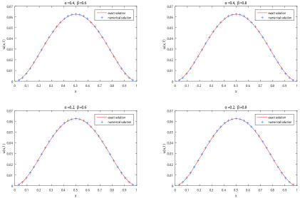
Figure 1: Illustration for comparisons on exact solutions and numerical solutions with $t=1$ and $h=\tau=1/32$.

3 Condition number estimation

This section is devoted to deriving the condition number estimation on the coefficient matrix of (13) in uniform temporal and and spatial discretizations.

Theorem 2

For the linear system (13), we have

$$\kappa(C^{n}_{h\tau})=1+\mathcal{O}(\tau^{\alpha}h^{-2\beta}).$$ (23)

• Let $C_{\alpha}=\Gamma(3-\alpha)/2$, we divide our proof in three steps. First, it is trivially true that $C^{n}_{h\tau}$ is spectrally equivalent to the matrix $I+C_{\alpha}\tau^{\alpha}M_{h}^{-\frac{1}{2}}A_{h}^{\beta}M_{h}^{-\frac{1}{2}}$, i.e.

  $$\kappa(C^{n}_{h\tau})\simeq\kappa\Big{(}I+C_{\alpha}\tau^{\alpha}M_{h}^{-\frac{1}{2}}A_{h}^{\beta}M_{h}^{-\frac{1}{2}}\Big{)}.$$ (24)

  The next thing to do in the proof is to verify

  $$\lambda_{\min}(M_{h}^{-\frac{1}{2}}A_{h}^{\beta}M_{h}^{-\frac{1}{2}})\gtrsim 1,~{}\lambda_{\max}(M_{h}^{-\frac{1}{2}}A_{h}^{\beta}M_{h}^{-\frac{1}{2}})\lesssim h^{-2\beta},$$ (25)

  which is equivalent to

  $$(\vec{v}_{h},\vec{v}_{h})\lesssim(M_{h}^{-\frac{1}{2}}A_{h}^{\beta}M_{h}^{-\frac{1}{2}}\vec{v}_{h},\vec{v}_{h})\lesssim h^{-2\beta}(\vec{v}_{h},\vec{v}_{h}),~{}\forall\vec{v}_{h}\in\mathbb{R}^{M-1}.$$ (26)

  Set $\vec{u}_{h}=M_{h}^{-\frac{1}{2}}\vec{v}_{h}:=(u^{h}_{1},\cdots,u^{h}_{M-1})^{T}$, rewrite (26) as $(M_{h}\vec{u}_{h},\vec{u}_{h})\lesssim(A_{h}^{\beta}\vec{u}_{h},\vec{u}_{h})\lesssim h^{-2\beta}(M_{h}\vec{u}_{h},\vec{u}_{h})$. It is sufficient to verify that $(M_{h}\vec{u}_{h},\vec{u}_{h})\simeq h(\vec{u}_{h},\vec{u}_{h})$. It follows by (20) and the Cauchy-Schwarz inequality that

  $$\frac{h}{3}(\vec{u}_{h},\vec{u}_{h})\leq(M_{h}\vec{u}_{h},\vec{u}_{h})=h\Big{[}\frac{2}{3}\sum_{l=1}^{M-1}(u^{h}_{l})^{2}+\frac{1}{3}\sum_{l=1}^{M-2}u^{h}_{l}u^{h}_{l+1}\Big{]}\leq h(\vec{u}_{h},\vec{u}_{h}).$$

  Thus (25) will follow if we can show that $h(\vec{u}_{h},\vec{u}_{h})\lesssim(A_{h}^{\beta}\vec{u}_{h},\vec{u}_{h})\lesssim h^{1-2\beta}(\vec{u}_{h},\vec{u}_{h}).$ We start by showing the second inequality. Utilizing Theorem 1 and the Cauchy-Schwarz inequality, we arrive at

  $$(A_{h}^{\beta}\vec{u}_{h},\vec{u}_{h}) \leq \sum_{i=1}^{M-1}a^{h}_{i,i}(u^{h}_{i})^{2}-\frac{1}{2}\sum_{i=1}^{M-1}\sum_{j\neq i}a^{h}_{i,j}[(u^{h}_{i})^{2}+(u^{h}_{j})^{2}]$$

  $$= \sum_{i=1}^{M-1}a^{h}_{i,i}(u^{h}_{i})^{2}-\sum_{i=1}^{M-1}\sum_{j=i+1}^{M-1}a^{h}_{i,j}(u^{h}_{i})^{2}-\sum_{i=1}^{M-1}\sum_{j=i+1}^{M-1}a^{h}_{i,j}(u^{h}_{j})^{2}$$

  $$= \sum_{i=1}^{M-1}(u^{h}_{i})^{2}\Big{[}a^{h}_{i,i}-\sum_{j=i+1}^{M-1}a^{h}_{i,j}-\sum_{j=1}^{i-1}a^{h}_{i,j}\Big{]}$$

  $$\leq 2a^{h}_{1,1}(\vec{u}_{h},\vec{u}_{h})=\frac{(2^{4-2\beta}-8)}{\cos(\beta\pi)\Gamma(4-2\beta)}h^{1-2\beta}(\vec{u}_{h},\vec{u}_{h}),$$

  which proves the second inequality. To prove the left inequality, set $u_{h}:=\Phi_{h}\vec{u}_{h}$, we rewrite it as

  $$\frac{1}{\cos(\beta\pi)}({}_{x}D^{\beta}_{L}u_{h},{}_{x}D^{\beta}_{R}u_{h})_{L^{2}(\Omega)}=(A_{h}^{\beta}\vec{u}_{h},\vec{u}_{h})\gtrsim h(\vec{u}_{h},\vec{u}_{h})\simeq(M_{h}\vec{u}_{h},\vec{u}_{h})=(u_{h},u_{h})_{L^{2}(\Omega)}$$

  which can be deduced by (5)-(6), where $\Phi_{h}=(\phi_{1},\cdots,\phi_{M-1})$.

  Finally, we have to show that

  $$\kappa\Big{(}I+C_{\alpha}\tau^{\alpha}M_{h}^{-\frac{1}{2}}A_{h}^{\beta}M_{h}^{-\frac{1}{2}}\Big{)} = \frac{\lambda_{\max}\Big{(}I+C_{\alpha}\tau^{\alpha}M_{h}^{-\frac{1}{2}}A_{h}^{\beta}M_{h}^{-\frac{1}{2}}\Big{)}}{\lambda_{\min}\Big{(}I+C_{\alpha}\tau^{\alpha}M_{h}^{-\frac{1}{2}}A_{h}^{\beta}M_{h}^{-\frac{1}{2}}\Big{)}}$$

  $$= \frac{1+C_{\alpha}\tau^{\alpha}\lambda_{\max}(M_{h}^{-\frac{1}{2}}A_{h}^{\beta}M_{h}^{-\frac{1}{2}})}{1+C_{\alpha}\tau^{\alpha}\lambda_{\min}(M_{h}^{-\frac{1}{2}}A_{h}^{\beta}M_{h}^{-\frac{1}{2}})}$$

  $$\leq 1+C_{\alpha}\frac{(2^{4-2\beta}-8)}{\cos(\beta\pi)\Gamma(4-2\beta)}\tau^{\alpha}h^{-2\beta}.$$

  This completes the proof based on the spectral equivalence relation (24).  

Remark 4

The estimation (23) is compatible with the correlative result $1+\mathcal{O}(\tau h^{-2})$ of integer order parabolic differential equations.

An important particular case of Theorem 2 is singled out in the following corollary.

Corollary 3

Let $\tau$ be proportional to $h^{\mu}$ with $\mu\alpha\geq 2\beta$. Then

$$\kappa(C^{n}_{h\tau})=\mathcal{O}(1).$$ (27)

In what follows, we examine the correctness of (23) concerning Example 1 with typical $\alpha$ and $\beta$ for three specific cases: $\tau=h$, $\tau=h^{2}$ and $\tau$ is fixed (doesn’t change along with $h$). In under-mentioned tables, $\lambda_{\min}$ and $\lambda_{\max}$ respectively indicate the smallest and largest eigenvalues, $\kappa$ represents the condition number and ratio is the quotient of the condition number in fine grid divided by that in coarse grid.

Table 3: The smallest and largest eigenvalues and condition numbers with $\tau=h$.

$\alpha$	$M$	$\beta=0.6$				$\beta=0.8$
		$\lambda_{\min}$	$\lambda_{\max}$	$\kappa$	ratio	$\lambda_{\min}$	$\lambda_{\max}$	$\kappa$	ratio
0.99	8	1.45E-1	1.97E-1	1.36E+0	-	1.63E-1	5.47E-1	3.35E+0	-
	16	6.81E-2	1.09E-1	1.60E+0	1.18	7.26E-2	4.11E-1	5.66E+0	1.69
	32	3.27E-2	6.03E-2	1.84E+0	1.15	3.39E-2	3.09E-1	9.12E+0	1.61
	64	1.60E-2	3.34E-2	2.09E+0	1.13	1.63E-2	2.33E-1	1.43E+1	1.57
0.5	8	2.09E-1	5.41E-1	2.59E+0	-	2.74E-1	1.89E+0	6.89E+0	-
	16	9.31E-2	4.25E-1	4.56E+0	1.76	1.16E-1	2.03E+0	1.74E+1	2.53
	32	4.22E-2	3.37E-1	8.00E+0	1.75	5.05E-2	2.17E+0	4.30E+1	2.47
	64	1.95E-2	2.70E-1	1.39E+1	1.73	2.24E-2	2.32E+0	1.04E+2	2.41
0.01	8	4.81E-1	2.08E+0	4.32E+0	-	7.50E-1	7.65E+0	1.02E+1	-
	16	2.42E-1	2.35E+0	9.69E+0	2.24	3.77E-1	1.17E+1	3.09E+1	3.03
	32	1.21E-1	2.66E+0	2.21E+1	2.28	1.88E-1	1.76E+1	9.36E+1	3.03
	64	6.00E-2	3.03E+0	5.06E+1	2.29	9.35E-2	2.65E+1	2.83E+2	3.03

Table 4: The smallest and largest eigenvalues and condition numbers with $\tau=h^{2}$.

$\alpha$	$M$	$\beta=0.6$				$\beta=0.8$
		$\lambda_{\min}$	$\lambda_{\max}$	$\kappa$	ratio	$\lambda_{\min}$	$\lambda_{\max}$	$\kappa$	ratio
0.5	8	1.52E-1	2.33E-1	1.53E+0	-	1.76E-1	6.96E-1	3.97E+0	-
	16	6.98E-2	1.30E-1	1.86E+0	1.21	7.57E-2	5.23E-1	6.91E+0	1.74
	32	3.31E-2	7.20E-2	2.17E+0	1.17	3.46E-2	3.92E-1	1.13E+1	1.64
	64	1.61E-2	4.01E-2	2.49E+0	1.15	1.65E-2	2.95E-1	1.79E+1	1.58
0.01	8	4.74E-1	2.04E+0	4.30E+0	-	7.37E-1	7.49E+0	1.02E+1	-
	16	2.37E-1	2.28E+0	9.62E+0	2.24	3.69E-1	1.13E+1	3.08E+1	3.02
	32	1.18E-1	2.57E+0	2.19E+1	2.27	1.83E-1	1.70E+1	9.30E+1	3.03
	64	5.82E-2	2.91E+0	5.00E+1	2.29	9.03E-2	2.54E+1	2.81E+2	3.03
$\beta$	8	1.40E-1	1.75E-1	1.24E+0	-	1.35E-1	2.00E-1	1.49E+0	-
	16	6.62E-2	8.84E-2	1.34E+0	1.07	6.42E-2	1.00E-1	1.56E+0	1.05
	32	3.21E-2	4.44E-2	1.38E+0	1.04	3.16E-2	5.00E-2	1.59E+0	1.02
	64	1.58E-2	2.22E-2	1.40E+0	1.02	1.57E-2	2.50E-2	1.60E+0	1.01

Table 5: The smallest and largest eigenvalues and the condition number with $\tau=1/32$.

$\alpha$	$M$	$\beta=0.6$				$\beta=0.8$
		$\lambda_{\min}$	$\lambda_{\max}$	$\kappa$	ratio	$\lambda_{\min}$	$\lambda_{\max}$	$\kappa$	ratio
0.99	64	1.64E-2	5.83E-2	3.56E+0	1.93	1.69E-2	4.58E-1	2.70E+1	2.96
	128	8.19E-3	6.24E-2	7.62E+0	2.14	8.48E-3	6.89E-1	8.13E+1	3.01
	256	4.10E-3	6.97E-2	1.70E+1	2.23	4.24E-3	1.04E+0	2.46E+2	3.02
	512	2.05E-3	7.91E-2	3.86E+1	2.27	2.12E-3	1.58E+0	7.45E+2	3.03
0.5	64	2.11E-2	3.80E-1	1.80E+1	2.25	2.52E-2	3.28E+0	1.30E+2	3.02
	128	1.06E-2	4.33E-1	4.10E+1	2.28	1.26E-2	4.97E+0	3.94E+2	3.03
	256	5.27E-3	4.95E-1	9.39E+1	2.29	6.31E-3	7.53E+0	1.19E+3	3.03
	512	2.64E-3	5.68E-1	2.15E+2	2.29	3.16E-3	1.14E+1	3.62E+3	3.03
0.01	64	6.03E-2	3.05E+0	5.07E+1	2.29	9.40E-2	2.67E+1	2.84E+2	3.03
	128	3.01E-2	3.50E+0	1.16E+2	2.30	4.70E-2	4.05E+1	8.61E+2	3.03
	256	1.51E-2	4.02E+0	2.67E+2	2.30	2.35E-2	6.13E+1	2.61E+3	3.03
	512	7.53E-3	4.62E+0	6.14E+2	2.30	1.17E-2	9.29E+1	7.91E+3	3.03
$\beta$	$M$	$\alpha=0.01$				$\alpha=0.99$
		$\lambda_{\min}$	$\lambda_{\max}$	$\kappa$	ratio	$\lambda_{\min}$	$\lambda_{\max}$	$\kappa$	ratio
0.999	64	1.63E-1	2.42E+2	1.49E+3	4.00	1.81E-2	4.11E+0	2.27E+2	3.98
	128	8.14E-2	4.84E+2	5.95E+3	4.00	9.06E-3	8.21E+0	9.07E+2	3.99
	256	4.07E-2	9.66E+2	2.38E+4	3.99	4.53E-3	1.64E+1	3.62E+3	3.99
	512	2.03E-2	1.93E+3	9.49E+4	3.99	2.27E-3	3.28E+1	1.45E+4	3.99

It is observed from Tables 3-5 that numerical results are in good agreement with our theoretical estimation.

4 AMG’s convergence analysis and an adaptive AMG method

Within the section, involving FFT to perform Toeplitz matrix-vector multiplications, we introduce the so-called Ruge-Stüben or classical AMG method [37] with low algorithmic complexity, fulfill its theoretical investigation, and then propose an adaptive AMG method through Corollary 3.

Algorithm 1

The classical AMG method for the linear system (13).

Step 1

Perform the Setup phase to the coefficient matrix $C^{n}_{h\tau}$.

1.1

Set the strength-of-connection tolerance $\theta$;

1.2

Build the ingredients required by a hierarchy of levels, coarsest to finest, including the grid transfer operator $P$.

Step 2

Invoke the classical V($\varrho_{1}$,$\varrho_{2}$)-cycle to solve (13) until convergence. Below is the description of two-grid V($\varrho_{1}$,$\varrho_{2}$)-cycle.

2.1

Do $\varrho_{1}$ pre-smoothing steps on (13);

2.2

Compute and restrict the residual: $r^{c}=P^{T}(G^{n}_{h\tau}-C^{n}_{h\tau}U^{n}_{h\tau})$;

2.3

Solve the residual equation on coarse level: $(P^{T}C^{n}_{h\tau}P)e^{c}=r^{c}$;

2.4

Interpolation and correction: $U^{n}_{h\tau}=U^{n}_{h\tau}+Pe^{c}$;

2.5

Do $\varrho_{2}$ post-smoothing steps on (13).

Remark 5

In pre- and post-smoothing processes, damped-Jacobi iterative methods are favorable choices, which can maintain the low computational cost $\mathcal{O}(M\log M)$ calculated by FFT.

For theoretical investigations, we rewrite (13) and the grid transfer operator $P$ in block form regarding a given C/F splitting

$$C^{n}_{h\tau}U^{n}_{h\tau}=\left(\begin{array}[]{cc}A_{FF}&A_{FC}\\ A_{CF}&A_{CC}\end{array}\right)\left(\begin{array}[]{c}u_{F}\\ u_{C}\end{array}\right)=\left(\begin{array}[]{c}f_{F}\\ f_{C}\end{array}\right)=G^{n}_{h\tau},~{}P=\left(\begin{array}[]{l}I_{FC}\\ I_{CC}\end{array}\right),$$

and introduce the following inner products

$$(u_{F},v_{F})_{0,F}=(D_{FF}u_{F},v_{F}),~{}(u,v)_{1}=(C^{n}_{h\tau}u,v),~{}(u,v)_{2}=(D^{-1}_{h\tau}C^{n}_{h\tau}u,C^{n}_{h\tau}v)$$

with their associated norms $\|\cdot\|_{0,F}=\sqrt{(\cdot,\cdot)_{0,F}}$ and $\|\cdot\|_{i}=\sqrt{(\cdot,\cdot)_{i}}$ ($i=1,2$), where $I_{CC}$ is the identity operator, $D_{FF}={\bf diag}(A_{FF})$ and $D_{h\tau}={\bf diag}(C^{n}_{h\tau})$.

For simplicity, we here denote $C^{n}_{h\tau}=(c_{ij})_{(M-1)\times(M-1)}$, and only consider the two-grid V(0,1)-cycle, whose iteration matrix has the form

$$M_{h,H}=S[I-P(P^{T}C^{n}_{h\tau}P)^{-1}P^{T}C^{n}_{h\tau}],$$

where $S$ is a relaxation operator usually chosen as damped-Jacobi or Gauss-Seidel iterative method.

Combining Corollary 2 and the two-level convergence theory in the work [38], leads to the following lemmas and theorem.

Lemma 4

Under the condition (22), for all $e_{h}\in\mathbb{R}^{M-1}$, damped-Jacobi and Gauss-Seidel relaxations satisfy the smoothing property

$$\|Se_{h}\|^{2}_{1}\leq\|e_{h}\|^{2}_{1}-\sigma_{1}\|e_{h}\|^{2}_{2}$$ (29)

with $\sigma_{1}$ independent of $e_{h}$ and step sizes $h$ and $\tau_{n}$.

• On the strength of Theorem A.3.1 and A.3.2 in [38], we produce that damped-Jacobi relaxation with parameter $0<\omega<2/\eta$ satisfies (29) with

  $$\sigma_{1}=\omega(2-\omega\eta),$$

  and Gauss-Seidel relaxation satisfies (29) with

  $$\sigma_{1}=\frac{1}{(1+\gamma_{-})(1+\gamma_{+})},$$

  both independent of $e_{h}$, where

  $$\eta\geq\rho(D^{-1}_{h\tau}C^{n}_{h\tau}),~{}\gamma_{-}=\max_{i}\Big{\{}\frac{1}{w_{i}c_{ii}}\sum_{j<i}w_{j}|c_{ij}|\Big{\}},~{}\gamma_{+}=\max_{i}\Big{\{}\frac{1}{w_{i}c_{ii}}\sum_{j>i}w_{j}|c_{ij}|\Big{\}},$$

  and $w=(w_{i})$ is an arbitrary positive vector with $C^{n}_{h\tau}w$ being also positive.

  By exploiting (14)-(21), the assumption (22) and Corollary 2, we conclude that $C^{n}_{h\tau}$ is strictly diagonally dominant. Recall that $C^{n}_{h\tau}w$ is a positive vector, yield $\gamma_{-}<1$, $\gamma_{+}<1$ and

  $$\rho(D^{-1}_{h\tau}C^{n}_{h\tau})\leq|D^{-1}_{h\tau}C^{n}_{h\tau}|_{w}=\max_{i}\Big{\{}\frac{1}{w_{i}}\sum_{j}w_{j}\frac{|c_{ij}|}{c_{ii}}\Big{\}}<2,$$ (30)

  which implicitly mean that $\eta$, $\gamma_{-}$ and $\gamma_{+}$ can be chosen to be independent of $h$ and $\tau_{n}$, and complete the proof.  

Remark 6

The inequality (30) implies that there exists $\epsilon>0$ such that $\rho(D^{-1}_{h\tau}C^{n}_{h\tau})=2-3\epsilon$. Then $\eta=2-2\epsilon>\rho(D^{-1}_{h\tau}C^{n}_{h\tau})$ and hence the upper bound of parameter $\omega$: $2/\eta=1/(1-\epsilon)>1$, which suggests that Jacobi relaxation with $\omega=1$ is available in such a case.

Remark 7

For all symmetric M-matrices, $\sigma_{1}\leq 1/\eta<1$ holds for damped-Jacobi relaxation, while $\sigma_{1}\in(1/4,1)$ for Gauss-Seidel relaxation.

Lemma 5

Under the condition (22) and a given C/F splitting, for all $e_{h}=(e_{F}^{T},e_{C}^{T})^{T}\in\mathbb{R}^{M-1}$, the direct interpolation $I_{FC}$ satisfies

$$\|e_{F}-I_{FC}e_{C}\|^{2}_{0,F}\leq\sigma_{2}\|e_{h}\|^{2}_{1}$$ (31)

with $\sigma_{2}$ independent of $e_{h}$, $h$ and $\tau_{n}$.

• According to Theorem A.4.3 in [38], $I_{FC}$ satisfies (31) with $\sigma_{2}$ of the form regarding a given C/F splitting

  $$\sigma_{2}\geq\max_{i\in F}\Big{\{}\frac{\sum_{j\in N_{i}}c_{ij}}{\sum_{j\in C_{i}}c_{ij}}\Big{\}}$$ (32)

  independent of $e_{h}$, where $N_{i}=\{j\neq i:c_{ij}\neq 0\}$, $C_{i}$ is the subset of $N_{i}$ whose values will be used to interpolate at F-point $i$. As a result of (32) and the fact that $c_{ij}$ ($j\in N_{i}$) are all negative, the following relation holds: $\sigma_{2}>1$.

  Notice here that the classical Ruge-Stüben based coarsening strategy generates at least one of points $i-1$ and $i+1$ to be C-points and strongly influence $i$ — viz. it retains $i-1\in C_{i}$ or $i+1\in C_{i}$. Therefore, it can be seen that

  $$\frac{\sum_{j\in N_{i}}c_{ij}}{\sum_{j\in C_{i}}c_{ij}}<-\frac{c_{ii}}{c_{ii-1}}=-\frac{c_{ii}}{c_{ii+1}}=-\frac{16\cos(\beta\pi)\Gamma(4-2\beta)+6\Gamma(3-\alpha)\tau^{\alpha}_{n}h^{-2\beta}(2^{4-2\beta}-8)}{4\cos(\beta\pi)\Gamma(4-2\beta)+6\Gamma(3-\alpha)\tau^{\alpha}_{n}h^{-2\beta}(3^{3-2\beta}-2^{5-2\beta}+7)},$$

  indicating that $\sigma_{2}$ is independent of $h$ and $\tau_{n}$ by plugging (22), and thus prove the theorem.  

Theorem 3

Let any C/F splitting be given. Under the condition (22), there exist positive constants $\sigma_{1}$ and $\sigma_{2}$ independent of $h$ and $\tau_{n}$ and satisfying $\sigma_{2}>1>\sigma_{1}$, such that a uniform two-grid convergence is achieved as follows

$$\|M_{h,H}\|_{1}\leq\sqrt{1-\sigma_{1}/\sigma_{2}}.$$

• The proof of this result is straightforward and is based on Theorem A.4.1 and A.4.2 in [38], Lemma 4 and 5.  

Now observe from Theorem 3 that, despite the independence of $h$ and $\tau_{n}$, $\sigma_{2}$ relies ruinously on $\theta$ in Step 1.1 of Algorithm 1 due to the fact that $C^{n}_{h\tau}$ is nearly dense leading to a quite complicated adjacency graph. In addition, it is found that $\sigma_{2}(\theta)$ may be much larger than 1 as $\theta$ approaches zero, with that comes a sharp pullback in convergence rate. Hence, an appropriate $\theta$ is a critical component of Algorithm 1 to handle fractional diffusion equations.

We now turn to reveal a reference formula on $\theta$. Note the heuristic that the distribution of ratios of off-diagonal elements relative to the maximum absolute off-diagonal element (namely the minor diagonal element for $C^{n}_{h\tau}$) plays a major role in the choice of $\theta$. Since $C^{n}_{h\tau}$ is a symmetric Toeplitz matrix from Corollary 1, its first row involving all off-diagonal elements of $C^{n}_{h\tau}$ is deserved to be the representative row. Taking $\beta=0.8$ as an example, Fig. 2 shows the distribution of the ratios $c_{1j}/c_{12}$ ($j\geq 2$), which reminds us of the attenuation in off-diagonal elements, states

$$\frac{c_{13}}{c_{12}}\approx 0.160426,~{}~{}\frac{c_{1j}}{c_{12}}<\frac{c_{14}}{c_{12}}\approx 0.034394,~{}j=5,6,\cdots,M-1,$$

and suggests that $c_{1j}$ ($j\geq 4$) should be viewed as weak couplings (wouldn’t be used for interpolation) because they are less than 5% of $c_{12}$. Besides, for a better complexity and higher efficiency, only the nearest neighbors are potentially used to limit the interpolation matrix on each grid level to at most 3 coefficients per row, although $c_{13}$ reaches around 16% of $c_{12}$. It thus appears that the strength-of-connection tolerance $\theta$ should be of the form

$$\theta=\frac{c_{13}}{c_{12}}+\epsilon_{0},$$ (33)

where $\epsilon_{0}$ is some small number, which can be chosen to be $10^{-5}$ in one-dimensional realistic problems.

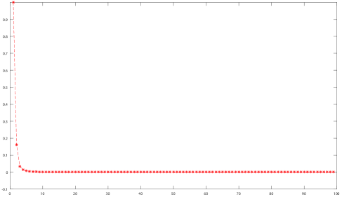
Figure 2: Distribution of ratios $c_{1j}/c_{12}$, $j=2,3,\cdots,M-1$.

As is known, Algorithm 1 is much more expensive for well-conditioned problems than basic iterative techniques, such as conjugate gradient (CG) or (plain) Jacobi iterative method. For the purpose of solving (13) in an optimal way, an adaptive AMG method is proposed below by combining Algorithm 1, the reference formula (33) and the condition number estimation (27) in Corollary 3 as the clear distinction to adaptively pick an appropriate solver.

Algorithm 2

An adaptive AMG method $S_{ad}$ for the linear system (13).

Step 1

If the condition (27) is unsatisfied, then goto Step 2, else set $S_{ad}$ as the CG or Jacobi iterative method;

Step 2

Set $S_{ad}$ as the classical AMG method described in Algorithm 1, with $\theta$ chosen via the reference formula (33).

5 Performance evaluation

Let us illustrate the effectiveness of Algorithms 1 and 2. Numerical experiments are performed in a 64 bit Fedora 18 platform, double precision arithmetic on Intel Xeon (W5590) with 24.0 GB RAM, 3.33 GHz, with an -O2 optimization parameter. In the following tables, dashed entries (-) indicate the solutions either diverge or fail to converge after 1000 iterations, Its is the number of iterations until the stopping criterion $10^{-12}$ is reached, $T_{c}$ represents the CPU time including both Setup and Solve phases with second as its unit, $C_{g}$ and $C_{o}$ respectively denote grid and operator complexities, which are defined as sums of the number of degrees of freedom and nonzero elements on all grid levels divided by those of the finest grid level, and used as measures for memory requirements, aritmetic operations and the execution time in Setup and Solve phases.

Example 2

Comparisons of the classical AMG over CG and Jacobi iterative methods for the case when (27) is satisfied with two different fractional orders.

Table 6: Number of iterations and wall time for the case $\tau=h^{2}$.

$M$	$\alpha=\beta=0.6$						$\alpha=\beta=0.8$
	Jacobi		CG		AMG		Jacobi		CG		AMG
	Its	$T_{c}$	Its	$T_{c}$	Its	$T_{c}$	Its	$T_{c}$	Its	$T_{c}$	Its	$T_{c}$
32	18	1.78E-4	9	1.09E-4	4	5.22E-4	22	2.03E-4	11	1.27E-4	5	2.84E-4
64	18	3.90E-4	11	2.19E-4	4	7.79E-4	23	4.84E-4	13	1.99E-4	5	6.33E-4
128	19	1.31E-3	11	4.60E-4	4	2.52E-3	23	1.54E-3	13	5.26E-4	5	1.89E-3
256	19	4.69E-3	11	1.57E-3	4	9.73E-3	23	5.66E-3	13	1.82E-3	5	7.06E-3
512	19	2.61E-2	11	8.03E-3	4	5.49E-2	23	3.12E-2	13	9.56E-3	5	4.57E-2
1024	19	1.95E-1	11	6.04E-2	4	1.73E-1	23	2.36E-1	12	6.53E-2	5	1.32E-1
2048	19	3.98E-1	11	1.22E-1	4	9.39E-1	23	9.11E-1	12	1.32E-1	5	7.49E-1
4096	19	3.03	11	9.25E-1	4	2.80	23	3.65	12	1.01	5	2.98

As expected, the results in Table 6 show that Jacobi, CG and AMG methods are robust with respect to the mesh size and fractional order, which indicates indirectly the correctness of (23). In addition, CG method runs 3.28 and 3.03 times faster than Jacobi and AMG methods for $M=4096$ and $\alpha=\beta=0.6$, respectively.

Example 3

Comparisons between the classical AMG method and CG method for the case when (27) is unsatisfied.

Table 7: Number of iterations and wall time for the case $\tau=1/32$.

$M$	$\beta=0.6$				$\beta=0.8$				$\beta=0.99$
	CG		AMG		CG		AMG		CG		AMG
	Its	$T_{c}$	Its	$T_{c}$	Its	$T_{c}$	Its	$T_{c}$	Its	$T_{c}$	Its	$T_{c}$
512	97	0.119	8	0.042	180	0.209	8	0.069	256	0.314	3	0.032
1024	147	0.715	8	0.169	314	1.627	8	0.301	512	2.537	3	0.133
2048	223	2.230	8	0.677	546	6.037	8	0.772	$>$1000	-	3	0.532
4096	337	13.378	8	2.735	948	38.481	8	3.143	$>$1000	-	3	2.034

As shown in Table 7, AMG method converges robustly regarding to the mesh size and may be weakly dependent of $\beta$, while the number of iterations of CG method is quite unstable, and sometimes CG method even break down. Furthermore AMG method runs 12.24 times faster than CG method for $M=4096$ and $\beta=0.8$.

Table 8: Number of iterations and wall time for the case $\tau=h$.

$M$	$\alpha=0.2$, $\beta=0.6$				$\alpha=0.6$, $\beta=0.8$
	CG		AMG		CG		AMG
	Its	$T_{c}$	Its	$T_{c}$	Its	$T_{c}$	Its	$T_{c}$
128	40	1.686E-3	8	2.868E-3	57	2.310E-3	7	2.873E-3
256	62	9.090E-3	8	1.571E-2	99	1.622E-2	7	1.081E-2
512	95	1.523E-1	8	6.976E-2	171	2.626E-1	7	4.808E-2
1024	145	5.166E-1	8	2.916E-1	291	1.7895	7	2.063E-1

Table 8 shows the results of $\tau=h$. Despite the advantage in computational cost and robustness over CG method, AMG method is nearly independent of $\alpha$ and $\beta$ in this circumstance. Meanwhile, by an investigation in terms of number of iterations in Tables 7 and 8, CG method converges faster because of the improvement in condition number from $\mathcal{O}(h^{-2\beta})$ to $\mathcal{O}(h^{\alpha-2\beta})$.

Example 4

Comparisons of $S_{ad}$ over the classical AMG and CG methods when the $i$-th time step size $\tau_{i}$ is chosen to be

$$\tau_{i}=\left\{\begin{aligned} &h^{2},~{}\quad i=1,\cdots,K_{1}\\ &1/32,~{}i=K_{1}+1,\cdots,K_{1}+K_{2}\end{aligned}\right..$$

Table 9: Comparisons among $S_{ad}$, CG and AMG.

$K_{2}$	$M=1024$, $K_{1}=K_{2}$						$M=2048$, $K_{1}=K_{2}$
	$S_{\alpha}$		CG		AMG		$S_{\alpha}$		CG		AMG
	Its	$T_{c}$	Its	$T_{c}$	Its	$T_{c}$	Its	$T_{c}$	Its	$T_{c}$	Its	$T_{c}$
25	459	2.09	7994	9.99	303	2.91	458	8.65	13681	71.76	304	12.03
50	909	4.11	15900	19.65	603	5.79	895	17.25	27196	141.81	604	23.79
75	1337	6.54	23748	30.74	903	8.60	1320	25.59	40637	212.48	904	35.76
100	1760	8.54	31573	40.12	1201	11.92	1745	36.07	54038	292.03	1204	50.66
$K_{2}$	$M=1024$, $K_{1}=3K_{2}$						$M=2048$, $K_{1}=3K_{2}$
	$S_{ad}$		CG		AMG		$S_{ad}$		CG		AMG
	Its	$T_{c}$	Its	$T_{c}$	Its	$T_{c}$	Its	$T_{c}$	Its	$T_{c}$	Its	$T_{c}$
25	987	2.86	8522	11.10	553	5.42	970	11.87	14193	79.22	554	21.86
50	1912	5.81	16903	22.57	1088	10.52	1895	22.66	28196	158.78	1091	47.96
75	2837	8.05	25248	31.73	1563	15.23	2820	33.83	42137	230.60	1566	66.73
100	3760	10.82	33573	42.33	2036	20.03	3745	48.37	56038	294.82	2041	83.03

We can observe from Table 9 that $S_{ad}$ and AMG methods are fairly robust as to the mesh size, roughly 10 and 6 on the average. Yet the average number of iterations of CG method varies from 85 to 142. Moreover $S_{ad}$ has a considerable advantage over others in CPU time, runs 1.72 and 6.09 times faster than AMG and CG methods for $M=2048$ and $K_{2}=100$.

Example 5

Analyze effects of the strength-of-connection tolerance $\theta$ on the performance of the classical AMG method.

Table 10: Effect of $\theta$ on the classical AMG when $M=512$.

$\theta$	$\beta=0.8$				$\beta=0.99$
	Its	$T_{c}$	$C_{g}$	$C_{o}$	Its	$T_{c}$	$C_{g}$	$C_{o}$
0.0001	293	1.952	1.037	1.001	103	6.784E-1	1.170	1.021
0.001	83	5.618E-1	1.098	1.008	60	4.189E-1	1.498	1.124
0.00684	31	1.797E-1	1.202	1.029	32	1.374E-1	1.652	1.147
0.00685	31	1.789E-1	1.202	1.029	3	3.255E-1	1.975	1.331
0.01	23	1.020E-1	1.247	1.041	3	3.301E-2	1.975	1.331
0.1	13	6.209E-2	1.489	1.124	3	4.356E-2	1.975	1.331
0.16042	13	6.037E-2	1.489	1.124	3	4.118E-2	1.975	1.331
0.16043	7	4.699E-2	1.975	1.331	3	3.158E-2	1.975	1.331
0.25	7	4.736E-2	1.975	1.331	3	4.353E-2	1.975	1.331
0.5	7	4.710E-2	1.975	1.331	3	4.354E-2	1.975	1.331

Table 11: Effect of $\theta$ on the classical AMG when $M=2048$.

$\theta$	$\beta=0.8$				$\beta=0.99$
	Its	$T_{c}$	$C_{g}$	$C_{o}$	Its	$T_{c}$	$C_{g}$	$C_{o}$
0.0001	335	23.621	1.038	1.001	123	6.310	1.170	1.021
0.001	107	9.024	1.100	1.008	102	5.597	1.497	1.125
0.00684	33	3.096	1.207	1.029	33	2.055	1.662	1.148
0.00685	33	3.129	1.207	1.029	3	7.314E-1	1.993	1.333
0.01	26	2.551	1.249	1.042	3	5.369E-1	1.993	1.333
0.1	15	1.691	1.497	1.125	3	5.448E-1	1.993	1.333
0.1603	15	1.690	1.497	1.125	3	5.372E-1	1.993	1.333
0.1604	8	1.217	1.993	1.333	3	5.294E-1	1.993	1.333
0.2	8	1.219	1.993	1.333	3	5.294E-1	1.993	1.333
0.25	8	1.217	1.993	1.333	3	5.299E-1	1.993	1.333

It is seen from Tables 10 and 11 that there is a unique threshold $\theta_{0}$ independent of $h$ which guarantees the robustness of the classical AMG method, and makes number of iterations of the classical AMG monotonically decreasing when $\theta<\theta_{0}$, or even the classical AMG possibly diverge when $\theta$ is small enough, e.g., $\theta_{0}=0.16043$ and $\theta_{0}=0.00685$ for cases $\beta=0.8$ and $\beta=0.99$. By direct calculations, we have $c_{13}/c_{12}\approx 0.160426$ and $c_{13}/c_{12}\approx 0.006846$. Utilizing the relation (33) and $\epsilon_{0}=10^{-5}$, the corresponding values of $\theta$ are respectively larger than those of $\theta_{0}$. This confirms the reasonability of the reference formula (33).

6 Conclusion

In this paper, we propose the variational formulation for a class of time-space Caputo-Riesz fractional diffusion equations, prove that the resulting matrix is a symmetric Toeplitz matrix, an M-matrix by appending a very weak constraint and its condition number is bounded by $1+\mathcal{O}(\tau^{\alpha}h^{-2\beta})$, introduce the classical AMG method and prove rigorously that its convergence rate is independent of time and space step sizes, provide explicitly a reference formula of the strength-of-connection tolerance to guarantee the robustness and predictable behavior of AMG method in all cases, and develop an adaptive AMG method via our condition number estimation to decrease the computation cost. Numerical results are all in conformity with the theoretical results, and verify the reasonability of the reference formula and the considerable advantage of the proposed adaptive AMG algorithm over other traditional iterative methods, e.g. Jacobi, CG and the classical AMG methods.

References

References

- [1] F. Liu, P. Zhuang, V. Anh, I. Turner, K. Burrage, Stability and convergence of the difference methods for the space-time fractional advection-diffusion equation, Appl. Math. Comput. 191 (1) (2007) 12-20.
- [2] Z. Q. Ding, A. G. Xiao, M. Li, Weighted finite difference methods for a class of space fractional partial differential equations with variable coefficients, J. Comput. Appl. Math. 233 (8) (2010) 1905-1914.
- [3] G. H. Gao, Z. Z. Sun, A compact finite difference scheme for the fractional sub-diffusion equations, J. Comput. Phys. 230 (3) (2011) 586-595.
- [4] S. P. Yang, A. G. Xiao, X. Y. Pan, Dependence analysis of the solutions on the parameters of fractional delay differential equations, Adv. Appl. Math. Mech. 3 (5) (2011) 586-597.
- [5] X. N. Cao, J. L. Fu, H. Huang, Numerical method for the time fractional Fokker-Planck equation, Adv. Appl. Math. Mech. 4 (6) (2012) 848-863.
- [6] H. Wang, T. S. Basu, A fast finite difference method for two-dimensional space-fractional diffusion equations, SIAM J. Sci. Comput. 34 (5) (2012) A2444-A2458.
- [7] M. H. Chen, W. H. Deng, Y. J. Wu, Superlinearly convergent algorithms for the two-dimensional space-time Caputo-Riesz fractional diffusion equation, Appl. Numer. Math. 70 (2013) 22-41.
- [8] D. L. Wang, A. G. Xiao, H. L. Liu, Dissipativity and stability analysis for fractional functional differential equations, Fract. Calc. Appl. Anal. 18 (6) (2015) 1399-1422.
- [9] D. L. Wang, A. G. Xiao, W. Yang, Maximum-norm error analysis of a difference scheme for the space fractional CNLS, Appl. Math. Comput. 257 (2015) 241-251.
- [10] W. Yang, D. L. Wang, L. Yang, A stable numerical method for space fractional Landau-Lifshitz equations, Appl. Math. Lett. 61 (2016) 149-155.
- [11] V. J. Ervin, J. P. Roop, Variational formulation for the stationary fractional advection dispersion equation, Numer. Methods Partial Differ. Equ. 22 (3) (2006) 558-576.
- [12] H. Zhang, F. Liu, V. Anh, Galerkin finite element approximation of symmetric space-fractional partial differential equations, Appl. Math. Comput. 217 (6) (2010) 2534-2545.
- [13] K. Burrage, N. Hale, D. Kay, An efficient implicit FEM scheme for fractional-in-space reaction-diffusion equations, SIAM J. Sci. Comput. 34 (4) (2012) A2145-A2172.
- [14] W. P. Bu, Y. F. Tang, J. Y. Yang, Galerkin finite element method for two-dimensional Riesz space fractional diffusion equations, J. Comput. Phys. 276 (2014) 26-38.
- [15] K. Mustapha, B. Abdallah, K. M. Furati, A discontinuous Petrov-Galerkin method for time-fractional diffusion equations, SIAM J. Numer. Anal. 52 (5) (2014) 2512-2529.
- [16] L. B. Feng, P. Zhuang, F. Liu, I. Turner, Y. T. Gu, Finite element method for space-time fractional diffusion equation, Numer. Algor. 72 (3) (2016) 749-767.
- [17] W. P. Bu, A. G. Xiao, W. Zeng, Finite difference/finite element methods for distributed-order time fractional diffusion equations, J. Sci. Comput. 72 (1) (2017) 422-441.
- [18] F. Liu, P. Zhuang, I. Turner, K. Burrage, V. Anh, A new fractional finite volume method for solving the fractional diffusion equation, Appl. Math. Model. 38 (15-16) (2014) 3871-3878.
- [19] Y. M. Lin, C. J. Xu, Finite difference/spectral approximations for the time-fractional diffusion equation, J. Comput. Phys. 225 (2) (2007) 1533-1552.
- [20] M. Zayernouri, W. R. Cao, Z. Q. Zhang, G. E. Karniadakis, Spectral and discontinuous spectral element methods for fractional delay equations, SIAM J. Sci. Comput. 36 (6) (2014) B904-B929.
- [21] Y. Yang, Y. P. Chen, Y. Q. Huang, Spectral-collocation method for fractional Fredholm integro-differential equations, J. Korean Math. Soc. 51 (1) (2014) 203-224.
- [22] Y. Yang, Y. P. Chen, Y. Q. Huang, Convergence analysis of the Jacobi spectral-collocation method for fractional integro-differential equations. Acta Math. Sci. 34B (3) (2014) 673-690.
- [23] Y. Yang, Jacobi spectral Galerkin methods for fractional integro-differential equations, Calcolo 52 (4) (2015) 519-542.
- [24] Y. Yang, Jacobi spectral Galerkin methods for Volterra integral equations with weakly singular kernel, Bull. Korean Math. Soc. 53 (1) (2016) 247-262.
- [25] S. P. Yang, A. G. Xiao, An efficient numerical method for fractional differential equations with two Caputo derivatives, J. Comput. Math. 34 (2) (2016) 113-134.
- [26] S. L. Lei, H. W. Sun, A circulant preconditioner for fractional diffusion equations, J. Comput. Phys. 242 (2013) 715-725.
- [27] T. Moroney, Q. Q. Yang, A banded preconditioner for the two-sided, nonlinear space-fractional diffusion equation, Comput. Math. Appl. 66 (5) (2013) 659-667.
- [28] J. H. Jia, H. Wang, Fast finite difference methods for space-fractional diffusion equations with fractional derivative boundary conditions, J. Comput. Phys. 293 (2015) 359-369.
- [29] X. M. Gu, T. Z. Huang, X. L. Zhao, H. B. Li, L. Li, Strang-type preconditioners for solving fractional diffusion equations by boundary value methods, J. Comput. Appl. Math. 277 (2015) 73-86.
- [30] M. Donatelli, M. Mazza, S. Serra-Capizzano, Spectral analysis and structure preserving preconditioners for fractional diffusion equations, J. Comput. Phys. 307 (2016) 262-279.
- [31] H. K. Pang, H. W. Sun, Multigrid method for fractional diffusion equations, J. Comput. Phys. 231 (2012) 693-703.
- [32] W. P. Bu, X. T. Liu, Y. F. Tang, J. Y. Yang, Finite element multigrid method for multi-term time fractional advection diffusion equations, Int. J. Model. Simul. Sci. Comput. 6 (2015) 1540001.
- [33] Y. J. Jiang, X. J. Xu, Multigrid methods for space fractional partial differential equations, J. Comput. Phys. 302 (2015) 374-392.
- [34] L. Chen, R. H. Nochetto, E. Otárola, A. J. Salgado, Multilevel methods for nonuniformly elliptic operators and fractional diffusion, Math. Comput. 85 (302) (2016) 2583-2607.
- [35] X. Zhao, X. Z. Hu, W. Cai, G. E. Karniadakis, Adaptive finite element method for fractional differential equations using hierarchical matrices, arXiv: 1603.01358v2.
- [36] J. Xu, Iterative methods by space decomposition and subspace correction, SIAM Rev. 34 (4) (1992) 581-613.
- [37] J. W. Ruge, K. Stüben, Algebraic multigrid, in Multigrid Methods, Front. Appl. Math. 3 (1987) 73-130.
- [38] K. Stüben, An introduction to algebraic multigrid, in Multigrid, U. Trottenberg, C. W. Oosterlee and A. Schüller, eds., Academic Press, Singapore, 2001.