Dynamics beyond dynamic jam; unfolding the Painlevé paradox singularity

Abstract

This paper analyses in detail the dynamics in a neighbourhood of a Génot-Brogliato point, colloquially termed the G-spot, which physically represents so-called dynamic jam in rigid body mechanics with unilateral contact and Coulomb friction. Such singular points arise in planar rigid body problems with slipping point contacts at the intersection between the conditions for onset of lift-off and for the Painlevé paradox. The G-spot can be approached in finite time by an open set of initial conditions in a general class of problems. The key question addressed is what happens next. In principle trajectories could, at least instantaneously, lift off, continue in slip, or undergo a so-called impact without collision. Such impacts are non-local in momentum space and depend on properties evaluated away from the G-spot.

The answer is obtained via an analysis that involves a consistent contact regularisation with a stiffness proportional to $1/\varepsilon^{2}$. Taking a singular limit as $\varepsilon\to 0$, one finds an inner and an outer asymptotic zone in the neighbourhood of the G-spot. Matched asymptotic analysis then enables not just the answer to the question of continuation from the G-spot in the limit $\varepsilon\to 0$ but also reveals the sensitivity of trajectories to $\varepsilon$. The solution involves large-time asymptotics of certain generalised hypergeometric functions, which leads to conditions for the existence of a distinguished smoothest trajectory that remains uniformly bounded in $t$ and $\varepsilon$. Such a solution corresponds to a canard that connects stable slipping motion to unstable slipping motion, through the G-spot. Perturbations to the distinguished trajectory are then studied asymptotically.

Two distinct cases are found according to whether the contact force becomes infinite or remains finite as the G-spot is approached. In the former case it is argued that there can be no such canards and so an impact without collision must occur. In the latter case, the canard trajectory acts as a dividing surface between trajectories that momentarily lift off and those that do not before taking the impact. The orientation of the initial condition set leading to each eventuality is shown to change each time a certain positive parameter $\beta$ passes through an integer.

Finally, the results are illustrated on a particular physical example, namely the a frictional impact oscillator first studied by Leine et al.

1 Introduction

This paper considers the open question first posed in the work of Génot and Brogliato [3] in relation to the classical Painlevé paradox in contact mechanics. They considered the classical problem of a falling rod one end of which is in contact with a rough horizontal surface (see Fig. 1(a)). They show that for sufficiently high coefficient of friction there is an open set of initial conditions that are drawn in finite time into a singularity, which we have termed the G-spot in homage to Génot. Such a point both is characterised by the vanishing of normal free acceleration and the so-called Painlevé parameter which measures the ratio of that acceleration to normal contact force. The physical phenomenon of approaching the singularity is also known as dynamic jam [13] and has been reported in other physical systems. In particular in Sec. 6 below, the results of this paper shall be applied to the frictional impact oscillator system represented in Fig. 1(b), first studied by Leine et al. [8]. Yet, we are unaware of any mathematical analysis of what must happen after such a singularity is reached. Does the rigid body formulation break down completely, so that there is no continuation of trajectories beyond this point? If so, then can we say what might happen physically?

Figure 1: (a) The canonical example of the Painlevé paradox, a rod falling under gravity. (b) The frictional impact oscillator proposed by [8], that we shall return to in Sec. 6.

1.1 The Painlevé paradox and impact without collision

Our work follows the formalism and notation introduced in the recent review paper by two of us [1], to which we refer the reader for the necessary motivation, historical context and general formulation. In particular, there it was argued that approach to a G-spot singularity is a generic mechanism in planar rigid body mechanics subject to unilateral point contact with dry frictional surfaces and is not merely restricted to a few atypical example mechanisms.

Specifically, we consider a multi-degree-of-freedom Lagrangian planar rigid body system with an isolated point of contact with a rigid surface, which is subject to Coulomb friction. Using the notation introduced in [1], we find that projecting the Lagrangian equations of motion onto tangential and normal directions gives scalar equations

$$\dot{u} =a\left(q,\dot{q},t\right)+\lambda_{T}A\left(q,t\right)+\lambda_{N}B\left(q,t\right),$$ (1)

$$\dot{v} =b\left(q,\dot{q},t\right)+\lambda_{T}B\left(q,t\right)+\lambda_{N}C\left(q,t\right).$$ (2)

Here $u$ and $v$ are tangential and normal velocities of the contact point; $q$ is a vector of generalised coordinates and $t$ is time; $a$, $b$, $A$, $B$, $C$, $D$ are scalars subject to the constraints that $A>0$, $C>0$ and $AC-B^{2}>0$ which arise from the assumption of positive definiteness of the mass matrix. The scalars $\lambda_{N}\geq 0$ and $\lambda_{T}$ represent normal and tangential contact forces respectively and are Lagrange multipliers that must be solved for under different assumptions on the mode of motion (free, stick, or positive or negative slip). During contact, we suppose that Coulomb friction applies:

$$|\lambda_{T}|\leq\mu|\lambda_{N}|,\qquad\lambda_{T}=-\mu\>\mbox{sign}(u)\lambda_{N}\quad\mbox{for}\>u\neq 0,$$ (3)

where $\mu$ is the coefficient of friction.

Positive slip occurs during contact with $\lambda_{N}>0$ and $u>0$, so that $\lambda_{T}=-\mu\lambda_{N}$. To sustain contact we must have $\dot{v}=0$, which gives

$$\lambda_{N}=-\frac{b}{p},\qquad\mbox{where}\quad p:=C-\mu B.$$ (4)

Here we dropped the superscript $+$ on the Painlevé parameter $p$, adopted in [1], because this paper shall, without loss of generality, only concern positive slip. If $p$ is negative, we say the Painlevé paradox applies for appropriate initial conditions, in which case (4) shows that in order for $\lambda_{N}$ to be positive we much have free normal acceleration away from the contact, that is $b>0$. This leads to multiplicity of solution, because for $b>0$ lift-off could also occur. However, it can be showed that slipping in regions with $b>0$ is violently unstable [11, 6]. Nevertheless, there is another possibility, and indeed this is the only consistent possibility if $p<0$ and $b<0$, namely that a so-called impact without collision (IWC) occurs, see [10, 1].

Impact in the present context defines a process in which rapid changes in normal and tangential velocity occur over an infinitesimal timescale [15]. The impact process can then be modelled as a composite mapping from an incoming velocity to an outgoing one:

$$(u^{-},v^{-})\mapsto_{\mbox{compression phase}}(u^{(0)},0)\mapsto_{\mbox{restitution phase}}(u^{+},v^{+}),$$ (5)

where $v^{-}\leq 0$ and $v^{+}\geq 0$. In each of the compression and restitution phases, it is assumed that the system behaves as a rigid body system (despite the presence of large forces), and one needs to account for possible transitions from slip to stick. Complete results are summarised in [10], for an energetic coefficient of restitution where the work done by the normal force during restitution is $-r^{2}$ that lost during compression. Similar calculations can be carried out explicitly for a Poisson impact law where the normal impulse in restitution is $-r$ times that in compression (see e.g. [2]). The distinction is not important here. During the impact process, to leading order, the motion can be assumed to occur along straight lines in the $(u,v)$-plane, with corners occurring at transitions between slip and stick during the impact process; see Fig. 2 for two examples.

Figure 2: (a) Representing trajectories during an impact for an initial condition $u>0$ in the case that $p<0$ is small and constant. The solid line indicates a trajectory (labelled (i)) with initial $v<0$, whereas the dashed line indicates a trajectory (ii) undergoing impact without collision, in which the initial condition has $v=0$. (b) Similar Impact events for $p$ small and positive. Here one initial condition lifts off in slip, the other (with smaller initial $u$) lifts off in stick. See [10] for details.

Looking at Fig. 2(a), note that in the case that $p<0$ then we can have an impact even when $v^{-}=0$. This would be an example of an IWC, also known as a tangential shock.

1.2 The G-spot

A question at the heart of the classical Painlevé paradox is what happens next when a configuration with $p=0$ is reached during regular slipping motion. As first shown by Génot and Brogliato [3] for the classical Painlevé paradox (see [1] for a generalisation), in fact the only possible way to approach such a transition is via the codimension-two point in phase space where $p=b=0$, i.e. the G-spot. They analysed nearby trajectories by introducing a singular rescaling of time

$$dt=p\>d\hat{s},$$ (6)

so that the $G$-spot becomes an equilibrium point in suitable variables that evolve on the timescale $\hat{s}$. In so doing, (see Sec. 2 below for details) we obtain a system of the form

$$\frac{d}{d\hat{s}}p = \alpha_{1}p,$$ (7)

$$\frac{d}{d\hat{s}}b = \alpha_{2}p+\alpha_{3}b,$$ (8)

where the $\alpha_{i}$ are constants to leading order, and, depending on the particular system in question can take on any combination of signs.

The dynamics of (7),(8) can be analysed using phase plane analysis. Given an initial condition in slip $(b<0,p>0)$ then there are only three possible outcomes. Either (i) the trajectory remains in slip leaving the vicinity of the G-spot without $b$ or $p$ changing sign; (ii) it lifts off by passing through $b=0$ $p>0$, or (iii) it is attracted to the G-spot $p=b=0$ as $\hat{s}\to\infty$. Note though that $\hat{s}\to\infty$ implies that the G-spot is approached in finite time $t$.

It is straightforward to show that this third possibility can only occur under specific sign combinations of $\alpha_{1}$, $\alpha_{2}$ and $\alpha_{3}$ see [1, Fig. 13]. The three relevant cases are summarised in Fig. 3:

Case I.

If $\alpha_{2}<0$ and $\alpha_{1}<\alpha_{3}<0$ then all initial conditions in the bottom right $(p,b)$-quadrant approach the $G$-spot such that ratio $p/b\to 0$ and the normal force $\lambda_{N}\to\infty$.

Case II.

If $\alpha_{2}>0$ and $\alpha_{1}<\alpha_{3}<0$ then initial conditions with $\alpha_{2}p<(\alpha_{1}-\alpha_{3})b$ similarly approach the $G$-spot with $p/b\to 0$ and $\lambda_{N}\to\infty$.

Case III.

If $\alpha_{2}<0$ and $\alpha_{3}<\alpha_{1}<0$ then the G-spot is approached tangent to the nontrivial eigenvector $\alpha_{2}p=(\alpha_{1}-\alpha_{3})b$ and $\lambda_{N}$ approaches the finite limit $\alpha_{2}/(\alpha_{3}-\alpha_{1})$.

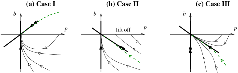
Figure 3: Qualitative illustration of the dynamics of the singular system (7)–(8) in the $(p,b)$ phase plane in each of cases I, II and III with each of the $\alpha$’s assumed to be constant. Here bold lines depict eigenvectors, with double arrows showing the strong stable eigendirection and single arrows the weak stable direction. Thin lines indicate individual trajectories in positive slip which can either be seen to lift-off (by reaching the positive $p$-axis) or to undergo dynamic jam (by reaching the G-spot $b=p=0$. The dashed line (green online) represents the distingished maximally smooth trajectory (see Sec. 5.2 below).

Note that the calculation in [3] reveals that the classical falling rod problem is in Case II. In what follows we shall introduce examples of all three cases.

1.3 Continuation beyond the G-spot and contact regularisation

The rest of this paper concerns what happens for trajectories that pass through G-spot. As we shall see, even that question cannot be answered in complete generality. Our approach though is to to introduce a different scaling than (6) that is singular at $p=0$. In principle, a trajectory passing through the G-spot could continue in (highly unstable) slip with $b>0$, it could lift off, or it could take an IWC (see Fig. 4(a)). However, there is a subtle problem with this latter possibility, as illustrated in Fig. 4(b). Detailed calculations of the impact map (see [10]) reveal that slope of the impacting trajectory in the $(u,v)$-plane is proportional to $p$. But, precisely at the G-spot we know that $p=0$, so one has to consider a different scaling than that used in [10] to calculate the impact map. In principle, as illustrated in Fig. 4(b), the curvature of the impacting trajectory in the $(u,v)$-plane could be such that the impact could terminate at any $u$-value between $u^{-}$ and 0. In other words, we cannot tell a priori whether the impact continues all the way to stick $u=0$, or whether it terminates while the contact is still is slip ($u>0$).

The approach we shall take to addressing these questions is to study the problem via contact regularisation; that is, replacing the rigid constraint with a compliant one whose stiffness scales like some small parameter $\varepsilon^{2}$, see [1] and references therein. In particular, in [11] the idea was introduced of finding resolutions to certain indeterminate cases of the Painlevé paradox via such an approach and taking the limit $\varepsilon\to 0$. If there is a unique solution that can be followed uniformly into this limit, then it was said those dynamics are said to be uniformly resolvable. This enables, for example, questions to be answered of whether slip with $p<0$ could be stably observed in practice (it can’t, it is wildly unstable). This is precisely the approach we shall take here. The key will be to find a consistent asymptotic scaling that enables us to identify a distinguished trajectory that is smooth both in $t$ and $\varepsilon$ in a neighbourhood of the G-spot. Such a maximally smooth trajectory is illustrated as a dashed red line in Figs. 3 and 4. We then consider perturbations to this trajectory to decide whether nearby trajectories take an impact or lift off, and over what timescale.

1.4 Summary of main results

The main result of the paper is to perform a matched asymptotic expansion that enables a description of what happens beyond the G-spot for a general planar rigid body system with an isolated frictional contact point. This is achieved by finding a dinstinguished inner asmyptotic scale for $p$ (or equivalently time) of size $\mathcal{O}\varepsilon^{2/3}$ where $\varepsilon^{-2}$ is the regularised contact stiffness. A matched asymptotic analysis then leads to regular conclusions as $\varepsilon\to 0$. Fig. 4 depicts a qualitative representation of the results for small $\varepsilon>0$. Specifically, we find:

Cases I and II.

As depicted in Fig. 4(e), all trajectories that pass through a small neighbourhood of the G-spot take an IWC. The process of what happens after this impact cannot be analysed by studying the dynamics of a neighbourhood of the G-spot alone, because the impact necessarily involves $O(1)$ changes in $u$ and $v$ (as shown in Fig. 4(b)) and could involve lift off with zero or finite tangential velocity $u$, depending on the precise example system in question.

Case III.

In this case, there is a distinguished trajectory, indicated by a dashed (red) line in Fig. 4(c),(d) that forms a canard solution for small $\varepsilon>0$ which divides two different behaviours. On one side of this distinguished trajectory, solutions lift off, whereas on the other side, they take an IWC. Each time the ratio $\beta=\alpha_{1}/\alpha_{3}$ evaluated at the G-spot passes through a positive integer, then there is side-switching between which sign of perturbation to the canard undergoes lift-off and which undergoes IWC.

More precise statements of these results are given in Secs. 4 and 5 below.

Figure 4: Qualitative representation of the main results. (a) Indicating the scaling of the inner region. Specifically illustrated here is an example of Case III from Fig. 3. In this and subsequent panels, a thick dashed (green online) line is used to represent the distinguished trajectory, thin solid lines (blue online) represent trajectories that lift off after passing through a neighbourhood of the G-spot and thin dashed lines represent trajectories that take an impact without collision. (b) Indicating the process of impact without collision in the (outer) $(u,v)$ co-ordinates in a neighbourhood of the G-spot. Depending on the global dynamics $u$-direction the trajectory can either continue all the way down to stick, or can curve upwards and lift-off while still slipping. (c-e) Representation of dynamics of perturbations to the distinguished trajectory in the inner region: (c) Case III when $[\beta]$ is an odd integer; (d) Case III when $[\beta]$ is even integer; and (e) Case II. (Here $[\cdot]$ represents the integer part of positive number)

1.5 Outline

The rest of this paper is outlined as follows. Section 2 below introduces a general formulation that includes constraint regularisation via an additional degree of freedom, that can be thought of as an additional spring. We also introduce a simple illustrative example system in which many of the calculations can be done explicitly. Sections 3 and 4 then contain numerical and analytical calculations respectively on this example in order to motivate and illustrate the general principles. Section 5 then contains a detailed asymptotic derivation of the main results of the paper for arbitrary planar $m$-dimensional rigid-body system with a single frictional point contact. Section 6 then contains application of the results to the frictional impact oscillator. Finally, Sec. 7 draws conclusions and suggests avenues for other work.

2 Preliminaries

Consider a planar Lagrangian system with a unilateral constraint, which can be expressed in the form $y>0$, where $y$ is a smooth function of the co-ordinate variables $q_{i}$. To simplify notation, in what follows we group together all Lagrangian co-ordinates and velocities variables $q_{i}$, $\dot{q}_{i}$ and (in the case of explicitly non-autonomous systems) $t$ into a single $m$-dimensional state vector $\xi$ and consider systems that are written in the form

$$\dot{\xi}=F(\xi)+G_{T}(\xi)\lambda_{T}+G_{N}(\xi)\lambda_{N},,$$ (9)

where the scalar Lagrange multipliers $\lambda_{N}$ and $\lambda_{T}$ represent the normal and tangential forces at the contact point. We also suppose that tangential and normal contact coordinates $x(\xi)$ and $y(\xi)$ are smooth functions of $\xi$. Now we can express the quantities entering in the normal and tangential equations (1) and (2) as

$$u=\mathsterling_{F}x,\quad v=\mathsterling_{F}y,\quad a=\mathsterling_{F}u,\quad b=\mathsterling_{F}v,\quad A=\mathsterling_{G_{T}}u,\quad B=\mathsterling_{G_{N}}u=\mathsterling_{G_{T}}v,\quad C=\mathsterling_{G_{N}}v$$

where $\mathsterling$ denotes the Lie derivative. In this context, the Lie derivative $\mathsterling_{G}z$ of a scalar function $z(\xi)$ with respect to a vector field $G(\xi)$ is just the total time derivative of $z$ under the assumption that $\xi$ satisfies the dynamical system $\dot{\xi}=G(\xi)$. Additionally, the Lagrangian character of the system requires

$$\mathsterling_{G_{T}}x=\mathsterling_{G_{N}}x=\mathsterling_{G_{T}}y=\mathsterling_{G_{N}}y=0$$ (10)

since $x$ and $y$ do not depend on $\dot{q}$.

If we restrict attention to positive slip, where $\lambda_{T}=-\mu\lambda_{N}$, we obtain

$$\dot{\xi}=F(\xi)+G(\xi)\lambda_{N},$$ (11)

where $G=G_{N}-\mu G_{T}$. We can now further define

$$p=C-\mu B=\mathsterling_{G}v,\quad\alpha_{1}=\mathsterling_{F}p,\quad\alpha_{2}=\mathsterling_{F}b,\quad\alpha_{3}=-\mathsterling_{G}b$$

and again the Lagrangian character requires

$$\mathsterling_{G}p=0.$$ (12)

Under these definitions, in positive slip the scalar quantities $p(\xi)$, $b(\xi)$, $y(\xi)$, $v(\xi)$ satisfy

$$\dot{p} =\alpha_{1}(\xi),$$ (13)

$$\dot{b} =\alpha_{2}(\xi)-\alpha_{3}(\xi)\lambda_{N},$$ (14)

$$\dot{y} =v,$$ (15)

$$\dot{v} =b+p\lambda_{N}.$$ (16)

In what follows will denote by $\xi^{*}$ a point that satisfies the conditions to be at a G-spot in positive slip

$$p(\xi^{*})=b(\xi^{*})=y(\xi^{*})=v(\xi^{*})=0,$$

and use an asterisk to denote functions evaluated at such a point.

2.1 Regularlised contact motion

In the rigid limit, the constraint surface is given by $y(\xi)=0$. Following the approach outlined in the introduction, we shall analyse the system by introducing a regularisation in the form of a smoothing of the contact motion. Here we introduce compliance via an additional degree of freedom with co-ordinate $z$ that represents the vertical deformation of the surface. Then the normal force $\lambda_{N}$ becomes a function of $z$ and the vertical position $y$ of the contact point of the rigid body( Fig. 5)

(a)                                                      (b)

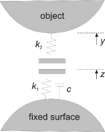
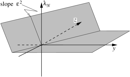
Figure 5: (a) Schematic diagram of the compliant surface model. (b) The compliant normal force versus displacement relationship, which reduces to the usual rigid, unilateral contact law in the limit $\varepsilon\to 0$.

$$c\dot{z}=-k_{1}z-\lambda_{N}$$ (17)

$$\lambda_{N}=\left\{\begin{array}[]{ll}k_{2}(z-y)&\mbox{if }y<z,\\ 0&\mbox{otherwise},\end{array}\right.$$ (18)

where $k_{1,2}$ are $\mathcal{O}(\varepsilon^{-2})$ and $c=\mathcal{O}(\varepsilon^{-1})$ for some small parameter $0<\varepsilon\ll 1$. For convenience in what follows we choose

$$k_{1}=k_{2}=\frac{1}{\varepsilon^{2}},\qquad c=\frac{1}{\varepsilon}.$$ (19)

Note that this form of compliance, via the additional scalar deformation variable $z$, has an advantage over other forms of contact regularisation reviewed in [1] because both lift-off and touch-down are given by the same condition $y=z$. Moreover, as we take the limit $\varepsilon\to 0$, note that $z$ quickly relaxes to be equal to $y/2$ whenever $y<0$ and equal to zero for $y>0$. Moreover, the level of deformation for a given force $\lambda_{N}$ tends to zero as $\varepsilon\to 0$.

It is also worth noting that this impact model is consistent (in the limit of $\varepsilon\rightarrow 0$) with rigid impact models based on coefficients of restitution. For example, our model predicts an ideally elastic impact (energetic coefficient of restitution $=1$ in the sense of [15]) in any of the following limits: $c\rightarrow 0$, $c\rightarrow\infty$, $k_{2}\rightarrow 0$, or $k_{1}\rightarrow\infty$. It predicts ideally inelastic impact (coefficient of restitution $=0$) if $k_{1}\rightarrow 0$ and simultaneously $k_{2}\rightarrow\infty$. Nevertheless fixed values of $k_{1}$, $k_{2}$ and $c$ do not correspond to fixed values of the coefficient of restitution in general.

Using (17)–(19) the compliant version of the system is (9) together with

$$\varepsilon\dot{z} =-z-\varepsilon^{2}\lambda_{N}$$ (20)

$$\lambda_{N} =\left\{\begin{array}[]{ll}\varepsilon^{-2}(z-y)&\mbox{if }y(\xi)<z\\ 0&\mbox{otherwise}\end{array}\right..$$ (23)

and for positive slip (9) becomes (11).

2.2 A simple motivating example

Now, if the quantities $\alpha_{1}$, $\alpha_{2}$ and $\alpha_{3}$ are assumed to be constant in (13)–(16) then we get

$$\dot{p} =\alpha_{1}^{*},$$ (24)

$$\dot{b} =\alpha_{2}^{*}-\alpha_{3}^{*}\lambda_{N},$$ (25)

$$\dot{y} =v,$$ (26)

$$\dot{v} =b+p\lambda_{N},$$ (27)

$$\varepsilon\dot{z} =-z-\varepsilon^{2}\lambda_{N},$$ (28)

where $\lambda_{N}$ is given by (23). Assuming $y<z$ in (23), this set of equations admits a trivial solution

$$\bar{p} =\alpha_{1}^{*}t,$$ (29)

$$\bar{b} =\frac{\alpha_{2}^{*}}{\alpha_{1}^{*}-\alpha_{3}^{*}}\alpha_{1}^{*}t,$$ (30)

$$\bar{z} =\frac{\bar{y}}{2}=-\varepsilon^{2}\frac{\alpha_{2}^{*}}{\alpha_{1}^{*}-\alpha_{3}^{*}},$$ (31)

$$\bar{v} =0$$ (32)

which, as we will see later, is a canard solution that passes through the $G$-spot in the limit $\varepsilon\to 0$.

2.3 A less degenerate example

The question of whether IWC initiated at the G-spot terminates in stick, or in slip (as illustrated in Fig. 4(b)) cannot be determined in the above model because there is no variation of the tangential velocity. Thus the simple system (24)–(28) can never undergo a transition to stick. To allow investigation of such a question, we need to add tangential degrees of freedom to the model via introduction of variables $x$ and

$$\dot{x}=u$$ (33)

representing the tangential position and velocity of the contact point. We also have to include the non-smooth Coulomb friction law. The contact force in stick or slip can be expressed as the sum of a forward slipping and a backward slipping contact forces. Let the magnitude of the normal components of these two forces be given by $\lambda^{+}$ and $\lambda^{-}$, respectively. Specifically we can write

$$\lambda^{+}=c\lambda_{N},\qquad\lambda^{-}=(1-c)\lambda_{N}$$ (34)

where $c=1$ for positive slip, $c=0$ for negative slip, and for stick $c$ takes an intermediate value that shall be determined shortly.

The contact forces corresponding to positive and negative slip have different effects on the dynamics, therefore the terms $\alpha_{3}^{*}\lambda_{N}$ and $p\lambda_{N}$ of (25) and (27) must be replaced by general functions of $\lambda^{+}$ and $\lambda^{-}$. For simplicity in what follows we let the contact-dependent part of $\dot{b}$ be $\alpha_{3}^{*}\lambda^{+}$ and contact-dependent part of $\dot{v}$ be $p\lambda^{+}+p^{-}\lambda^{-}$, where $p^{-}$ is a scalar.

A similar distinction is made in the dynamics of the new variable $u$, which is modelled by the equation

$$\dot{u}=a+k^{+}\lambda^{+}+k^{-}\lambda^{-}$$ (35)

where $a$, $k^{+}$, $k^{-}$ are also scalars. The condition $\dot{u}=0$ for stick now allows us to determine the missing value

$$c=(k^{-}+\lambda_{N}^{-1}a)/(k^{-}-k^{+}).$$ (36)

In addition to the necessary extensions outlined above, we also introduce a parametric state dependence of $\alpha_{1}$ in the form of $\alpha_{1}(\xi)=\alpha_{1}^{*}+\chi b$, for some scalar $\chi$ which allows two-way coupling between normal and tangential dynamics. The resulting extended example system can now be written in the form (23), (33), (35) and

$$\dot{p} =\alpha_{1}^{*}+\chi b,$$ (37)

$$\dot{b} =\alpha_{2}^{*}-c\alpha_{3}^{*}\lambda_{N}$$ (38)

$$\dot{y} =v,$$ (39)

$$\dot{v} =b+pc\lambda_{N}+p^{-}(1-c)\lambda_{N},$$ (40)

$$\varepsilon\dot{z} =-z-\varepsilon^{2}\lambda_{N},$$ (41)

in which $\chi$, $\alpha^{*}_{1-3}$, $k^{\pm}$ and $a$ are fixed constants and $c$ is given by (36) for stick and is equal to 0 or 1 for negative and postive slip respectively.

If $p\approx 0$ then the negative Painlevé parameter must be positive [1], hence we choose $p^{-}=1$. Finally, positive (respectively, negative) slipping contact forces typically accelerate the contact point in the negative (positive) tangential direction, which motivates the choice

$$p^{-}=1,\quad k^{+}=-1,\quad k^{-}=2\quad\mbox{and}\quad a=0.$$ (42)

where the choice $a=0$ is simply made for convenience.

Note that this extended example system (23), (33)-(35) and (37)–(42) was not explicitly derived from a Lagrangian system, nevertheless it can be written in the form (9) by taking

$$F(\xi)=\begin{pmatrix}\xi_{2}\\ 0\\ \xi_{4}\\ \xi_{6}\\ \alpha_{1}^{*}+\chi\xi_{6}\\ \alpha_{2}^{*}\end{pmatrix},\quad G_{T}(\xi)=\begin{pmatrix}0\\ \frac{3}{2(1-\xi_{5})}\\ 0\\ \frac{1}{2}\\ 0\\ \frac{\alpha_{3}^{*}}{2(1-\xi_{5})}\end{pmatrix},\quad G_{N}(\xi)=\begin{pmatrix}0\\ \frac{1}{2}\\ 0\\ \frac{1+\xi_{5}}{2}\\ 0\\ -\frac{\alpha_{3}^{*}}{2}\end{pmatrix},\quad\mu=1-\xi_{5},\quad x=\xi_{1},\quad y=\xi_{3}.$$

and it satisfies the relations (10), (12), which reflect the Lagrangian character of general systems. It then follows that

$$u=\xi_{2},\quad v=\xi_{4},\quad p=\xi_{5},\quad b=\xi_{6},\quad\alpha_{1}=\alpha_{1}^{*}+\chi\xi_{6},\quad\alpha_{2}=\alpha_{2}^{*},\quad\alpha_{3}=\alpha_{3}^{*}.$$

Note that the parameter $\chi$ can be effectively thought of as a homotopy parameter that allows us to pass from a simple case ($\chi=0$) in which there is a trivial solution (similar to (29)–(32)) that passes through the $G$-spot to a more complicated case ($\chi=1$) in which there is no such trivial solution.

3 Numerical results for motivating example

We consider first the simplified version of the motivating example (24)–(28). We want to understand what happens to initial conditions that are small perturbations from the trivial solution (29)–(32).

3.1 A dichotomy between lift-off and impact

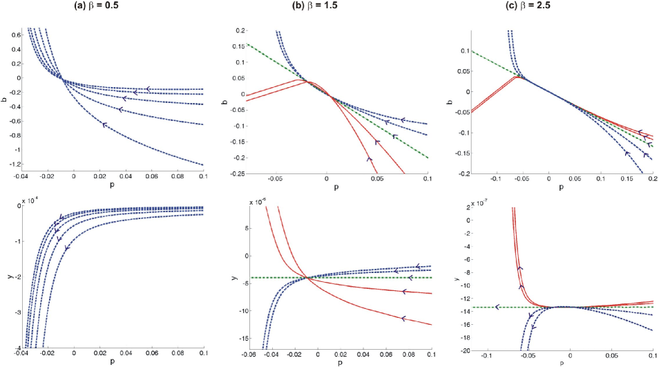
Figure 6: Numerical simulation of (24)–(27) for $\varepsilon=10^{-3}$ with $\alpha_{1}^{*}=\alpha_{2}^{*}=-1$ and $\alpha_{3}^{*}=-\beta$, where; (a) $\beta=0.5$, (b) $\beta=1.5$, or (c) $\beta=2.5$. Initial conditions in each case are $p(0)=0.5$; $b(0)=-|\nu\cdot p(0)\alpha_{2}^{*}/(\alpha_{3}^{*}-\alpha_{1}^{*})|$ where $\nu=0.25$, $0.5$, 1, 2, 4 $y(0)=2\varepsilon^{2}b(0)/p(0)$, $z(0)=\varepsilon^{2}b(0)/p(0)$, $v(0)=0$. In each plot, a dot-dashed (green online) line depicts the trivial solution, solid (red online) curves represent trajectories that lift off, whereas dashed (blue online) curves represent trajectories that take an IWC.

First of all, note that the internal dynamics of the compliant contact model creates damped oscillations. Clearly, this is an artefact of our contact model and not important to our discussion. Note though an important feature of these oscillations is that their frequency diverges to $\infty$ in the limit of $\varepsilon\rightarrow 0$. This lack of smoothness allows us to separate this component of the dynamics in any subsequent analysis. In our preliminary simulations we minimise transient oscillations by choosing initial conditions satisfying $z=y/2$, $v=0$ and $y=2b\varepsilon^{2}/p$ and by choosing an initial value $p=0.5$, which is sufficiently distant from the G-spot to allow for the $z$ dynamics to relax.

The results of three simulations for different values of the scalar parameter

$$\beta=\frac{\alpha_{3}^{*}}{\alpha_{1}^{*}}$$ (43)

are presented in Fig. 6. Panel (a) of the figure corresponds to Case I where $\alpha_{1}^{*}<\alpha_{3}^{*}<0$. Here we see that for all initial conditions that become attracted to the G-spot, $y$ diverges to $-\infty$, which indicates the onset of an IWC. The trivial solution in this case is unphysical ($bp>0$, implying $\lambda_{N}<0$) and is not shown. We found the results in Case II to be similar, that is, all initial conditions that pass the G-spot take an impact.

Panels (b) and (c) of Fig. 6 illustrate two different examples of Case III where $\beta$ is 1.5 and 2.5, respectively. Here we see that there is a dichotomy, in that there are some trajectories that immediately lift off (which can be seen because $y$ increases rapidly), whereas other trajectories take an IWC. The trivial solution appears to form a separatrix between these two behaviours. Interestingly, the set of initial conditions that impact or lift off are swapped, between the two examples shown. That is, initial conditions with lower initial values of $b(0)$ are the ones that take an impact in panel (b) whereas it is those with the higher $b(0)$ that take an impact in panel (c).

3.2 Smoothness in the limit of $\varepsilon\rightarrow 0$

The trajectories presented above not only differ in their asymptotic behaviour for large times, but also in their degree of smoothness as a function of time in the limit $\varepsilon\rightarrow 0$. To illustrate this property, we have repeated the same simulations with $\varepsilon=10^{-5}$. The results are illustrated as plots of $y$ as a function of $p$ in Fig. 7 for all three values of $\beta$. Note that $p$ scales linearly with time. The trivial separatrix solutions appear for $\beta=1.5$ and 2.5 as a straight line, which is by definition, infinitely smooth. At the same time, all other trajectories show some kind of divergence as $p\to 0$. For $\beta=0.5$, $y$ appears to to diverge to infinity in the limit of small $p$. In contrast, for $\beta=1.5$, the first derivative of $y$ appears to diverge. For $\beta=2.5$, a more detailed analysis (not shown) shows divergence of the second derivative of $y$. As we shall see shortly, systematic variation of $\varepsilon$ also confirms these observations.

Now, for the simple model system, we have a trivial solution that forms the separatrix. For more general systems (as for example (37)–(42) with $\chi=1$) we shall demonstrate in Sec. 5 below that there nevertheless exists a separatrix trajectory in Case III, which preserves a higher degree of smoothness in the limit $\varepsilon\rightarrow 0$ than any other trajectory. Specifically, the method of construction will be used to develop an expansion for the trajectory that is at least $C^{\infty}$ in $t$ and $\varepsilon$. This property enables us to disregard all other trajectories (either with or without oscillatory components) that are less smooth in the limit $\varepsilon\to 0$.

Figure 7: Numerical simulation of (24)–(27) for $\varepsilon=10^{-5}$ with: dot-dashed line (green online) $\beta=0.5$; dashed line (red online) $\beta=1.5$; and solid line (blue online) $\beta=2.5$. Other values are the same as in previous simulations.

3.3 Asymptotic behaviour for $\varepsilon\rightarrow 0$

Our analysis of the dynamics near the G-spot will make use of a carefully chosen inner scaling of the variables. To motivate the particular scaling chosen in Sec. 5, we now present the numerically observed dependence on $\varepsilon$ of the dynamics of the model system. We will use letters with a hat ( $\hat{}$ ) for the deviation of variables $p$, $b$, $y$, $v$, $z$ from their values along the trivial solution, for example.

$$b(t,\varepsilon)=\bar{b}(t,\varepsilon)+\hat{b}(t,\varepsilon).$$

To learn how $\hat{b}$, $\hat{y}$ and $\hat{v}$ scale as $\varepsilon\rightarrow 0$, we have recorded their values at the time of passing the G-spot ($p=0$) in a series of simulations where $\varepsilon$ was varied systematically. Three values of $\beta$ were considered and the initial conditions used were the same as in the caption of Fig. 6 with $\nu=2$. The results for $\hat{b}$ are depicted in Fig. 8. We found a nearly perfect power-law relationship $\hat{b}\approx\varepsilon^{\gamma}$ for constant times determined by $p=0$, at least for sufficiently small $\varepsilon$, where the exponent $\gamma$ was determined by linear regression, see Table 1(a). Similar results were obtained for $\hat{v}$ and $\hat{y}$.

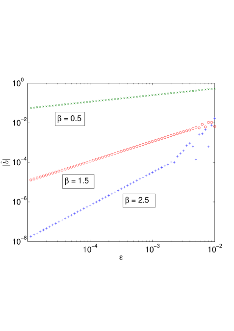
Figure 8: Logarithmic plot of $\hat{b}$ at the time when $p=0$ as $\varepsilon$ varies, for a perturbed initial condition close to the $G$-spot. See text for details.

In a similar manner, we have also measured the time difference between passing the G-spot ($p=0$) and crossing $\hat{b}=0$, see the last row of the table. Clearly the exponent of the time-difference is close to 2/3 whereas other exponents appear to depend on $\beta$ linearly. The general asymptotic theory in Secs. 4 and 5 below predict that these exponents should, in the limit $\varepsilon\to 0$, take the values $2\beta/3$ ($\hat{b}$), $(2\beta+2)/3$ ($\hat{v}$) and $(2\beta+4)/3$ ($\hat{y}$). Table 1(b) gives the theoretical values according to these formulae. We see that there is excellent agreement with the numerical findings.

	(a) Measured			(b) Theoretical
	$\beta=0.5$	$\beta=1.5$	$\beta=2.5$		$\beta=0.5$	$\beta=1.5$	$\beta=2.5$
exponent for $\hat{b}$	0.3326	0.9982	1.6635	$2\beta/3$	0.3333	1.0	1.6667
exponent for $\hat{v}$	0.9983	1.6652	2.3396	$(2\beta+2)/3$	1.0	1.6667	2.3333
exponent for $\hat{y}$	1.6538	2.3384	2.9808	$(2\beta+4)/3$	1.6667	2.3333	3.000
exponent for $t$	0.6650	0.6656	0.6659	$2/3$	0.6667	0.6667	0.6667

Table 1: (a) Numerically measured scaling exponents $\gamma$ such that the named quantity in the first column scales like $\varepsilon^{\gamma}$ as $\varepsilon\rightarrow 0$. (b) Theoretical values of these exponents according to the asymptotic theory of Secs. 4 and 5.

3.4 Possible dynamics beyond the G-spot

The above dynamics simply illustrate the scaling of trajectories and whether they lift off or take an IWC. What happens after these two possible events is also interesting in its own right. Firstly, after lift-off we have $\lambda_{N}=0$, and thus $\dot{b}=\alpha_{2}^{*}$. In Case II, $\dot{b}>0$, which means that $b$, $y$ and $v$ will increase, and lift-off will persist for some time. Nevertheless in Cases I and III, $\dot{b}<0$, which eventually cause $v$ and $y$ to decrease as well. Hence, lift-off will — at least in the limit of $\varepsilon\rightarrow 0$ — always terminate shorty after passing the G-spot, and an impact with very low pre-impact normal velocity (i.e. a quasi-IWC) will occur.

In order to examine what happens once an IWC is initiated, we have to consider the extended version of the example system (23), (33)-(35) and (37)–(41), which includes tangential dynamics and possible transitions from slip to stick.

Two simulations are presented in Fig. 9. In each one, we use the same parameter values and some of the initial conditions used in Fig. 6(a), but compute for a longer timespan. The initial value of $u$ is $u(0)=70$ whereas the initial value of $x(0)$ is arbitrary, since $x$ is a cyclic coordinate. Furthermore we use $\chi=0$ in the first simulation and $\chi=1$ in the second. In the first case (continuous curve, red online), we observe that the near-tangential impact continues all the way until the contact sticks ($\dot{u}=0$). However in the second (dashed curve, blue online), the large contact force initiates a rapid increase of $b$ (due to $\alpha_{3}^{*}<0$). For large enough $u(0)$, the variables $p$, $v$ and $y$ all begin to increase before the contact sticks. In this case the impact will terminate and a lift-off occur before we reach all the way to $u=0$.

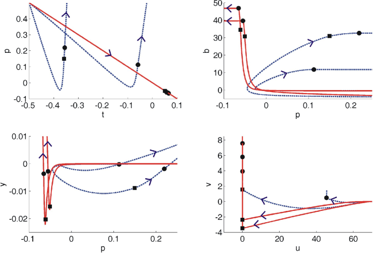
Figure 9: Two-dimensional projections of simulation results of the extended model system with $u(0)=70$ and $\chi=0$ (solid curve, red online) or $\chi=1$ (dashed curve, blue online). Other parameter values are as in Fig. 6(a) except that results for two different $\nu$-values are shown, namely $\nu=0.25$ and $4$. Squares and circles denote slip-stick transitions and liftoff, respectively. Notice that liftoff occurs without slip-stick transition in one out of four cases.

4 Asymptotic analysis of the motivating example

Before presenting general analysis, it is useful to explore the major ideas using the simplified version of the model system (24)–(28) for which the details are eased because of the existence of a trivial smoothest solution (29)–(32). We assume throughout that the system is in contact, so that

$$\varepsilon^{2}\lambda_{N}=z-y,$$

and we suppose that $\alpha_{1}^{*}<0$, $\alpha_{3}^{*}<0$.

If we fix the origin of time so $p(0)=0$, then $p(t)=\alpha_{1}^{*}t$. Inserting this into the other equations, we can eliminate $y$, $v$, and $\lambda_{N}$ by differentiating the $\dot{b}$ equation with respect to time three times and eliminating $z$ and its derivatives via

$$\alpha_{3}^{*}(z-y)=\varepsilon^{2}\left(\alpha_{2}-\frac{db}{dt}\right),\qquad\alpha_{3}^{*}(\dot{z}-\dot{y})=-\varepsilon^{2}\frac{d^{2}b}{dt^{2}},\qquad\alpha_{3}^{*}(\ddot{z}-\ddot{y})=-\varepsilon^{2}\frac{d^{3}b}{dt^{3}}.$$

We obtain

$$\alpha_{3}^{*}b+\alpha_{1}^{*}t\left(\alpha_{2}^{*}-\frac{db}{dt}\right)+\varepsilon\left[\alpha_{3}^{*}\frac{db}{dt}+\alpha_{1}^{*}\left(\alpha_{2}^{*}-\frac{db}{dt}\right)-\alpha_{1}^{*}t\frac{d^{2}b}{dt^{2}}\right]-2\varepsilon^{2}\frac{d^{3}b}{dt^{3}}-\varepsilon^{3}\frac{d^{4}b}{dt^{4}}=0,$$

which is a more convenient 3rd-order single equation for $b(t)$. Note that the other variables can be recovered via

$$\alpha_{3}^{*}y =\varepsilon^{2}\left[\alpha_{3}^{*}b+\alpha_{1}^{*}t\left(\alpha_{2}^{*}-\frac{db}{dt}\right)-2\left(\alpha_{2}^{*}-\frac{db}{dt}\right)\right]-\varepsilon^{3}\frac{d^{2}b}{dt^{2}}-\varepsilon^{4}\frac{d^{3}b}{dt^{3}},$$ (44)

$$\alpha_{3}^{*}v =-\varepsilon\left[\alpha_{3}^{*}b+\alpha_{1}^{*}t\left(\alpha_{2}^{*}-\frac{db}{dt}\right)\right]+2\varepsilon^{2}\frac{d^{2}b}{dt^{2}}+\varepsilon^{3}\frac{d^{3}b}{dt^{3}},$$ (45)

$$\alpha_{3}^{*}z =\varepsilon^{2}\left[\alpha_{3}^{*}b+\alpha_{1}^{*}t\left(\alpha_{2}^{*}-\frac{db}{dt}\right)-\left(\alpha_{2}^{*}-\frac{db}{dt}\right)\right]-\varepsilon^{3}\frac{d^{2}b}{dt^{2}}-\varepsilon^{4}\frac{d^{3}b}{dt^{3}},$$ (46)

$$\alpha_{3}^{*}\lambda_{N} =\alpha_{2}^{*}-\frac{db}{dt}.$$ (47)

We now want to find a time rescaling to de-singularise the $G$-spot. One possibility would be to rescale time using the value of $p$, (6), leading to (7)–(8) as in [3]. Unfortunately, such a rescaling is too brutal to obtain information on what happens beyond the G-spot, not least because the system can only be defined for $p>0$. Instead, we shall seek a scaling in terms of the parameter $\varepsilon$ of the contact regularised system. In so doing we will get an outer dynamical system, which will take the form of a fast-slow system [7]. Then we introduce a new inner timescale which is $\mathcal{O}(\varepsilon^{2/3})$. This gives the ability to find a distingished limit in which the singularity associated with the $G$-spot is balanced by the contact dynamics.

4.1 A distinguished trajectory

We shall start by considering the explicit trivial solution (29)–(32). Note that this solution is smooth in both the variables $t$ and $\varepsilon$. If the parameter $\beta$ (see 43) is not an integer, we will now show that it is the only solution that is smooth in $t$ and $\varepsilon$, and thus we designate it as the distinguished trajectory.

Such a smooth trajectory must have an expansion in $\varepsilon$

$$\bar{b}(t,\varepsilon)=\sum_{n}b_{n}(t)\varepsilon^{n}$$

such that each $b_{n}(t)$ is a smooth function. Inserting this into (4), we find to order $\varepsilon^{0}$ that

$$\alpha_{3}^{*}b_{0}+\alpha_{1}^{*}t\left(\alpha_{2}^{*}-\frac{db_{0}}{dt}\right)=0,$$

which has general solution

$$b_{0}(t)=\frac{\alpha_{2}^{*}}{1-\beta}t+\begin{cases}C_{1}(-t)^{\beta}&\text{if $t\leq 0$}\\ C_{2}(t)^{\beta}&\text{if $t\geq 0$}\end{cases}.$$

Since $\beta$ is not an integer, $b_{0}$ is not smooth unless $C_{1}=C_{2}=0$. Inserting this solution into the order $\varepsilon^{1}$ equation we get

$$\alpha_{3}^{*}b_{1}-\alpha_{1}^{*}t\frac{db_{1}}{dt}=0,$$

and again smoothness forces $b_{1}(t)=0$. Proceeding similarly, at $\mathcal{O}(\varepsilon^{n})$, we get

$$\alpha_{3}^{*}b_{n}-\alpha_{1}^{*}t\frac{db_{n}}{dt}=0$$

and thus we need to choose $b_{n}(t)=0$ for all $n>0$.

Hence the requirement of smoothness leads uniquely to

$$\bar{b}(t,\varepsilon)=\frac{\alpha_{2}^{*}}{1-\beta}t,$$

from which we can recover the rest of the trivial solution (29)–(32), for the variables $y$, $v$ and $z$ using (44)–(46).

4.2 Deviations from the distinguished trajectory: outer scaling

We now wish to consider trajectories whose initial conditions near the G-spot are small perturbations from the distinguished trajectory. Recall that $\hat{b}$ denotes deviations from $\bar{b}$. Then, $\hat{b}$ satisfies

$$\alpha_{3}^{*}\hat{b}-\alpha_{1}^{*}t\frac{d\hat{b}}{dt}+\varepsilon\left[\left(\alpha_{3}^{*}-\alpha_{1}^{*}\right)\frac{d\hat{b}}{dt}-\alpha_{1}^{*}t\frac{d^{2}\hat{b}}{dt^{2}}\right]-2\varepsilon^{2}\frac{d^{3}\hat{b}}{dt^{3}}-\varepsilon^{3}\frac{d^{4}\hat{b}}{dt^{4}}=0,$$ (48)

while the deviations of the other variables from the distinguished trajectory can be recovered using

$$\alpha_{3}^{*}\hat{y} =\varepsilon^{2}\left[\alpha_{3}^{*}\hat{b}-\alpha_{1}^{*}t\frac{d\hat{b}}{dt}+2\frac{d\hat{b}}{dt}\right]-\varepsilon^{3}\frac{d^{2}\hat{b}}{dt^{2}}-\varepsilon^{4}\frac{d^{3}\hat{b}}{dt^{3}}$$ (49)

$$\alpha_{3}^{*}\hat{v} =-\varepsilon\left[\alpha_{3}^{*}\hat{b}-\alpha_{1}^{*}t\frac{d\hat{b}}{dt}\right]+2\varepsilon^{2}\frac{d^{2}\hat{b}}{dt^{2}}+\varepsilon^{3}\frac{d^{3}\hat{b}}{dt^{3}}$$ (50)

$$\alpha_{3}^{*}\hat{z} =\varepsilon^{2}\left[\alpha_{3}^{*}\hat{b}-\alpha_{1}^{*}t\frac{d\hat{b}}{dt}+\frac{d\hat{b}}{dt}\right]-\varepsilon^{3}\frac{d^{2}\hat{b}}{dt^{2}}-\varepsilon^{4}\frac{d^{3}\hat{b}}{dt^{3}}$$ (51)

$$\alpha_{3}^{*}\hat{\lambda}_{N} =-\frac{d\hat{b}}{dt}.$$ (52)

Assuming $t$ is not close to zero, we can identify two timescales in (48); a slow timescale of order $\mathcal{O}(1)$ and a fast timescale of order $\mathcal{O}(\varepsilon)$.

The fast system.

Introducing a fast timescale $t_{f}$ via $dt=\varepsilon dt_{f}$, and reintroducing $p=\alpha_{1}^{*}t$, we find that equation (48) becomes

$$-\left[p\left(\frac{d\hat{b}}{dt_{f}}+\frac{d^{2}\hat{b}}{dt_{f}^{2}}\right)+2\frac{d^{3}\hat{b}}{dt_{f}^{3}}+\frac{d^{4}\hat{b}}{dt_{f}^{4}}\right]+\varepsilon\left[\alpha_{3}^{*}\hat{b}+\left(\alpha_{3}^{*}-\alpha_{1}^{*}\right)\frac{d\hat{b}}{dt_{f}}\right]=0.$$

Setting $\varepsilon=0$, thus treating $p$ as a constant, and looking for exponential solutions to the resulting linear constant coefficient equation, we get the characteristic polynomial

$$-\lambda\left[\lambda^{3}+2\lambda^{2}+p\lambda+p\right]=0$$

where the first factor gives a zero root corresponding to the slow time scale, whereas the non-trivial second factor corresponds to the dynamics of the fast system. For this second factor, if $p>0$, the Routh-Hurwith criterion implies that all roots have negative real parts, hence the fast subsystem is stable. Hence, for $p>0$ trajectories are attracted to a codimension-three manifold, representing the slow dynamics.

In contrast, if $p<0$, then the discriminant of the second factor $\Delta=-p(4(p)^{2}-13p+32)$ is always positive, which means that the fast system has three real eigenvalues. Note further that the sum of the eigenvalues is $-2$ whereas their product is $-p$, which implies that precisely one eigenvalue out of the the three is positive for $p<0$. Hence the slow dynamics for $p<0$ is normally hyperbolic with a two-dimensional stable manifold and one-dimensional unstable manifold.

The slow system

is obtained from (48) by letting $\varepsilon\rightarrow 0$ so that we obtain

$$\alpha_{3}^{*}\hat{b}-\alpha_{1}^{*}t\frac{d\hat{b}}{dt}=0,$$

with solution

$$\hat{b}(t)=\begin{cases}C_{1}(-t)^{\beta}&\text{if $t\leq 0$}\\ C_{2}(t)^{\beta}&\text{if $t\geq 0$}\\ \end{cases}$$ (53)

and

$$\frac{\hat{y}}{\varepsilon^{2}}=2\frac{\hat{b}}{\alpha_{1}^{*}t},\quad\frac{\hat{v}}{\varepsilon}=0,\quad\frac{\hat{z}}{\varepsilon^{2}}=\frac{\hat{b}}{\alpha_{1}^{*}t},\quad\hat{\lambda}_{N}=-\frac{\hat{b}}{\alpha_{1}^{*}t},\quad\beta=\frac{\alpha_{3}^{*}}{\alpha_{1}^{*}}.$$

4.3 Inner scaling

When $t$ is close to zero, we can introduce a rescaled time variable via

$$t=\delta^{2}s,\qquad\mbox{where}\quad\delta=\varepsilon^{1/3},$$

in accordance with the observations in Table 1(a). Under such a rescaling, (48) becomes

$$\alpha_{3}^{*}\hat{b}-\alpha_{1}^{*}s\frac{d\hat{b}}{ds}-2\frac{d^{3}\hat{b}}{ds^{3}}+\delta\left[\left(\alpha_{3}^{*}-\alpha_{1}^{*}\right)\frac{d\hat{b}}{ds}-\alpha_{1}^{*}s\frac{d^{2}\hat{b}}{ds^{2}}-\frac{d^{4}\hat{b}}{ds^{4}}\right]=0.$$ (54)

Again we can identify two timescales: a slow timescale of order $\mathcal{O}(\varepsilon^{2/3})$ ($\mathcal{O}(1)$ in $s$), and a fast timescale of order $\mathcal{O}(\varepsilon)$ ($\mathcal{O}(\varepsilon^{1/3})$ in $s$).

The fast time scale

is defined by defining a new time variable $s_{f}$ so that $ds=\delta ds_{f}$. From this, (54) becomes

$$-2\frac{d^{3}\hat{b}}{ds_{f}^{3}}-\frac{d^{4}\hat{b}}{ds_{f}^{4}}+\delta^{2}\alpha_{1}^{*}s\left(\frac{d\hat{b}}{ds_{f}}+\frac{d^{2}\hat{b}}{ds_{f}^{2}}\right)+\delta^{3}\left[\alpha_{3}^{*}\hat{b}+\left(\alpha_{3}^{*}-\alpha_{1}^{*}\right)\frac{d\hat{b}}{ds_{f}}\right]=0.$$

Letting $\varepsilon\rightarrow 0$ we have a characteristic equation $-\lambda^{3}\left[\lambda+2\right]=0$. There are three zero roots corresponding to the slow time scale, and one real root $\lambda=-2$. We conclude that the fast system is stable.

The slow timescale

is obtained by letting $\delta\rightarrow 0$ in (54) from which we obtain

$$\alpha_{3}^{*}\hat{b}-\alpha_{1}^{*}s\frac{d\hat{b}}{ds}-2\frac{d^{3}\hat{b}}{ds^{3}}=0.$$ (55)

This equation has solutions that can be expressed in terms of generalised hypergeometric functions. Specifically, upon rescaling

$$\tau=\kappa s,\qquad\mbox{with}\quad\kappa=(-\alpha_{1}^{*}/2)^{1/3}>0$$

and setting $b(s)=\theta(\tau)$ we get

$$\frac{d^{3}}{d\tau^{3}}\theta-\tau\frac{d}{d\tau}\theta+\beta\theta=0,$$ (56)

for

$$\beta=\alpha_{3}^{*}/\alpha_{1}^{*}.$$

The equation (56) has a solution that can be expressed in terms of generalised hypergeometric functions, whose asymptotic properties are summarised in Appendix A. From that solution, we can recover all other variables from $\hat{b}$ via

$$\delta^{2}\alpha_{3}^{*}\frac{\hat{y}}{\varepsilon^{2}}=2\frac{d\hat{b}}{ds},\quad\delta^{2}\alpha_{3}^{*}\frac{\hat{v}}{\varepsilon}=2\frac{d^{2}\hat{b}}{ds^{2}},\quad\delta^{2}\alpha_{3}^{*}\frac{\hat{z}}{\varepsilon^{2}}=\frac{d\hat{b}}{ds},\quad\delta^{2}\alpha_{3}^{*}\hat{\lambda}_{N}=-\frac{d\hat{b}}{ds}.$$ (57)

4.4 Matching the inner and outer solutions

We know that the outer solution behaves like

$$\hat{b}(t)\sim C_{1}(-t)^{\beta}\qquad\mbox{as}\quad t\rightarrow 0^{-}.$$ (58)

and this must match the behaviour of the inner solution $\hat{b}(s)$ as $s\rightarrow-\infty$.

The asymptotics of the solution inner region $s\to\pm\infty$ can be established from the asymptotic behavour of $\theta(\tau)$, given by (56) which is studied in Appendix A. The general solution is a linear combination of a function $h$ with power-law type behaviour and two rapidly oscillating functions $e_{r}$ and $e_{i}$. To get the desired behaviour, the coefficients of $e_{r}$ and $e_{i}$ must vanish, and there is a unique solution $\Theta(\tau,\beta)$ that behaves like $(-\tau)^{\beta}$ as $\tau\rightarrow-\infty$.

Matching with the small $t$ limit (58) with the large negative $\tau$ limit, we find that the leading-order inner solution matches if we take it to be

$$\hat{b}(s)=C_{1}\kappa^{-\beta}\varepsilon^{2\beta/3}\Theta(\kappa s,\beta)\sim C_{1}\kappa^{-\beta}\varepsilon^{2\beta/3}(-\kappa s)^{\beta}=C_{1}(-\varepsilon^{2/3}s)=C_{1}(-t)^{\beta},$$ (59)

where again $\kappa=(-\alpha_{1}^{*}/2)^{\frac{1}{3}}$.

Combining (59) with (57), we find the scaling for all the perturbation variables of the inner solution

$$\hat{b}(s) = \mathcal{O}(\varepsilon^{2\beta/3}),$$

$$\hat{y}(s) = \mathcal{O}(\varepsilon^{(2\beta+4)/3}),$$

$$\hat{v}(s) = \mathcal{O}(\varepsilon^{(2\beta+2)/3}),$$

$$\hat{z}(s) = \mathcal{O}(\varepsilon^{(2\beta+4)/3}),$$

$$\hat{\lambda}_{N}(s) = \mathcal{O}(\varepsilon^{(2\beta-2)/3}),$$

when $s=\mathcal{O}(1)$. Recalling that $t=\varepsilon^{2/3}s$, we obtain the theoretical predictions given in Table 1.

4.5 Interpretation for the dynamics

To determine whether lift-off ($\lambda_{N}=0$) or impact-like behaviour ($\lambda_{N}$ large) occurs for the inner solution we study

$$\lambda_{N}=\bar{\lambda}_{N}+\hat{\lambda}_{N}=\frac{\alpha_{2}^{*}}{\alpha_{1}^{*}-\alpha_{3}^{*}}-\frac{C_{1}}{\alpha_{3}^{*}}\kappa^{1-\beta}\varepsilon^{(2\beta-2)/3}\frac{d\Theta}{d\tau}(\tau,\beta).$$

In $\hat{\lambda}_{N}$, we must consider that $\varepsilon^{(2\beta-2)/3}$ is very large or very small depending on whether $\beta<1$ or $\beta>1$. If $\beta<1$, a sign change from positive to negative for $C_{1}d\Theta/d\tau$ means lift-off, whereas a positive sign throughout means impact. If $\beta>1$, the size of $d\Theta/d\tau$ must be very large to have any effect. From Theorems 5 and 6 in Appendix A, we know that

$$\frac{d\Theta}{d\tau}(\tau,\beta)\begin{cases}\text{is negative}&\text{ for $\tau$ large and negative,}\\ \text{has sign of }\frac{\Gamma\left(\frac{1-\beta}{3}\right)}{\Gamma(-\beta)}&\text{ for $\tau=0$,}\\ \text{is very large with sign of }\frac{1}{\Gamma(-\beta)}&\text{ for $\tau$ large and positive.}\\ \end{cases}$$ (60)

Here $Gamma$ represents the Gamma function, and we recall that $\Gamma(-\beta)$ is negative (respectively positive) whenever $\beta\in(2n-1,2n)$ for positive integers $n$ (respectively $\beta\in(2n-2,2n)$). Using this we can decide whether or not impact of lift-off happens as $t$ passes through zero.

We are now in a position to piece together what happens to initial conditions that in the outer scaling approach the $G$-spot. Let us treat two separate cases.

Cases I and II, $0<\beta<1$.

In this case, the distinguished trajectory represents the strong stable manifold of the G-spot in the singular system. Note that all trajectories of interest have $C_{1}<0$. From (60) we can see that in the inner solution, $\hat{\lambda}_{N}>0$ for all three $\tau$ regimes. Numerical computations of the derivative of $\Theta$ supports that $\hat{\lambda}_{N}>0$ for all $\tau=\mathcal{O}(1)$. Further $\hat{\lambda}_{N}$ always dominates $\bar{\lambda}_{N}$ for small $\varepsilon$. Together, this is strong evidence that an impact must occur, although not quite a proof because it is possible that although $\Theta$ is very negative for large $|\tau|$ and for $\tau=0$ it is conceivable that it might become positive for some intermediate $\tau$-value. We have found no numerical evidence that such a possibility occurs.

Case III, $\beta>1$.

We now no longer need to limit ourselves to trajectories with $\hat{b}(\tau)<0$ for large negative $\tau$, and so we need to consider both possible signs of $C_{1}$ in (59). Also $\bar{\lambda}_{N}$ dominates $\hat{\lambda}_{N}$ for small $\varepsilon$ and $\tau=\mathcal{O}(1)$. Thus lift-off or impact is determined by the behaviour for $\tau$ large and positive in (60). We find that lift-off occurs when $C_{1}/\Gamma(-\beta)<0$, due to the very large growth rate of $\Theta$ (see Theorem 6). Note that $\tau_{\text{lift-off}}$ grows very slowly as $\varepsilon\rightarrow 0$, like $\log(\varepsilon)^{2/3}$. For the other sign of $C_{1}\Gamma(-\beta)$, we are in the same situation as in above where there is strong evidence that an IWC occurs. The distinguished trajectory, obtainable by setting $C_{1}=0$ is the dividing canard trajectory between lift-off and impact. Note that $\Gamma(-\beta)$ changes sign whenever $\beta$ passes through a positive integer. So there is a side-switching between which sign of perturbation from the distinguished trajectory that leads to lift-off and which to impact.

5 Asymptotic analysis of a general system

Motivated by the previous example, we shall now consider general systems of the form introduced in Sec. 2. We shall find that the hard part of the analysis is to determine the existence and properties of a distinguished trajectory that is smooth in $t$ and $\varepsilon$. Once this is established, the behaviour of small deviations from this trajectory will turn out to be precisely as in the motivating example.

Again, we will assume positive slip and contact, that is $\lambda_{T}=-\mu\lambda_{N}$ and $\varepsilon^{2}\lambda_{N}=z-y(\xi)$. Further, we will rename the functions $y(\xi)$, $v(\xi)$, $p(\xi)$, and $b(\xi)$ using the upper case variables $\mathcal{Y}(\xi)$, $\mathcal{V}(\xi)$, $\mathcal{P}(\xi)$, and $\mathcal{B}(\xi)$ instead. Then we consider $y$, $v$, $b$, and $p$ to be additional scalar time-dependent variables, independent of $\xi$, that extend the system, but satisfy the same differential equations as $\mathcal{Y}(\xi)$, $\mathcal{V}(\xi)$, $\mathcal{P}(\xi)$, and $\mathcal{B}(\xi)$ would. To restore the properties $p(t)=\mathcal{P}(\xi(t))$ etc, we need only synchronise them at one time point $t_{0}$. Thus our full system becomes

$$\dot{\xi} =F(\xi)+G(\xi)\lambda_{N},$$ (61)

$$\dot{p} =\alpha_{1}(\xi),$$ (62)

$$\dot{b} =\alpha_{2}(\xi)-\alpha_{3}(\xi)\lambda_{N},$$ (63)

$$\dot{y} =v,$$ (64)

$$\dot{v} =b+p\lambda_{N},$$ (65)

$$\varepsilon\dot{z} =-z-\varepsilon^{2}\lambda_{N},$$ (66)

$$\varepsilon^{2}\lambda_{N} =z-y,$$ (67)

with synchronisation conditions

$$y(t_{0})=\mathcal{Y}(\xi(t_{0})),\qquad v(t_{0})=\mathcal{V}(\xi(t_{0})),\qquad p(t_{0})=\mathcal{P}(\xi(t_{0})),\qquad b(t_{0})=\mathcal{B}(\xi(t_{0})).$$ (68)

A G-spot $\xi^{*}$ is characterised by

$$\mathcal{Y}(\xi^{*})=0,\qquad\mathcal{V}(\xi^{*})=0,\qquad\mathcal{P}(\xi^{*})=0,\qquad\mathcal{B}(\xi^{*})=0,$$ (69)

which are four (assumed to be independent) conditions on the $m$-dimensional state $\xi$. To fix a particular G-spot, it is convenient to introduce an $(m-4)$-dimensional additional system of equations

$$\mathcal{J}(\xi^{*})=0.$$ (70)

Local uniqueness of $\xi^{*}$ is guaranteed if we assume the non-degeneracy condition that the $m$-dimensional Jacobian

$$[\mathcal{P}_{\xi}(\xi^{*}),\mathcal{B}_{\xi}(\xi^{*}),\mathcal{Y}_{\xi}(\xi^{*}),\mathcal{V}_{\xi}(\xi^{*}),\mathcal{J}_{\xi}(\xi^{*})]\quad\mbox{is non-singular.}$$ (71)

5.1 An inner scaling

We proceed very much as in in motivating example in Sec. 4 by adopting an inner time scale

$$dt=\delta^{2}ds,\qquad\delta=\varepsilon^{1/3}.$$

Note though that for the motivating example, the equation (4) is linear in $b$, so it was not necessary to scale any of the dependent variables in the inner region. In general though the system of equations (61)-(67) are nonlinear in $\xi$. Therefore it is convenient to scale the dependent variables like

$$\xi(t,\varepsilon) =\xi^{*}+\delta^{2}\tilde{\xi}(s,\delta)$$

$$p(t,\varepsilon) =\delta^{2}\tilde{p}(s,\delta)$$

$$b(t,\varepsilon) =\delta^{2}\tilde{b}(s,\delta)$$

$$y(t,\varepsilon) =\delta^{6}\tilde{y}(s,\delta)$$

$$v(t,\varepsilon) =\delta^{4}\tilde{v}(s,\delta)$$

$$z(t,\varepsilon) =\delta^{6}\tilde{z}(s,\delta),$$

where $\xi^{*}$ is the location of the $G$-spot and in what follows the accent $\tilde{}$ will be exclusively used to represent these scaled inner variables. In the inner scale, the system becomes

$$\tilde{\xi}^{\prime} =F(\xi)+G(\xi)\lambda_{N},$$ (72)

$$\tilde{p}^{\prime} =\alpha_{1}(\xi),$$ (73)

$$\tilde{b}^{\prime} =\alpha_{2}(\xi)-\alpha_{3}(\xi)\lambda_{N},$$ (74)

$$\tilde{y}^{\prime} =\tilde{v},$$ (75)

$$\tilde{v}^{\prime} =\tilde{b}+\tilde{p}\lambda_{N},$$ (76)

$$\delta\tilde{z}^{\prime} =-\tilde{z}-\lambda_{N},$$ (77)

$$\lambda_{N} =\tilde{z}-\tilde{y},$$ (78)

with ${}^{\prime}=\frac{d}{ds}$.

Let us couple the origin of the new time variable $s$ with the zero value of $p$, by requiring that $p=0$ when $s=0$ for all $\delta$:

$$\tilde{p}(0,\delta)=0.$$ (79)

Using the synchronisation condition (68) at $s=0$ we require for all $\delta$:

$$\mathcal{P}\left(\xi^{*}+\delta^{2}\tilde{\xi}(0,\delta)\right)-\delta^{2}\tilde{p}(0,\delta) =0,$$ (80)

$$\mathcal{B}\left(\xi^{*}+\delta^{2}\tilde{\xi}(0,\delta)\right)-\delta^{2}\tilde{b}(0,\delta) =0,$$ (81)

$$\mathcal{Y}\left(\xi^{*}+\delta^{2}\tilde{\xi}(0,\delta)\right)-\delta^{6}\tilde{y}(0,\delta) =0,$$ (82)

$$\mathcal{V}\left(\xi^{*}+\delta^{2}\tilde{\xi}(0,\delta)\right)-\delta^{4}\tilde{v}(0,\delta) =0.$$ (83)

In addition, we will remove the $(m-4)$-dimensional freedom in the location of the G-spot by imposing the additional boundary conditions (70) on $\xi$ at $s=0$ for all $\delta$:

$$\mathcal{J}(\xi^{*}+\delta^{2}\tilde{\xi}(0,\delta))=0,$$ (84)

where we still assume the non-degeneracy condition (71).

Note that the boundary conditions (79)–(84) provide only $m+1$ initial conditions to $m+5$ differential equations (72)–(77). Thus to find a specific trajectory we have to specify four further conditions.

5.2 A distinguished trajectory

The key step now is to establish that there is a unique distinguished trajectory of the inner system of equations that plays the role of the explicit trivial solution of the motivating example, that passes through the G-spot in the limit $\varepsilon\to 0$. This trajectory will have initial conditions that satisfy (79)–(84), which leaves four unspecified initial conditions. Instead of four specific initial conditions, we will instead require that $b(t,\varepsilon)$ should be sufficiently smooth function that it can be expressed as a regular power series in its arguments up to arbitrary order.

To motivate this requirement, we already know from the phase plane analysis of the singular system (7), (8) in Fig. 3 that when $\delta=0$ there are an open set of initial conditions all of which pass through a particular G-spot. Hence one of these initial conditions is essentially required to fix a particular distinguished trajectory in the $(p,b)$-plane. Consider in particular case III, the other two cases are somewhat more trivial. Looking at Fig. 3 we note that all trajectories approach the $G$-spot tangent to the weak stable eigenvector $\alpha_{2}p=(\alpha_{1}-\alpha_{3})b$. Then, according to recent results in stable manifold theory (see [4] and references therein), of all the trajectories of the planar system (7)-(8), there is a unique one whose graph $b(p)$ is smooth up to order $C^{\beta+1}$ at $b=p=0$. Such a distinguished, maximally smooth trajectory is indicated by the dashed (red) line in Fig. 3 in each of the three cases. The remaining three freedoms essentially arise by requiring that $y$, $z$, and $v$ are chosen so that there is additional smoothness in $t$ and $\varepsilon$ so that the trajectory in question does not blow up as $\varepsilon\to 0$.

We construct this maximally smooth trajectory as an asymptotic expansion. The procedure is a little involved, and makes use of special spaces of polynomials. Let $P_{n}$ be the polynomial space in $s$ spanned by $\{s^{n},s^{n-3},s^{n-6},\ldots,s^{q}\}$, where $0\leq q=n$ $(\mbox{mod}\>3)$. We shall also extend this definition by assuming that for $n<0$, $P_{n}$ consists of the zero function. The result can be expressed as follows

Theorem 1.

Let $\xi^{*}$ be a solution to equations (69)–(70) for which the non-degeneracy condition (71) holds. Furthermore, let $\alpha_{1}^{*},\alpha_{3}^{*}<0$, evaluated at this $\xi^{*}$, be such that $\beta=\alpha_{3}^{*}/\alpha_{1}^{*}$ is not an integer. Then, there is a unique set of polynomial functions of $s$ $\xi_{n}(s)\in{\mathbb{R}}^{m}$ and $p_{n}(s),b_{n}(s),y_{n}(s),v_{n}(s),z_{n}(s),\lambda_{n}(s)\in{\mathbb{R}}$ for which

$$\tilde{\bar{\xi}}(s,\delta) =\left(\sum_{n=0}^{M-1}\xi_{n}(s)\delta^{n}\right)+\mathcal{O}(\delta^{M}),$$

$$\tilde{\bar{p}}(s,\delta) =\left(\sum_{n=0}^{M-1}p_{n}(s)\delta^{n}\right)+\mathcal{O}(\delta^{M}),$$

$$\tilde{\bar{b}}(s,\delta) =\left(\sum_{n=0}^{M-1}b_{n}(s)\delta^{n}\right)+\mathcal{O}(\delta^{M}),$$

$$\tilde{\bar{y}}(s,\delta) =\left(\sum_{n=0}^{M-1}y_{n}(s)\delta^{n}\right)+\mathcal{O}(\delta^{M}),$$

$$\tilde{\bar{v}}(s,\delta) =\left(\sum_{n=0}^{M-1}v_{n}(s)\delta^{n}\right)+\mathcal{O}(\delta^{M}),$$

$$\tilde{\bar{z}}(s,\delta) =\left(\sum_{n=0}^{M-1}z_{n}(s)\delta^{n}\right)+\mathcal{O}(\delta^{M}),$$

$$\bar{\lambda}_{N}(s,\delta) =\left(\sum_{n=0}^{M-1}\lambda_{n}(s)\delta^{n}\right)+\mathcal{O}(\delta^{M}),$$

satisfy equations (72–78) up to order $\mathcal{O}(\delta^{M})$ and equations (79–84) up to order $\mathcal{O}(\delta^{M+2})$. More specifically, these functions belong to the spaces

$$p_{2\nu}(s),b_{2\nu}(s),\xi_{2\nu}(s)\in P_{\nu+1},\quad y_{2\nu}(s),z_{2\nu}(s)\in P_{\nu},\quad v_{2\nu}(s)\in P_{\nu-1},\quad\lambda_{2\nu}(s)\in P_{\nu}$$

for even powers $n=2\nu$ of $\delta$, and

$$p_{2\nu+1}(s),b_{2\nu+1}(s),\xi_{2\nu+1}(s)\in P_{\nu-3},\quad y_{2\nu+1}(s),z_{2\nu+1}(s)\in P_{\nu-1},\quad v_{2\nu+1}(s)\in P_{\nu-2},\quad\lambda_{2\nu+1}(s)\in P_{\nu-4}$$

for odd powers $n=2\nu+1$ of $\delta$.

In what follows, for functions of $\xi$, like $F$, $\alpha_{2}$, or $\mathcal{V}$, it is useful to introduce a notation for the coefficients in a $\delta$ expansion:

$$f(\bar{\xi})=\sum_{k=0}^{n}f_{k}(s)\delta^{k}+\mathcal{O}(\delta^{n+1}).$$ (85)

We also define $f_{k}(s)=0$ for all $k<0$. Note that the use of the index $k$ in $f_{k}(s)$ is equivalent to that used for the scaled variables like $\tilde{\bar{\xi}}$, $\tilde{\bar{p}}$, or $\tilde{\bar{v}}$. If it were to be applied to the unscaled variables, the index would be different. For example $v_{k}(s)$ is the coefficient of $\delta^{k}$ in an expansion of $\tilde{v}$, but the coefficient of $\delta^{k+4}$ in an expansion of $v$ itself, whereas $f_{k}$ is always the coefficient of $\delta^{k}$ for a function $f(\bar{\xi})$.

We begin by stating a useful result:

Lemma 2.

Assume $f(\xi)$ is a $C^{n}$ function. Then $f_{n}(s)$ only depends on $\xi_{k}(s)$ for $0\leq k\leq n-2$, and $\xi_{n-2}$ enters linearly with coefficient $f_{\xi}(\xi^{*})$.

Assume further that $\xi_{2k}(s)\in P_{k+1}$, $\xi_{2k+1}(s)\in P_{k-3}$. Then if $n=2\nu$ then $f_{n}(s)\in P_{\nu}$, and if $n=2\nu+1$ then $f_{n}(s)\in P_{\nu-4}$

Proof.

The first part is immediate through Taylor expansion in $\delta$.

For the second part, note to begin with that the product of a polynomial in $P_{k}$ and one in $P_{l}$ is in $P_{k+l}$. Furthermore, note that $f_{n}(s)$ is a sum of products, each product being a product of a constant and some $\xi_{k_{i}}(s)$, where $n=\sum_{i}(k_{i}+2)$. We consider the cases $n$ even and odd separately.

First consider the case of even $n$, specifically $n=2\nu$. If all $k_{i}$ are even so $k_{i}=2\kappa_{i}$, then the term is a product of a constant and some $\xi_{2\kappa_{i}}(s)$ each of which is in $P_{\kappa_{i}+1}$ and thus the term is in $P_{\sum_{i}(\kappa_{i}+1)}$. But $2\nu=\sum_{i}(2\kappa_{i}+2)=2\sum_{i}(\kappa_{i}+1)$ so the term is in $P_{\nu}$. If instead two of the $k_{i}$, say $k_{1}=2\kappa_{1}+1$ and $k_{2}=2\kappa_{2}+1$, are odd and the rest even: $k_{i}=2\kappa_{i}$ for $i>2$, then the term is in $P_{\kappa_{1}-3+\kappa_{2}-3+\sum_{i>2}(\kappa_{i}+1)}$, but $2\nu=2\kappa_{1}+3+2\kappa_{2}+3+\sum_{i>2}(2\kappa_{i}+2)=2(\kappa_{1}-3+\kappa_{2}-3+\sum_{i>2}(\kappa_{i}+1))+18$ so the term is in $P_{\nu-9}$ which is included in $P_{\nu}$. In the same way, each time there are two new odd $k_{i}$, the resulting term order is lowered by 9.

Second, consider the case of odd $n$, specifically $n=2\nu+1$. If there is only one odd $k_{i}$, say $k_{1}=2\kappa_{1}+1$ and the rest even $k_{i}=2\kappa_{i}$ for $i>1$, then the term is in $P_{\kappa_{1}-3+\sum_{i>1}(\kappa_{i}+1)}$, but $2\nu+1=2\kappa_{1}+3+\sum_{i>1}(2\kappa_{i}+2)=2(\kappa_{1}-3+\sum_{i>1}(\kappa_{i}+1))+9$ so the term is in $P_{\nu-4}$. Again, each time two more $k_{i}$ are odd, the term order is lowered by 9, and is included in $P_{\nu-4}$.

∎

Proof of Theorem 1.

To establish the expansion, we set up an iteration scheme to compute the solution at order $n$ in terms of the solutions at orders less than $n$. The iteration scheme works as follows. Let $n\geq 0$. If $n>0$ then suppose that solutions for $p_{k}$, $b_{k}$, $y_{k}$, $v_{k}$, $z_{k}$, $\lambda_{k}$ and $\xi_{k}$ have been computed for all $0\leq k\leq n-1$ and they belong to the appropriate polynomial spaces as specified by the theorem. We then find a solution at $\mathcal{O}(\delta^{n})$ through the following steps.

1. Consider the order $\delta^{n}$ term of both the differential equation (73) and the initial condition (79). This gives

   $$p_{n}^{\prime}={\alpha_{1}}_{n}$$ (86)

   and $p_{n}(0)=0$, where owing to Lemma 2, the right-hand side is a known polynomial of $s$ in $P_{\nu}$ if $n=2\nu$ or $P_{\nu-4}$ if $n=2\nu+1$. Integrating (86) yields a unique $p_{2\nu}\in P_{\nu+1}$ or $p_{2\nu+1}\in P_{\nu-3}$. For example, we get $p_{0}=\alpha_{1}^{*}s$ for all systems.

2. Consider the term of order $\delta^{n}$ in (74), which can be written

   $$b_{n}^{\prime}+\alpha_{3}^{*}\lambda_{n}={\alpha_{2}}_{n}-\sum_{k=0}^{n-1}{\alpha_{3}}_{n-k}\lambda_{k}:==r_{b,n}(s),$$ (87)

   where the right-hand side $r_{b,n}(s)$ is a known function. Using Lemma 2 and the known polynomial form of $\lambda_{k}$, we find $r_{b,2\nu}\in P_{\nu}$ and $r_{b,2\nu+1}\in P_{\nu-4}$.

   Similarly we can write the order $\delta^{n}$ term of (75) as

   $$y_{n}^{\prime}-v_{n}=0.$$ (88)

   The order $\delta^{n}$ term of (76) can be written

   $$v_{n}^{\prime}-b_{n}-\alpha_{1}^{*}s\lambda_{n}=\sum_{k=0}^{n-1}p_{n-k}\lambda_{k}:=r_{v,n}(s).$$ (89)

   Here we have used $p_{0}=\alpha_{1}^{*}s$ from the very first step, and note that we need $p_{n}$ from step 1. The known right hand side now found to be $r_{v,2\nu}(s)\in P_{\nu+1}$ or $r_{v,2\nu+1}(s)\in P_{\nu-3}$.

   The order $\delta^{n}$ term of (77) and (78) can be written

   $$-z_{n}-\lambda_{n}=z_{n-1}^{\prime}$$ (90)

   and

   $$\lambda_{n}-z_{n}+y_{n}=0.$$ (91)

   Note that (90) remains true if $n=0$ since we have defined $z_{-1}(s)=0$.

   So far we have obtained a system of four coupled ODEs (87–90) and one algebraic equation (91) for the unknowns $b_{n}$, $\lambda_{n}$, $y_{n}$, $z_{n}$ and $v_{n}$. Next, we eliminate four of these variables one by one. First, differentiate (88), insert the result into (89), multiply the resulting equation by $\alpha_{3}^{*}$ and finally eliminate $\lambda_{n}$ using (87) to get

   $$\alpha_{3}^{*}y_{n}^{\prime\prime}-\alpha_{3}^{*}b_{n}+\alpha_{1}^{*}sb_{n}^{\prime}=\alpha_{1}^{*}sr_{b,n}+\alpha_{3}^{*}r_{v,n}.$$ (92)

   Next, we can eliminate $z_{n}$ and $\lambda_{n}$ from (87), (90), and (91) to get

   $$\alpha_{3}^{*}y_{n}-2b_{n}^{\prime}=-\alpha_{3}^{*}z_{n-1}^{\prime}-2r_{b,n}.$$

   Differentiating twice and using the result to eliminate $y_{n}^{\prime\prime}$ from (92) finally gives us

   $$2b_{n}^{\prime\prime\prime}+\alpha_{1}^{*}sb_{n}^{\prime}-\alpha_{3}^{*}b_{n}=2r_{b,n}^{\prime\prime}+\alpha_{3}^{*}z_{n-1}^{\prime\prime\prime}+\alpha_{1}^{*}sr_{b,n}+\alpha_{3}^{*}r_{v,n}:=r_{n}(s).$$ (93)

   The polynomial order for the known right-hand side can now be found to be $r_{2\nu}\in P_{\nu+1}$ or $r_{2\nu+1}\in P_{\nu-3}$.

   Now, note that (93) is a linear inhomogeneous equation. The solution is in general composed of a complementary function plus a particular solution. But we know by Theorem 4 (see Appendix A) that if $\beta$ is not an integer, the complementary function is a linear combination of generalised hypergeometric functions in the rescaled variables $s$, $\delta$, which does not satisfy the required smoothness assumptions. Therefore, we must take the particular solution only.

   Substituting a monomial $s^{k}$ for $b_{n}$ into the left-hand side of (93) gives

   $$(k\alpha_{1}^{*}-\alpha_{3}^{*})s^{k}+k(k-1)(k-2)s^{k-3}$$

   Since we have assumed $\beta=\alpha_{3}^{*}/\alpha_{1}^{*}$ is not an integer, the coefficient of $s^{k}$ is non-zero. This means we can make an ansatz $b_{2\nu}\in P_{\nu+1}$ or $b_{2\nu+1}\in P_{\nu-3}$ and find its coefficients one by one starting with the highest order.

   Thus there is a unique particular integral solution with $b_{2\nu}\in P_{\nu+1}$ or $b_{2\nu+1}\in P_{\nu-3}$.

3. Having found $b_{n}$, we can recover $y_{n}$, $v_{n}$, $z_{n}$ and $\lambda_{n}$ from

   $$\alpha_{3}^{*}y_{n} =2(b_{n}^{\prime}-r_{b,n})-\alpha_{3}^{*}z_{n-1}^{\prime},$$

   $$\alpha_{3}^{*}v_{n} =2(b_{n}^{\prime\prime}-r_{b,n}^{\prime})-\alpha_{3}^{*}z_{n-1}^{\prime\prime},$$

   $$\alpha_{3}^{*}\lambda_{n} =r_{b,n}-b_{n}^{\prime},$$

   $$\alpha_{3}^{*}z_{n} =b_{n}^{\prime}-r_{b,n}-\alpha_{3}^{*}z_{n-1}^{\prime}.$$

   By studying the right-hand sides for even and odd $n$, we can verify that $y_{n}$, $v_{n}$ and $z_{n}$ are in the correct polynomial spaces.

4. Finally, consider the order $\delta^{n}$ term in the differential equation (72), which gives

   $$\xi_{n}^{\prime}=r_{\xi,n}(s)=F_{n}+\sum_{k=0}^{n}G_{n-k}\lambda_{n},$$ (94)

   where $r_{\xi,2\nu}\in P_{\nu}$ or $r_{\xi,2\nu+1}\in P_{\nu-4}$. Note we need $\lambda_{n}$ from step 3 here. We obtain an explicit expression for $\xi_{n}$ by integrating both sides of (94). The integration constants will be eliminated with the help of the order $\delta^{n+2}$ terms in the $m$-dimensional initial conditions (80)–(84):

   $$[\mathcal{P}_{n+2}(0)-p_{n}(0),\mathcal{B}_{n+2}(0)-b_{n}(0),\mathcal{Y}_{n+2}(0)-y_{n-4}(0),\mathcal{V}_{n+2}(0)-v_{n-2}(0),\mathcal{J}_{n+2}(0)]=[0,0,0,0,0]$$ (95)

   According to Lemma 2, $\mathcal{P}_{n+2}(0)$, $\mathcal{B}_{n+2}(0)$, $\mathcal{Y}_{n+2}(0)$ and $\mathcal{V}_{n+2}(0)$ depend only on $\xi_{k}(0)$ for $0\leq k\leq n$, furthermore (95) can be rearranged to read

   $$[\mathcal{P}_{\xi}(\xi^{*}),\mathcal{B}_{\xi}(\xi^{*}),\mathcal{Y}_{\xi}(\xi^{*}),\mathcal{V}_{\xi}(\xi^{*}),\mathcal{J}_{\xi}(\xi^{*})]\xi_{n}(0)=r_{\xi_{0},n},$$ (96)

   where the left-hand side is a linear in $\xi_{n}(0)$ (see Lemma 2). The right-hand side $r_{\xi_{0},n}$ is then an $m$-vector, each component of which contains a a sum of two types of terms: (i) constants times the products of lower-order terms $\xi_{k}(0)$ ($k<n$) and; (ii) terms that involve $p_{n}(0)$, $b_{n}(0)$, $y_{n-4}(0)$, $v_{n-2}(0)$.

   If we treat $s$ as a free variable in the terms of type (i) (instead of having $s=0$), then each of them belongs to the polynomial class $P_{\nu+1}$ if $n=2\nu$ or $P_{\nu}-3$ if $n=2\nu+1$. This result can be proven in the same way as the second statement of Lemma 2, which relies on the known polynomial class of $\xi_{k}$ for $k<n$. It follows that the polynomials (i) do not include zeroth-order terms and thus their values for $s=0$ are 0, unless $\nu\pmod{3}=2$ and $n=2\nu$ or $\nu\pmod{3}=0$ and $n=2\nu+1$.

   The functions $p_{n}$, $b_{n}$, $y_{n-4}$ and $v_{n-2}$ appearing in terms of type (ii) also belong to special polynomial classes as specified by the statement of the theorem, and as verified in previous steps of the iteration scheme. It follows that the constant terms of these polynomials must vanish, and thus their values for $s=0$ are 0 for the exact same values of $n$ where the terms of type (i) also vanish.

   Hence, we have found that $r_{\xi_{0},2\nu}$ are all zero unless $\nu\pmod{3}=2$ and $r_{\xi_{0},2\nu+1}$ are all zero unless $\nu\pmod{3}=0$. At the same time, the system matrix on the left-hand side of (96) is non-singular by the assumption of the theorem. This implies $\xi_{2\nu}(0)$ or $\xi_{2\nu+1}(0)$ is well defined, and is zero unless $\nu\pmod{3}=2$ or $\nu\pmod{3}=0$, respectively. Hence we have found the auxiliary conditions for (94) and we can conclude that the integration of (94) yields a unique $\xi_{2\nu}\in P_{\nu+1}$ or $\xi_{2\nu+1}\in P_{\nu-3}$. It is worth noting that for all values of $n$ for which the polynomial class $P_{\nu+1}$ (even $n$) or $P_{\nu-3}$ (odd $n$) does not include constant functions, the previously described procedure obtains the initial condition $\xi_{n}(0)=0$, thus eliminating the integration constant.

∎

Corollary 3.

The polynomial classes established by Theorem 1 imply that each of the unscaled variables $\xi$, $p$, $b$, $y$ and $v$ truncated to any finite order in $\delta$ can be written as a polynomial in $t,\varepsilon$. Hence we can express the distinguished smooth trajectory as a regular asymptotic expansion in $\varepsilon$.

Proof.

We just demonstrate that the statement is true for $p$. The construction for the other variables is similar. Note that the formula for $\tilde{\bar{p}}(s,\delta)$ in the theorem consists of a sum of terms like

$$\underbrace{p_{2\nu}(s)}_{\in P_{\nu+1}}\delta^{2\nu}\;\text{ and }\;\underbrace{p_{2\nu+1}(s)}_{\in P_{\nu-3}}\delta^{2\nu+1}$$

from which the rescaled version of this variable is a sum of terms like

$$\underbrace{p_{2\nu}(s)}_{\in P_{\nu+1}}\delta^{2\nu+2}\;\text{ and }\;\underbrace{p_{2\nu+1}(s)}_{\in P_{\nu-3}}\delta^{2\nu+3}$$

or equivalently

$$\sum_{\rho=\nu+1,\nu-2,\nu-5,...}Ks^{\rho}\delta^{2\nu+2}\;\text{ and }\;\sum_{\rho=\nu-3,\nu-6,\nu-9,...}Ks^{\rho}\delta^{2\nu+3}$$

where $K$ represents any unspecified constant. Replacing $s$ by $t$ and $\delta$ by $\varepsilon$, these two terms become

$$\sum_{\rho=\nu+1,\nu-2,...}Kt^{\rho}\delta^{2\nu-2\rho+2}=\sum_{0\leq\sigma\leq(\nu+1)/3}K\delta^{6\sigma}t^{\nu+1-3\sigma}=\sum_{0\leq\sigma\leq(\nu+1)/3}K\varepsilon^{2\sigma}t^{\nu+1-3\sigma}$$

and

$$\sum_{\rho=\nu-3,\nu-6,...}Kt^{\rho}\delta^{2\nu-2\rho+3}=\sum_{0\leq\sigma\leq(\nu-3)/3}K\delta^{9+6\sigma}t^{\nu-3-3\sigma}=\sum_{0\leq\sigma\leq(\nu-3)/3}K\varepsilon^{3+2\sigma}t^{\nu-3-3\sigma}$$

respectively, which are regular polynomials in $\varepsilon,t$. ∎

Example.

For the extended example system with $\alpha_{1}^{*}=\alpha_{2}^{*}=-1$ and $\alpha_{3}^{*}=-3/2$, we find

$$\tilde{\bar{p}}(s,\delta)= -s+{s}^{2}\chi\,{\delta}^{2}+2\,{s}^{3}{\chi}^{2}{\delta}^{4}+\left(3\,{s}^{4}{\chi}^{3}-96\,s{\chi}^{3}\right){\delta}^{6}+\mathcal{O}(\delta^{8})$$

$$\tilde{\bar{b}}(s,\delta)= 2\,s+6\,\chi\,{s}^{2}{\delta}^{2}+\left(12\,{\chi}^{2}{s}^{3}-96\,{\chi}^{2}\right){\delta}^{4}+\left({\frac{138\,{\chi}^{3}{s}^{4}}{5}}-{\frac{10368\,s{\chi}^{3}}{5}}\right){\delta}^{6}+\mathcal{O}\left({\delta}^{8}\right)$$

$$\tilde{\bar{y}}(s,\delta)= -4-16\,\chi\,s{\delta}^{2}+8\,\chi\,{\delta}^{3}-48\,{\chi}^{2}{s}^{2}{\delta}^{4}+48\,s{\chi}^{2}{\delta}^{5}+\left(-{\frac{736\,{\chi}^{3}{s}^{3}}{5}}+{\frac{13824\,{\chi}^{3}}{5}}-48\,{\chi}^{2}\right){\delta}^{6}+\mathcal{O}\left({\delta}^{7}\right)$$

$$\tilde{\bar{v}}(s,\delta)= -16\,\chi\,{\delta}^{2}-96\,s{\chi}^{2}{\delta}^{4}+48\,{\chi}^{2}{\delta}^{5}-{\frac{2208\,{s}^{2}{\chi}^{3}}{5}}{\delta}^{6}+\mathcal{O}\left({\delta}^{7}\right)$$

$$\tilde{\bar{z}}(s,\delta)= -2-8\,s\chi\,{\delta}^{2}+8\,\chi\,{\delta}^{3}-24\,{s}^{2}{\chi}^{2}{\delta}^{4}+48\,s{\chi}^{2}{\delta}^{5}+\left(-{\frac{368\,{s}^{3}{\chi}^{3}}{5}}+{\frac{6912\,{\chi}^{3}}{5}}-48\,{\chi}^{2}\right){\delta}^{6}+\mathcal{O}\left({\delta}^{7}\right)$$

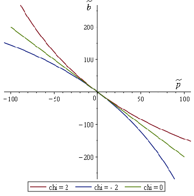
Figure 10: Comparison between expansions for the distinguished trajectories for $\varepsilon=10^{-5}$.

Note that by construction, setting $\chi=0$ reconstructs the trivial solution (29)–(32). Figure 10 compares the solutions in the $(b,p)$-plane for different values of $\chi$.

To demonstrate that each of the above expressions implies that the corresponding unscaled variable is a polynomial in $t$ and $\varepsilon$, consider for example the expansion for $\bar{z}=\delta^{6}\tilde{\bar{z}}$ in the case $\chi=1$ under the substitution $s=\varepsilon^{-2/3}t$ and $\delta=\varepsilon^{1/3}$. We have

$$\bar{z}(t,\varepsilon)=\delta^{6}\tilde{\bar{z}}(s,\delta)= \delta^{6}\left(-2-8s{\delta}^{2}+8{\delta}^{3}-24\,{s}^{2}{\delta}^{4}+48s{\delta}^{5}+\left(-\frac{368\,{s}^{3}}{5}+\frac{6672}{5}\right){\delta}^{6}+\mathcal{O}\left({\delta}^{7}\right)\right)$$

$$= \varepsilon^{2}\left(-2-8t+8\varepsilon-24t^{2}+48t\varepsilon+\left(-\frac{368\,{t}^{3}}{5\varepsilon^{2}}+\frac{6672}{5}\right)\varepsilon^{2}+\mathcal{O}\left({\delta}^{7}\right)\right)$$

$$= \varepsilon^{2}\left(-2-8t-24t^{2}-\frac{368}{5}t^{3}+(8+48t)\varepsilon+\frac{6672}{5}\varepsilon^{2}+\mathcal{O}(t^{4},\varepsilon t^{2},\varepsilon^{2}t,\varepsilon^{3})\right)$$

Note that the distinguished trajectory exists for both $t<0$ and $t>0$ and so can correspond to a canard solution that passes between the critical (slow) manifolds for $p<0$ and $p>0$. This solution can they play the role of the separatrix in the inner system that separates trajectories that lift off from those that take an IWC. To see whether this is the case, we have to consider other trajectories that are in the critical manifold for $p<0$. In order to do this we need to look at the outer scale and consider the asymptotic behaviour as $p\to 0$ of solutions in the slow manifold.

5.3 Fast-slow analysis of the outer system

Consider the general system (61)–(67). Letting $\varepsilon^{2}y_{o}=y$, $\varepsilon^{2}z_{o}=z$, $\varepsilon v_{o}=v$ gives

$$\dot{\xi} =F(\xi)+G(\xi)\lambda_{N},$$

$$\dot{p} =\alpha_{1}(\xi),$$

$$\dot{b} =\alpha_{2}(\xi)-\alpha_{3}(\xi)\lambda_{N},$$

$$\varepsilon\dot{y}_{o} =v_{o},$$

$$\varepsilon\dot{v}_{o} =b+p\lambda_{N},$$

$$\varepsilon\dot{z}_{o} =-z_{o}-\lambda_{N},$$

$$\lambda_{N} =z_{o}-y_{o}.$$

Note that this is a fast-slow system.

The fast system

is obtained by letting $\dot{\xi}=\dot{p}=\dot{b}=0$, in which case $\xi$, $p$ and $b$ are constant and we are left with a linear system for the remaining three variables

$$\varepsilon(\dot{y}_{o},\dot{v}_{o},\dot{z}_{o})^{T}=M(y_{o},v_{o},z_{o})^{T},$$

where

$$\mathbf{M}=\left[\begin{array}[]{ccc}0&1&0\\ -p&0&p\\ 1&0&-2\end{array}\right]$$

The characteristic polynomial of $M$ is

$$\lambda^{3}+2\lambda^{2}+p\lambda+p=0,$$

which is the same as that of the fast outer system in the motivating example, with the same conclusions regarding stability. Specifically, for $p>0$ trajectories are attracted to a codimension three manifold, representing the slow dynamics, whereas for $p<0$ the slow dynamics is normally hyperbolic with a two-dimensional stable manifold and one-dimensional unstable manifold.

The slow dynamics

for $\varepsilon=0$ occur on the slow manifold

$$y_{o} =2b/p,$$

$$v_{o} =0,$$

$$z_{o} =b/p,$$

whose dynamics are given by the slow subsystem

$$\dot{\xi} =F(\xi)-G(\xi)b/p,$$

$$\dot{p} =\alpha_{1}(\xi),$$

$$\dot{b} =\alpha_{2}(\xi)+\alpha_{3}(\xi)b/p.$$

Now, according to Fenichel theory (see [7]), for all $p$ bounded away from zero (where the slow manifold is normally-hyperbolic) then there exist a critical manifolds which are $O(\varepsilon)$ close to the slow manifold for $p>0$ and $p<0$, are smooth and inherent the stability properties of the slow manifold in each case.

In order to understand the limit as $p\to 0$ of the dynamics in the slow subsystem, it is useful to rewrite it in the form

$$\dot{\xi}-\left(F(\xi)+G(\xi)\lambda_{N}\right) =0,$$

$$\dot{p}-\alpha_{1}(\xi) =0,$$

$$\dot{b}-\left(\alpha_{2}(\xi)-\alpha_{3}(\xi)\lambda_{N}\right) =0,$$

$$-\left(b+p\lambda_{N}\right) =0.$$

We also write slow variables as deviations from the distinguished trajectory

$$\xi =\bar{\xi}(t,0)+\hat{\xi}(t),$$ (97)

$$p =\bar{p}(t,0)+\hat{p}(t),$$ (98)

$$b =\bar{b}(t,0)+\hat{b}(t),$$ (99)

$$\lambda_{N} =\bar{\lambda}_{N}(t,0)+\hat{\lambda}_{N}(t).$$ (100)

Motivatived by the example system in 4, we seek an ansatz of the form

$$\hat{\xi}(t) =\xi_{0}(-t)^{r}+o((-t)^{r}),$$ (101)

$$\hat{p}(t) =p_{0}(-t)^{r+1}+o((-t)^{r+1}),$$ (102)

$$\hat{b}(t) =b_{0}(-t)^{r}+o((-t)^{r})$$ (103)

$$\hat{\lambda}_{N}(t) =\lambda_{0}(-t)^{r-1}+o((-t)^{r-1}),$$ (104)

for an unknown exponent $r>0$, and using $\bar{p}(t,0)=\alpha_{1}^{*}t+\cdots$, we find to leading order that

$$\left[-r\xi_{0}-G^{*}\lambda_{0}\right](-t)^{r-1} =o((-t)^{r-1})$$ (105)

$$\left[-(r+1)p_{0}-{\alpha_{1}}_{\xi}^{*}\xi_{0}\right](-t)^{r} =o((-t)^{r})$$ (106)

$$\left[-rb_{0}+\alpha_{3}^{*}\lambda_{0}\right](-t)^{r-1} =o((-t)^{r-1})$$ (107)

$$\left[-b_{0}+\alpha_{1}^{*}\lambda_{0}\right](-t)^{r} =o((-t)^{r}).$$ (108)

From the last two equations, a solutions with $b_{0}\neq 0$ requires $r=\alpha_{3}^{*}/\alpha_{1}^{*}=\beta$. Then we find

$$\xi_{0} =-\frac{G^{*}}{\alpha_{3}^{*}}b_{0},$$ (109)

$$p_{0} =0,$$ (110)

$$\lambda_{0} =\frac{1}{\alpha_{1}^{*}}b_{0}.$$ (111)

Thus

$$b=\bar{b}(t,0)+b_{0}(-t)^{\beta}+o((-t)^{\beta}).$$ (112)

5.4 Matching the inner and outer solutions

The inner system is given by (72)–(78). There is a fast timescale $\delta$ (in $s$ time units). The fast dynamics is one-dimensional and $\tilde{z}$ evolves quickly to the slow manifold is $\tilde{z}=\tilde{y}/2$. The slow system becomes

$$\tilde{\xi}^{\prime} =\tilde{F}(\xi)+\tilde{G}(\xi)\lambda_{N}$$

$$\tilde{p}^{\prime} =\alpha_{1}(\xi)$$

$$\tilde{b}^{\prime} =\alpha_{2}(\xi)-\alpha_{3}(\xi)\lambda_{N}$$

$$\tilde{y}^{\prime} =\tilde{v}$$

$$\tilde{v}^{\prime} =\tilde{b}+\tilde{p}\lambda_{N},$$

with $\lambda_{N}=-\tilde{y}/2$.

Motivated by the preliminary simulations of Sec. 3.3, we will look for solutions (in the form of hatted variables) that are scaled deviations from the distinguished trajectory of the form

$$\tilde{p} =\tilde{\bar{p}}(s,\varepsilon^{1/3})$$

$$\tilde{b} =\tilde{\bar{b}}(s,\varepsilon^{1/3})+\varepsilon^{2(\beta-1)/3}\tilde{\hat{b}}(s)$$ (113)

$$\tilde{y} =\tilde{\bar{y}}(s,\varepsilon^{1/3})+\varepsilon^{(2(\beta-1)/3}\hat{y}(s)$$

$$\tilde{v} =\varepsilon^{4/3}\tilde{\bar{v}}(s,\varepsilon^{1/3})+\varepsilon^{(2(\beta-1)/3}\hat{v}(s).$$

Then, in the limit $\varepsilon\to 0$, to leading order in $\xi$, using the fact that $\tilde{\bar{p}}=\alpha_{1}^{*}s+\ldots$, we get

$$\hat{b}^{\prime} =\alpha_{3}^{*}\hat{y}/2,$$

$$\hat{y}^{\prime} =\hat{v},$$

$$\hat{v}^{\prime} =\hat{b}-\alpha_{1}^{*}s\hat{y}/2.$$

Elimination of $\hat{y}$ and $\hat{v}$ gives

$$\hat{b}^{\prime\prime\prime}+\frac{\alpha_{1}^{*}}{2}s\hat{b}^{\prime}-\frac{\alpha_{3}^{*}}{2}\hat{b}=0.$$

Rescaling time to $\tau=\kappa s$ with $\kappa=(-\alpha_{1}^{*}/2)^{1/3}$, we get precisely the same equation (56) that we obtained for perturbations to the distinguished trajectory for the as we obtained for the example system in Sec. 4 whose asymptotics are summarised in Appendix A. The rest of the analysis of the dynamics of this equation follows exactly as in Sec. 4.4. In particular, matching with the outer equation (112) shows that

$$\hat{b}(s)=b_{0}\kappa^{-\beta}\varepsilon^{2\beta/3}\Theta(\kappa s,\beta),$$

where the initial constant $b_{0}$ determines the sign of the perturbation from the distinguished trajectory. Thus, applying the results from the Appendix on the asymptotics of hypergeometric functions, we get the same conditions (60) that determine whether lift-off or IWC occur.

Moreover, the implications for the dynamics are precisely as discussed in Sec. 4.5.

6 Application to a frictional impact oscillator

We now apply the previously developed theory to a frictional impact oscillator proposed by [9], see also Fig. 1(b). Our goal here is to verify that the approximate solutions produced by the expansion scheme of Sec. 5 match the results of brute-force numerical simulation.

6.1 The system

The frictional impact oscillator consists of two point masses, two springs and two dampers. The mass $m_{1}$ is in unilateral contact with a moving belt with friction coefficient $\mu$. The system has two mechanical degrees of freedom and thus we use the generalized coordinates

$$q=\begin{pmatrix}\phi\\ \psi\end{pmatrix}$$

As [9] shows, its motion is governed by the equation

$$M(q)\ddot{q}=f(q,\dot{q})+Q_{N}(q)\lambda_{N}+Q_{T}\lambda_{T}$$

with

$$M(q) = \begin{pmatrix}m_{1}l^{2}&m_{1}l\sin(\phi)\\ m_{1}l\sin(\phi)&m_{1}+m_{2}\end{pmatrix},$$

$$f(q,\dot{q}) = \begin{pmatrix}-k_{\phi}(\phi-\phi_{0})-c_{\phi}\dot{\phi}-m_{1}gl\sin(\phi)\\ -k_{\psi}\psi-c_{\psi}\dot{\psi}-(m_{1}+m_{2})g-m_{1}l\cos(\phi)\dot{\phi}^{2}\end{pmatrix}$$

$$Q_{T}(q) = (\partial x/\partial q)^{T}=\begin{pmatrix}l\cos(\phi)\\ 0\end{pmatrix},$$

$$Q_{N}(q) = (\partial y/\partial q)^{T}=\begin{pmatrix}l\sin(\phi)\\ 1\end{pmatrix}$$

The horizontal and vertical position functions of the contact point are

$$x(q)=l\sin(\phi),\quad y(q)=\psi+l(1-\cos(\phi)).$$

Assuming positive slip, (i.e. $\lambda_{T}=-\mu\lambda_{N}$), these equations can be written in the form of (11) with

$$\xi=\begin{pmatrix}\phi\\ \psi\\ \dot{\phi}\\ \dot{\psi}\end{pmatrix},F=\begin{pmatrix}\xi_{3}\\ \xi_{4}\\ M^{-1}f\end{pmatrix},G=\begin{pmatrix}0\\ 0\\ M^{-1}(-Q_{N}+\mu Q_{T})\end{pmatrix}.$$

Using the procedure described in Sec. 2 we can derive expressions for $v$, $p$, $b$, $\alpha_{1}$, $\alpha_{2}$, and $\alpha_{3}$. These are given in Appendix B.

To study the behaviour near the singularity, we reduce the number of parameters by setting

$$m_{2} =m_{1},\qquad\mu=\frac{25}{12},\quad\phi_{0}=\phi^{*}+\frac{49}{20}-\frac{7}{12}\beta-\frac{9}{50}\kappa,$$

$$k_{\phi} =m_{1}gl,\quad c_{\phi}=0,\qquad k_{\psi}=\kappa\frac{m_{1}g}{l},\quad c_{\psi}=\frac{25}{108}(18-7\beta)m_{1}\sqrt{\frac{g}{l}}.$$

where the values of $m_{1}$, $g$ and $l$ determines a scale for mass, length, and time, but not have any other influence on the dynamics of the system. We leave the two parameters $\beta$ and $\kappa$ (of dimension 1) to be specified later.

The chosen values of $\mu$ and $\phi_{0}$ ensure that that we have the singularity at

$$\cos(\phi^{*}) =\frac{3}{5},\quad\sin(\phi^{*})=\frac{4}{5}\quad\dot{\phi}^{*}=-\sqrt{\frac{g}{l}}$$

$$\psi^{*} =-\frac{2}{5}l\quad\dot{\psi}^{*}=\frac{4}{5}\sqrt{gl}.$$

Furthermore we have

$$\alpha_{1}^{*} =-\frac{175}{408}\frac{1}{m_{1}}\sqrt{\frac{g}{l}},\qquad\alpha_{3}^{*}=-\frac{175}{408}\beta\frac{1}{m_{1}}\sqrt{\frac{g}{l}}$$

$$\alpha_{2}^{*} =\frac{30625\beta^{2}+9450\beta\kappa-61425\beta+8262\kappa-126765}{55080}g\sqrt{\frac{g}{l}}$$

which means that the quotient between $\alpha_{3}^{*}$ and $\alpha_{1}^{*}$ is equal to $\beta$ in accordance with (43), and the sign of $\alpha_{2}^{*}$ is controlled by $\kappa$. Hence, the frictional impact oscillator may belong to any of the classes I, II, and III, furthermore, $\beta$ may take any desired value.

6.2 Numerical verification in case III

For numerical simulations, we use units based on $m_{1}$, $l$, and $g$. By taking $\beta=7/3$, $\kappa=0$, we get $\alpha_{1}^{*}=-0.4289$, $\alpha_{2}^{*}=-1.8764$, and $\alpha_{3}^{*}=-1.0008$, which corresponds to case III. For contact smoothing, we use the compliant model of Sec. 2 with $\varepsilon=10^{-6}$. Two sets of initial conditions are tested: The angle coordinate is set to

$$\phi=\phi^{*}+0.1,\quad\dot{\phi}=-0.9\text{ or }\phi=\phi^{*}+0.1,\quad\dot{\phi}=-0.5$$

and the linear coordinate is set to be on just in contact $y=v=0$:

$$\psi=\cos(\phi)-1,\quad\dot{\psi}=-\sin(\phi)\dot{\phi}.$$

Relaxation of the $z$ dynamics was found to take about $10^{-3}$ time units, whereas the system was simulated for ${\cal O}(10^{-1})$ time units. Additionally, a third initial condition approximately on the distinguished trajectory at $p=0.01$ was chosen.

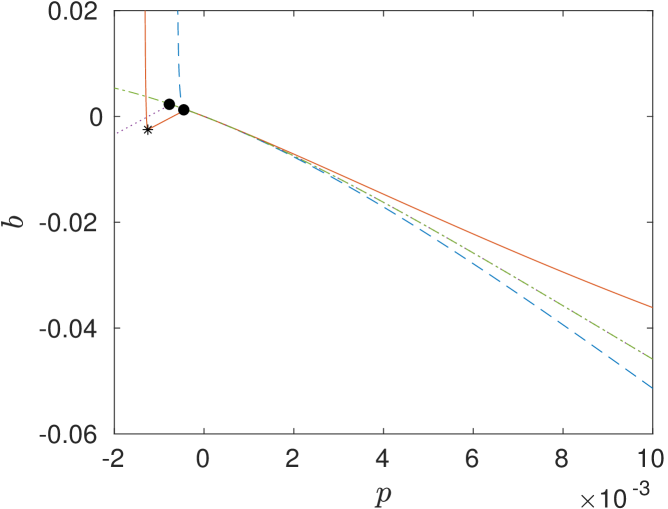
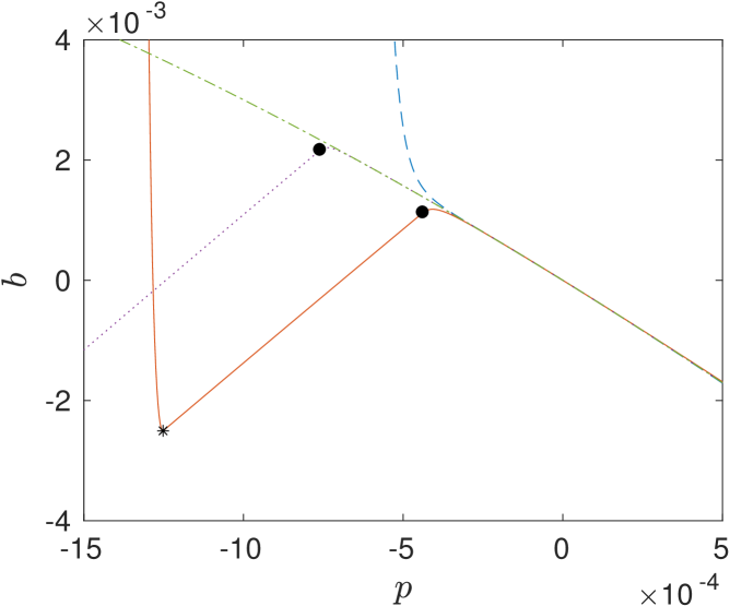
Figure 11: Numerical simulations of $p$ versus $b$ for the frictional impact oscillator with three different initial conditions (red/solid, blue/dashed, and purple/dotted curves), and asymptotic approximation of the distinguished trajectory (green/dash-dotted curve). Lift-off events are marked with a solid circle symbol, touch-down events with an asterisk symbol. The lower panel is a zoomed version of the same diagrams.

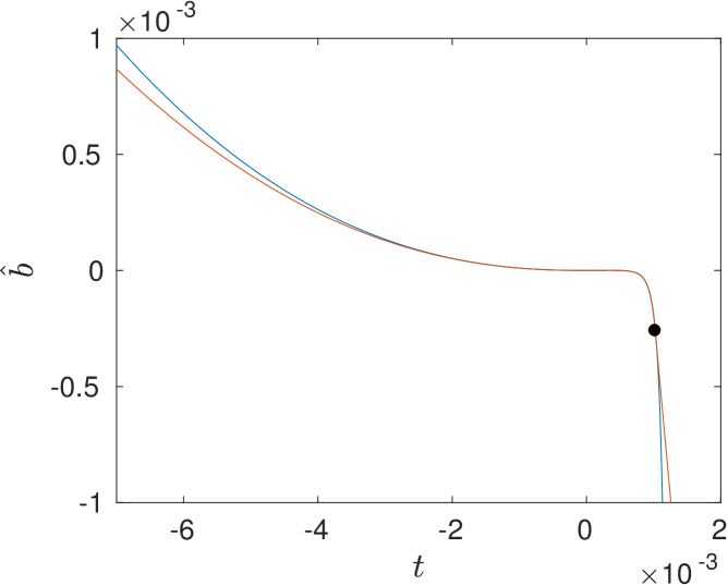
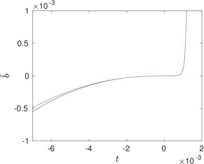
Figure 12: Diagrams of $\hat{b}$ versus time of the frictional impact oscillator for two initial conditions. The blue curves were obtained by numerical simulation, whereas the red curves are given by the suitable scaled $\Theta$ function.

Figure 11 shows a $p$ vs $b$ diagram. The red/solid curve (first initial condition) passes the (ghost) singularity, lifts off and then touches down again, initiating an “impact”. The blue/dashed curve (second initial condition) goes directly to an ”impact”. The purple/dotted curve is the trajectory using an initial condition approximately on the distinguished trajectory, and the green/dash-dotted curve is the appoximate distinguished trajectory itself, computed from the power series with $M=15$. These two are indistinguishable for $p>0$, but although the purple/dotted curve is able to follow the distinguished trajectory further into $p<0$ than the other initial conditions, it still eventually deviates. In all, these results are consistent with our finding that the distinguished trajectory is on a separatarix.

Figure 12(a) shows a diagram of the deviation $\hat{b}$ (see (113)) from the distinguished trajectory versus $t$. The time origin is shifted to make $p=0$ at $t=0$. The red curve is simulation using the first initial condition. The blue curve is computed using the suitably scaled hypergeometric $\Theta$ function, where time scale is based on $\alpha_{1}^{*}$, and the amplitude scale is adjusted to make the curves coincide when $t=0$. Lift-off in the simulation takes place just after $t=10^{-3}$, explaining the fast-growing deviation between the two curves for more positive times, since the hypergeometric solution assumes contact. At the same time, the deviation for negative times grows more slowly, and it is a natural consequence of the approximations used when developing the inner system. Figure 12(b) shows the same thing for the second initial condition. In this case there is no loss of contact, and the two curves fit each other very well for positive times.

7 Conclusion

The analysis in this paper provides a key step in the resolution of one of the simplest consequences of the paradox on the inconsistency of rigid body mechanics subject to Coulomb frication, first described by Painlevé in 1895 [14]. Despite numerous treatments in the intervening 120 years or so, as pointed out in [1], there remain many unsolved problems. Even for planar configurations with a single frictional point contact, it was previsouly known that open sets of initial conditions can approach the finite-time singularity that is known as dynamic jam, represented by the G-spot. What we have established in this paper is a general method for establishing what happens beyond the G-spot, at least in theory, and also understanding the sensitivity of what is observed to any smoothing through contact regularisation.

There are several weakness to the analysis we have presented. First, we have been unable to resolve in general what happens beyond the first lift-off or onset of IWC. Not only is there extreme sensitivity because during an IWC, but lift-off occurs with vanishingly small free normal acceleration as $\varepsilon\to 0$. In cases III and I this would occur with $\dot{b}<0$ so that lift-off would lead rapidly to further impact with small normal velocity. Whether this impact would again lead to further lift off close to the G-spot is unclear in general. It is conceivable that in the limit $\varepsilon\to 0$ one might have an infinite sequence of impacts with which might accumulate either in forward time (chatter) or in reverse time (reverse chatter). The latter would represent a point of infinite indeterminancy, as analysed in [11]. Further analysis of the dynamics post the first lift-off will form the subject of future work.

A second weakness is a lack of rigour. While we have formulated the existence of the distinguished trajectory as a Theorem, in general our analysis is asymptotic in nature. There is also a frustrating lack of a proof in cases where we have identified that an IWC probably occurs, because we cannot rule out the possibility of a lift-off in certain pathological examples. In particular, even though the asymptotics indicate a trajectory for which $\tilde{\hat{y}}$ diverges to $-\infty$ for large $s>0$ and $\tilde{\hat{y}}\ll 0$ for $s=0$, this is not sufficient to show that $\tilde{\hat{y}}$ remains negative for all $s>0$. Numerical results indicate that an impact always occurs. Perhaps further study of the appropriate generalised hypergeometric functions will shed further light on this question. During the final preparation of this manuscript we also become aware of the independent work of Hogan & Kristiansen [5] which studies a similar problem to the one considered here. They use completely different methods, namely geometric singular perturbation theory, to establish the existence of a canard trajectory. It is probable that a combination of their analysis with the asympotitic analysis conducted here would lead to some more comprehensive results.

A third weakness is the lack of experimental work to confirm what might happen in practice. In fact, while there have been several practical observations of the consequences of the Painlevé paradox (see [1]), we are not aware of any detailed quantitative experimental studies. One of the difficulties here is that dynamic jam represents a point of extreme sensitivity in the dynamics, therefore what is observed is likely to be highly dependent on the precise details of any imperfections or asperities in any practical model. Nevertheless, it would seem to be high time for the design of a detailed test rig to demonstrate each of cases I to III illustrated here.

Finally we should point out that the problem studied here is rather idealised. In practice, no structure ever undergoes point contact per se, there is always some form of regional contact. As shown in [16] the dynamics of systems with multiple point contacts can be much more complex, with various novel forms of Painlevé paradox that involve interaction between simultaneous contacts. Also, as demonstrated in [1][Sec. 7], there is yet more complexity if we study fully three-dimensional dynamics. For example, for certain configurations it is possible to enter the Painlevé region $p<0$ without passing through a neighbourhood of the G-spot.

There are clearly many situations that require further analysis along the lines developed in this paper.

Acknowledgements

This work was initiated at the Centre Recherca Matemàtica (CRM) Barcelona during the three-month programme in 2016 on Nonsmooth Dynamical Systems. The authors thank the CRM for its support, and especially Mike Jeffrey and Thibaut Putelat for useful discussion. Preliminary ideas for this paper were developed in collaboration with Harry Dankowicz, whose insights we also gratefully acknowledge. We are also grateful to Kristian Kristiansen and John Hogan for sharing their unpublished independent work with us at the latter stages of preparation of this paper. PLV acknowledges support from the National Research, Innovation and Development Office of Hungary under grant K104501 and ARC from the UK EPSRC under Programme Grant “Engineering Nonlinearity” EP/K003836/2.

Appendix A Generalised hypergeometric functions and their large time asymptotics

Consider the following third-order non-autonomous equation

$$\frac{d^{3}}{d\tau^{3}}\theta-\tau\frac{d}{d\tau}\theta+\beta\theta=0.$$ (A.1)

The solutions to this equation can be expressed in terms of generalised hypergeometric functions. In particular, by standard results, see e.g. [12, Ch.16], we have the following result.

Theorem 4.

The general solution of the differential equation (A.1) can be expressed as

$$\theta(\tau)=\theta(0)\>{}_{1}F_{2}\left(-\frac{\beta}{3};\frac{1}{3},\frac{2}{3};\frac{\tau^{3}}{9}\right)+\frac{d}{d\tau}\theta(0)\tau\>{}_{1}F_{2}\left(\frac{1}{3}-\frac{\beta}{3};\frac{2}{3},\frac{4}{3};\frac{\tau^{3}}{9}\right)+\frac{d^{2}}{d\tau^{2}}\theta(0)\frac{\tau^{2}}{2}\>{}_{1}F_{2}\left(\frac{2}{3}-\frac{\beta}{3};\frac{4}{3},\frac{5}{3};\frac{\tau^{3}}{9}\right).$$

where ${}_{1}F_{2}$ is the generalised hypergeometric function with indices $[1,2]$.

We are interested in the asympotics of this solution as $|\tau|\to\infty$. Using the general asymptotic expansion of ${}_{1}F_{2}$ for complex arguments in the limit of large $|\tau|$, we can formulate the following results.

Theorem 5 (Asymptotics of ${}_{1}F_{2}$ for large negative $\tau$).

Define $h$ as a formal series

$$h(\tau,\beta)=3^{\beta/3-1}(-\tau)^{\beta}\sum_{k=0}^{\infty}\frac{1}{k!3^{k}(-\tau)^{3k}\Gamma(1+\beta-3k)}$$ (A.2)

and $e_{r}$, $e_{i}$ as the real and imaginary parts of the formal series

$$e_{r}(\tau,\beta)+ie_{i}(\tau,\beta)=\sqrt{\pi}3^{\beta/3-1}(-\tau)^{-\beta/2-3/4}e^{i(\pi\beta/6+\pi/4-2(-\tau)^{3/2}/3)}\sum_{k=0}^{\infty}\frac{c_{k}(\beta)i^{k}3^{k}}{2^{k}(-\tau)^{3k/2}}.$$ (A.3)

Here the coefficients $c_{k}$ are determined via a somewhat complicated recurrence relation, see [12, Eq.16.11.4]. In particular, we have

$$c_{0}=1.$$ (A.4)

Then, provided $\beta$ is not an integer, asymptotically, as $\tau\rightarrow-\infty$

$${}_{1}F_{2}\left(-\frac{\beta}{3};\frac{1}{3},\frac{2}{3};\frac{\tau^{3}}{9}\right)\sim 3\Gamma\left(\frac{3+\beta}{3}\right)h(\tau,\beta)+\frac{3}{\Gamma\left(-\frac{\beta}{3}\right)}2e_{r}(\tau,\beta),$$ (A.5)

$$\tau\>{}_{1}F_{2}\left(\frac{1}{3}-\frac{\beta}{3};\frac{2}{3},\frac{4}{3};\frac{\tau^{3}}{9}\right),\sim-3^{2/3}\Gamma\left(\frac{2+\beta}{3}\right)h(\tau,\beta)-\frac{3^{2/3}}{\Gamma\left(\frac{1-\beta}{3}\right)}\left(e_{r}(\tau,\beta)-\sqrt{3}e_{i}(\tau,\beta)\right),$$ (A.6)

$$\frac{\tau^{2}}{2}\>{}_{1}F_{2}\left(\frac{2}{3}-\frac{\beta}{3};\frac{4}{3},\frac{5}{3};\frac{\tau^{3}}{9}\right),\sim 3^{1/3}\Gamma\left(\frac{1+\beta}{3}\right)h(\tau,\beta)+\frac{3^{1/3}}{\Gamma\left(\frac{2-\beta}{3}\right)}\left(-e_{r}(\tau,\beta)-\sqrt{3}e_{i}(\tau,\beta)\right).$$ (A.7)

We want to choose the specific solution $\theta(\tau)=\Theta(\tau)$ whose initial conditions are such that the coefficients of the highly oscillatory terms $e_{r}$ and $e_{i}$ vanish. The remaining $h$ term is dominated by its first term, which is proportional to $(-\tau)^{\beta}$. In particular, using the particular initial conditions

$$\Theta(0) = \frac{\Gamma\left(\frac{-\beta}{3}\right)}{3^{(3+\beta)/3}\Gamma(-\beta)},$$ (A.8)

$$\frac{d\Theta}{d\tau}(0) = \frac{\Gamma\left(\frac{1-\beta}{3}\right)}{3^{(2+\beta)/3}\Gamma(-\beta)},$$ (A.9)

$$\frac{d^{2}\Theta}{d\tau^{2}}(0) = \frac{\Gamma\left(\frac{2-\beta}{3}\right)}{3^{(1+\beta)/3}\Gamma(-\beta)},$$ (A.10)

we define a function $\Theta$ with the asymptotic behaviour

$$\Theta(\tau,\beta)\sim 3^{1-\beta/3}\Gamma\left(1+\beta\right)h(\tau,\beta)\sim(-\tau)^{\beta}$$

as $\tau\rightarrow-\infty$.

Theorem 6 (Asymptotic of ${}_{1}F_{2}$ for large positive $\tau$).

Define $e_{1}$ as the formal series

$$e_{1}(\tau,\beta)=\sqrt{\pi}3^{\beta/3-1}(\tau)^{-\beta/2-3/4}e^{2\tau^{3/2}/3}\sum_{k=0}^{\infty}\frac{c_{k}(\beta)3^{k}}{2^{k}(\tau)^{3k/2}}.$$

where the $c_{k}$ coefficients are defined as in the previous theorem. Then asymptotically, as $\tau\rightarrow\infty$,

$${}_{1}F_{2}\left(-\frac{\beta}{3};\frac{1}{3},\frac{2}{3};\frac{\tau^{3}}{9}\right)\sim\frac{3}{\Gamma\left(-\frac{\beta}{3}\right)}e_{1}(\tau,\beta)$$ (A.11)

$$\tau\>{}_{1}F_{2}\left(\frac{1}{3}-\frac{\beta}{3};\frac{2}{3},\frac{4}{3};\frac{\tau^{3}}{9}\right)\sim\frac{3^{2/3}}{\Gamma\left(\frac{1-\beta}{3}\right)}e_{1}(\tau,\beta)$$ (A.12)

$$\frac{\tau^{2}}{2}\>{}_{1}F_{2}\left(\frac{2}{3}-\frac{\beta}{3};\frac{4}{3},\frac{5}{3};\frac{\tau^{3}}{9}\right)\sim\frac{3^{1/3}}{\Gamma\left(\frac{2-\beta}{3}\right)}e_{1}(\tau,\beta)$$ (A.13)

Applied to the $\Theta$ functions this means

$$\Theta(\tau,\beta)\sim\frac{3^{1-\beta/3}}{\Gamma(-\beta)}e_{1}(\tau,\beta)\sim\frac{\sqrt{\pi}}{\Gamma(-\beta)}\exp((2/3)\tau^{3/2})(\tau)^{-\beta/2-3/4}$$ (A.14)

as $\tau\rightarrow\infty$, where we have used $c_{0}=1$.

Appendix B Expressions for the frictional impact oscillator

$$v(\phi,\psi,\dot{\phi},\dot{\psi})=\dot{\psi}+l\sin(\phi)\dot{\phi}$$

$$p(\phi,\psi)=\frac{m_{1}\cos(\phi)^{2}+m_{2}\sin(\phi)(\sin(\phi)-\mu\cos(\phi))}{m_{1}(m_{2}+m_{1}\cos(\phi)^{2})}$$

$$b(\phi,\psi,\dot{\phi},\dot{\psi})=\frac{m_{1}l\cos(\phi)\left(m_{2}l\dot{\phi}^{2}-\cos(\phi)(k_{\psi}\psi+c_{\psi}\dot{\psi})\right)-m_{2}\sin(\phi)(k_{\phi}(\phi-\phi_{0})+c_{\phi}\dot{\phi})}{m_{1}l(m_{2}+m_{1}\cos(\phi)^{2})}-g$$

$$\alpha_{1}(\phi,\psi,\dot{\phi},\dot{\psi})=-\frac{m_{2}\left(\mu\left(\cos(\phi)^{2}\left(m_{1}+2m_{2}\right)-m_{2}\right)-2m_{2}\sin(\phi)\cos(\phi)\right)}{m_{1}\left(m_{2}+m_{1}\cos(\phi)^{2}\right)^{2}}\dot{\phi}$$

$$\alpha_{2}(\phi,\psi,\dot{\phi},\dot{\psi})=\frac{1}{m_{1}^{2}l^{3}\left(m_{2}+m_{1}\cos(\phi)^{2}\right)^{2}}\left[m_{1}^{2}\left(m_{2}+m_{1}\cos(\phi)^{2}\right){l}^{3}gc_{\psi}\cos(\phi)^{2}\right.\\ -m_{1}^{2}\left(m_{2}+m_{1}\cos(\phi)^{2}\right){l}^{3}k_{\psi}\cos(\phi)^{2}\dot{\psi}+m_{1}^{3}{l}^{4}c_{\psi}\cos(\phi)^{3}{\dot{\phi}}^{2}-m_{1}^{2}{l}^{2}c_{\psi}\cos(\phi)^{2}\sin(\phi)\left(k_{\phi}\left(\phi-\phi_{0}\right)+c_{\phi}\dot{\phi}\right)\\ +m_{1}^{2}{l}^{3}c_{\psi}\cos(\phi)^{2}\left(k_{\psi}\psi+c_{\psi}\dot{\psi}\right)-m_{1}m_{2}lc_{\phi}\sin(\phi)^{2}\left(k_{\psi}\psi+c_{\psi}\dot{\psi}\right)\\ -m_{1}^{2}m_{2}{l}^{2}c_{\phi}\cos(\phi)\sin(\phi)^{2}\dot{\phi}^{2}-m_{1}^{2}m_{2}^{2}{l}^{4}\sin(\phi)\dot{\phi}^{3}+m_{2}\left(m_{1}+m_{2}\right)c_{\phi}\sin(\phi)\left(k_{\phi}\left(\phi-\phi_{0}\right)+c_{\phi}\dot{\phi}\right)\\ +4m_{1}^{2}m_{2}{l}^{3}\cos(\phi)\sin(\phi)\dot{\phi}\left(k_{\psi}\psi+c_{\psi}\dot{\psi}\right)-3m_{1}m_{2}^{2}{l}^{2}\cos(\phi)\dot{\phi}\left(k_{\phi}\left(\phi-\phi_{0}\right)+c_{\phi}\dot{\phi}\right)\\ +3m_{1}^{3}m_{2}{l}^{4}\cos(\phi)^{2}\sin(\phi)\dot{\phi}^{3}+m_{1}^{2}m_{2}{l}^{2}\cos(\phi)^{3}\dot{\phi}\left(k_{\phi}\left(\phi-\phi_{0}\right))+c_{\phi}\dot{\phi}\right)\\ \left.-m_{1}m_{2}\left(m_{2}+m_{1}\cos(\phi)^{2}\right){l}^{2}k_{\phi}\sin(\phi)\dot{\phi}-4m_{1}^{2}m_{2}{l}^{2}\cos(\phi)\dot{\phi}\left(k_{\phi}\left(\phi-\phi_{0}\right)+c_{\phi}\dot{\phi}\right)\right]$$

$$\alpha_{3}(\phi,\psi,\dot{\phi},\dot{\psi})=\frac{1}{m_{1}^{2}l^{2}\left(m_{2}+m_{1}\cos(\phi)^{2}\right)^{2}}\left[m_{1}^{2}l^{2}c_{\psi}\cos(\phi)^{3}\left(\mu\sin(\phi)+\cos(\phi)\right)\right.\\ +2m_{1}^{2}m_{2}l^{2}\mu\cos(\phi)^{2}\dot{\phi}+2m_{1}m_{2}^{2}l^{2}\cos(\phi)\left(\mu\cos(\phi)-\sin(\phi)\right)\dot{\phi}\\ \left.-m_{2}(m_{1}+m_{2})c_{\phi}\mu\cos(\phi)\sin(\phi)+m_{2}^{2}c_{\phi}\sin(\phi)^{2}\right]$$

References

- [1] A.R. Champneys and P.L. Várkonyi. The painlevé paradox in contact mechanics. IMA Journal of Applied Mathematics, 81:538–588, 2016.
- [2] A. Chatterjee and A. Ruina. A new algebraic rigid-body collision law based on impulse space considerations. ASME Journal of Applied Mechanics, 65:939–951, 1998.
- [3] F. Génot and B. Brogliato. New results on Painlevé paradoxes. European Journal of Mechanics A/Solids, 18:653–677, 1999.
- [4] G. Haller and S. Ponsion. Nonlinear normal modes and spectral submanifolds: Existence, uniqueness and use in model reduction, 2016. arXiv:1602.00560v2.
- [5] S.J. Hogan and K.U. Kristiansen. Personal communication, 2016. Unpublished notes.
- [6] S.J. Hogan and K.U. Kristiansen. Regularization of impact with collision: the Painleé paradox and compliance, 2016. Preprint: arxiv.org/pdf/1610.00143 .
- [7] C. Kuhn. Multiple timescale dynamical systems. Springer-Verlag, Berlin, 2015.
- [8] R.I. Leine, B. Brogliato, and H. Nijmeijer. Periodic motion and bifurcations induced by the Painlevé paradox. European Journal of Mechanics A/Solids, 21:869–896, 2002.
- [9] R.I. Leine and N van de Wouw. Stability properties of equilibrium sets of non-linear mechanical systems with dry friction and impact. Nonlinear Dynamics, 51(4):551–583, 2008.
- [10] A. Nordmark, H. Dankowicz, and Champneys A. Discontinuity-induced bifurcations in systems with impacts and friction: Discontinuities in the impact law. Int. J. Nonlinear Mech., 44:1011–1023, 2009.
- [11] A. Nordmark, H. Dankowicz, and A. Champneys. Friction-induced reverse chatter in rigid-body mechanisms with impacts. IMA Journal of Applied Mathematics, 76:85–119, 2011.
- [12] F.W.J. Olver, Lozier D.W., R.F. Boisvert, and C.W Clark. The NIST Handbook of Mathematical Functions. Cambridge Univeristy Press, Cambridge, 2010.
- [13] Y. Or and E. Rimon. Investigation of Painlevé’s paradox and dynamic jamming during mechanism sliding motion. Nonlinear Dyn., 67:1647–1668, 2012.
- [14] P. Painlevé. Sur les lois du frottement de glissement. Comptes Rendu des Séances de l’Académie des Sciences, 121:112–115, 1895.
- [15] W.J. Stronge. Impact Mechanics. Cambridge University Press, Cambridge, UK, 2000.
- [16] P.L. Várkonyi. Dynamics of mechanical systems with two sliding contacts: new facets of painlevé’s paradox. Archive of Applied Mechanics, DOI: 10.1007/s00419-016-1165-1, 2016.