Robust Detection of Random Events with Spatially Correlated Data in Wireless Sensor Networks via Distributed Compressive Sensing

Abstract

In this paper, we exploit the theory of compressive sensing to perform detection of a random source in a dense sensor network. When the sensors are densely deployed, observations at adjacent sensors are highly correlated while those corresponding to distant sensors are less correlated. Thus, the covariance matrix of the concatenated observation vector of all the sensors at any given time can be sparse where the sparse structure depends on the network topology and the correlation model. Exploiting the sparsity structure of the covariance matrix, we develop a robust nonparametric detector to detect the presence of the random event using a compressed version of the data collected at the distributed nodes. We employ the multiple access channel (MAC) model with distributed random projections for sensors to transmit observations so that a compressed version of the observations is available at the fusion center. Detection is performed by constructing a decision statistic based on the covariance information of uncompressed data which is estimated using compressed data. The proposed approach does not require any knowledge of the noise parameter to set the threshold, and is also robust when the distributed random projection matrices become sparse.

Keywords: Compressive sensing, random events, detection theory, statistical dependence, wireless sensor networks

I Introduction

Over the last two decades, wireless sensor network (WSN) technology has gained increasing attention by both research community and actual users [1, 2, 3, 4, 5, 6, 7, 8]. Sensor networks are inherently resource constrained and they starve for energy and communication efficient protocols [1]. There is abundant literature related to energy-saving in WSNs as numerous methods have been proposed for energy efficient protocols in the last several years. However, there is still much ongoing research on how to optimize power and communication bandwidth in resource constrained sensor networks since none of the existing standalone protocol is universally applicable.

Recent advances in compressive sensing (CS) have led to novel approaches to design energy efficient WSNs. Sparsity is a common characteristic that can be observed in WSN applications in various forms. For example, in many applications, the time samples collected at a given node can be represented in a sparse manner in a given basis [9]. When considering multiple measurement vectors (MMVs) collected at distributed nodes, different sparsity patterns with certain structures can be observed [9]. Joint processing of such MMVs using CS techniques by exploiting temporal sparsity along with different joint structures leads to energy efficient signal processing as desired by WSNs. Spatial sparsity of observations collected at distributed nodes is another form of sparsity. For example, since not all the sensors gather informative observations at any given time, to make a compressed version of the observations available at the fusion center, random projections can be employed [10]. Spatial sparsity can also be leveraged by construction such as in source localization and sparse event detection [11, 12, 13]. In addition to complete signal reconstruction as is commonly done in the CS literature, CS has been exploited for detection problems exploiting temporal, or spatial spatial sparsity [14, 15, 16, 17, 18, 19] or without exploiting any sparsity prior of signals [20, 21, 22, 23].

In contrast to these existing works, in this paper, our goal is to exploit the sparsity or structural properties of the covariance matrix of spatially correlated data (but not sparsity of observations itself) to solve a random event detection problem. In particular, a decision statistic is computed using the covariance information of data collected at multiple sensors. In a typical WSN, the densely deployed sensor observations can be highly correlated. In [24, 25], several spatial correlation models have been discussed. With most of these models, the correlation among nodes that are located far from each other is negligible. Thus, the covariance matrix of the concatenated data vector can have a sparse or some known structure which is determined by the spatial correlation model and the network topology. If only a compressed version of the concatenated data vector is received at the fusion center, the covariance matrix can be computed based on compressed data as considered in compressive covariance sensing [26]. To have a compressed version of spatially correlated data at the fusion center, we employ the multiple access channel (MAC) model with distributed random projections [10, 27]. Using the sample estimate of the covariance matrix of compressed data with limited samples, we compute a decision statistic in terms of the covariance matrix of uncompressed data. The proposed approach does not require any knowledge of the noise parameters for threshold setting as needed by likelihood ratio (LR) based and/or energy detectors. Further, the proposed approach is shown to be robust to the selection of the distributed projection matrices (i.e., dense vs sparse matrices).

This work is motivated by our recent work in [28], in which a similar decision statistic was computed to perform detection with multi-modal (non-Gaussian in general) dependent data in the compressed domain. However, the application scenario and the problem formulation in this work are different from that in [28] mainly with respect to the compression model used at each sensor and the communication architecture between the sensors and the fusion center.

II Detection with Spatially Correlated Data in WSNs

Let there be $L$ sensor nodes in a network deployed to solve a binary hypothesis testing problem where the two hypotheses are denoted by $\mathcal{H}_{1}$ (signal present) and $\mathcal{H}_{0}$ (signal absent). Consider the detection of a random signal, denoted by $S$, emitted by a point source. The $n$-th measurement at the $j$-th node is denoted by $x_{nj}$ for $j=1,\cdots,L$ and $n=1,\cdots,T$. Under the two hypotheses, $x_{nj}$ is given by.

$$\mathcal{H}_{1} : x_{nj}=s_{nj}+v_{nj}$$

$$\mathcal{H}_{0} : x_{nj}=v_{nj}$$ (1)

for $j=1,\cdots,L$ and $n=1,\cdots,T$, where $s_{nj}$ is the realization of $S$ at the $j$-th node at time $n$, $v_{nj}\sim\mathcal{N}(0,\sigma_{v}^{2})$ is the noise which is assumed to be Gaussian and iid over $j$ and $n$. We further define $\mathbf{x}[n]=[x_{n1},\cdots,x_{nL}]^{T}$ to be the observation vector over all the nodes at time $n$. Similarly, we use the notations $\mathbf{s}[n]$ and $\mathbf{v}[n]$, respectively, to denote the signal and noise vectors at time $n$. The mean and the variance of $S$ are denoted by $\mu_{S}$ and $\sigma_{S}^{2}$, respectively. Without loss of generality, we assume that $\mu_{S}=0$.

In a dense sensor network where the nodes are located very close to each other, the elements of $\mathbf{s}[n]$ can be correlated at any given time when all the nodes observe the same random phenomenon. Let the covariance matrix of $\mathbf{s}[n]$ be denoted by $\bm{\Sigma}_{s}$ with the $(i,j)$-th element, $\bm{\Sigma}_{s}[i,j]=\rho_{ij}\sigma_{S}^{2}$ for $i\neq j$. We define $\rho_{ij}$ to be the correlation coefficient between $s_{ni}$ and $s_{nj}$ which is given by

$$\rho_{ij}=\frac{\mathrm{cov}(s_{ni},s_{nj})}{\sigma_{S}^{2}}.$$ (2)

In [24], several spatial correlation models were discussed in which $\rho_{ij}$ is expressed as $\rho_{ij}=G_{\vartheta}(r_{ij})$ where $r_{ij}$ denotes the distance between the $i$-th node and the $j$-th node, and $G_{\vartheta}(\cdot)$ defines the correlation model (e.g., spherical, power exponential, etc..). If $S$ is assumed to be Gaussian and $\bm{\Sigma}_{s}$ and $\sigma_{v}^{2}$ are known, the LR test can be employed to solve the detection problem (1) assuming that $\mathbf{x}[n]$ for $n=1,\cdots,T$ is available at a central fusion center. However, when these parameters are unknown and/or $S$ is not Gaussian, performing LR based detection is challenging. In such scenarios, one of the commonly used nonparametric detectors is the energy detector. While the energy detector shows good performance when $S$ is Gaussian, its susceptibility to the exact knowledge of the noise power makes the energy detector not very attractive in many practical settings. Further, making $\mathbf{x}[n]$ available at the fusion center may require considerable communication overhead which can be undesirable in resource constrained sensor networks.

To address these issues, we exploit CS theory to make a compressed version of $\mathbf{x}[n]$ available at the fusion center and propose a robust nonparametric detector based on covariance information of the uncompressed observations. When the random event is present, the covariance matrix of $\mathbf{x}[n]$ is non-diagonal while it is diagonal in the presence of only noise. Thus, a decision statistic based on the covariance matrix of $\mathbf{x}[n]$ can be used to perform detection. On the other hand, based on most of the spatial correlation models discussed in [24], the observations at nearby sensors are strongly correlated while the correlation reduces as the distance between nodes increases. Thus, $\bm{\Sigma}_{s}$ can be assumed to have a sparse structure. If a compressed version of $\mathbf{x}[n]$ is available at the fusion enter, the concepts of CS can be utilized to construct a decision statistic based on $\bm{\Sigma}_{s}$ without having access to the raw observations $\mathbf{x}[n]$.

III Nonparametric Compressed Detection of a Random Event via MAC

To obtain a compressed version of $\mathbf{x}[n]$ at the fusion center, we employ the MAC architecture as proposed in [10, 27]. In the MAC model, the $j$-th node multiplies its observation at time $n$ by a scalar quantity denoted by $\mathbf{A}[i,j]$ and transmits it coherently so that the fusion center receives,

$$y_{ni}=\sum_{j=1}^{L}\mathbf{A}[i,j]\mathbf{x}_{nj}+w_{ni}$$ (3)

with the $i$-th transmission where $w_{ni}\sim\mathcal{N}(0,\sigma_{w}^{2})$ is the noise at the fusion center which is assumed to be Gaussian and iid. The observed signal vector at the fusion center at time $n$ after $M$ transmissions can be expressed as $\mathbf{y}[n]=\mathbf{A}\mathbf{x}[n]+\mathbf{w}[n]$ where $\mathbf{A}\in\mathbb{R}^{M\times N}$, and $\mathbf{w}[n]\sim\mathcal{N}(\mathbf{0},\sigma_{w}^{2}\mathbf{I})$ with $\mathbf{I}$ denoting the identity matrix. With this model, the detection problem reduces to,

$$\mathcal{H}_{1}:~{}\mathbf{y}[n] = \mathbf{A}\mathbf{s}[n]+\tilde{\mathbf{w}}[n]$$

$$\mathcal{H}_{0}:~{}\mathbf{y}[n] = \tilde{\mathbf{w}}[n]$$ (4)

where $\tilde{\mathbf{w}}[n]=\mathbf{A}\mathbf{v}[n]+\mathbf{w}[n]$. In the rest of the paper, we assume that the elements of $\mathbf{A}$ are zero mean random and satisfy $\mathbf{A}\mathbf{A}^{T}=\mathbf{I}$ (we discuss the robustness of the proposed method when this condition is relaxed in Section IV). Then, we have $\tilde{\mathbf{w}}[n]\sim\mathcal{N}(\mathbf{0},\sigma_{\tilde{w}}^{2}\mathbf{I})$ where $\sigma_{\tilde{w}}^{2}=\sigma_{v}^{2}+\sigma_{w}^{2}$. Let $\bm{\Sigma}_{y}=\mathbb{E}\{\mathbf{y}[n]\mathbf{y}[n]^{T}\}$ denote the covariance matrix of $\mathbf{y}[n]$ which is given by $\bm{\Sigma}_{y}=\mathbf{A}\tilde{\bm{\Sigma}}_{x}\mathbf{A}^{T}$ where

$$\tilde{\bm{\Sigma}}_{x}=\left\{\begin{array}[]{ccc}\bm{\Sigma}_{s}+\sigma_{\tilde{w}}^{2}\mathbf{I}\triangleq\tilde{\bm{\Sigma}}_{s}{}&\mathrm{under}~{}\mathcal{H}_{1}\\ \sigma_{\tilde{w}}^{2}\mathbf{I}{}&\mathrm{under}~{}\mathcal{H}_{0}\end{array}\right..$$ (7)

It is noted that $\tilde{\bm{\Sigma}}_{x}$ is the covariance matrix of $\mathbf{x}[n]$ if $\mathbf{x}[n]$ was available at the fusion center in the presence of noise with mean zero and the covariance matrix $\sigma_{w}^{2}\mathbf{I}$.

The goal is to decide as to which hypothesis is true based on (4) when the signal and noise statistics are completely unknown at the fusion center. From (7), it is seen that $\tilde{\bm{\Sigma}}_{x}$ has different structures under the two hypotheses which can be used to construct a decision statistic. Here we consider the following decision statistics based on $\tilde{\bm{\Sigma}}_{x}$ [28, 29, 30]:

$$\Lambda_{C}=\frac{\underset{i,j}{\sum}|\tilde{\bm{\Sigma}}_{x}[i,j]|}{\underset{i}{\sum}|\tilde{\bm{\Sigma}}_{x}[i,i]|}$$ (8)

where $|\cdot|$ denotes the absolute value. Note that $\bm{\Sigma}_{y}$ is a compressed version of $\tilde{\bm{\Sigma}}_{x}$ where $\tilde{\bm{\Sigma}}_{x}$ has a sparse structure under $\mathcal{H}_{1}$ with different correlation models as discussed in [24]. This motivates us to exploit the concepts of compressive covariance sensing [26] to efficiently compute $\Lambda_{C}$ based on $\bm{\Sigma}_{y}$. In this paper, we replace $\bm{\Sigma}_{y}$ by its sample estimate, $\tilde{\bm{\Sigma}}_{y}$, which is given by, $\tilde{\bm{\Sigma}}_{y}=\frac{1}{T}\sum_{n=1}^{T}\mathbf{y}[n]\mathbf{y}[n]^{T}$.

III-A Computation of $\Lambda_{C}$

The specific procedure to estimate $\tilde{\bm{\Sigma}}_{x}$ from $\tilde{\bm{\Sigma}}_{y}$ depends on the structure of $\tilde{\bm{\Sigma}}_{x}$ which depends on the sensor network configuration and the correlation model. Here, we consider a specific architecture for the sensor network.

III-A1 Equally spaced 1D sensor network

When the sensors in a 1-D network are equally spaced with the node index order $[1,\cdots,L]$, with the correlations models considered in [24], ${\bm{\Sigma}}_{s}$ (and thus $\tilde{\bm{\Sigma}}_{s}$) can be assumed to have a Toeplitz structure. Let $\mathbf{d}=[d_{1},\cdots,d_{L}]$ denote the first row of $\tilde{\bm{\Sigma}}_{s}$ which is given by $d_{1}=\sigma_{S}^{2}+\sigma_{\tilde{w}}^{2}$ and $d_{k}=\rho_{k-1}\sigma_{S}^{2}$ for some $-1<\rho_{k}<1$ for $k=2,\cdots,L$. It is noted that $\tilde{\bm{\Sigma}}_{s}$ is determined by $\mathbf{d}$. With this structure, estimation of $\tilde{\bm{\Sigma}}_{x}$ reduces to the estimation of $L$ unknown parameters in general. The accuracy of the estimates depends on $M$ and $T$. Since it is desired to keep $M$ and $T$ as small as possible, we consider the computation of $\Lambda_{C}$ without fully estimating $\mathbf{d}$. Further, since the coefficients located far from the first element of $\mathbf{d}$ can be negligible with most of the models considered in [24], $\tilde{\bm{\Sigma}}_{s}$ reduces to a banded covariance matrix in which only few off diagonals have significant coefficients. Thus, we expect that constructing $\Lambda_{C}$ estimating only $1<K<L$ coefficients of $\mathbf{d}$ would not result in a significant performance degradation.

Let $\mathcal{U}_{k}$ be the set containing the all the $(i,j)$ pairs of the $k$-th diagonal in the upper triangle (including the main diagonal) of $\tilde{\bm{\Sigma}}_{x}$ for $k=0,1,\cdots,L-1$. It is noted that $\mathcal{U}_{0}$ corresponds to the main diagonal. Let $\mathbf{B}_{0}=\underset{(i,i)\in\mathcal{U}_{0}}{\sum}{\mathbf{a}_{i}\mathbf{a}_{i}^{T}}$, $\mathbf{B}_{k}=\underset{(i,j)\in\mathcal{U}_{k}}{\sum}{\mathbf{a}_{i}\mathbf{a}_{j}^{T}+\mathbf{a}_{j}\mathbf{a}_{i}^{T}}$ for $k=1,\cdots,L-1$. With the first $K$ significant elements of $\mathbf{d}$, $\tilde{\bm{\Sigma}}_{y}$ can be approximated by

$$\tilde{\bm{\Sigma}}_{y}\approx\sum_{k=0}^{K-1}d_{k+1}\mathbf{B}_{k}.$$ (9)

While there are several approaches proposed in the literature to estimate the covariance matrix based on the compressed measurements [31, 32, 26], in this work, we consider the least squares (LS) method. Evaluation of the merits of different algorithms for covariance estimation is beyond the scope of this paper. The LS estimate of the first $K$ coefficients of $\mathbf{d}$, $\mathbf{d}_{K}$, can be found as the solution to

$$\hat{\mathbf{d}}_{K}=\underset{\mathbf{d}_{K}}{\arg\min}||\tilde{\bm{\Sigma}}_{y}-\sum_{k=0}^{K-1}d_{k+1}\mathbf{B}_{k}||_{F}^{2}$$ (10)

which is given by,

$$\hat{\mathbf{d}}_{K}=\mathbf{H}_{K}^{-1}\mathbf{f}_{K}$$ (11)

where $\mathbf{H}_{K}[i,j]=\mathrm{tr}(\mathbf{B}_{i-1}\mathbf{B}_{j-1}^{T})$ for $i,j=1\cdots,K$, $\mathbf{f}_{K}[i]=\mathrm{tr}(\tilde{\bm{\Sigma}}_{y}\mathbf{B}_{i-1}^{T})$ for $i=1\cdots,K$, $||\cdot||_{F}$ denotes the Frobebius norm and $\mathrm{tr}(\cdot)$ denotes the trace operator. Then, $\Lambda_{C}$ in (8) can be approximated by,

$$\Lambda_{C}\approx\frac{L|\hat{d}_{1}|+2\sum_{l=1}^{K-1}(L-l)|\hat{d}_{l+1}|}{L|\hat{d}_{1}|}.$$ (12)

IV Numerical Results

To obtain numerical results, the random source is assumed to be Gaussian. We define the average SNR to be $\gamma_{0}=10\log_{10}\left(\frac{\sigma_{S}^{2}}{\sigma_{\tilde{w}}^{2}}\right)$. We consider a scenario with $L$ equally spaced sensors in a 1-D space. Further, we consider the power exponential model for correlation [24] in which $\rho_{k-1}$ in $\mathbf{d}$ can be expressed as $\rho_{k-1}=G_{\vartheta}(r_{1k})$ for $k=2,\cdots,L$ where $G_{\vartheta}(r_{1k})=e^{-r_{1k}/\theta_{1}}$ for $\theta_{1}>0$. Let $r$ be the distance between any two sensors. Then, we can write $G_{\vartheta}(r_{1k})=e^{-(k-1)r/\theta_{1}}=\left(e^{-r/\theta_{1}}\right)^{(k-1)}\triangleq\rho^{(k-1)}$ where $\rho=e^{-r/\theta_{1}}$ for $k=2.\cdots,L$. First, we select the elements of $\mathbf{A}$ so that $\mathbf{A}\mathbf{A}^{T}=\mathbf{I}$. With this selection, $\mathbf{A}$ is a dense matrix, thus, all the nodes transmit during each MAC transmission. The performance of the detector is evaluated via the probability of false alarm, $P_{f}$, and probability of detection, $P_{d}$, which are given by $P_{f}=Pr(\Lambda_{C}\geq\tau_{C}|\mathcal{H}_{0})$ and $P_{d}=Pr(\Lambda_{C}\geq\tau_{C}|\mathcal{H}_{1})$, respectively.

We show the detection performance with $\Lambda_{C}$ given in (12) in terms of ROC curves as $K$ varies for given $T$ and $L$ in Fig. 1. We let $L=50$, $\rho=0.8$, $\sigma_{S}^{2}=1$, $\sigma_{v}^{2}=0.5$, $\sigma_{w}^{2}=1$ so that $\gamma_{0}=-1.7609~{}dB$. In Fig. 1(a), $T=10$ while in Fig. 1 (b), $T=50$. For given $T$ and $c_{r}\triangleq\frac{M}{L}$, it can be observed from Fig. 1(a), and Fig. 1(b) that, with large $K$, the detection performance degrades compared to relatively small $K$; i.e., estimating only $K=3$ coefficients of $\mathbf{d}$ provides better detection performance than that with $K=10$. With limited $T$, when the number of elements to be estimated becomes larger, the error in estimation can increase, thus, performance with smaller $K$ is better than that with large $K$. When $T$ increases from $T=10$ (Fig. 1 (a)) to $T=50$ (Fig. 1 (b)), improved performance for given $c_{r}$ is observed since then the sample estimate of $\tilde{\bm{\Sigma}}_{y}$ becomes more accurate resulting in a more accurate estimate for $\hat{\mathbf{d}}_{K}$. In the following figures, we set $K=3$ with $\Lambda_{C}$ unless otherwise specified.

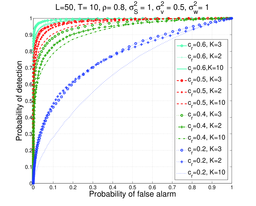
(a) $T=10$

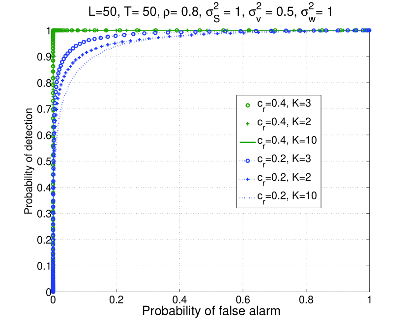
(b) $T=50$

Figure 1: Detection performance with $\Lambda_{C}$ as $c_{r}$ and $K$ vary for given $T$ and $L$, $L=50$ , $\rho=0.8$

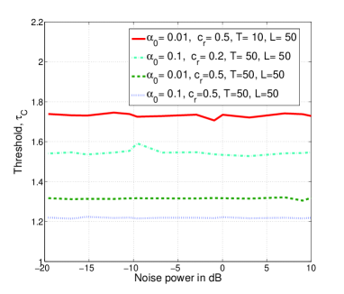
Figure 2: Threshold, to keep $P_{f}\leq\alpha_{0}$, of the covariance based detector with $\Lambda_{C}$ vs $10\log_{10}{\sigma_{\tilde{w}}^{2}}$

Let the desired probability of false alarm be $\alpha_{0}$. In order to find the threshold of the detector with $\Lambda_{C}$, we need to find $\tau_{C}$ so that $Pr(\Lambda_{C}\geq\tau_{C}|\mathcal{H}_{0})\leq\alpha_{0}$, which is analytically difficult. In Fig. 2, we plot $\tau_{C}$ computed numerically as $\sigma_{\tilde{w}}^{2}$ varies keeping $L$, $T$ and $M$ fixed. The noise power along the $x$-axis is taken as $10\log_{10}(\sigma_{\tilde{w}}^{2})$. It can be observed that, the threshold is independent of the noise parameter for given $T$, $L$ and $c_{r}$ which makes the compressive covariance based detector attractive compared to the other non parametric detectors such as the energy detector.

Next, we illustrate the robustness of the proposed detector compared to the energy detector. The decision statistic of the energy detector is given by $\Lambda_{E}=\sum_{n=1}^{T}||\mathbf{y}[n]||^{2}$. Approximating $\Lambda_{E}$ to be Gaussian under $\mathcal{H}_{0}$, the threshold of the energy detector to keep $P_{f}\leq\alpha_{0}$, $\tau_{E}$, can be found as $\tau_{E}=\sigma_{\tilde{w}}^{2}\left(\sqrt{2MT}Q^{-1}(\alpha_{0})+MT\right)$ which is a function of $\sigma_{\tilde{w}}^{2}$ where $Q^{-1}(\cdot)$ denotes the inverse Gaussian $Q$ function. The estimated or the assumed noise power in many practical receivers can be different from the real noise power. Let $\tilde{\sigma}_{\tilde{w}}^{2}$ be the estimated noise power, which can be expressed as $\tilde{\sigma}_{\tilde{w}}^{2}=\beta_{w}\sigma_{\tilde{w}}^{2}$. The noise uncertainty factor is defined as $\beta=\max\{10\log_{10}\beta_{w}\}$ [29]. As in [29], we assume that $\beta_{w}$ is uniformly distributed over $[-\beta,\beta]$. In Fig. 3, $P_{d}$ and $P_{f}$ vs SNR are plotted when detection is performed with $\Lambda_{C}$ and $\Lambda_{E}$ setting the threshold so the $\alpha_{0}=0.1$. To vary SNR, we vary $\sigma_{v}^{2}$ keeping $\sigma_{S}^{2}$ and $\sigma_{w}^{2}$ fixed. With $\Lambda_{C}$, we compute the threshold numerically for given $L$, $c_{r}$, and taking $\sigma_{v}^{2}=0.5$ and $\sigma_{w}^{2}=0.1$ and keep it the same as SNR varies. With $\Lambda_{E}$, we plot $P_{d}$ and $P_{f}$ in the presence of noise variance uncertainty (as $\beta$ varies) as well as when it is assumed that there in no uncertainty.

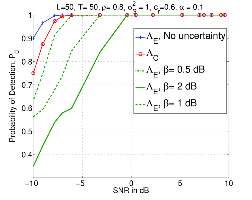
(a) $P_{d}$

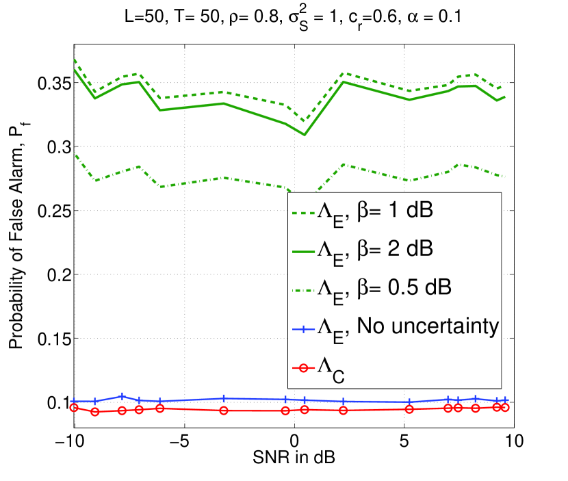
(b) $P_{f}$

Figure 3: Probability of detection and false alarm vs SNR

From Fig. 3, it can be seen that when there is no uncertainty in the estimated noise power, the energy detector has better detection performance than the covariance based detector. However, the performance of the former, in terms of both $P_{d}$ and $P_{f}$, degrades significantly even with small $\beta$. Thus, detection based on $\Lambda_{C}$ appears to be more robust in practical applications than the energy detector.

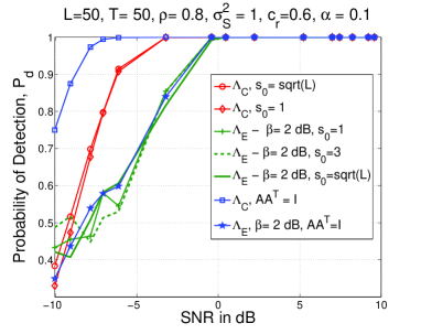
Figure 4: Probability of detection vs SNR with sparse random projections

Next, we investigate the detection performance when the assumption $\mathbf{A}\mathbf{A}^{T}=\mathbf{I}$ is relaxed. In resource constrained sensor networks, the use of sparse random projections for spatial data compression is promising [33, 34, 35] since then not all the sensors need to transmit during a given MAC transmission. To illustrate the detection performance, we select $\mathbf{A}[i,j]$ as

$$\mathbf{A}[i,j]=\sqrt{\frac{s_{0}}{L}}\left\{\begin{array}[]{cccc}1{}&\mathrm{with}~{}\mathrm{prob}~{}\frac{1}{2s_{0}}\\ 0{}&\mathrm{with}~{}\mathrm{prob}~{}1-\frac{1}{s_{0}}\\ -1{}&\mathrm{with}~{}\mathrm{prob}~{}\frac{1}{2s_{0}}\end{array}\right.$$ (16)

with $s_{0}\geq 1$. With this matrix, only $L/s_{0}$ sensors, on an average, need to transmit during a given MAC transmission. When $s_{0}=1$, $\mathbf{A}$ is dense and all the nodes have to transmit. In Fig. 4, we plot $P_{d}$ vs SNR as $s_{0}$ varies with $\Lambda_{C}$ and $\Lambda_{E}$ with $\beta=2dB$. We let $\alpha_{0}=0.1$. We further plot the performance when $\mathbf{A}$ is selected such that $\mathbf{A}\mathbf{A}^{T}=\mathbf{I}$ as considered before so that $\tilde{\bm{\Sigma}}_{x}$ is exactly diagonal under $\mathcal{H}_{0}$. When comparing $\Lambda_{C}$ with $\mathbf{A}$ as in (16) for $s_{0}=1$, to $\Lambda_{C}$ with $\mathbf{A}\mathbf{A}^{T}=\mathbf{I}$, it can be seen from Fig. 4 that the former provides with a degraded performance compared to the latter. This is due to the fact that, with the former, $\tilde{\bm{\Sigma}}_{x}$ is only approximately diagonal under $\mathcal{H}_{0}$ which reduces the distinguishability between the two hypotheses. However, compared to the energy detector with noise uncertainty, $\Lambda_{C}$ with $\mathbf{A}$ as in (16) even with very small $1/s_{0}$ provides much better detection performance. Further, it is seen that the sparsity parameter of $\mathbf{A}$ in (16), $s_{0}$, does not impact on the detection performance significantly. Thus, it is sufficient for only a small number of nodes (e.g., $\sqrt{L}$ on average) to transmit observations to achieve almost the same performance as when all the $L$ nodes transmit with the matrix $\mathbf{A}$ in (16).

V Conclusion

In this paper, we have proposed a nonparametric detection method exploiting CS to detect a random event using spatially correlated data in a sensor network. To transmit a compressed version of spatially correlated data at the fusion center, the MAC model was employed. A test statistic based on the covariance matrix of uncompressed data was considered which was computed based on the limited compressed samples received at the fusion center. Unlike the widely used energy detector, the proposed detector does not need exact estimates of the noise power to set the threshold. Further, the proposed detector is robust to the selection of the sparsity parameter of the random projection matrix when sparse random projections are employed to reduce the communication overhead.

References

- [1] I. Akyildiz, W. Su, Y. Sankarasubramaniam, and E. Cayirci, “Wireless sensor networks: a survey,” Computer Networks, vol. 38, no. 4, 2002.
- [2] D. Puccinelli and M. Haenggi, “Wireless sensor networks: Applications and challenges of ubiquitous sensing,” IEEE Circuits Syst. Mag., vol. 5, no. 3, pp. 19–31, 2005.
- [3] J. Yick, B. Mukherjee, and D. Ghosal, “Wireless sensor network survey,” Computer Networks, vol. 52, no. 12, pp. 2292–2330, 2008.
- [4] L. Mainetti, L. Patrono, and A. Vilei, “Evolution of wireless sensor networks towards the internet of things: A survey,” in 19th International Conference on Software, Telecommunications and Computer Networks (SoftCOM), 2011, pp. 1–6.
- [5] J. A. Stankovic, A. D. Wood, and T. He, “Realistic applications for wireless sensor networks,” Theoretical Aspects of Distributed Computing in Sensor Networks Springer, pp. 853–863, 2011.
- [6] M. F. Othman and K. Shazali, “Wireless sensor network applications: A study in environment monitoring system,” Engineering Procedia, vol. 41, pp. 1204–1210, 2012.
- [7] P. Rawat, K. D. Singh, H. Chaouchi, and J. M. Bonnin, “Wireless sensor networks: a survey on recent developments and potential synergies,” Journal of supercomputing, vol. 68, no. 1, pp. 1–48, 2014.
- [8] B. Rashid and M. H. Rehmani, “Applications of wireless sensor networks for urban areas: A survey,” Journal of Network and Computer Applications, vol. 60, pp. 192–219, 2016.
- [9] M. F. Duarte, M. B. Wakin, D. Baron, S. Sarvotham, and R. G. Baraniuk, “Measurement bounds for sparse signal ensembles via graphical models,” IEEE Trans. Inf. Theory, vol. 59, no. 7, pp. 4280–4289, Jul. 2013.
- [10] J. Haupt, W. U. Bajwa, M. Rabbat, and R. Nowak, “Compressed sensing for networked data,” IEEE Signal Process. Mag., vol. 25, no. 2, pp. 92–101, Mar. 2008.
- [11] J. Meng, H. Li, and Z. Han, “Sparse event detection in wireless sensor networks using compressive sensing,” in 43rd Annual Conf. on Information Sciences and Systems (CISS), Baltimore, MD, Mar. 2009, pp. 181 – 185.
- [12] C. Feng, S. Valaee, and Z. H. Tan, “Multiple target localization using compressive sensing,” in IEEE Global Telecommunications Conference (GLOBECOM), Dec. 2009.
- [13] B. Zhang, X. Cheng, N. Zhang, Y. Cui, Y. Li, and Q. Liang, “Sparse target counting and localization in sensor networks based on compressive sensing,” in INFOCOM, 2011.
- [14] M. F. Duarte, M. A. Davenport, M. B. Wakin, and R. G. Baraniuk, “Sparse signal detection from incoherent projections,” in Proc. Acoust., Speech, Signal Processing (ICASSP), May 2006.
- [15] J. Haupt and R. Nowak, “Compressive sampling for signal detection,” in Proc. Acoust., Speech, Signal Processing (ICASSP), vol. 3, Honolulu, Hawaii, Apr. 2007, pp. III–1509 – III–1512.
- [16] G. Li, H. Zhang, T. Wimalajeewa, and P. K. Varshney, “On the detection of sparse signals with sensor networks based on Subspace Pursuit,” in IEEE Global Conference on Signal and Information Processing (GlobalSIP), Atlanta, GA, Dec. 2014, pp. 438–442.
- [17] B. S. M. R. Rao, S. Chatterjee, and B. Ottersten, “Detection of sparse random signals using compressive measurements,” in Proc. Acoust., Speech, Signal Processing (ICASSP), 2012, pp. 3257–3260.
- [18] J. Cao and Z. Lin, “Bayesian signal detection with compressed measurements,” Information Sciences, pp. 241–253, 2014.
- [19] T. Wimalajeewa and P. K. Varshney, “Sparse signal detection with compressive measurements via partial support set estimation,” IEEE Trans. on Signal and Inf. Process. over Netw., vol. 3, no. 1, Mar. 2017.
- [20] M. A. Davenport, P. T. Boufounos, M. B. Wakin, and R. Baraniuk, “Signal processing with compressive measurements,” IEEE J. Sel. Topics Signal Process., vol. 4, no. 2, pp. 445 – 460, Apr. 2010.
- [21] T. Wimalajeewa, H. Chen, and P. K. Varshney, “Performance analysis of stochastic signal detection with compressive measurements,” in Annual Asilomar Conf. on Signals, Systems and Computers, Nov. 2010, pp. 913–817.
- [22] B. Kailkhura, T. Wimalajeewa, L. Shen, and P. K. Varshney, “Distributed compressive detection with perfect secrecy,” in 2nd Int. Workshop on Compressive Sensing in Cyber-Physical Systems (CSCPS’14), Oct. 2014.
- [23] B. Kailkhura, T. Wimalajeewa, and P. K. Varshney, “On physical layer secrecy of collaborative compressive detection,” in Annual Asilomar Conf. on Signals, Systems and Computers, 2014.
- [24] M. Vuran, O. Akan, and I. Akyildiz, “Spatio-temporal correlation: Theory and applications for wireless sensor networks,” Comput. Networks (Elsevier), vol. 45, no. 3, pp. 245–259, 2004.
- [25] J. Berger, V. de Oliviera, and B. Sanso, “Objective bayesian analysis of spatially correlated data,” J. Am. Statist. Assoc., vol. 96, pp. 1361–1374, 2001.
- [26] D. Romero, D. Ariananda, Z. Tian, and G. Leus, “Compressive covariance sensing: Structure-based compressive sensing beyond sparsity,” IEEE Signal Process. Mag., vol. 33, no. 1, pp. 78–93, Jan. 2016.
- [27] W. Bajwa, J. Haupt, A. Sayeed, and R. Nowak, “Joint source–channel communication for distributed estimation in sensor networks,” IEEE Trans. Inf. Theory, vol. 53, no. 10, pp. 3629–3653, Oct. 2007.
- [28] T. Wimalajeewa and P. K. Varshney, “Compressive sensing based detection with multimodal-dependent data,” Online available,https://arxiv.org/pdf/1701.01352.pdf, 2017.
- [29] Y. Zeng and Y.-C. Liang, “Covariance based signal detections for cognitive radio,” in IEEE Int. Symposium on New Frontiers in Dynamic Spectrum Access Networks, Dublin, Ireland, Apr. 2007, pp. 202–207.
- [30] ——, “Spectrum-sensing algorithms for cognitive radio based on statistical covariances,” IEEE Trans. Veh. Technol., vol. 58, no. 4, pp. 1804–1815, May 2009.
- [31] J. Bioucas-Dias, D. Cohen, , and Y. Eldar, “Covalsa: Covariance estimation from compressive measurements using alternating minimization,” in 2014 Proceedings of the 22nd European Signal Processing Conference (EUSIPCO), Sept. 2014, pp. 999–1003.
- [32] T. Wimalajeewa, Y. C. Eldar, and P. K. Varshney, “Recovery of sparse matrices via matrix sketching,” CoRR, vol. abs/1311.2448, 2013.
- [33] W. Wang, M. Garofalakis, and K. Ramchandran, “Distributed sparse random projections for refinable approximation,” in ISPN, Cambridge, Massachusetts,USA, April 2007, pp. 331–339.
- [34] G. Yang, V. Tan, C. Ho, S. Ting, and Y. Guan, “Wireless compressive sensing for energy harvesting sensor nodes,” IEEE Trans. Signal Process., vol. 61, p. 4491 – 4505, Sept. 2013.
- [35] T. Wimalajeewa and P. K. Varshney, “Wireless compressive sensing over fading channels with distributed sparse random projections,” IEEE Trans. Signal and Inf. Process. over Netw, vol. 1, no. 1, Mar. 2015.