A Fully Quaternion-Valued Capon Beamformer Based on Crossed-Dipole Arrays

Abstract

Quaternion models have been developed for both direction of arrival estimation and beamforming based on crossed-dipole arrays in the past. However, for almost all the models, especially for adaptive beamforming, the desired signal is still complex-valued and one example is the quaternion-Capon beamformer. However, since the complex-valued desired signal only has two components, while there are four components in a quaternion, only two components of the quaternion-valued beamformer output are used and the remaining two are simply removed. This leads to significant redundancy in its implementation. In this work, we consider a quaternion-valued desired signal and develop a full quaternion-valued Capon beamformer, which has a better performance and a much lower complexity and is shown to be more robust against array pointing errors.

Keywords — quaternion model, crossed-dipole, Capon beamformer, vector sensor array.

I Introduction

Electromagnetic (EM) vector sensor arrays can track the direction of arrival (DOA) of impinging signals as well as their polarization. A crossed-dipole sensor array, firstly introduced in [1] for adaptive beamforming, works by processing the received signals with a long polarization vector. Based on such a model, the beamforming problem is studied in detail in terms of output signal-to-interference-plus-noise ratio (SINR) [2]. In [3, 4], further detailed analysis was performed showing that the output SINR is affected by DOA and polarization differences.

Since there are four components for each vector sensor output in a crossed-dipole array, a quaternion model instead of long vectors has been adopted in the past for both adaptive beamforming and direction of arrival (DOA) estimation [5, 6, 7, 8, 9]. In [10], the well-known Capon beamformer was extended to the quaternion domain and a quaternion-valued Capon (Q-Capon) beamformer was proposed with the corresponding optimum solution derived.

However, in most of the beamforming studies, the signal of interest (SOI) is still complex-valued, i.e. with only two components: in-phase (I) and quadrature (Q). Since the output of a quaternion-valued beamformer is also quaternion-valued, only two components of the quaternion are used to recover the SOI, which leads to redundancy in both calculation and data storage. However, with the development of quaternion-valued wireless communications [11, 12, 13], it is very likely that in the future we will have quaternion-valued signals as the SOI, where two traditional complex-valued signals with different polarisations arrive at the array with the same DOA. In such a case, a full quaternion-valued array model is needed to compactly represent the four-component desired signal and also make sure the four components of the quaternion-valued output of the beamformer are fully utilised. In this work, we develop such a model and propose a new quaternion-valued Capon beamformer, where both its input and output are quaternion-valued.

This paper is structured as follows. The full quaternion-valued array model is introduced in Section II and the proposed quaternion-valued Capon beamformer is developed in Section III. Simulation results are presented in IV, and conclusions are drawn in Section V.

II Quaternion model for array processing

A quaternion is constructed by four components [14, 15], with one real part and three imaginary parts, which is defined as $q=q_{a}+iq_{b}+jq_{c}+kq_{d}$, where $i,j,k$ are three different imaginary units and $q_{a},q_{b},q_{c},q_{d}$ are real-valued. The multiplication principle among such units is

$$i^{2}=j^{2}=k^{2}=ijk=-1,$$ (1)

and

$$ij=-ji=k,ki=-ik=j,jk=-ki=i$$ (2)

The conjugate $q^{*}$ of $q$ is $q^{*}=q_{a}-iq_{b}-jq_{c}-kq_{d}$.

A quaternion number can be conveniently denoted as a combination of two complex numbers $q=c_{1}+ic_{2}$, where the complex number $c_{1}=q_{a}+jq_{c}$ and $c_{2}=q_{b}+jq_{d}$. We will use this form later to represent our quaternion-valued signal of interest.

Consider a uniform linear array with $N$ crossed-dipole sensors, as shown in Fig. 1, where the adjacent vector sensor spacing $d$ equals half wavelength, and the two components of each crossed-dipole are parallel to $x-$ and $y-$axes, respectively. A quaternion-valued narrowband signal $s_{0}(t)$ impinges upon the vector sensor array among other $M$ uncorrelated quaternion-valued interfering signals $\{s_{m}(t)\}_{m=1}^{M}$, with background noise $n(t)$. $s_{0}(t)$ can be decomposed into

$$s_{0}(t)=s_{01}(t)+is_{02}(t)\;,$$ (3)

where $s_{01}(t)$ and $s_{02}(t)$ are two complex-valued sub-signals with the same DOA but different polarizations.

Assume that all signals are ellipse-polarized. The parameters, including DOA and polarization of the $m$-th signal are denoted by $(\theta_{m},\phi_{m},\gamma_{m1},\eta_{m1})$ for the first sub-signal and $(\theta_{m},\phi_{m},\gamma_{m2},\eta_{m2})$ for the second sub-signal. Each crossed-dipole sensor receives signals both in the $x$ and $y$ sub-arrays.

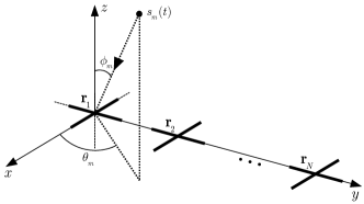
Figure 1: A crossed-dipole linear array with $N$ vector sensors.

For signal $s_{m}(t)$, the corresponding received signals at the $x$ and $y$ sub-arrays are respectively given by [16]:

$$\emph{{x}}(t)=\emph{{a}}_{m1}p_{xm1}s_{m1}(t)+\emph{{a}}_{m2}p_{xm2}s_{m2}(t)$$

$$\emph{{y}}(t)=\emph{{a}}_{m1}p_{ym1}s_{m1}(t)+\emph{{a}}_{m2}p_{ym2}s_{m2}(t)$$ (4)

where $\emph{{x}}(t)$ represents the received part in the x-sub-array, $\emph{{y}}(t)$ represents the part in the y-sub-array, and $(p_{xm1},p_{ym1})$ and $(p_{xm2},p_{ym2})$ are the polarizations of the two complex sub-signals in $x$ and $y$ directions, respectively, which are given by [17],

$$p_{xm1} =-\cos{\gamma_{m1}}$$ (5)

$$p_{ym1} =\cos{\phi_{m}}\sin{\gamma_{m1}}{e}^{j\eta_{m1}}$$

$$p_{xm2} =-\cos{\gamma_{m2}}$$

$$p_{ym2} =\cos{\phi_{m}}\sin{\gamma_{m2}}{e}^{j\eta_{m2}},\quad\text{when}\quad\theta_{m}=\frac{\pi}{2}$$

Note that $\emph{{a}}_{m1}$ and $\emph{{a}}_{m2}$ are the steering vectors for the two sub-signals, which are equal to each other since the two sub-signals share the same DOA $(\theta_{m},\phi_{m})$.

$$\emph{{a}}_{m1}=[1\quad e^{\frac{-j2\pi\sin{\theta_{m}}\sin{\phi_{m}}}{\lambda}},...e^{\frac{-j(N-1)2\pi\sin{\theta_{m}}\sin{\phi_{m}}}{\lambda}}]^{\text{T}}$$

$$\emph{{a}}_{m2}=[1\quad e^{\frac{-j2\pi\sin{\theta_{m}}\sin{\phi_{m}}}{\lambda}},...e^{\frac{-j(N-1)2\pi\sin{\theta_{m}}\sin{\phi_{m}}}{\lambda}}]^{\text{T}}$$ (6)

A quaternion model can be constructed by combining the two parts as below:

$$\emph{{q}}_{m}(t) =\emph{{x}}(t)+i\emph{{y}}(t)$$ (8)

$$=\emph{{a}}_{m1}(p_{xm1}+ip_{ym1})s_{m1}(t)$$

$$+\emph{{a}}_{m2}(p_{xm2}+ip_{ym2})s_{m2}(t)$$

$$=\emph{{b}}_{m1}s_{m1}(t)+\emph{{b}}_{m2}s_{m2}(t)$$

where $\{\emph{{b}}_{m1},\emph{{b}}_{m2}\}\in\mathbb{H}^{N\times 1}$ can be considered as the composite quaternion-valued steering vector. Combining all source signals and the noise together, the result is given by:

$$\emph{{q}}(t)=\sum\limits^{M}_{m=0}(\emph{{b}}_{m1}s_{m1}(t)+\emph{{b}}_{m2}s_{m2}(t))+\emph{{n}}_{q}(t)$$ (9)

where $\emph{{n}}_{q}(t)=\emph{{n}}_{x}(t)+i\emph{{n}}_{y}(t)$ is the quaternion-valued noise vector consisting of the two sub-array noise vectors $\emph{{n}}_{x}(t)$ and $\emph{{n}}_{y}(t)$.

III Full quaternion Capon beamformer

III-A The Full Q-Capon Beamformer

To recover the SOI among interfering signals and noise, the basic idea is to keep a unity response to the SOI at the beamformer output and then reduce the power/variance of the output as much as possible [18, 19]. The key to construct such a Capon beamformer in the quaternion domain is to design an appropriate constraint to make sure the quaternion-valued SOI can pass through the beamformer with the desired unity response.

Again note that the quaternion-valued SOI can be expressed as a combination of two complex sub-signals. To construct such a constraint, one choice is to make sure the first complex sub-signal of the SOI pass through the beamformer and appear in the real and $j$ components of the beamformer output, while the second complex sub-signal appear in the $i$ and $k$ components of the beamformer output. Then, with a quaternion-valued weight vector w, the constraint can be formulated as

$$\emph{{w}}^{\text{H}}\emph{{C}}=\emph{{f}}$$ (10)

where $\{\}^{\text{H}}$ is the Hermitian transpose (combination of the quaternion-valued conjugate and transpose operation), $\emph{{C}}=[\emph{{b}}_{01}\quad\emph{{b}}_{02}]$, and $\emph{{f}}=[1\quad i]$.

With this constraint, the beamformer output $z(t)$ is given by

$$z(t) =\emph{{w}}^{\text{H}}\emph{{q}}(t)$$ (11)

$$=\underbrace{s_{01}(t)+is_{02}(t)}_{s_{0}(t)}+\emph{{w}}^{\text{H}}\emph{{n}}_{q}(t)$$

$$\quad+\sum\limits^{M}_{m=1}\emph{{w}}^{\text{H}}[\emph{{b}}_{m1}s_{m1}(t)+\emph{{b}}_{m2}s_{m2}(t)]$$

Clearly, the quaternion-valued SOI has been preserved at the output with the desired unity response.

Now, the full-quaternion Capon (full Q-Capon) beamformer can be formulated as

$$\min \emph{{w}}^{\text{H}}\emph{{R}}\emph{{w}}\text{ subject to }\emph{{w}}^{\text{H}}\emph{{C}}=\emph{{f}}$$ (12)

where

$$\emph{{R}}=E\{\emph{{q}}(t)\emph{{q}}^{\text{H}}(t)\}\;.$$ (13)

Applying the Lagrange multiplier method, we have

$$l(\emph{{w}},\boldsymbol{\lambda})=\emph{{w}}^{\text{H}}\emph{{R}}\emph{{w}}+(\emph{{w}}^{\text{H}}\emph{{C}}-\emph{{f}})\boldsymbol{\lambda}^{\text{H}}+\boldsymbol{\lambda}(\emph{{C}}^{\text{H}}\emph{{w}}-\emph{{f}}^{\text{H}})$$ (14)

where $\boldsymbol{\lambda}$ is a quaternion-valued vector.

The minimum can be obtained by setting the gradient of (14) with respect to $\emph{{w}}^{*}$ equal to a zero vector [20]. It is given by

$$\nabla_{\emph{{w}}^{*}}l(\emph{{w}},\boldsymbol{\lambda})=\frac{1}{2}\emph{{R}}\emph{{w}}+\frac{1}{2}\emph{{C}}\boldsymbol{\lambda}^{\text{H}}=\emph{{0}}$$ (15)

Considering all the constraints above, we obtain the optimum weight vector $\emph{{w}}_{opt}$ as follows

$$\emph{{w}}_{opt}=\emph{{R}}^{-1}\emph{{C}}(\emph{{C}}^{\text{H}}\emph{{R}}^{-1}\emph{{C}})^{-1}\emph{{f}}^{\text{H}}\;.$$ (16)

A detailed derivation for the quaternion-valued optimum weight vector can be found at the Appendix.

In the next subsection, we give a brief analysis to show that by this optimum weight vector, the interference part at the beamformer output $z(t)$ in (11) has been suppressed effectively.

III-B Interference Suppression

Expanding the covariance matrix, we have

$$\emph{{R}}=E\{\emph{{q}}(t)\emph{{q}}^{\text{H}}(t)\}=\emph{{R}}_{i+n}+\sigma^{2}_{1}\emph{{b}}_{01}\emph{{b}}_{01}^{H}+\sigma^{2}_{2}\emph{{b}}_{02}\emph{{b}}_{02}^{\text{H}}$$ (17)

where $\sigma^{2}_{1},\sigma^{2}_{2}$ are the power of the two sub-signals of SOI and $\emph{{R}}_{i+n}$ denotes the covariance matrix of interferences plus noise. Using the Sherman-Morrison formula, we then have

$$\emph{{w}}_{opt}=\emph{{R}}_{i+n}^{-1}\emph{{C}}\boldsymbol{\beta}$$ (18)

where $\boldsymbol{\beta}=(\emph{{C}}^{\text{H}}\emph{{R}}_{i+n}\emph{{C}})^{-1}\emph{{f}}^{\text{H}}\in\mathbb{H}^{2\times 1}$ is a quaternion vector.

Applying left eigendecomposition for quaternion matrix [21, 22, 23],

$$\emph{{R}}_{i+n}=\sum\limits^{N}_{n=1}\alpha_{n}\emph{{u}}_{n}\emph{{u}}_{n}^{\text{H}}$$ (19)

with $\alpha_{1}\geq\text{...}\geq\alpha_{M-2}\textgreater{\alpha_{M-1}}=\text{...}=\alpha_{N}=2\sigma^{2}_{0}\in\mathbb{R}$, where $2\sigma^{2}_{0}$ denotes the noise power.

With sufficiently high interference to noise ratio (INR), the inverse of $\emph{{R}}_{i+n}$ can be approximated by

$$\emph{{R}}_{i+n}^{-1}\approx\sum\limits^{N}_{n=M+1}\frac{1}{2\sigma^{2}_{0}}\emph{{u}}_{n}\emph{{u}}_{n}^{\text{H}}$$ (20)

Then, we have

$$\emph{{w}}_{opt} =\sum\limits^{N}_{n=M+1}\frac{1}{2\sigma^{2}_{0}}\emph{{u}}_{n}\emph{{u}}_{n}^{\text{H}}\emph{{C}}\boldsymbol{\beta}=\sum\limits^{N}_{n=M+1}\emph{{u}}_{n}\rho_{n}$$ (21)

where $\rho_{n}$ is a quaternion-valued constant. Clearly, $\emph{{w}}_{opt}$ is the right linear combination of $\{u_{M+1},u_{M+2},\text{...},u_{N}\}$, and $\emph{{w}}\in\text{$span_{R}$}\{u_{M+1},u_{M+2},\text{...},u_{N}\}$.

For those $M$ interfering signals, their quaternion steering vectors belong to the space right-spanned by the related $M$ eigenvectors, i.e. $\emph{{b}}_{m1},\emph{{b}}_{m2}\in\text{$span_{R}$}\{u_{1},u_{2},\text{...},u_{M}\}$. As a result,

$$\emph{{w}}_{opt}^{\text{H}}\emph{{b}}_{m1}\approx 0,\emph{{w}}_{opt}^{\text{H}}\emph{{b}}_{m2}\approx 0,m=1,4,\text{...},M$$ (22)

which shows that the beamformer has eliminated the interferences effectively.

III-C Complexity Analysis

In this section, we make a comparison of the computation complexity between the Q-Capon beamformer in [10] and our proposed full Q-Capon beamformer. To deal with a quaternion-valued signal, the Q-Capon beamformer has to process the two complex sub-signals separately to recover the desired signal completely, which means we need to apply the beamformer twice for a quaternion-valued SOI. However, for the full Q-Capon beamformer, the SOI is recovered directly by applying the beamformer once.

For the Q-Capon beamformer, the weight vector is calculated by $\textbf{w}=\emph{{R}}^{-1}\emph{{a}}_{0}(\emph{{a}}_{0}^{\text{H}}\emph{{R}}^{-1}\emph{{a}}_{0})^{-1}$, where $\textbf{a}_{0}$ is the steering vector for the complex-valued SOI. As an example, we use Gaussian elimination to calculate the matrix inversion $\emph{{R}}^{-1}$ and $\frac{1}{3}(N^{3}-N)$ quaternion-valued multiplications are needed, equivalent to $\frac{16}{3}(N^{3}-N)$ real-valued multiplications. Additionally, $\emph{{R}}^{-1}\emph{{a}}_{0}$ requires $16N^{2}$ real-valued multiplications, while $16(N^{2}+N)$ real multiplications are needed for $(\emph{{a}}_{0}^{\text{H}}\emph{{R}}^{-1}\emph{{a}}_{0})^{-1}$. In total, $\frac{16}{3}N^{3}+32N^{2}+\frac{80}{3}N$ real multiplications are needed. When processing a quaternion-valued signal, this number will be doubled and the total number of real multiplications becomes $\frac{32}{3}N^{3}+64N^{2}+\frac{160}{3}N$.

For the proposed full Q-Capon beamformer, in addition to calculating $\emph{{R}}^{-1}$, $32N^{2}$ real multiplications are required to calculate $\emph{{R}}^{-1}\emph{{C}}$ and $32M^{2}+32M+96$ real multiplications for $(\emph{{C}}^{\text{H}}\emph{{R}}^{-1}\emph{{C}}_{0})^{-1}\emph{{f}}$. In total, the number of real-valued multiplications is $\frac{16}{3}M^{3}+64M^{2}+\frac{272}{3}M+96$, which is roughly half of that of the Q-Capon beamformer.

IV Simulations Results

In our simulations, we consider $10$ pairs of cross-dipoles with half wave-length spacing. All signals are assumed to arrive from the same plane of $\theta=90\degree$ and all interferences have the same polarization parameter $\gamma=60\degree$. For the SOI, the two sub-signals are set to (90°, 1.5°, 90°, 45°) and (90°, 1.5°, 0°, 0°), with inferences coming from (90°, 30°, 60°, -80°), (90°, -70°, 60°, 30°), (90°, -20°, 60°, 70°), (90°, 50°, 60°, -50°), respectively. The background noise is zero-mean quaternion-valued Gaussian. The power of SOI and all interfering signals are set equal and SNR (INR) is 20dB.

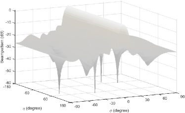
Figure 2: The resultant beam pattern with $\theta=90\degree$ and $\gamma=60\degree$.

Fig. 2 shows the resultant 3-D beam pattern by the proposed beamformer, where the interfering signals from ($\phi,\eta$)=(30°, -80°), (-70°, 30°), (-20°, 70°) and (50°, -50°) have all been effectively suppressed.

In the following, the output SINR performance of the two Capon beamformers (full Q-Capon and Q-Capon) is studied with the DOA and polarization (90°, 1.5°, 90°, 45°) and (90°, 1.5°, 0°, 0°) for SOI and (90°, 30°, 60°, -80°), (90°,- 70°, 60°, 30°), (90°, -20°, 60°, 70°), (90°, 50°, 60°, -50°) for interferences. Again, we have set SNR=INR=20dB. All results are obtained by averaging 1000 Monte-Carlo trials.

Fig. 3 shows the output SINR performance versus SNR with $100$ snapshots, where the solid-line is for the optimal beamformer with infinite number of snapshots. For most of the input SNR range, in particular the lower range, the proposed full Q-Capon beamformer has a better performance than the Q-Capon beamformer. For very high input SNR values, these two beamformers have a very similar performance.

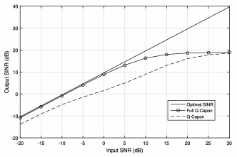
Figure 3: Output SINR versus input SNR (snapshots number 100).

Next, we investigate their performance in the presence of DOA and polarization errors. The output SINR with respect to the number of snapshots is shown in Fig. 4 in the presence of $1\degree$ error for the SOI, where the real DOA and polarization parameters are (91°,2.5°,91°,46°) and (91°,2.5°,1°,1°). It can be seen that the full Q-Capon beamformer has achieved a much higher output SINR than the Q-Capon beamformer, and this gap increases with the increase of snapshot number. Fig. 5 shows a similar trend in the presence of a $5\degree$ error. Overall, we can see that the proposed full Q-Capon beamformer is more robust against array pointing errors.

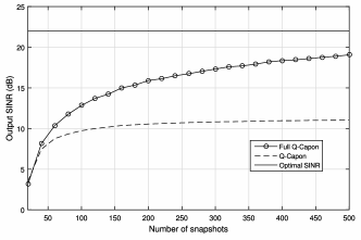
Figure 4: Output SINR versus snapshot number with SNR=SIR=15dB and 1°error.

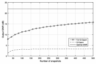
Figure 5: Output SINR versus snapshot number with SNR=SIR=15dB and 5°error.

V Conclusions

In this paper, a full quaternion model has been developed for adaptive beamforming based on crossed-dipole arrays, with a new full quaternion Capon beamformer proposed. Different from previous studies in quaternion-valued adaptive beamforming, we have considered a quaternion-valued desired signal, given the recent development in quaternion-valued wireless communications research. The proposed beamformer has a better performance and a much lower computational complexity than a previously proposed Q-Capon beamformer and is also shown to be more robust against array pointing errors, as demonstrated by computer simulations.

The gradient of a quaternion vector $\textbf{u}=\emph{{w}}^{\text{H}}\emph{{C}}\boldsymbol{\lambda}^{\text{H}}$ with respect to $\emph{{w}}^{*}$ can be calculated as below:

$$\nabla_{\emph{{w}}^{*}}{\textbf{u}} =[\nabla_{\emph{{w}}_{1}^{*}}\textbf{u}\quad\nabla{\emph{{w}}_{2}^{*}}\textbf{u}\quad\text{...}\nabla_{\emph{{w}}_{n}^{*}}\textbf{u}]^{T}$$ (23)

where $w_{n}$, $n=1,2,\cdots,N$ is the $n$-th quaternion-valued coefficient of the beamformer. Then,

$$\nabla_{\emph{{w}}_{1}^{*}}{\textbf{u}} =\frac{1}{4}(\nabla_{\emph{{w}}_{1a}}{\textbf{u}}+\nabla_{\emph{{w}}_{1b}}{\textbf{u}}i+\nabla_{\emph{{w}}_{1c}}\textbf{u}j+\nabla_{\emph{{w}}_{1d}}\textbf{u}k)$$ (24)

where

$$\emph{{w}}_{1}^{*}=\emph{{w}}_{1a}-\emph{{w}}_{1b}i-\emph{{w}}_{1c}j-\emph{{w}}_{1d}k$$ (25)

Since $\emph{{w}}_{1a}$ is real-valued, with the chain rule [20], we have

$$\nabla_{\emph{{w}}_{1a}}\textbf{u} =\nabla_{\emph{{w}}_{1a}}({\emph{{w}}^{\text{H}}})\emph{{C}}\boldsymbol{\lambda}^{\text{H}}+\emph{{w}}^{\text{H}}\nabla_{\emph{{w}}_{1a}}({\emph{{C}}\boldsymbol{\lambda}^{\text{H}}})$$ (26)

$$=[1\quad 0\quad 0\quad\text{...}\quad 0]\emph{{C}}\boldsymbol{\lambda}^{\text{H}}$$

Similarly,

$$\nabla_{\emph{{w}}_{1b}}\textbf{u} =[-i\quad 0\quad 0\quad\text{...}\quad 0]\emph{{C}}\boldsymbol{\lambda}^{\text{H}}$$

$$\nabla_{\emph{{w}}_{1c}}\textbf{u} =[-j\quad 0\quad 0\quad\text{...}\quad 0]\emph{{C}}\boldsymbol{\lambda}^{\text{H}}$$

$$\nabla_{\emph{{w}}_{1d}}\textbf{u} =[-k\quad 0\quad 0\quad\text{...}\quad 0]\emph{{C}}\boldsymbol{\lambda}^{\text{H}}$$

Hence,

$$\nabla_{\emph{{w}}_{1}^{*}}\textbf{u} =\frac{1}{4}(4{\text{Real}}(\emph{{C}}\boldsymbol{\lambda}^{\text{H}})_{1})={\text{Real}}(\emph{{C}}\boldsymbol{\lambda}^{\text{H}})_{1}\;,$$ (27)

where the subscript $\{\}_{1}$ in the last item means taking the first entry of the vector.

Finally,

$$\nabla_{\emph{{w}}^{*}}\textbf{u}={\text{Real}}(\emph{{C}}\boldsymbol{\lambda}^{\text{H}})$$ (28)

The gradient of the quaternion vector $\textbf{v}=\boldsymbol{\lambda}\emph{{C}}^{\text{H}}\emph{{w}}$ with respect to $\emph{{w}}^{*}$ can be calculated in the same way:

$$\nabla_{\emph{{w}}_{1a}}\textbf{v} =\boldsymbol{\lambda}\emph{{C}}^{\text{H}}\nabla_{\emph{{w}}_{1a}}\emph{{w}}+\nabla_{\emph{{w}}_{1a}}(\boldsymbol{\lambda}\emph{{C}}^{\text{H}})\emph{{w}}$$ (29)

$$=\boldsymbol{\lambda}\emph{{C}}^{\text{H}}[1\quad 0\quad 0\quad\text{...}\quad 0]^{\text{T}}$$

Similarly,

$$\nabla_{\emph{{w}}_{1b}}\textbf{v} =\boldsymbol{\lambda}\emph{{C}}^{\text{H}}[i\quad 0\quad 0\quad\text{...}\quad 0]^{\text{T}}$$ (30)

$$\nabla_{\emph{{w}}_{1c}}\textbf{v} =\boldsymbol{\lambda}\emph{{C}}^{\text{H}}[j\quad 0\quad 0\quad\text{...}\quad 0]^{\text{T}}$$

$$\nabla_{\emph{{w}}_{1d}}\textbf{v} =\boldsymbol{\lambda}\emph{{C}}^{\text{H}}[k\quad 0\quad 0\quad\text{...}\quad 0]^{\text{T}}$$

Thus, the gradient can be expressed as

$$\nabla_{\emph{{w}}_{1}^{*}}\textbf{v} =-\frac{1}{2}(\emph{{C}}\boldsymbol{\lambda}^{\text{H}})_{1}^{*}$$ (31)

Finally,

$$\nabla_{\emph{{w}}^{*}}\textbf{v}=-\frac{1}{2}(\emph{{C}}\boldsymbol{\lambda}^{\text{H}})^{*}$$ (32)

The gradient of $c_{\textbf{w}}={\emph{{w}}^{\text{H}}\emph{{R}}\emph{{w}}}$ can be calculated as follows.

$$\nabla_{\emph{{w}}^{*}}c_{\textbf{w}}=[\nabla_{\emph{{w}}_{1}^{*}}c_{\textbf{w}}\quad\nabla_{\emph{{w}}_{2}^{*}}c_{\textbf{w}}\quad\text{...}\quad\nabla_{\emph{{w}}_{n}^{*}}c_{\textbf{w}}]^{\text{T}}$$ (33)

$$\nabla_{\emph{{w}}_{1}^{*}}c_{\textbf{w}}=\frac{1}{4}(\nabla_{\emph{{w}}_{1a}}c_{\textbf{w}}+\nabla_{\emph{{w}}_{1b}}c_{\textbf{w}}i+\nabla_{\emph{{w}}_{1c}}c_{\textbf{w}}j+\nabla_{\emph{{w}}_{1d}}c_{\textbf{w}}k)$$ (34)

Now we calculate the gradient of $c_{\textbf{w}}$ with respect to the four components of $\emph{{w}}_{1}$.

$$\nabla_{\emph{{w}}_{1a}}c_{\textbf{w}} =\nabla_{\emph{{w}}_{1a}}({\emph{{w}}^{\text{H}}\emph{{R}}})\emph{{w}}+\emph{{w}}^{\text{H}}\emph{{R}}\nabla_{\emph{{w}}_{1a}}{\emph{{w}}}$$ (35)

$$=[1\quad 0\quad 0\quad\text{...}\quad 0]\emph{{R}}\emph{{w}}$$

$$\quad+\emph{{w}}^{\text{H}}\emph{{R}}[1\quad 0\quad 0\quad\text{...}\quad 0]^{\text{T}}$$

The other three components are,

$$\nabla_{\emph{{w}}_{1b}}c_{\textbf{w}} =[-i\quad 0\quad 0\quad\text{...}\quad 0]\emph{{R}}\emph{{w}}$$

$$\quad+\emph{{w}}^{\text{H}}\emph{{R}}[i\quad 0\quad 0\quad\text{...}\quad 0]^{\text{T}}$$

$$\nabla_{\emph{{w}}_{1c}}c_{\textbf{w}} =[-j\quad 0\quad 0\quad\text{...}\quad 0]\emph{{R}}\emph{{w}}$$

$$\quad+\emph{{w}}^{\text{H}}\emph{{R}}[j\quad 0\quad 0\quad\text{...}\quad 0]^{\text{T}}$$

$$\nabla_{\emph{{w}}_{1d}}c_{\textbf{w}} =[-k\quad 0\quad 0\quad\text{...}\quad 0]\emph{{R}}\emph{{w}}$$

$$\quad+\emph{{w}}^{\text{H}}\emph{{R}}[k\quad 0\quad 0\quad\text{...}\quad 0]^{\text{T}}$$

Hence,

$$\nabla_{\emph{{w}}_{1}^{*}}c_{\textbf{w}} ={\text{Real}}(\emph{{R}}\emph{{w}})_{1}-\frac{1}{2}(\emph{{R}}\emph{{w}})_{1}^{*}=\frac{1}{2}(\emph{{R}}\emph{{w}})_{1}$$ (36)

Finally,

$$\nabla_{\emph{{w}}^{*}}c_{\textbf{w}}=\frac{1}{2}\emph{{R}}\emph{{w}}$$ (37)

Combining (28), (32) and (37), with (14), we have

$$\nabla_{\emph{{w}}^{*}}l(\emph{{w}},\boldsymbol{\lambda})=\frac{1}{2}(\emph{{R}}\emph{{w}}+\emph{{C}}\boldsymbol{\lambda}^{\text{H}})={\textbf{0}}$$ (38)

Further,

$$\emph{{w}}=-2\emph{{R}}^{-1}\emph{{C}}\boldsymbol{\lambda}^{\text{H}}$$ (39)

Subsituting (39) into (10),

$$\boldsymbol{\lambda}=-\frac{1}{2}\emph{{f}}(\emph{{C}}^{\text{H}}\emph{{R}}^{-1}\emph{{C}})^{-1}$$ (40)

Finally,

$$\emph{{w}}=\emph{{R}}^{-1}\emph{{C}}(\emph{{C}}^{\text{H}}\emph{{R}}^{-1}\emph{{C}})^{-1}\emph{{f}}^{\text{H}}$$ (41)

References

• [1] R. Compton Jr, “On the performance of a polarization sensitive adaptive array,” IEEE Transactions on Antennas and Propagation, vol. 29, no. 5, pp. 718–725, September 1981.
• [2] A. Nehorai, K. C. Ho, and B. T. G. Tan, “Minimum-noise-variance beamformer with an electromagnetic vector sensor,” IEEE Transactions on Signal Processing, vol. 47, no. 3, pp. 601–618, March 1999.
• [3] L. C. Godara, “Application of antenna arrays to mobile communications. ii. beam-forming and direction-of-arrival considerations,” Proceedings of the IEEE, vol. 85, no. 8, pp. 1195–1245, August 1997.
• [4] Y. G. Xu, T. Liu, and Z. W. Liu, “Output SINR of MV beamformer with one EM vector sensor of and magnetic noise power,” in Proc. of International Conference on Signal Processing, September 2004, pp. 419–422.
• [5] S. Miron, N. Le Bihan, and J. I. Mars, “High resolution vector-sensor array processing using quaternions,” in Proc. of IEEE Workshop on Statistical Signal Processing, July 2005, pp. 918–923.
• [6] ——, “Quaternion-music for vector-sensor array processing,” IEEE Transactions on Signal Processing, vol. 54, no. 4, pp. 1218–1229, April 2006.
• [7] X. Gong, Y. Xu, and Z. Liu, “Quaternion ESPRIT for direction finding with a polarization sentive array,” in Proc. of International Conference on Signal Processing, October 2008, pp. 378–381.
• [8] J. W. Tao and W. X. Chang, “A novel combined beamformer based on hypercomplex processes,” IEEE Transactions on Aerospace and Electronic Systems, vol. 49, no. 2, pp. 1276–1289, 2013.
• [9] X. R. Zhang, W. Liu, Y. G. Xu, and Z. W. Liu, “Quaternion-valued robust adaptive beamformer for electromagnetic vector-sensor arrays with worst-case constraint,” Signal Processing, vol. 104, pp. 274–283, November 2014.
• [10] X. Gou, Y. Xu, Z. Liu, and X. Gong, “Quaternion-capon beamformer using crossed-dipole arrays,” in Proc. of IEEE International Symposium on Microwave, Antenna, Propagation, and EMC Technologies for Wireless Communications (MAPE), November 2011, pp. 34–37.
• [11] O. M. Isaeva and V. A. Sarytchev, “Quaternion presentations polarization state,” in Proc. 2nd IEEE Topical Symposium of Combined Optical-Microwave Earth and Atmosphere Sensing, Atlanta, US, April 1995, pp. 195–196.
• [12] B. J. Wysocki and T. A. Wysocki, “On an orthogonal space-time-polarization block code,” Journal of Communications, vol. 4, no. 1, pp. 20–25, February 2009.
• [13] W. Liu, “Antenna array signal processing for a quaternion-valued wireless communication system,” in Proc. the Benjamin Franklin Symposium on Microwave and Antenna Sub-systems (BenMAS), Philadelphia, US, September 2014.
• [14] W. R. Hamilton, Elements of Quaternions.   Longmans, Green, & co., 1866.
• [15] I. Kantor, A. S. Solodovnikov, and A. Shenitzer, Hypercomplex Numbers: an Elementary Introduction to Algebras.   New York: Springer Verlag, 1989.
• [16] X. Zhang, W. Liu, Y. Xu, and Z. Liu, “quaternion-valued robust adaptive beamformer for electromagnetic vector-sensor arrays with worst-case constraint,” Signal Processing, vol. 104, pp. 274–283, November 2014.
• [17] M. Hawes and W. Liu, “Design of fixed beamformers based on vector-sensor arrays,” International Journal of Antennas and Propagation, vol. 2015, April 2015.
• [18] J. Capon, “High-resolution frequency-wavenumber spectrum analysis,” Proceedings of the IEEE, vol. 57, no. 8, pp. 1408–1418, August 1969.
• [19] O. L. Frost, III, “An algorithm for linearly constrained adaptive array processing,” Proceedings of the IEEE, vol. 60, no. 8, pp. 926–935, August 1972.
• [20] M. D. Jiang, Y. Li, and W. Liu, “Properties of a general quaternion-valued gradient operator and its application to signal processing,” Frontiers of Information Technology & Electronic Engineering, vol. 17, pp. 83–95, February 2016.
• [21] F. Zhang, “Quaternions and matrices of quaternions,” Linear algebra and its applications, vol. 251, pp. 21–57, January 1997.
• [22] L. Huang and W. So, “On left eigenvalues of a quaternionic matrix,” Linear algebra and its applications, vol. 323, no. 1, pp. 105–116, January 2001.
• [23] N. Le Bihan and J. Mars, “Singular value decomposition of quaternion matrices: a new tool for vector-sensor signal processing,” Signal processing, vol. 84, no. 7, pp. 1177–1199, July 2004.