Detection of Extraplanar Diffuse Ionized Gas in M83^∗

Abstract

We present the first kinematic study of extraplanar diffuse ionized gas (eDIG) in the nearby, face-on disk galaxy M83 using optical emission-line spectroscopy from the Robert Stobie Spectrograph on the Southern African Large Telescope. We use a Markov Chain Monte Carlo method to decompose the [NII]$\lambda\lambda$6548, 6583, H$\alpha$, and [SII]$\lambda\lambda$6717, 6731 emission lines into HII region and diffuse ionized gas emission. Extraplanar, diffuse gas is distinguished by its emission-line ratios ([NII]$\lambda$6583/H$\alpha\mathrel{\hbox{\hbox to0.0pt{\hbox{\lower 4.0pt\hbox{$\sim$}}\hss}\hbox{$>$}}}1.0$) and its rotational velocity lag with respect to the disk ($\Delta v=-24$  km s^-1in projection). With interesting implications for isotropy, the velocity dispersion of the diffuse gas, $\sigma=96$  km s^-1, is a factor of a few higher in M83 than in the Milky Way and nearby, edge-on disk galaxies. The turbulent pressure gradient is sufficient to support the eDIG layer in dynamical equilibrium at an electron scale height of $h_{z}=1$ kpc. However, this dynamical equilibrium model must be finely tuned to reproduce the rotational velocity lag. There is evidence of local bulk flows near star-forming regions in the disk, suggesting that the dynamical state of the gas may be intermediate between a dynamical equilibrium and a galactic fountain flow. As one of the first efforts to study eDIG kinematics in a face-on galaxy, this study demonstrates the feasibility of characterizing the radial distribution, bulk velocities, and vertical velocity dispersions in low-inclination systems.

1. Introduction

The formation and evolution of multi-phase, gaseous galactic halos is affected by star-formation feedback in galactic disks, determining the pressure in the midplane, the enrichment of the intergalactic medium, and the distribution of baryons in the universe. To understand the cycling of mass and energy between the disk and the halo, we must understand the nature of the disk-halo interface, including its structure, energetics, and dynamics.

The dynamical state of the warm ionized phase of this interface, known as the Reynolds Layer in the Milky Way, is not well understood. These extraplanar diffuse ionized gas (eDIG) layers are common in star-forming disk galaxies (Lehnert & Heckman, 1995; Rossa & Dettmar, 2003), but their observed exponential electron scale heights tend to greatly exceed their thermal scale heights (e.g., Rand, 1997; Haffner et al., 1999; Collins & Rand, 2001). Thus, it is not known whether these layers are in dynamical equilibrium, or are evidence of a non-equilibrium state such as a galactic fountain, a galactic wind, or an accretion flow.

Studies of the dynamical state of extraplanar gas layers have largely focused on nearby edge-on disk galaxies (e.g., Collins et al., 2002; Barnabè et al., 2006; Fraternali & Binney, 2006; Boettcher et al., 2016, hereafter B16). In these systems, the gas density, rotational velocity, and horizontal velocity dispersion can be determined as functions of height above the disk, and the contributions of thermal and non-thermal pressure gradients to the vertical structure and support can be quantified. The observed exponential electron scale heights of eDIG layers are on the order of $h_{z}=1$ kpc, and may exceed this value by a factor of a few (e.g., Rand, 1997; Haffner et al., 1999; Collins & Rand, 2001). The thermal velocity dispersion of a $T\sim 10^{4}$ K gas is $\sigma\sim 10$  km s^-1, corresponding to a thermal scale height of only $h_{z}=100-200$ pc. The turbulent velocity dispersions - measured parallel to the disk - tend to be a few tens of  km s^-1, increasing the scale height to only a few hundred parsecs (Heald et al. 2006b, a; B16). Even accounting for thermal, turbulent, magnetic field, and cosmic ray pressure gradients, the eDIG layer in NGC 891 cannot be supported at $h_{z}=1$ kpc at $R\leq 8$ kpc (B16).

Studies of eDIG layers in low-inclination disk galaxies provide a complementary - and largely unexploited - perspective on studies of high-inclination systems. In a face-on galaxy, the vertical velocity dispersion can be directly measured, and one does not have to rely on the assumption that the velocity dispersion is isotropic. Additionally, any vertical bulk flows can be detected, and the radial distribution of the gas can be determined, with particular attention to the relationship between eDIG properties and underlying disk features. Fraternali et al. (2004) demonstrated the feasibility of detecting lagging, extraplanar emission in the moderately-inclined galaxy NGC 2403 using optical emission-line spectroscopy. However, this approach has not been widely applied.

By studying a sample of galaxies with a range of inclination angles, the complete kinematics of eDIG layers can be pieced together. From such a sample, we can address the three-dimensional density distribution, velocity profile, and velocity dispersion, and assess any dependence on the underlying disk properties. Beyond the dynamical state of the eDIG layer itself, these studies will shed light on the isotropy of the velocity dispersion, turbulent and bulk motions relevant to magnetic dynamos, and the relationship between the extraplanar cold, warm, and hot phases.

Here, we perform a study of the eDIG layer in the well-studied disk galaxy M83 (NGC 5236) using optical emission-line spectroscopy from the Robert Stobie Spectrograph on the Southern African Large Telescope. M83 is a nearby ($D=4.8$ Mpc; $1"=23.3$ pc; Karachentsev et al. 2007), face-on ($i=24^{\circ}$; Park et al. 2001) spiral galaxy with an SAB(s)c classification in the Third Reference Catalog of Bright Galaxies (de Vaucouleurs et al., 1991). It has a modest star-formation rate of $SFR=3.2$ M_⊙ yr^-1 (Jarrett et al., 2013), with much of its star formation concentrated in nuclear star clusters. The mass, morphology, and star-formation rate of this system are similar to that of the well-studied, edge-on galaxy NGC 891; thus, a comparison of the eDIG properties in these galaxies is of particular interest.

Observations of M83 from the radio to the X-ray regimes have revealed a complex, multi-phase gaseous halo. M83 has an extended HI disk that is detected to $R>50$ kpc, with warped and filamentary structure suggestive of interactions with a companion (Miller et al. 2009, Heald et al. 2016). In the inner disk, Miller et al. (2009) detect extraplanar HI with a rotational velocity lag of 40 - 50  km s^-1in projection and a line-of-sight velocity dispersion of $\sigma=10-15$  km s^-1. $\sigma$ may be underestimated if the wings of the thick disk emission are compromised by the removal of the thin disk. Within $R=8$ kpc, there are $5.6\times 10^{7}\mbox{\,$M_{\odot}$}$ of extraplanar HI, with a comparable amount of mass in high-velocity, neutral clouds. Miller et al. (2009) interpret these observations as indicative of a galactic fountain coupled with tidal interactions.

Chandra X-ray Observatory observations reveal diffuse, soft X-ray emission that traces the nucleus and spiral arms of M83 (Soria & Wu, 2002, 2003; Long et al., 2014). In the starburst nucleus, the diffuse, hot gas has a temperature of $T\sim 7\times 10^{6}$ K, a redshifted velocity of $\sim 7000$  km s^-1, and abundances consistent with enrichment by Type-II supernovae and stellar winds from Wolf-Rayet stars (Soria & Wu, 2002). This is suggestive of diffuse, hot gas near areas of star-formation activity, and perhaps of a star-formation-driven nuclear outflow. The role of hot halos in the vertical support of the warm phase and the interaction between galactic outflows and eDIG layers remain open questions.

The layout of this paper is as follows. In §2, we discuss the data acquisition, data reduction, and flux calibration. We detail the use of a Markov Chain Monte Carlo method to model the emission-line spectra as superpositions of HII region and diffuse emission in §3. In §4.1, we identify the diffuse emission from its emission-line ratios. In §4.2, we discuss the kinematics of the diffuse gas, including the line-of-sight velocity and velocity dispersion, and we kinematically identify the eDIG layer. We consider the proximity of our eDIG detections to star-forming regions in §4.3, and we estimate the total mass of the layer in §5. We test a dynamical equilibrium model of the eDIG layer in §6. In §7, we compare our results to observations of M83, the Milky Way, and nearby edge-on disk galaxies in the literature, and discuss the merits of both equilibrium and non-equilibrium models. We summarize and conclude in §8.

2. Observations

We obtained observations on 2016 April 04 - 15 using the Robert Stobie Spectrograph (Burgh et al., 2003; Kobulnicky et al., 2003) on the Southern African Large Telescope (SALT; Buckley et al. 2006). The $8^{\prime}$ longslits are centered on the nucleus at two position angles, and, where possible, lie along dust lanes, between spiral arms, and away from HII regions to favor faint extraplanar emission. We obtained observations at low and moderate spectral resolution. The former use a $1.5"$ slit and the pg0900 grating at an angle of $13.625^{\circ}$. This yields wavelength coverage from 3600 Å$\ -\$ 6700 Å, a dispersion of 0.97 Å/pixel, and spectral resolution $\texttt{R}=1100$ ($\sigma=116$  km s^-1) at H$\alpha$. Using a $1"$ slit and the pg2300 grating at an angle of $50.0^{\circ}$ provides wavelength coverage from 6200 Å$\ -\$ 7000 Å, a dispersion of 0.25 Å/pixel, and spectral resolution $\texttt{R}=5490$ ($\sigma=23$  km s^-1) at H$\alpha$. Using $2\times 2$ binning, the spatial plate scale is $0.25"$/pixel. The locations of the slits are shown in Figure 1, and the coordinates, position angles, and exposure times are given in Table 1.

Table 1M83 Observing Summary

Slit	R.A.	Decl.	P.A.	$t_{exp}$ (pg0900)	$t_{exp}$ (pg2300)
Label	(J2000)	(J2000)	(deg)	(s)	(s)
s1	13 37 01.1	-29 51 38	4.0	$2\times 950$	$4\times 850$
s2	13 37 00.4	-29 52 02	50.0	$2\times 950$	$6\times 850$

We used the SALT science pipeline to perform the initial data reduction, including bias, gain, and cross-talk corrections and image preparation and mosaicking (Crawford et al., 2010). We then used the IRAF task noao.imred.crutil.cosmicrays to remove cosmic rays from the low spectral resolution data and the L.A.Cosmic package to remove them from the moderate spectral resolution data (van Dokkum, 2001). We determined the dispersion solution using the noao.twodspec.longslit.identify, reidentify, fitcoords, and transform tasks and Ar and Ne comparison lamp spectra for the low and moderate spectral resolution observations, respectively. The heliocentric velocity correction was performed using the astutil.rvcorrect task.

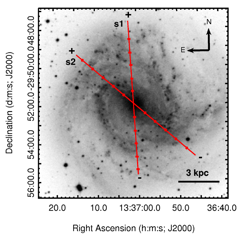
Figure 1.— The two longslits overlaid on a red image of M83 from the Digitized Sky Survey (Second Generation; https://archive.stsci.edu/cgi-bin/dss_form). The tickmarks indicate galactocentric radii of $|R|=1-5$ kpc, and the plus and minus signs show the sides of the galaxy with positive and negative $R$, respectively.

During each night of observations, we obtained a single separate sky exposure that approximates the track followed by the telescope during the science exposures, and scaled the former by a multiplicative factor to account for variations in sky brightness. After sky subtraction, we combined the spectra within, and then between, nights; to do so, we scaled the spectra by their median values, stacked them by their median once again, and extracted them using an aperture of 11 pixels. The aperture width was chosen to be large enough to minimize the effect of curvature of the spatial axis with respect to the pixel rows and to gain in signal-to-noise (S/N) without significantly sacrificing the spatial resolution. We calculated the error bars from the rms uncertainty in the continuum assuming that the S/N scales according to Poisson statistics ($\sqrt{N}$). Vignetting of as much as 25$\%$ of the slit required cropping of some frames before stacking, reducing the S/N at the ends of the slits.

2.1. Flux Calibration

We perform the relative flux calibration using observations of the spectrophotometric standard star Hiltner 600. Absolute flux calibration is not possible with SALT alone due to the varying effective telescope area as a function of time. Thus, to perform the flux calibration, we use Hubble Space Telescope (HST) Wide Field Camera 3 imaging of M83 from the Hubble Legacy Archive (PI: Blair; Proposal ID: 12513). The images are taken with the f657n narrow-band filter; at the redshift of M83, the filter window includes the [NII]$\lambda\lambda$6548, 6583 and H$\alpha$ lines. The image mosaic covers $\sim 100\%\text{ and }75\%$ of the spatial extents of slits 1 and 2, respectively.

To perform the flux calibration, we convolved the HST mosaic with a two-dimensional Gaussian using the IDL function gauss smooth. The standard deviation of the Gaussian kernel was equal to the estimated seeing at the SALT site, $\sigma=1.5"$. For each section of the slit from which a spectrum was extracted, we calculated the average flux density required to produce the observed HST counts using the PHOTFLAM keyword. Accounting for the filter throughput, we then determined the average flux density of the SALT spectra to yield a conversion factor between instrumental and astrophysical units at H$\alpha$.

Due to saturation and scattered light in the nucleus, and vignetting at the ends of the slits, we calculated a median conversion factor, $f$, for spectra between $1\text{ kpc}\leq|R|\leq 4\text{ kpc}$. This yielded $f=2.1\pm 0.4\times 10^{-16}\text{ erg cm}^{-2}\text{ SALT ADU}^{-1}$ for slit 1 and $f=2.3\pm 0.4\times 10^{-16}\text{ erg cm}^{-2}\text{ SALT ADU}^{-1}$ for slit 2, suggesting that the flux calibration is accurate to $\sim 20\%$.

2.2. Instrumental Scattered Light

Within $\sim 40"$ ($|R|=1$ kpc) of the center, an instrumental scattered light feature appears as very broad emission ($\sigma=0.5-1\times 10^{3}$  km s^-1) under the H$\alpha$ and [NII]$\lambda\lambda$6548, 6583 emission lines. This feature is most noticeable in the moderate spectral resolution data at $|R|=1$ kpc, where its intensity becomes comparable to the H$\alpha$ intensity. To verify that it is due to instrumental scattered light, we obtained another RSS longslit observation using the same instrument setup, and adjusted the pointing center (R.A. = 13 37 01.9, Decl. = -29 52 13, J2000) and position angle (P.A. = 28^∘) to avoid the brightest part of the nucleus. The absence of the broad emission feature from this observation suggests that it is due to instrumental scattered light from bright nuclear star clusters.

We simultaneously remove the scattered light and the continuum by masking the emission lines, smoothing with a Gaussian filter, and subtracting the result. At low spectral resolution, we use a Gaussian window with $\sigma=12.5$ Å. At moderate spectral resolution, we choose $\sigma=25$ Å and $\sigma=10$ Å; the latter is used where the scattered light intensity is comparable to the H$\alpha$ intensity. These choices produce sufficiently smooth continua while capturing the curvature of the scattered light emission where necessary. We assume no additional error associated with the scattered light and continuum subtraction.

3. Detection of Multiple Emission-Line Components: A Markov Chain Monte Carlo Method

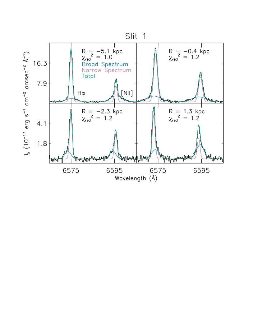
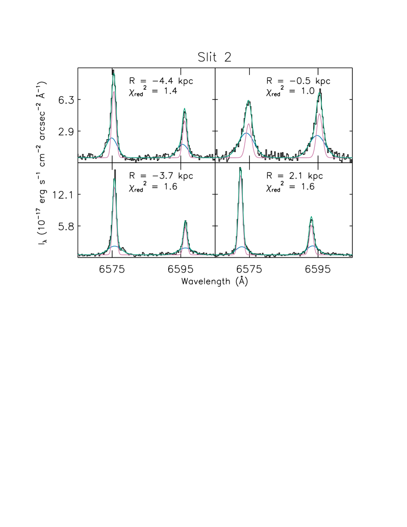
Figure 2.— Example spectra from slits 1 (top) and 2 (bottom) showing a Gaussian decomposition into a narrow (pink) and broad (blue) component. A Markov Chain Monte Carlo method was used to decompose the [NII]$\lambda\lambda$6548, 6583, H$\alpha$, and [SII]$\lambda\lambda$6717, 6731 emission lines into multiple components; for clarity, only the H$\alpha$ and [NII]$\lambda$6583 lines are shown here. The spectra shown are chosen to illustrate the range of emission line intensities, morphologies, and ratios observed in each component.

Table 2Markov Chain Monte Carlo Parameters

	$I(H\alpha)_{b}/I(H\alpha)_{tot}$	[NII]$\lambda$6583/H$\alpha|_{b}$	[SII]$\lambda$6717/H$\alpha|_{b}$	[SII]$\lambda$6731/H$\alpha|_{b}$	$v_{n}$	$v_{b}$	$\sigma_{n}$	$\sigma_{b}$
					km s-1	km s-1	km s-1	km s-1
Initial Value	0.25	1.0	0.5	0.5	500	500	30	50
Step Size	0.1	0.1	0.1	0.1	10	10	10	10

Our first goal is to identify multiple emission-line components. Using the moderate spectral resolution data, we model the [NII]$\lambda\lambda$6548, 6583, H$\alpha$, and [SII]$\lambda\lambda$6717, 6731 emission lines as a superposition of two Gaussians, and ask whether these components are consistent with arising from eDIG, planar DIG (pDIG), or HII regions. To do so, we use the following criteria: 1) The [NII]$\lambda$6583/H$\alpha$ and [SII]$\lambda$6717/H$\alpha$ emission-line ratios are higher in diffuse gas than in HII regions (e.g., Rand, 1998; Otte et al., 2002; Madsen et al., 2006), 2) the velocity dispersion in diffuse gas may be higher than in HII regions (Heald et al. 2006b, a, 2007; B16), and 3) eDIG may display a rotational velocity lag with respect to the HII regions in the disk (e.g., Fraternali et al., 2004; Heald et al., 2006b, a, 2007; Bizyaev et al., 2017). Since adding additional Gaussians will almost always improve the quality of the fit, these considerations are crucial to tie the Gaussian decomposition to the underlying physical processes. Note that here and throughout the rest of this paper, HII region emission refers not only to that from individual Strömgren spheres, but also to that from the planar, dense, ionized gas found locally in star-forming regions.

We use a Markov Chain Monte Carlo (MCMC) method with a Metropolis-Hastings algorithm to model the emission-line profiles as the sum of a narrow and a broad component (e.g., Ivezić et al., 2014). We probe an 8-dimensional parameter space defined by the broad H$\alpha$ intensity, [NII]$\lambda$6583/H$\alpha$, [SII]$\lambda$6717/H$\alpha$, and [SII]$\lambda$6731/H$\alpha$, as well as the broad and narrow velocities and velocity dispersions. To prevent degeneracies in parameter space, we require that the velocity dispersion of the narrow component not exceed that of the broad. We assume that the velocity dispersions do not depend on atomic species; as we will see in §4.2, this is a reasonable assumption since the turbulent contribution dominates the thermal contribution. We also assume that [NII]$\lambda$6548/[NII]$\lambda$6583 = 0.3 for both the broad and narrow component, but do not make an assumption about the value of [SII]$\lambda$6717/[SII]$\lambda$6731. We require that the sum of the narrow and broad intensities equal the observed, integrated intensity. The analysis is only performed if at least three of the five emission lines are detected at the 5$\sigma$ level.

For a given spectrum, the MCMC method is implemented as follows. First, we chose a location in parameter space, construct a model, and quantify the quality of the fit using the $\chi^{2}$ statistic:

$$\chi^{2}=\sum_{n}\frac{(f_{\lambda,obs}-f_{\lambda,mod})^{2}}{\sigma_{obs}^{2}},$$ (1)

where $f_{\lambda,obs}$ and $f_{\lambda,mod}$ are the observed and modeled flux densities, $\sigma_{obs}$ is the observed uncertainty, and $n$ is the number of wavelength bins. We calculate the value of $\chi^{2}$ within 8 Å of the center of the emission lines of interest.

Next, we select a parameter from a uniform distribution. We then select a distance and direction to move in that parameter from a Gaussian distribution with a standard deviation equal to a given step size. The decision to accept or reject this new model is based on an acceptance probability given by:

$$p=\text{e}^{-(\chi_{new}^{2}-\chi_{old}^{2})/2},$$ (2)

where $\chi_{new}^{2}$ and $\chi_{old}^{2}$ give the quality of the fit of the new and old models, respectively. If $p>1$, the new model is accepted as a better fit. If $p<1$, the value of $p$ is compared to a number $n$ from a uniform distribution where $0\leq n\leq 1$. If $p>n$, we accept the new model. Likewise, if $p<n$, we reject the new model in favor of the old. This ensures that a new model is always accepted when it provides a better fit, and is sometimes accepted when it doesn’t to ensure sufficient sampling of parameter space.

This process is repeated for $N=10^{5}$ links in the MCMC chain; our choice of $N$ is discussed in Appendix A, where we demonstrate the convergence of the algorithm. The first $10^{4}$ links are rejected as the “burn-in”. The remaining links are used to construct distributions of the accepted values of each parameter. The median values of the distributions are taken as the parameter values, and the median absolute deviations are taken as the parameter uncertainties. In Table 2, we show the starting values and step sizes of each parameter. The results are not sensitive to either the start values or the step sizes; however, we select the step sizes to achieve an acceptance fraction of $<50\%$ to ensure effective sampling of the parameter space.

As a check on our parameter uncertainties, we randomly perturb each flux bin in every spectrum by adding or subtracting the one-sigma error bar. We then run the same MCMC algorithm on the perturbed data, and compare the best-fit parameters from the perturbed and unperturbed data. The uncertainty estimate implied from this comparison exceeds that implied by the original MCMC analysis for all parameters. For most parameters, the effect is small ($10-30\%$); however, in some cases, it is as high as a factor of two. Thus, when considering the error estimates in this paper, it should be noted that they may be underestimated by factors in this range.

After the MCMC algorithm constructs a two-component model for each spectrum, we implement an additional criterion to identify the true two-component spectra. In cases where the emission lines are well-represented by a single Gaussian, the second Gaussian often fits to noise, structure in the continuum, or curvature caused by the H$\alpha$ stellar absorption feature. To identify true two-component spectra, we require that each component comprises at least 15$\%$ of the integrated intensity of at least 3 of the emission lines. Those without two-component spectra are fit with single Gaussians, yielding both multi-component (broad, narrow) and single-component fits. Of 388 total spectra, 350 spectra have 5$\sigma$ detections, and 191 and 159 spectra have multi- and single-component fits, respectively. The multi-component spectra are distributed across the full range of galactocentric radii considered.

In Figure 2, we show a comparison of the best-fit two-component modeled and observed spectra. By eye, the quality of the fits are very good, and the reduced $\chi^{2}$ values of the two-component fits have a median value of $\chi_{red}^{2}=1.4$. Due to the degeneracy of Gaussian decomposition, this approach cannot produce a unique decomposition for a given spectrum. However, taken in aggregate, the results reveal the physical conditions and kinematics in the narrow- and broad-line emitting regions. We discuss the properties of the narrow and broad components, and their relationship to eDIG, pDIG, and HII region emission, in the following section.

4. Observational Results

4.1. Identification of DIG Emission

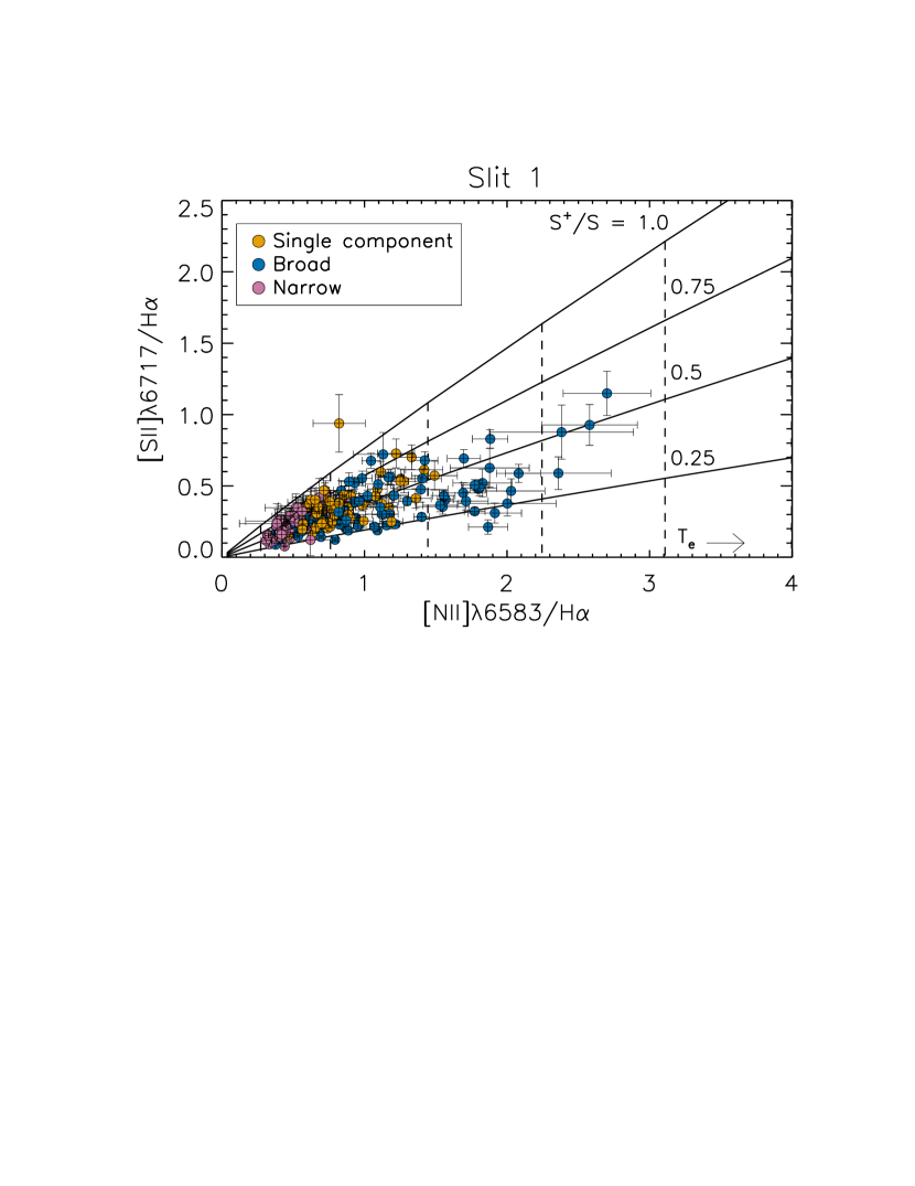
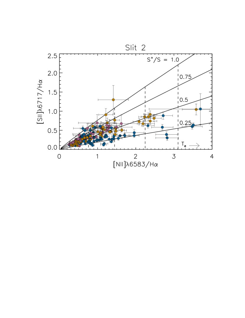
Figure 3.— The narrow (pink) and broad (blue) emission-line components from slits 1 (top) and 2 (bottom) lie in regions of the [NII]$\lambda$6583/H$\alpha$, [SII]$\lambda$6717/H$\alpha$ plane consistent with HII region and DIG emission, respectively. The solid lines correspond to a constant ionization fraction of $S^{+}/S=0.25,0.5,0.75,\text{and }1.0$ from bottom to top, and the dashed lines indicate a constant electron temperature of $T_{e}=0.6,0.8,1.0,1.2,\text{and }1.4\times 10^{4}$ K from left to right. The broad components lie largely at high ratios of forbidden line emission to recombination line emission suggestive of high temperatures ($0.8\times 10^{4}$ K $<T_{e}<1.4\times 10^{4}$ K) and ionization states ($S^{+}/S<0.75$). The single-component spectra (yellow) tend to arise from intermediate physical conditions; however, in slit 2, single-component fits with high [NII]$\lambda$6583/H$\alpha$ are found within $|R|<2$ kpc where there is evidence for shock ionization near star-forming regions (Calzetti et al., 2004; Hong et al., 2011). In slit 2, seven data points lie at [NII]$\lambda$6583/H$\alpha>4$.

In Figure 3, we compare the [NII]$\lambda$6583/H$\alpha$ and [SII]$\lambda$6717/H$\alpha$ emission-line ratios for the narrow, broad, and single-component spectra. We indicate the expected values of these emission-line ratios based on abundances, electron temperature, and ionization fraction as follows. The emission-line ratios can be expressed as:

$$\begin{split}\frac{I([NII]\lambda 6583)}{I(H\alpha)}=1.63\times 10^{5}\bigg{(}\frac{H^{+}}{H}\bigg{)}^{-1}\bigg{(}\frac{N}{H}\bigg{)}\bigg{(}\frac{N^{+}}{N}\bigg{)}\times\\ T_{4}^{0.426}\text{e}^{-2.18/T_{4}}\end{split}$$ (3)

and

$$\begin{split}\frac{I([SII]\lambda 6717)}{I(H\alpha)}=7.67\times 10^{5}\bigg{(}\frac{H^{+}}{H}\bigg{)}^{-1}\bigg{(}\frac{S}{H}\bigg{)}\bigg{(}\frac{S^{+}}{S}\bigg{)}\times\\ T_{4}^{0.307}\text{e}^{-2.14/T_{4}},\end{split}$$ (4)

where $T_{4}$ is the electron temperature in units of $10^{4}$ K (Haffner et al., 1999; Osterbrock & Ferland, 2006). We use $N/H=9.8\times 10^{-5}$ and $S/H=1.2\times 10^{-5}$ as median values of direct abundances determined from auroral lines detected in five HII regions by Bresolin et al. (2005, see their Table 12). We assume that the H and N are $100\%$ and $80\%$ ionized, respectively; in the Milky Way, $H^{+}/H>0.9$ for $T_{4}>0.8$ (Reynolds et al., 1998), and $N^{+}/N\sim 0.8$ under a range of DIG conditions (Sembach et al., 2000). Though $N^{+}/N$ is fairly constant in the DIG, $S^{+}/S$ may vary under these conditions, due to the different second ionization potentials of these species (23.3 eV for $S^{+}\rightarrow S^{2+}$, 29.6 eV for $N^{+}\rightarrow N^{2+}$).

In Figure 3, we allow both $T_{4}$ and $S^{+}/S$ to vary, indicating dashed lines of constant $T_{4}$ and solid lines of constant $S^{+}/S$. This analysis neglects, among other things, a radial abundance gradient and variations in abundances, ionization fractions, and electron temperature along the line of sight. However, it gives us a qualitative sense of the physical conditions from which the narrow and broad emission arise.

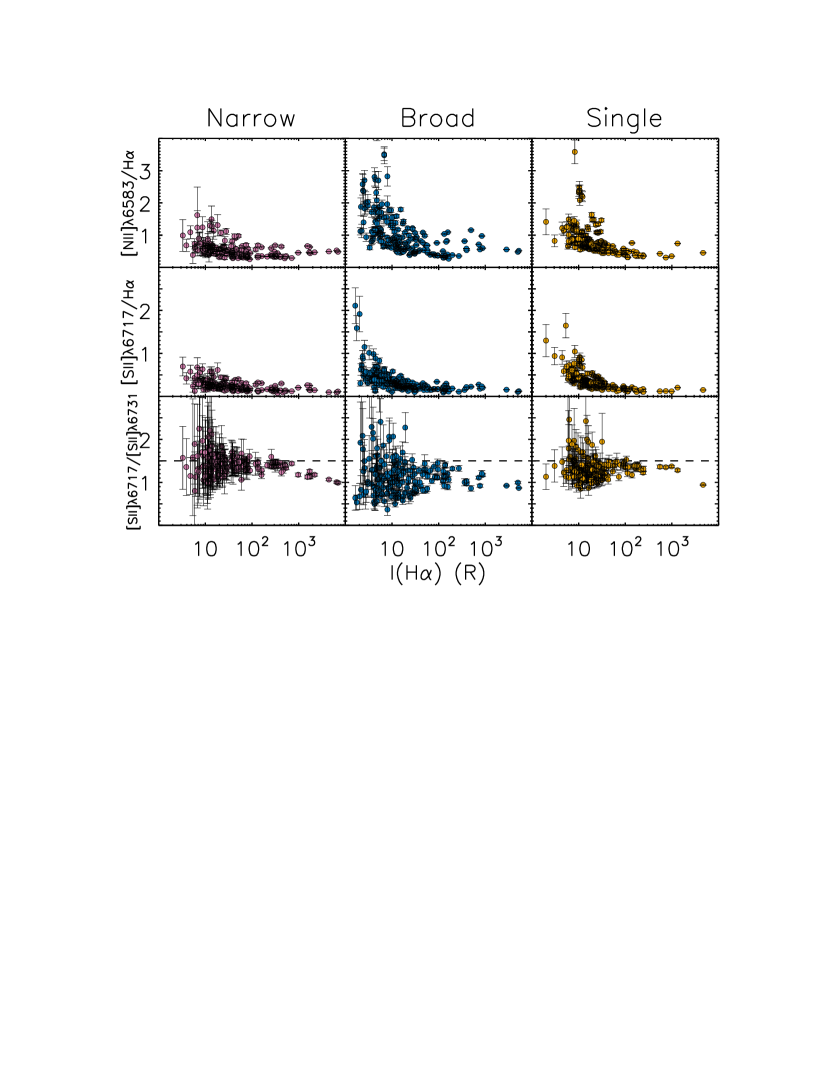
Figure 4.— [NII]$\lambda$6583/H$\alpha$ (top row), [SII]$\lambda$6717/H$\alpha$ (middle), and [SII]$\lambda$6717/[SII]$\lambda$6731 (bottom) as functions of $I(H\alpha)$ for the narrow (left), broad (center), and single-component (right) spectra. The surface brightness is corrected for the inclination of the galaxy. Top and middle rows: The broad emission tends to fall at fainter $I(H\alpha)$ and higher [NII]$\lambda$6583/H$\alpha$ and [SII]$\lambda$6717/H$\alpha$ than the narrow emission, consistent with arising from a more diffuse medium subject to supplemental heating (i.e., a heating mechanism proportional to $n_{e}^{\alpha}$, where $\alpha<2$). Bottom row: The narrow and single components are generally consistent with the low-density limit within the errors ([SII]$\lambda$6717/[SII]$\lambda$6731 $=1.5$, indicated by the dashed line). However, the broad component shows a much larger scatter in the line ratio; while measurements at $I(H\alpha)\geq 10^{2}\text{ R}$ may be indicative of dense shells in the starburst nucleus, those at $I(H\alpha)\leq 30\text{ R}$ are unreliable due to low S/N and possible instrumental effects.

In slit 1, the narrow emission lies at the lowest values of the emission-line ratios around [NII]$\lambda 6583$/H$\alpha\sim 0.5$ and [SII]$\lambda 6717$/H$\alpha\sim 0.3$ between $0.6\leq T_{4}\leq 0.9$. In contrast, the broad emission is scattered between $0.5\leq$ [NII]$\lambda 6583/$H$\alpha\leq 2.7$, $0.1\leq$ [SII]$\lambda 6717/$H$\alpha\leq 1.2$, and $0.7\leq T_{4}\leq 1.3$. Both components span a range in ionization fraction ($0.25\leq S^{+}/S\leq 1.0$). Thus, the narrow and broad emission are consistent with arising from HII regions and the warmer DIG in a metal rich galaxy; a similar behavior is seen for emission from HII regions and WIM in the Milky Way (e.g., Haffner et al., 1999). The single-component spectra show intermediate line ratios between $0.7\leq T_{4}\leq 1.0$, suggesting that these spectra originate from a range of physical conditions. Those with lower and higher emission-line ratios are likely dominated by HII region and DIG emission, respectively.

In slit 2, the spectra show a similar behavior, although considerably more single-component spectra lie at [NII]$\lambda 6583$/H$\alpha>1.5$, and more broad spectra are found at [NII]$\lambda 6583$/H$\alpha>2$. These spectra are largely found at $|R|<2$ kpc, where LINER-like emission-line ratios have been previously observed. This emission is likely due to shock ionization from stellar winds and supernovae near star-forming regions (Calzetti et al., 2004; Hong et al., 2011). As discussed in §2.2, this phenomenon is spatially coincident with instrumental scattered light, and it is possible that residuals from scattered light subtraction interfere with our ability to identify multiple components.

As shown in the top and middle rows of Figure 4, [NII]$\lambda 6583$/H$\alpha$ and [SII]$\lambda 6717/$H$\alpha$ increase as $I(H\alpha)$ decreases. Thus, the fainter, broad emission, with H$\alpha$ intensities largely between $1\text{ R}<I(H\alpha)<10^{2}\text{ R}$, has higher ratios of forbidden line to recombination line emission than the brighter, narrow emission with $10\text{ R}<I(H\alpha)<10^{3}\text{ R}$. This trend, observed in the Milky Way and other nearby, edge-on disk galaxies (e.g., Rand, 1998; Haffner et al., 1999), has been attributed to a supplemental heating mechanism at low electron density, $n_{e}$, proportional to $n_{e}^{\alpha}$ for $\alpha<2$ (i.e., proportional to a lower power of $n_{e}$ than photoionization heating, $n_{e}^{2}$). Note that bright, broad emission with low emission-line ratios is observed in the nucleus of M83, likely due to dense, planar gas surrounding star-forming regions.

In the bottom row of Figure 4, we compare the [SII]$\lambda$6717/[SII]$\lambda$6731 emission-line ratios of the narrow, broad, and single components as a function of $I(H\alpha)$. As expected, the narrow and single components are largely at the low-density limit of [SII]$\lambda$6717/[SII]$\lambda$6731 $=1.5$. For $I(H\alpha)>10^{2}$, the broad component has [SII]$\lambda$6717/[SII]$\lambda$6731 $\sim 1$, consistent with electron densities of $n_{e}=10^{2}-10^{3}\text{ cm}^{-3}$ (Osterbrock & Ferland, 2006). This may be indicative of dense shells and filaments associated with the nuclear starburst. At $I(H\alpha)\leq 30\text{ R}$, there is significant scatter in [SII]$\lambda$6717/[SII]$\lambda$6731, and we do not trust the measured line ratios in this regime. The S/N is insufficient to robustly measure the line ratios at these intensities, and the results may be influenced by instrumental effects. A high S/N measurement of [SII]$\lambda$6717/[SII]$\lambda$6731 at faint $I(H\alpha)$ is of interest to determine if any of the broad emission originates from dense gas.

We do not correct for the H$\alpha$ stellar absorption line. The relative impact of absorption on the broad and narrow components is unclear. It is possible that absorption impacts the intensity of the narrow component more than the broad, as the former is more likely to be aligned with the stellar population in velocity space. Nevertheless, we estimate the impact of absorption if it exclusively impacts the broad and narrow components, respectively. Assuming an H$\alpha$ absorption line with an equivalent width of $EW=2$ Å, the H$\alpha$ absorption is generally comparable to the broad H$\alpha$ intensity, and ranges from comparable to smaller by several orders of magnitude for the narrow H$\alpha$ intensity. If the intensities are corrected for this absorption, the maximum observed line ratios are [NII]$\lambda$6583/H$\alpha\sim 1.5$ (0.5) and [SII]$\lambda$6717/H$\alpha\sim 0.4$ (0.3) for the broad (narrow) components.

In general, the broad component is consistent with arising from diffuse gas, while the narrow component is consistent with originating in HII regions. This is supported by the former components’ high [NII]$\lambda$6583/H$\alpha$ and [SII]$\lambda$6717/H$\alpha$ line ratios at faint $I(H\alpha)$. In the next section, we assess the kinematics of the narrow and broad components, and consider evidence for an eDIG layer.

4.2. Kinematics and Identification of eDIG Emission

In Figure 5, the line-of-sight velocity dispersion, $\sigma$, is shown as a function of $I(H\alpha)$. Here and throughout the rest of this paper, $\sigma$ refers to the standard deviation of the Gaussian fit. The velocity dispersion is corrected for instrumental resolution ($\sigma^{2}=\sigma_{obs}^{2}-\sigma_{res}^{2}$). The narrow emission generally has $10\text{\,km~{}s${}^{-1}$}<\sigma<30$  km s^-1, with a median value of $\sigma=20$  km s^-1, consistent with HII region line widths of a few tens of  km s^-1. Widths as large as $\sigma=50$  km s^-1are observed in the brightest narrow components from the turbulent, star-forming nucleus.

The broad component has a remarkable median velocity dispersion of $\sigma=96$  km s^-1, with a significant spread around this value of $40\text{\,km~{}s${}^{-1}$}<\sigma<150$  km s^-1. The moderate and large velocity dispersions of the narrow and broad components are suggestive of thin (planar) and thick (extraplanar) gaseous disks. With a median line width of $\sigma=26$  km s^-1, the single-component spectra have widths much more comparable to the narrow component than to the broad.

The heliocentric, line-of-sight velocities of the narrow, broad, and single components are shown as a function of galactocentric radius in Figure 6. The narrow and single components are dominated by the rotational velocity of the disk, but the broad component tends toward systemic velocity. The median difference in radial velocity between the narrow and the broad components implies a rotational velocity lag of $\Delta v=-24$  km s^-1in projection, or $\Delta v=-70$  km s^-1corrected for inclination.

This is qualitatively consistent with the rotational velocity lags that are characteristic of multi-phase, gaseous halos (e.g., Fraternali et al., 2002, 2004; Heald et al., 2006b, a, 2007; Oosterloo et al., 2007; Bizyaev et al., 2017), but is quantitatively in excess of the $\Delta v=-10--40$  km s^-1kpc^-1 commonly observed in nearby, edge-on eDIG layers (Heald et al., 2006b, a, 2007; Bizyaev et al., 2017). These lags are often interpreted as evidence of a galactic fountain; as gas clouds rise out of the disk, they experience a weaker gravitational field, move out in radius, and slow down to conserve angular momentum (e.g., Collins et al., 2002).

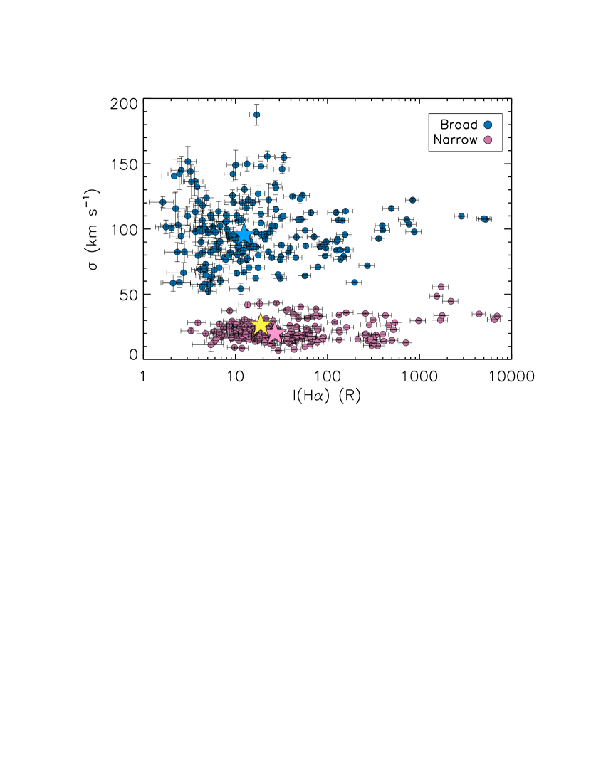
Figure 5.— The line widths of the broad components (blue) greatly exceed those of the narrow components (pink), suggesting that the former originates from a thicker gaseous disk. The median values of $\sigma$ and $I(H\alpha)$ for the broad ($\sigma=96$  km s^-1), narrow ($\sigma=20$  km s^-1), and single ($\sigma=26$  km s^-1) components are shown with the blue, pink, and yellow stars, respectively. The brightest, broadest narrow components at $I(H\alpha)\geq 10^{3}$ R originate in the nucleus. The individual single-component spectra are not shown for visual clarity. The line widths are corrected for the instrumental resolution, and the surface brightness is corrected for the inclination of the galaxy.

There is also evidence of local bulk flows in the broad component. In slit 1, outflows are suggested by the blueshifted gas near the nucleus ($-1\text{ kpc}<R<0\text{ kpc}$) and on the northeast side of the galaxy ($3\text{ kpc}<R<4\text{ kpc}$). The most remarkable local feature in slit 2 is at $R=-4$ kpc, where coherent, redshifted velocities arise where the slit crosses a star-forming spiral arm. These features may be due to expanding or collapsing shells or other local bulk motions characteristic of a galactic fountain flow.

One may ask whether the velocity profile of the broad component can be explained by a series of local bulk flows alone. However, this requires a preferential blueshifting and redshifting of the gas on the receding and approaching sides of the galaxy, respectively. Lacking a physical basis for this bias, the velocity profile is likely due to a lagging halo punctuated by local bulk flows. In general, the large velocity dispersion, rotational velocity lag, and local inflow and outflow are consistent with the broad emission arising from an eDIG layer.

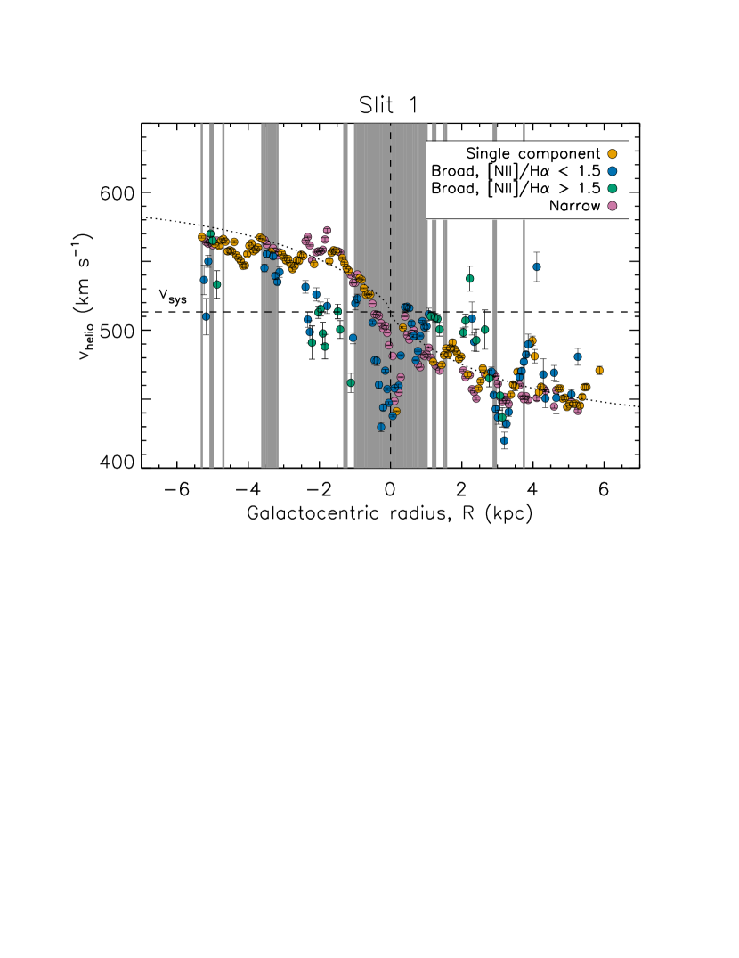
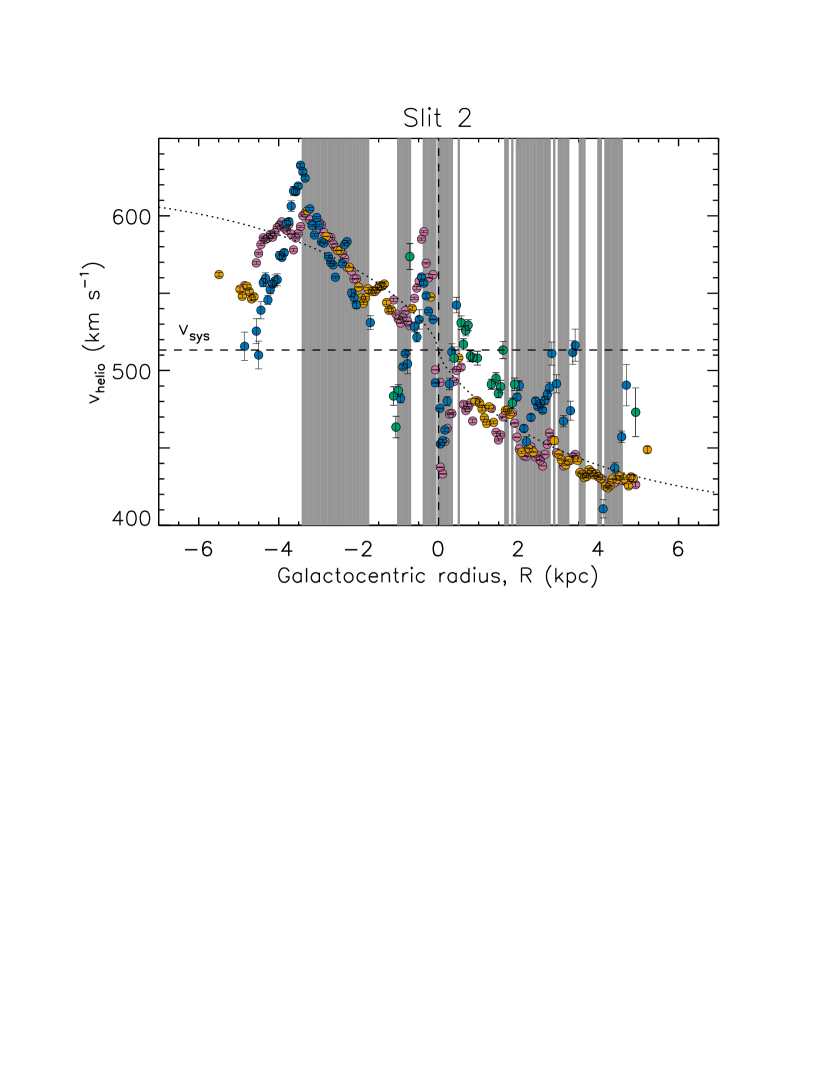
Figure 6.— For slits 1 (top) and 2 (bottom), the heliocentric radial velocities are shown for the narrow (pink), broad (blue and green), and single-component (yellow) spectra as functions of galactocentric radius. Broad emission with [NII]$\lambda 6583$/H$\alpha<1.5$ and with [NII]$\lambda 6583$/H$\alpha>1.5$ are shown in blue and green, respectively. Our best-fit rotation curve for M83 is shown by the dotted lines (see Appendix B), and the systemic velocity, $v_{sys}=513$  km s^-1, is indicated by the dashed lines. The shaded radii indicate regions of star-formation activity (see §4.3). In general, the broad component tends toward systemic velocity, suggesting an extraplanar gas layer with decreasing rotational velocity as a function of height above the disk. There is also evidence of local bulk flows; for example, in slit 1, a bulk blueshifting of the gas is seen near the nucleus ($-1\text{ kpc}<R<0\text{ kpc}$) and near $R=3$ kpc.

4.3. Proximity of eDIG Detection to Star-Formation Activity

Here, we evaluate the proximity of eDIG detection to star-formation activity in the disk. In doing so, we ask where the broad component truly arises from eDIG emission, and where it is due to pDIG emission associated with star-forming spiral arms.

We consider an observation to be from a star-forming region if the narrow $I(H\alpha)$ is at least three times higher than the minimum observed $I(H\alpha)\sim 10$ R. In Figure 7, we shade the galactocentric radii that meet this criterion. In the top panels, we show the broad $I(H\alpha)$ as a function of $R$. It is clear that the faintest emission is detected away from star-forming regions. $I(H\alpha)$ increases by several orders of magnitude in the starburst nucleus, and by factors that range from a few to an order of magnitude near star formation at larger $R$. This is a consequence of the $n_{e}^{2}$ dependence of the H$\alpha$ intensity; if a bright, planar component of the DIG exists along the line of sight, it will dominate the broad emission-line profile and compromise our ability to detect a fainter, extraplanar component along the same line of the sight.

In the bottom panels, we show the broad [NII]$\lambda 6583$/H$\alpha$ as a function of $R$. The highest values of [NII]$\lambda 6583$/H$\alpha$ that are indicative of the most diffuse gas are found between areas of star-formation activity. This again suggests that the broad component is dominated by pDIG emission near areas of star formation, and by eDIG emission elsewhere.

To confirm an eDIG detection, we must also consider the gas kinematics. In Figure 6, we shade the star-forming regions on the position-velocity diagrams, and we distinguish between broad emission in two emission-line ratio regimes. The most diffuse, broad emission with [NII]$\lambda 6583$/H$\alpha>1.5$ is shown in green, and the rest of the broad emission is shown in blue. In general, the most diffuse emission tends toward systemic velocity, consistent with a warm, ionized component of a lagging halo. The less diffuse emission shows a range of kinematics; in some places, it is consistent with the velocity of the disk, while in others it tends toward systemic velocity or appears to be locally inflowing or outflowing.

In summary, the broad component arises from diffuse gas with a range of densities and proximities to sources of ionizing radiation. Away from star-forming regions, we detect broad emission with the clearest signature of extraplanar, diffuse gas: faint $I(H\alpha)$, high values of [NII]$\lambda 6583$/H$\alpha$, and a rotational velocity lag with respect to the disk. Close to star-formation activity, the broad emission is suggestive of planar, diffuse gas or the base of the eDIG layer: brighter $I(H\alpha)$, lower values of [NII]$\lambda 6583$/H$\alpha$, and more complex kinematics that include rotation with the disk and local bulk flows. This result does not preclude the possibility of an eDIG layer found above both star-forming and quiescent regions. However, we cannot detect extraplanar emission along lines of sight dominated by bright, broad, planar emission with the methods used here.

Note that the line width of the broad component does not show a clear trend with $I(H\alpha)$, emission-line ratios, or line-of-sight velocity, so we take the median line width of the broad emission as the velocity dispersion of the eDIG layer for the remainder of this paper.

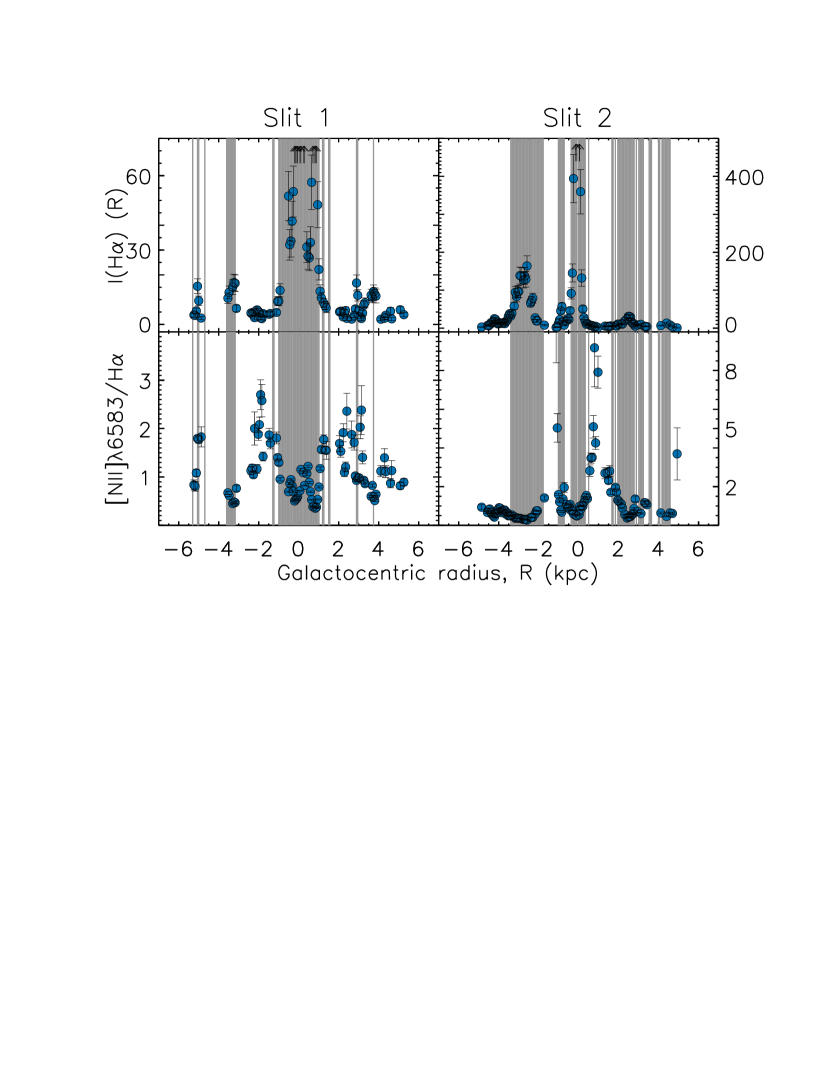
Figure 7.— The H$\alpha$ intensities and [NII]$\lambda 6583$/H$\alpha$ emission-line ratios of the broad component as functions of galactocentric radius, where shaded radii indicate regions of star-formation activity ($I(H\alpha)\geq 30\text{ R}$ in the narrow component). The broad emission is characteristic of an eDIG layer away from star-forming regions, where $I(H\alpha)$ is faintest and [NII]$\lambda 6583$/H$\alpha$ is highest. Likewise, the broad emission is suggestive of planar gas or of the base of the eDIG layer near star-formation activity. Here, $I(H\alpha)$ is brighter by factors that range from a few to several orders of magnitude, and [NII]$\lambda 6583$/H$\alpha$ is intermediate between values observed in HII regions and in diffuse gas. Arrows indicate radii with $I(H\alpha)$ values that exceed the figure range.

5. Mass of eDIG Layer

We estimate the mass of the eDIG layer using the H$\alpha$ surface brightness to assess the relative importance of the various phases of the gaseous halo. The H$\alpha$ surface brightness is related to the electron density by:

$$I(H\alpha)=\frac{\int\phi n_{e}^{2}\text{d}l}{2.75T_{4}^{0.9}},$$ (5)

where $\phi$ is the volume filling factor and $\int\text{d}l=L$ is the pathlength through the gas. Here, $I(H\alpha)$ is in Rayleighs, and $\text{d}l$ is in parsecs. We have corrected $I(H\alpha)$ for inclination assuming an optically thin disk, and thus the line of sight is taken to be perpendicular to the disk.

We estimate the characteristic surface brightness of the most diffuse eDIG detected, $I(H\alpha)=5.6$ R, by taking the median surface brightness at $|R|\geq 1$ kpc in slit 1 (see Figure 7). Assuming $I(H\alpha)=5.6$ R, $T_{4}=1$, $L=1$ kpc, and no variation in the physical conditions along the line of sight, we find $n_{e}=0.1\text{ cm}^{-3}$ and $n_{e}=0.4\text{ cm}^{-3}$ for $\phi=1$ and $\phi=0.1$, respectively. Our choice of $L=1$ kpc follows from the characteristic scale height of the eDIG layer in the Milky Way and nearby edge-on disk galaxies (e.g., Rand, 1997; Haffner et al., 1999; Collins & Rand, 2001).

If the eDIG layer extends no farther than the slits ($|R|=6$ kpc), and is a uniform disk of height $L=1$ kpc, then the total mass in the eDIG is $M_{eDIG}=8\times 10^{8}\text{ M}_{\sun}$ ($M_{eDIG}=3\times 10^{8}\text{ M}_{\sun}$) for $\phi=1$ ($\phi=0.1$). This likely underestimates the total mass, as increased values of $I(H\alpha)$ suggest higher values of $n_{e}$ near star-forming regions. Although this is a rough estimate subject to assumptions about the geometry of the layer, the volume filling factor, and the variation in physical conditions along the line of sight, it is consistent with estimates of the eDIG mass in other galaxies (e.g., Dettmar, 1990).

6. A Dynamical Equilibrium Model

We now turn to the second goal of this work, to test a dynamical equilibrium model of the eDIG layer in M83. We ask whether there is sufficient support available in thermal and turbulent pressure gradients to produce a scale height characteristic of these layers ($h_{z}=1$ kpc). Although, critically, additional support may be found in magnetic field and cosmic ray pressure gradients (e.g., B16), we lack information about these gradients in face-on galaxies, and thus do not consider them quantitatively here.

Our dynamical equilibrium model requires that force balance is satisfied in the vertical and radial directions in an axisymmetic disk:

$$\frac{\partial P(z,R)}{\partial z}=-\rho(z,R)\frac{\partial\Phi(z,R)}{\partial z},$$ (6)

$$\frac{\partial P(z,R)}{\partial R}=\rho(z,R)\frac{v_{\phi}(z,R)^{2}}{R}-\rho(z,R)\frac{\partial\Phi(z,R)}{\partial R}.$$ (7)

Here, $\frac{\partial\Phi}{\partial z}=g_{z}$ and $\frac{\partial\Phi}{\partial R}=g_{R}$ are the gravitational accelerations in the $z$ and $R$ directions, respectively. We construct a mass model of M83 and determine the galactic gravitational potential in Appendix B. $P=P_{th}+P_{turb}$ is the sum of the thermal and turbulent pressures, $\rho$ is the gas density, and $v_{\phi}$ is the azimuthal velocity. Note that we do not include magnetic or cosmic ray pressure, magnetic tension, or viscosity in our analysis.

We assume an equation of state of the form

$$P(z,R)=\sigma^{2}(z)\rho(z,R),$$ (8)

where $\sigma^{2}=\sigma_{th}^{2}+\sigma_{turb}^{2}$ is the quadrature sum of the thermal and turbulent velocity dispersions. Here, the turbulent velocity dispersion refers broadly to random motions, and not to a specific description of turbulence. The observed velocity dispersion shows only local variations with $R$, and thus we considered only variations in $z$ below.

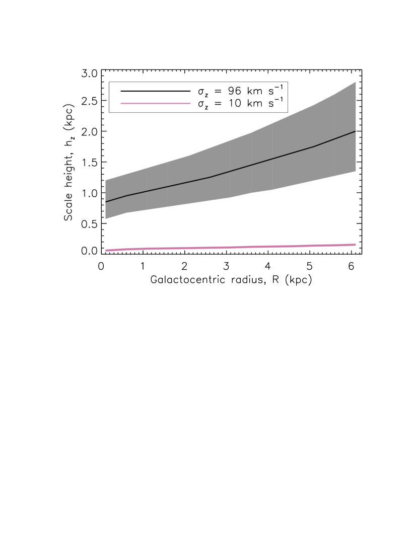
Figure 8.— The scale height, $h_{z}$, of an isothermal eDIG layer in the galactic potential of M83. The black and pink lines show $h_{z}$ for $\sigma=96$  km s^-1and $\sigma=10$  km s^-1, the median observed velocity dispersion and the sound speed in the eDIG, respectively. The shaded region shows the spread in $h_{z}$ that corresponds to the standard deviation in the observed velocity dispersion ($\sigma_{\sigma}=22$  km s^-1). If the observed velocity dispersion is indicative of a turbulent, cloud-cloud dispersion, then there is sufficient support in random motions to produce a characteristic eDIG scale height of $h_{z}\geq 1$ kpc.

Using the equation of state given in Equation (8), we solve Equation (6) to determine a general solution for the vertical density profile of the eDIG layer:

$$\frac{\rho(z,R)}{\rho(0,R)}=\frac{\sigma^{2}(0)}{\sigma^{2}(z)}\text{exp}\bigg{\{}-\int_{0}^{z}\bigg{(}\frac{\text{d}z^{\prime}}{\sigma^{2}(z^{\prime})}\frac{\partial\Phi(z^{\prime},R)}{\partial z^{\prime}}\bigg{)}\bigg{\}}.$$ (9)

If $\sigma$ is independent of $z$, we find the simplified solution below:

$$\rho(z,R)=\rho(0,R)\text{exp}\{-\sigma^{-2}(\Phi(z,R)-\Phi(0,R))\}.$$ (10)

We define the scale height of the eDIG layer, $h_{z}$, as the value of $z$ at which $\rho(h_{z})/\rho(0)=\text{e}^{-1}$. Thus, the scale height satisfies the condition:

$$\sigma^{2}=\Phi(h_{z},R)-\Phi(0,R).$$ (11)

In Figure 8, we show the scale height of an eDIG layer with a range of velocity dispersions in the galactic potential of M83. The scale height of a layer with the median observed $\sigma=96$  km s^-1reaches $h_{z}=1$ kpc by $R=1$ kpc. This is in contrast to the scale height produced by the sound speed in a $T\sim 10^{4}$ K gas ($\sigma\sim 10$  km s^-1), as the thermal scale height reaches only $h_{z}=0.15$ kpc within $R=6$ kpc. Thus, if the median observed $\sigma=96$  km s^-1is characteristic of a constant, cloud-cloud velocity dispersion throughout the eDIG layer, then there is sufficient support in thermal and turbulent motions to produce a scale height of $h_{z}\geq 1$ kpc.

We now consider the implications for the azimuthal velocity, $v_{\phi}$, of an eDIG layer with a constant velocity dispersion. By taking the partial derivatives of Equations (6) and (7) with respect to $R$ and $z$, respectively, subtracting the latter from the former, and re-expressing partial derivatives of $P$ in terms of partial derivatives of $\Phi$, we find that

$$0=\frac{-2v_{\phi}\rho(z,R)}{R}\frac{\partial v_{\phi}}{\partial z}.$$ (12)

Thus, for $\sigma$ constant with $z$, we find $\frac{\partial v_{\phi}}{\partial z}=0$. This model requires that there is no rotational velocity lag with respect to the disk, a consequence of the Taylor-Proudman theorem (e.g., Shore, 1992). For a polytropic equation of state, the Taylor-Proudman theorem states that there is no variation in the gas motions on a vertical column around the rotational axis. Thus, the gas motions are defined in the galactic disk, and there is no variation with height above the disk. The observation that the radial velocity of the eDIG emission tends toward systemic velocity is not consistent with this class of models.

In Appendix C, we allow $\sigma$ to vary with $z$, and we solve for the $\sigma(z)$ that satisfies the observed rotational velocity lag, $\frac{\partial v_{\phi}}{\partial z}$. We find, in summary, that an increase in $\sigma$ as a function of $z$ is required to reproduce $\frac{\partial v_{\phi}}{\partial z}$, but the magnitude of the increase is highly sensitive to $\epsilon=\sqrt{R\frac{\partial\Phi(h_{HI})}{\partial R}}-v_{\phi}(h_{HI})$, the difference between the circular velocity and the eDIG velocity at the HI scale height. Due to the need to fine-tune this dynamical equilibrium model, and the evidence for local bulk flows near star-forming regions, we favor a quasi- or non-equilibrium model.

7. Discussion

Here, we discuss our results in the context of multi-wavelength observations of M83 and similar systems, and compare our observations with the predictions of dynamical equilibrium and non-equilibrium models.

7.1. A Multi-Phase Gaseous Halo

There is observational evidence for a multi-phase, gaseous halo in M83 (see §1). There are similarities in the extraplanar HI and eDIG properties. Both phases have rotational velocity lags of a few tens of  km s^-1in projection; however, the velocity dispersions differ by almost an order of magnitude. Thus, it is difficult to characterize the relationship between the diffuse and neutral phases at the disk-halo interface. A model in which the two phases are directly related - for example, in which the eDIG forms a “skin” on condensing, neutral clouds - predicts a comparable velocity dispersion for the warm and neutral phases. However, as the neutral velocity dispersion may be underestimated, we cannot rule out such a model. Our eDIG mass estimate exceeds the extraplanar HI mass by an order of magnitude. This suggests that the former is the dominant phase relative to the latter, or that the former has a very small volume filling factor.

Perhaps the more revealing comparison is between the kinematics of the hot halo and the eDIG layer. The velocity dispersion of the latter is consistent with the sound speed in the former, suggesting that the velocity dispersion is inherited from the hot phase, possibly via entrainment or condensing clouds. Additionally, the eDIG emission blueshifted with respect to the disk within $R=1$ kpc may be produced by warm gas entrained in a hot outflow. However, due to the kinematics of the bar, the eDIG and disk velocities are difficult to characterize in this region. The LINER-like emission-line ratios observed near the nucleus in this work, Calzetti et al. (2004), and Hong et al. (2011) may be produced by a nuclear outflow shocking the surrounding, planar DIG layer.

7.2. Comparison to Other Galaxies

We can compare the eDIG properties and kinematics in M83 with that in the Milky Way and nearby, edge-on disk galaxies. The faintest emission detected in M83 is an order of magnitude brighter than that observed in the Milky Way by the Wisconsin H-Alpha Mapper survey (e.g., Haffner et al., 1999, 2003). Thus, we are not sensitive to the most diffuse component of the eDIG in M83, as the dependence of the H$\alpha$ intensity on the square of the electron density biases us toward the densest gas along the line of sight. This is an important consideration as we compare eDIG properties across galaxies with a range of inclination angles.

In nearby, edge-on disk galaxies, rotational velocity lags of a few tens of  km s^-1kpc^-1 are observed in eDIG layers (e.g., Heald et al., 2006b, a, 2007; Fraternali et al., 2004; Bizyaev et al., 2017). Assuming that we are detecting the densest eDIG closest to the disk, the observed median velocity lag of $\Delta v=-70$  km s^-1deprojected is steeper than the $\Delta v\sim-15--25$  km s^-1per scale height observed in other systems (Heald et al., 2007). However, without a measurement of the scale height in M83, it is difficult to make a strong statement about the steepness of the rotational velocity gradient.

The more striking comparison is the velocity dispersion of the eDIG layers. In the Milky Way, a velocity dispersion of $\sigma(H\alpha)\sim 12$  km s^-1is observed toward the north Galactic pole (L. M. Haffner, private communication). In NGC 891, $\sigma(H\alpha)=27$  km s^-1above $z=1$ kpc (B16), and several similar systems have $\sigma(H\alpha)=40-60$  km s^-1, albeit at lower spectral resolution (Heald et al., 2006b, a, 2007). Fraternali et al. (2004) detect locally broadened H$\alpha$ emission in the moderately-inclined galaxy NGC 2403, with $\sigma(H\alpha)\leq 300$  km s^-1. However, the eDIG layer in M83 is an outlier, as we detect $\sigma(H\alpha)\sim 100$  km s^-1all along the slit, with little evidence for a dependence on underlying disk features.

There are several possible explanations for this discrepancy. First, we may not be measuring comparable quantities in all galaxies. In an edge-on galaxy, we may be quantifying $\sigma$ at higher $z$ than in a face-on galaxy; in the latter case, we can detect the densest eDIG closest to the disk, and the dependence of the H$\alpha$ intensity on the square of the electron density biases us toward this denser gas. Additionally, the velocity dispersion in eDIG layers may be anisotropic, resulting in discrepancies in the dispersions observed at a range of inclination angles. If so, this would be important for understanding eDIG dynamics, as the dispersions parallel to the disks are often assumed to be indicative of those perpendicular to the disks. It is also possible that the velocity dispersion scales with a galaxy property such as the star-formation rate. In future work, we will examine the relationship between vertical velocity dispersion and star-formation rate in face-on disk galaxies with a range of star-formation properties (Boettcher, Gallagher, & Zweibel, in preparation).

7.3. Comparison of Models

Here, we consider several models for the dynamical state of the eDIG layer in M83, and we discuss whether each is consistent with the observations. We pay particular attention to whether each model can explain the anomalously large $\sigma$ observed in this system.

A Dynamical Equilibrium Model: First, we consider the dynamical equilibrium model that we tested in §6. We found that we are able to reproduce the characteristic scale heights of eDIG layers ($h_{z}\sim 1$ kpc) from the observed velocity dispersion ($\sigma=96$  km s^-1). However, maintaining a reasonable energy requirement while reproducing the observed rotational velocity gradient requires fine-tuning of the model.

From our mass estimate in §5, the kinetic energy in random motions for $\sigma=96$  km s^-1is on the order of $KE\sim 10^{56}$ ergs. Following Draine (2011), the cooling time for a shock with $v_{s}\sim 100$  km s^-1in a medium with $n_{e}\sim 0.1$ cm^-3 is $t_{cool}\sim 7\times 10^{4}$ years. Thus, the cloud collision timescale must be long if the energy requirement is to remain reasonable. The likelihood of eDIG cloud collisions is reduced if this phase has a very small volume filling factor and is embedded in a hot halo. This suggests a picture in which the warm phase is condensing out of or evaporating into the hot phase, with a velocity dispersion that is characteristic of the sound speed in the hotter medium.

A Galactic Fountain Model: A galactic fountain flow describes the circulation of gas between the disk and the halo due to star-formation feedback (Shapiro & Field, 1976; Bregman, 1980). It is thought that the gas leaves the disk in a hot phase and returns to the disk after cooling, passing through a warm, ionized phase. However, it is not clear during which part of the cycle a warm ionized phase is present (e.g., whether warm gas is entrained in a hot outflow, or condenses from the hot phase).

The predictions of galactic fountain models include a rotational velocity gradient, local outflows from star-forming regions, and launch velocities around $\sim 100$  km s^-1(Shapiro & Field, 1976); all of these predictions are consistent with our observations. Additionally, a fountain flow that is largely in the $z$ direction is consistent with the smaller and larger $\sigma$ observed in high- and low-inclination galaxies, respectively. In this model, the large $\sigma$ results from local outflows near the disk as well as quasi-symmetric inflow and outflow near the turn-around height. The latter scenario is feasible due to the comparitively long time that a cloud spends at its maximum height, and is necessary to explain detections away from star-forming regions as well as the large $\sigma$ and $\partial v_{\phi}/\partial z$ observed along the same line of sight.

A Galactic Wind Model: The high X-ray surface brightness and the LINER-like emission-line ratios near the nucleus may be evidence of a hot, ionized outflow from the central kpc of M83. The eDIG within this region is largely blueshifted with respect to the disk, and may be entrained in an outflow. There is also evidence of local outflows from star-forming spiral arms. However, the eDIG layer at large does not appear to be associated with a galactic wind. The radial velocities are dominated by the rotational velocity of a lagging halo, and not by a preferentially blueshifted or redshifted flow. The relationship between the origin and evolution of eDIG layers and galactic outflows is of interest for further study.

An Accretion Model: We disfavor an accretion flow as the origin of the eDIG layer for several reasons. Firstly, the high [NII]$\lambda$6583/H$\alpha$ and [SII]$\lambda$6717/H$\alpha$ line ratios suggest that the gas is chemically enriched. If it is embedded in an accretion flow, the origin must be the enriched halo and not the pristine intergalactic medium. Secondly, the eDIG layer follows the rotation curve of the disk, albeit at a reduced rotational velocity. This is consistent with gas that originated in the disk, was lifted into the halo, and was radially redistributed to conserve angular momentum. However, the evidence for interaction in the extended HI disk of M83 should be kept in mind when considering the kinematics of the halo.

Thus, both a dynamical equilibrium model and a galactic fountain flow are broadly consistent with the observations. However, the need to fine-tune the former model leads us to favor the latter. The true dynamical state may be somewhere in between these models. Regardless, the importance of the hot (and potentially the cold) phase is clear, and emphasizes the need for a multi-wavelength approach to modeling these layers. For example, the mass hierarchy of hot, warm, and neutral gas suggested by this analysis may imply an energy flow: explusion of gas from the disk in the hot phase, condensation into clouds to produce the warm phase, and cloud-cloud collisions to cool to a neutral phase. The ability to address questions of energy balance and dynamics simultaneously is of interest for future work.

8. Summary and Conclusions

Using optical emission-line spectroscopy from the Robert Stobie Spectrograph on the Southern African Large Telescope, we performed the first detection and kinematic study of extraplanar diffuse ionized gas in the nearby, face-on disk galaxy M83. A Markov Chain Monte Carlo method was used to decompose the [NII]$\lambda\lambda$6548, 6583, H$\alpha$, and [SII]$\lambda\lambda$6717, 6731 emission lines into contributions from HII region, planar DIG, and extraplanar DIG emission. The eDIG layer is clearly identified by its emission-line ratios ([NII]$\lambda$6583/H$\alpha\mathrel{\hbox{\hbox to0.0pt{\hbox{\lower 4.0pt\hbox{$\sim$}}\hss}\hbox{$>$}}}1.0$), velocity dispersion ($\sigma=96$  km s^-1), and rotational velocity lag with respect to the disk. The main results are as follows:

• The median, line-of-sight velocity dispersion observed in the diffuse gas, $\sigma=96$  km s^-1, is a factor of a few higher than that observed in the Milky Way and nearby, edge-on disk galaxies. This suggests that the velocity dispersions in these layers may be anisotropic; however, further observations of the velocity dispersions in face-on eDIG layers are needed.

• The diffuse emission lags the disk emission in rotational velocity, qualitatively consistent with the multi-phase, lagging halos observed in other galaxies. The median velocity lag between the disk and the halo is $\Delta v=-24$  km s^-1in projection, or $\Delta v=-70$  km s^-1corrected for inclination. This exceeds the rotational velocity lags of $\Delta v\sim-15--25$  km s^-1per scale height observed in several nearby, edge-on disk galaxies (Heald et al., 2007).

• If the velocity dispersion is indicative of turbulent (random) motions, there is sufficient thermal and turbulent support to produce an eDIG scale height of $h_{z}\sim 1$ kpc in dynamical equilibrium. This model does not require vertical support from magnetic field or cosmic ray pressure gradients, consistent with a largely vertically-oriented (“X-shaped”) field. However, reproducing the observed velocity dispersion and rotational velocity gradient while keeping the energy requirement reasonable requires a finely tuned model.

• We favor a quasi- or non-equilibrium model for the eDIG layer. There is evidence of local bulk flows near star-forming regions that may trace the warm, ionized phase of a galactic fountain flow.

• Multi-wavelength observations of M83 reveal extraplanar hot and cold gas. The velocity dispersion of the eDIG layer is consistent with the sound speed in the hot phase, and rotational velocity lags are observed in both the cold and warm components. The relationship between the energetics and dynamics of these phases is of interest for future study.

In future work, we will construct a sample of both face-on and edge-on galaxies, develop a picture of the three-dimensional kinematics of eDIG layers, and contextualize this picture in the multi-phase environment of the disk-halo interface.

Appendix A Markov Chain Monte Carlo Convergence

Here, we discuss the convergence of the Markov Chain Monte Carlo method used in this work. We use $N=10^{5}$ links in the MCMC chain, and reject the first $N=10^{4}$ links as the “burn-in” period. In Figure 9, we demonstrate the convergence of the method at $N=10^{5}$ using all spectra from slit 1 with multi-component fits. For $N=1.25\times 10^{4},N=2\times 10^{4},N=5\times 10^{4},\text{ and }N=2\times 10^{5}$, we compare the normalized difference between the best-fit parameters at each $N$ and at $N=10^{5}$ ($\Delta P=|P(N)-P(N=10^{5})|/P(N=10^{5})$) with the normalized uncertainties on the best-fit parameters at $N=10^{5}$ ($\sigma_{P}(N=10^{5})/P(N=10^{5})$). We can conclude that the method has converged within the errors at $N=10^{5}$ if the former quantity is smaller than the latter at larger $N$. For $N=1.25\times 10^{4}$ and $N=2\times 10^{4}$, we find that $\Delta P>\sigma_{P}(N=10^{5})/P(N=10^{5})$ for 22% and 10% of the best-fit parameters, respectively. In comparison, for $N=5\times 10^{4}$ and $N=2\times 10^{5}$, this is reduced to an acceptable level of scatter at only 2%. Thus, the best-fit parameter values are largely unchanged within the uncertainties beyond $N=5\times 10^{4}$, and we conclude that the MCMC method is converged at our choice of $N=10^{5}$.

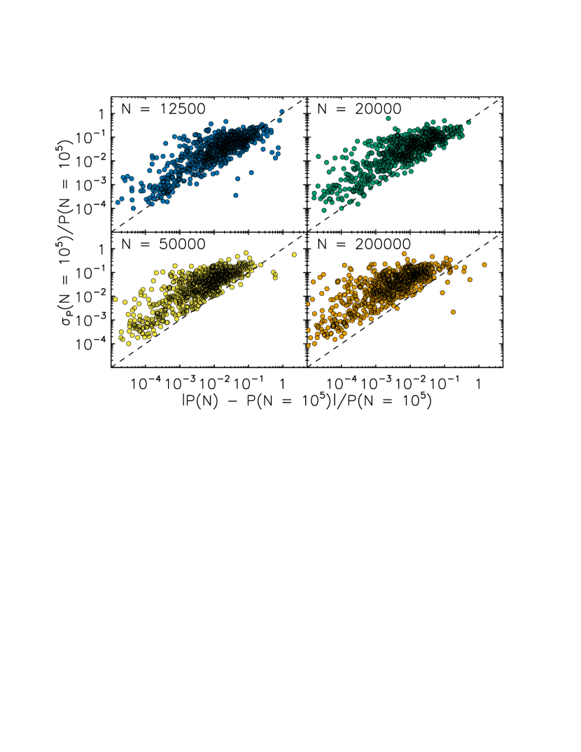
Figure 9.— The normalized difference between the best-fit parameters at $N$ and at $N=10^{5}$ links in the MCMC chain, $|P(N)-P(N=10^{5})|/P(N=10^{5})$ as compared to the normalized parameter uncertainties at $N=10^{5}$ ($\sigma_{P}(N=10^{5})/P(N=10^{5})$) for a range of $N$. Each point represents a best-fit parameter value for a spectrum in slit 1 with a multi-component fit. The dashed line denotes equality. For $N=5\times 10^{4}$ and $N=2\times 10^{5}$, only 2% of the best-fit parameter values vary with respect to $N=10^{5}$ by more than their uncertainties at $N=10^{5}$, suggesting that the MCMC method is converged within the errors for $N>5\times 10^{4}$. For all $N$, we reject the first $N=10^{4}$ links as the “burn-in” period.

Appendix B A Mass Model for M83

Here, we construct a mass model for M83 to determine the galactic gravitational potential. Herrmann & Ciardullo (2009) develop a mass model of the disk of M83 using the observed vertical velocity dispersion of planetary nebulae ($\sigma_{z,PNe}$) over a wide range of galactocentric radii ($R\leq$ 6 $R$-band scalelengths). The authors use a thin and thick disk model to reproduce the relatively flat distribution of $\sigma_{z,PNe}$ at large $R$. For both disks, they assume a vertical density distribution of the form:

$$\rho(z)=\rho_{0}\text{sech}^{2/n}\bigg{(}\frac{nz}{2h_{z}}\bigg{)}.$$ (13)

Here, $n=2$, as compared to the isothermal ($n=1$) and exponential ($n=\infty$) cases. Assuming exponential disks in $R$, the density distribution is the sum of the thin ($t$) and thick ($th$) components:

$$\begin{split}\rho(z,R)=\rho_{0,t}\text{e}^{-R/h_{R,t}}\text{sech}\bigg{(}\frac{z}{h_{z,t}}\bigg{)}+\rho_{0,th}\text{e}^{-R/h_{R,th}}\text{sech}\bigg{(}\frac{z}{h_{z,th}}\bigg{)}.\end{split}$$ (14)

The central velocity dispersions, $\sigma_{z}(0)$, vertical scale heights, $h_{z}$, and radial scale lengths, $h_{R}$, of these disk components are given in Table 3. For each component, we calculate central mass volume densities, $\rho_{0}$, from the central mass surface density, $\Sigma_{0}$, for $n=2$ disks: $\sigma_{z}^{2}(R)=1.7051\pi G\Sigma(R)h_{z}$. The total mass in the thin and thick disks is $5.8\times 10^{10}\mbox{\,$M_{\odot}$}$ and $3.6\times 10^{10}\mbox{\,$M_{\odot}$}$, respectively. Stellar mass estimates from Wide-field Infrared Survey Explorer (WISE) data suggest that this exceeds the baryonic mass by a factor of a few (Jarrett et al., 2013). This is a consequence of the low mass-to-light ratio required by Herrmann & Ciardullo (2009) to reproduce the relatively flat distribution in $\sigma_{z,PNe}$ as a function of $R$. Our goal is to quantify whether thermal and turbulent motions can support the eDIG layer at $h_{z}=1$ kpc. Thus, we favor an over-massive disk rather than an under-massive one, so that we may be sure that a successful model is not a result of underestimating the mass in the disk.

To reproduce the rotation curve, we add a dark matter halo with a Navarro-Frenk-White (NFW) profile of the form:

$$\rho_{DM}(R)=\frac{\rho_{0,DM}}{R/a_{DM}(1+R/a_{DM})^{2}},$$ (15)

where $\rho_{0,DM}$ is the central dark matter density and $a_{DM}$ is the scale radius. A range of inclination angles, $i$, and position angles, $PA$, have been suggested for M83, with evidence that the former increases and the latter decreases with $R$ (e.g., Huchtmeier & Bohnenstengel, 1981; Heald et al., 2016). We choose $i=24^{\circ}$ and $PA=226^{\circ}$, the smallest inclination determined for the inner disk, to once again favor the most massive model. With these assumptions, the HI rotation curve has a maximum velocity of $v_{c,max}\sim 255$  km s^-1between $R\sim 10-20$ kpc (Park et al., 2001; Heald et al., 2016).

We determine the values of $\rho_{0,DM}$ and $a_{DM}$ as follows. We test values of $a_{DM}$ between $1\text{ kpc}\leq a_{DM}\leq 30\text{ kpc}$; for each value of $a_{DM}$, we solve for the value of $\rho_{0,DM}$ that most closely produces $v_{c,max}=255$  km s^-1between $10\text{ kpc}\leq R\leq 20\text{ kpc}$. We then quantify the quality of the fit in a least-squares sense using our optical rotation curve for $R\leq 6$ kpc. The quality of the fit increases with increasing $a_{DM}$ at first, and then becomes fairly flat with increasing $a_{DM}$ beyond $a_{DM}=20$ kpc. Thus, we choose $a_{DM}=20$ kpc and $\rho_{0,DM}=6\times 10^{6}\mbox{\,$M_{\odot}$}\text{kpc}^{-3}$. We exclude velocities at $R\leq 0.5\text{ kpc}$ from this analysis due to the influence of the bar.

The gravitational potential of the thin and thick disks is of the form:

$$\begin{split}\Phi(z,R)=-\frac{4G\Sigma_{0}}{h_{R}}\int_{-\infty}^{\infty}\mathrm{d}z^{\prime}\,\Big{[}\text{sech}\bigg{(}\frac{z}{h_{z}}\bigg{)}\int_{0}^{\infty}\mathrm{d}a\,\arcsin\Big{(}\frac{2a}{S_{+}+S_{-}}\Big{)}aK_{0}\Big{(}\frac{a}{h_{R}}\Big{)}\Big{]},\end{split}$$ (16)

where $S_{\pm}\equiv\sqrt{(z-z^{\prime})^{2}+(a\pm R)^{2}}$, $\Sigma_{0}$ is the central mass surface density, and $K_{0}$ is the zeroth order modified Bessel function (Cuddeford, 1993). The equivalent expression for the dark matter halo is given by:

$$\Phi(z,R)_{DM}=-4\pi G\rho_{0,DM}a_{DM}^{2}\frac{\text{ln}(1+R/a_{DM})}{R/a_{DM}}.$$ (17)

From the gravitational potential of the thin disk, thick disk, and dark matter halo, we calculate a model rotation curve, $v_{c}=\sqrt{R\frac{\partial\Phi}{\partial R}}$, and compare to the observed rotation curve in Figure 10.

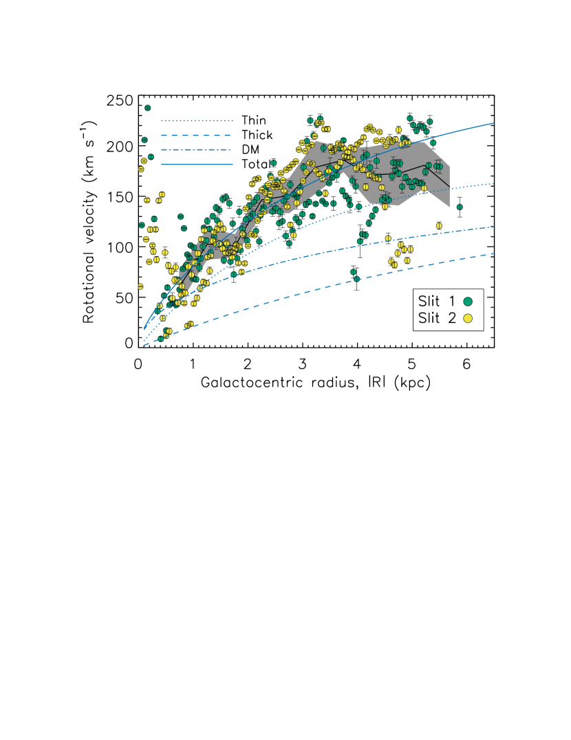
Figure 10.— The observed and modeled rotation curves of M83. The observed velocities from slits 1 (green points) and 2 (yellow points) are shown corrected for inclination and position angle ($v_{\phi}=(v_{obs}-v_{sys})/(\text{cos}(\phi)\text{sin}(i))$). For observations on the southwest side of the galaxy, the signs of $R$ and $v_{\phi}$ are changed to allow overplotting. The broad component is not included in this analysis. The black line and shaded region indicate the median and median absolute deviation of the observed rotation curve in bins of $\Delta R=0.5$ kpc, respectively. Significant scatter around the median is expected due to velocities in the $R$ and $z$ directions as well as spiral structure. Velocities within $|R|=1$ kpc are highly affected by the bar kinematics. The rotation curve of the modeled thin disk (dotted blue line), thick disk (dashed blue line), and dark matter halo (dot-dashed blue line) are overplotted, with the quadrature sum of these components shown as the solid blue line.

Table 3M83 Mass Model

Parameter	Value	Reference
$\sigma_{z,t}(0)$	73  km s-1	(1)
$\rho_{0,t}$	$5\times 10^{8}\mbox{\,$M_{\odot}$}\text{kpc}^{-3}$	(1)
$h_{z,t}$	0.4 kpc	(1)
$h_{R,t}$	4 kpc	(1)
$\sigma_{z,th}(0)$	40  km s-1	(1)
$\rho_{0,th}$	$2\times 10^{7}\mbox{\,$M_{\odot}$}\text{kpc}^{-3}$	(1)
$h_{z,th}$	1.2 kpc	(1)
$h_{R,th}$	10 kpc	(1)
$a_{DM}$	20 kpc	(2)
$\rho_{0,DM}$	$6\times 10^{6}\mbox{\,$M_{\odot}$}\text{kpc}^{-3}$	(2)

Appendix C A Dynamical Equilibrium Model: Implications for $\sigma(z)$

Here, we consider a dynamical equilibrium model for the eDIG layer in M83 in which $\sigma$ is allowed to vary with $z$. To solve for the $\sigma(z)$ that satisfies the observed rotational velocity lag, $\frac{\partial v_{\phi}}{\partial z}$, we take partial derivatives of Equations (6) and (7) with respect to $R$ and $z$, respectively. We subtract one from the other, assuming that $\sigma$ varies much more rapidly in $z$ than in $R$ ($\frac{\partial\sigma^{-2}}{\partial R}$ = 0). This yields:

$$0=\frac{\partial\sigma^{-2}}{\partial z}\bigg{(}\frac{\partial\Phi}{\partial R}-\frac{v_{\phi}^{2}}{R}\bigg{)}-\frac{\sigma^{-2}}{R}\frac{\partial v_{\phi}^{2}}{\partial z}.$$ (18)

Integrating Equation (18) with respect to $z$, we find:

$$\sigma(z_{2})=\sigma(z_{1})\bigg{[}\text{exp}\bigg{\{}\int_{z_{1}}^{z_{2}}\frac{1}{R}\frac{\partial v_{\phi}^{2}}{\partial z^{\prime}}\bigg{(}\frac{\partial\Phi}{\partial R}-\frac{v_{\phi}^{2}}{R}\bigg{)}^{-1}\text{d}z^{\prime}\bigg{\}}\bigg{]}^{-1/2}.$$ (19)

We evaluate this expression as follows. We assume that the gaseous disk is co-rotating within the HI thin disk scale height, $z<h_{HI}=0.1\text{ kpc}$. At $z=h_{HI}$, we set $v_{\phi}(h_{HI})=\sqrt{R\frac{\partial\Phi(h_{HI})}{\partial R}}-\epsilon$. At $z>h_{HI}$, we impose a rotational velocity gradient such that $v_{\phi}(z)=v_{\phi}(h_{HI})+\frac{\partial v_{\phi}}{\partial z}z$. We do not allow the gas to counter-rotate.

The use of an $\epsilon$ term is necessary to avoid the divergence of the integral in Equation (19) at $z=h_{HI}$, and follows physically from the reduction of the rotational velocity with respect to the circular velocity due to an outward pressure gradient. A preferred value of $\epsilon$ is found by setting $\frac{\partial P}{\partial R}=\frac{\sigma^{2}\rho}{h_{R,t}}$ in Equation (7), where $h_{R,t}$ is the thin disk radial scale length. At $R=h_{R,t}$, $\epsilon=30$  km s^-1; since $\sigma(z)$ is highly sensitive to $\epsilon$, and we consider both a small ($\epsilon=3$  km s^-1) and a preferred ($\epsilon=30$  km s^-1) value.

The observations favor a fairly steep rotational velocity gradient. The median observed difference in radial velocity between the narrow and the broad component is $\Delta v=-24$  km s^-1in projection, or $\Delta v=-70$  km s^-1corrected for inclination. If we are detecting gas at the scale height, $h_{z}\geq 1$ kpc, then the rotational velocity lag is at least a few tens of  km s^-1kpc^-1. If, as expected, we are detecting the densest eDIG closest to the disk, $z<h_{z}$, then the rotational velocity lag may be even steeper.

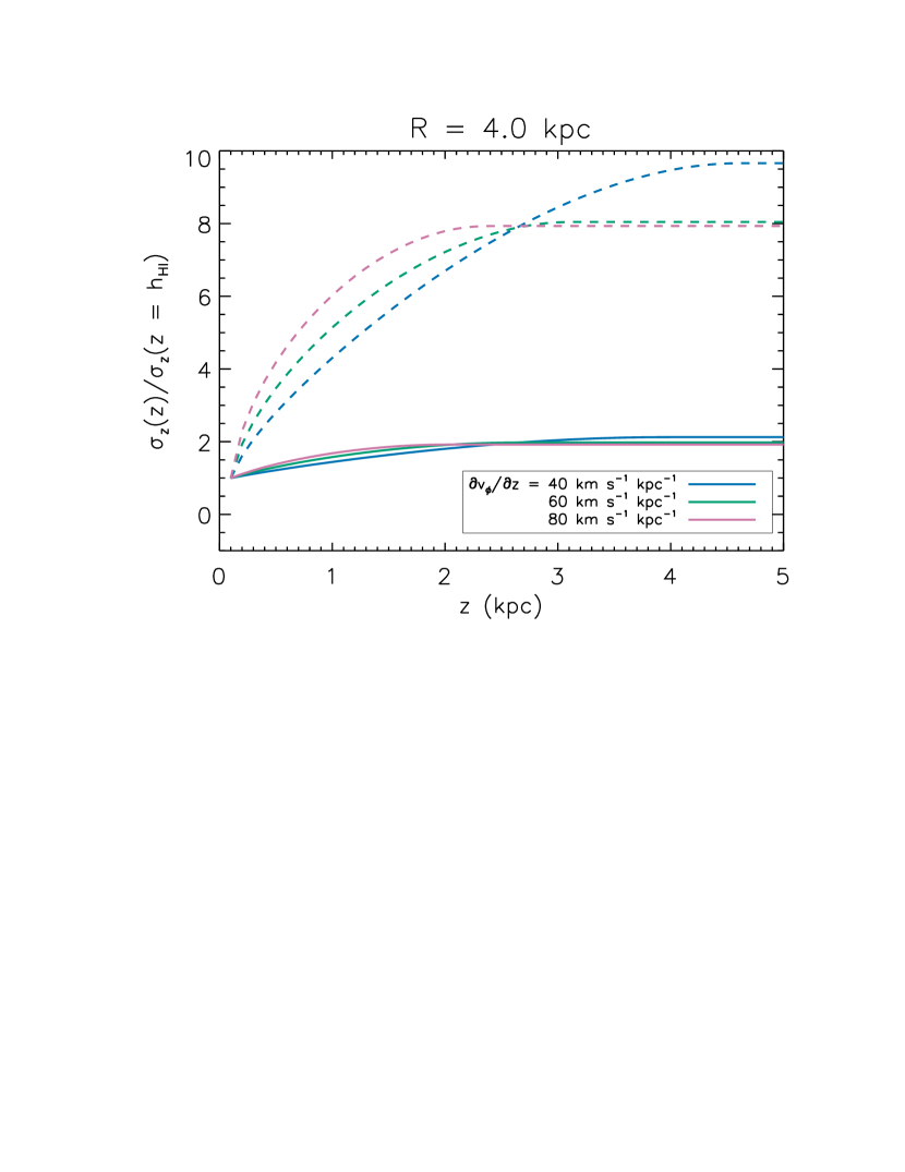
Figure 11.— $\sigma(z)$ required to produce a range of rotational velocity gradients in dynamical equilibrium for $\epsilon=\sqrt{R\frac{\partial\Phi(h_{HI})}{\partial R}}-v_{\phi}(h_{HI})=3$  km s^-1(dashed lines) and $\epsilon=30$  km s^-1(solid lines). For the preferred (larger) $\epsilon$, $\sigma$ must increase by a factor of two within $z=5$ kpc. However, for the smaller $\epsilon$, $\sigma$ must increase by an order of magnitude, posing a problem for the energetics of the system. The result is shown at $R=4$ kpc, but similar results are found at other galactocentric radii. Without knowledge of $\epsilon$, this class of models is highly unconstrained, and we regard the solutions as contrived.

In Figure 11, we show the $\sigma(z)$ required to produce a range of $\frac{\partial v_{\phi}}{\partial z}$ in dynamical equilibrium at $R=4$ kpc. Similar results are found at other galactocentric radii. Without knowledge of $\epsilon$, this class of models is highly unconstrained. For $\epsilon=30$  km s^-1(solid lines), an increase in $\sigma$ by a factor of two is required to produce a rotational velocity gradient of at least a few tens of  km s^-1kpc^-1. For $\epsilon=3$  km s^-1(dashed lines), an increase in $\sigma$ by an order of magnitude is required instead. Taken at face value, this suggests a velocity dispersion of several hundred  km s^-1at large $z$, consistent with the sound speed in a $T=10^{7}$ K gas. As this is an order of magnitude hotter than expected for the hot halo gas, small values of $\epsilon$ present a problem for the energetics of the system.

Thus, simultaneously satisfying the observed velocity dispersion and rotational velocity gradient while keeping the energy requirements reasonable requires fine-tuning of the model. We regard this model as contrived, but present it for completeness. This result emphasizes the importance of deep spectroscopic observations of edge-on eDIG layers, in which $\sigma(z)$ and $\frac{\partial v_{\phi}}{\partial z}$ can be quantified and this class of model can be constrained.

References

- Barnabè et al. (2006) Barnabè, M., Ciotti, L., Fraternali, F., & Sancisi, R. 2006, A&A, 446, 61
- Bizyaev et al. (2017) Bizyaev, D., Walterbos, R. A. M., Yoachim, P., et al. 2017, ApJ, 839, 87
- Boettcher et al. (2016) Boettcher, E., Zweibel, E. G., Gallagher, III, J. S., & Benjamin, R. A. 2016, ApJ, 832, 118
- Bregman (1980) Bregman, J. N. 1980, ApJ, 236, 577
- Bresolin et al. (2005) Bresolin, F., Schaerer, D., González Delgado, R. M., & Stasińska, G. 2005, A&A, 441, 981
- Buckley et al. (2006) Buckley, D. A. H., Swart, G. P., & Meiring, J. G. 2006, in Proc. SPIE, Vol. 6267, Society of Photo-Optical Instrumentation Engineers (SPIE) Conference Series, 62670Z
- Burgh et al. (2003) Burgh, E. B., Nordsieck, K. H., Kobulnicky, H. A., et al. 2003, in Proc. SPIE, Vol. 4841, Instrument Design and Performance for Optical/Infrared Ground-based Telescopes, ed. M. Iye & A. F. M. Moorwood, 1463–1471
- Calzetti et al. (2004) Calzetti, D., Harris, J., Gallagher, III, J. S., et al. 2004, AJ, 127, 1405
- Collins et al. (2002) Collins, J. A., Benjamin, R. A., & Rand, R. J. 2002, ApJ, 578, 98
- Collins & Rand (2001) Collins, J. A., & Rand, R. J. 2001, ApJ, 551, 57
- Crawford et al. (2010) Crawford, S. M., Still, M., Schellart, P., et al. 2010, in Proc. SPIE, Vol. 7737, Observatory Operations: Strategies, Processes, and Systems III, 773725
- Cuddeford (1993) Cuddeford, P. 1993, MNRAS, 262, 1076
- de Vaucouleurs et al. (1991) de Vaucouleurs, G., de Vaucouleurs, A., Corwin, Jr., H. G., et al. 1991, Third Reference Catalogue of Bright Galaxies. Volume I: Explanations and references. Volume II: Data for galaxies between 0h and 12h. Volume III: Data for galaxies between 12h and 24h. (New York, NY: Springer)
- Dettmar (1990) Dettmar, R.-J. 1990, A&A, 232, L15
- Draine (2011) Draine, B. T. 2011, Physics of the Interstellar and Intergalactic Medium (Princeton, NJ: Princeton University Press)
- Fraternali & Binney (2006) Fraternali, F., & Binney, J. J. 2006, MNRAS, 366, 449
- Fraternali et al. (2004) Fraternali, F., Oosterloo, T., & Sancisi, R. 2004, A&A, 424, 485
- Fraternali et al. (2002) Fraternali, F., van Moorsel, G., Sancisi, R., & Oosterloo, T. 2002, AJ, 123, 3124
- Haffner et al. (1999) Haffner, L. M., Reynolds, R. J., & Tufte, S. L. 1999, ApJ, 523, 223
- Haffner et al. (2003) Haffner, L. M., Reynolds, R. J., Tufte, S. L., et al. 2003, ApJS, 149, 405
- Heald et al. (2016) Heald, G., de Blok, W. J. G., Lucero, D., et al. 2016, MNRAS, 462, 1238
- Heald et al. (2006a) Heald, G. H., Rand, R. J., Benjamin, R. A., & Bershady, M. A. 2006a, ApJ, 647, 1018
- Heald et al. (2007) —. 2007, ApJ, 663, 933
- Heald et al. (2006b) Heald, G. H., Rand, R. J., Benjamin, R. A., Collins, J. A., & Bland-Hawthorn, J. 2006b, ApJ, 636, 181
- Herrmann & Ciardullo (2009) Herrmann, K. A., & Ciardullo, R. 2009, ApJ, 705, 1686
- Hong et al. (2011) Hong, S., Calzetti, D., Dopita, M. A., et al. 2011, ApJ, 731, 45
- Huchtmeier & Bohnenstengel (1981) Huchtmeier, W. K., & Bohnenstengel, H.-D. 1981, A&A, 100, 72
- Ivezić et al. (2014) Ivezić, Ž., Connelly, A. J., VanderPlas, J. T., & Gray, A. 2014, Statistics, Data Mining, and Machine Learningin Astronomy (Princeton, NJ: Princeton University Press)
- Jarrett et al. (2013) Jarrett, T. H., Masci, F., Tsai, C. W., et al. 2013, AJ, 145, 6
- Karachentsev et al. (2007) Karachentsev, I. D., Tully, R. B., Dolphin, A., et al. 2007, AJ, 133, 504
- Kobulnicky et al. (2003) Kobulnicky, H. A., Nordsieck, K. H., Burgh, E. B., et al. 2003, in Proc. SPIE, Vol. 4841, Instrument Design and Performance for Optical/Infrared Ground-based Telescopes, ed. M. Iye & A. F. M. Moorwood, 1634–1644
- Lehnert & Heckman (1995) Lehnert, M. D., & Heckman, T. M. 1995, ApJS, 97, 89
- Long et al. (2014) Long, K. S., Kuntz, K. D., Blair, W. P., et al. 2014, ApJS, 212, 21
- Madsen et al. (2006) Madsen, G. J., Reynolds, R. J., & Haffner, L. M. 2006, ApJ, 652, 401
- Oosterloo et al. (2007) Oosterloo, T., Fraternali, F., & Sancisi, R. 2007, AJ, 134, 1019
- Osterbrock & Ferland (2006) Osterbrock, D. E., & Ferland, G. J. 2006, Astrophysics of gaseous nebulae and active galactic nuclei (Sausalito, CA: University Science Books)
- Otte et al. (2002) Otte, B., Gallagher, III, J. S., & Reynolds, R. J. 2002, ApJ, 572, 823
- Park et al. (2001) Park, O.-K., Kalnajs, A., Freeman, K. C., et al. 2001, in Astronomical Society of the Pacific Conference Series, Vol. 230, Galaxy Disks and Disk Galaxies, ed. J. G. Funes & E. M. Corsini, 109–110
- Rand (1997) Rand, R. J. 1997, ApJ, 474, 129
- Rand (1998) —. 1998, ApJ, 501, 137
- Reynolds et al. (1998) Reynolds, R. J., Hausen, N. R., Tufte, S. L., & Haffner, L. M. 1998, ApJ, 494, L99
- Rossa & Dettmar (2003) Rossa, J., & Dettmar, R.-J. 2003, A&A, 406, 493
- Sembach et al. (2000) Sembach, K. R., Howk, J. C., Ryans, R. S. I., & Keenan, F. P. 2000, ApJ, 528, 310
- Shapiro & Field (1976) Shapiro, P. R., & Field, G. B. 1976, ApJ, 205, 762
- Shore (1992) Shore, S. N. 1992, An introduction to astrophysical hydrodynamics (San Diego: Academic Press)
- Soria & Wu (2002) Soria, R., & Wu, K. 2002, A&A, 384, 99
- Soria & Wu (2003) —. 2003, A&A, 410, 53
- van Dokkum (2001) van Dokkum, P. G. 2001, PASP, 113, 1420