Identification of Majorana Modes in Interacting Systems by Local Integrals of Motion.

Abstract

Recently, there has been substantial progress in methods of identifying local integrals of motion in interacting integrable models or in systems with many-body localization. We show that one of these approaches can be utilized for constructing local, conserved, Majorana fermions in systems with an arbitrary many-body interaction. As a test case, we first investigate a non-interacting Kitaev model and demonstrate that this approach perfectly reproduces the standard results. Then, we discuss how the many-body interactions influence the spatial structure and the lifetime of the Majorana modes. Finally, we determine the regime for which the information stored in the Majorana correlators is also retained for arbitrarily long times at high temperatures. We show that it is included in the regime with topologically protected soft Majorana modes, but in some cases is significantly smaller.

Introduction.—Recently, a lot of hope has been pinned on Majorana zero modes as building blocks of a quantum computer Aasen et al. (2016); Sarma et al. (2015); Karzig et al. (2017); Plugge et al. (2016); Akhmerov (2010). One of the systems where these modes were proposed and observed is a semiconductor nanowire with a spin-orbit interaction coupled to an $s$-wave superconductor Lutchyn et al. (2010); Oreg et al. (2010); Franz (2013); Mourik et al. (2012); Nadj-Perge et al. (2014); Pawlak et al. (2016); Ruby et al. (2015). It is known that, in low-dimensional systems, Coulomb interactions are crucial and can drastically affect their properties Haldane (1981); Gangadharaiah et al. (2011); Manolescu et al. (2014); Vuik et al. (2016); Domínguez et al. (2017a). Interactions are also important for practical reasons: disorder is present in any semiconductor nanowire and the Majorana states are not completely immune against it Maśka et al. (2017); Lutchyn et al. (2011); Akhmerov et al. (2011). Moderate interactions may stabilize the Majorana states against such perturbations Domínguez et al. (2017b); Stoudenmire et al. (2011); Gergs et al. (2016); Hassler and Schuricht (2012).

Generally, a Majorana fermion is any fermionic operator $\Gamma$ that satisfies $\Gamma^{2}=1$. However, in order to perform topological quantum computing one needs stable, non-Abelian anions Nayak et al. (2008). They can be realized as localized Majorana zero modes (MZMs), whereby their stability follows from the commutation relation

$$\left[\hat{H},\,\Gamma\right]=0,$$ (1)

where $\hat{H}$ is the Hamiltonian. This equation together with the conservation of the fermion parity lead to a non-Abelian braiding for adiabatic exchanging of Majorana quasiparticles Clarke et al. (2011). Equation (1) can be fulfilled rigorously only in the thermodynamic limit, except for a fine-tuned symmetric point Kitaev (2001) where it also holds true for finite $L$. In general, $\left[\hat{H},\,\Gamma\right]\propto e^{-L/\xi}$, where $L$ is the system size and $\xi$ is correlation length Kells (2015). The nonzero value of the commutator means that, even in the absence of any external decoherence processes, the MZM will have a finite lifetime.

The question is how to find the topological order and Majorana modes in interacting systems. Several methods have been used to study MZMs in interacting nanowires Ng (2015); Su et al. (2016); Chan et al. (2015); Hofmann et al. (2016); Thomale et al. (2013), see Ref. Stoudenmire et al. (2011) for a review. A commonly tested necessary condition [which follows from Eq. (1)] concerns degeneracy of the ground states obtained for systems with odd and even numbers of fermions. A sufficient condition for the presence of topological order is more involved. It can be formulated based on the local unitary equivalence (LUE) between the ground states of the interacting system and of the noninteracting Kitaev chain in the topological phase Chen et al. (2011). In order to prove LUE, it is sufficient to show that one of the ground states can be continuously deformed to the other, whereby the spectral gap above the ground state must stay open along the entire path of deformation Fidkowski and Kitaev (2010); Katsura et al. (2015). But this is not equivalent to Eq. (1) and guarantees only the so-called soft mode, which is fully protected by topology only at temperatures well below the spectral gap. In other words, a soft MZM commutes with the Hamiltonian which is projected into a low-energy subspace Alicea and Fendley (2016). At higher temperatures, the information encoded in this mode can be lost after some time.

In this Letter, we propose a method that allows one to find Majorana operator $\Gamma$ that almost satisfies Eq. (1) within the entire Hilbert space. Our method finds the so-called strong MZM that is stable at arbitrary high temperatures Else et al. (2017); Goldstein and Chamon (2012); Kemp et al. (2017). Perturbative construction of almost strong MZMs has recently been reported in Ref. Kemp et al. (2017) for the Ising–like model with nearest- and (integrability-breaking) next-nearest-neighbor interactions. In contradistinction, our approach is general and can be applied for arbitrary Hamiltonians, in principle, also, for spinful fermions. To this end, we derive the optimal form of a local operator $\Gamma$ that guarantees the longest lifetime of the MZM. We determine the regime of existence of a strong MZM and show that it is smaller than the regime with soft modes, the latter being established from LUE.

The general method.—We consider the Hamiltonian $\hat{H}=\sum_{m}E_{m}|m\rangle\langle m|$ and assume that the relevant degrees of freedom can be expressed in terms of the standard fermionic operators $a_{j}$ and $a^{\dagger}_{j}$ or, equivalently, in terms of the Majorana fermions $\gamma_{2j}=a_{j}+a_{j}^{\dagger}$, $\gamma_{2j+1}=i(a_{j}^{\dagger}-a_{j})$. Here, $j$ includes all quantum numbers, e.g., the spin projection. We search for particular combinations of the Majorana operators $\Gamma=\sum_{i}\alpha_{i}\gamma_{i}$ with real coefficients $\alpha_{i}$ such that $\Gamma$ is conserved mul . We assume normalization $\sum_{i}\alpha_{i}^{2}=1$ when $\Gamma^{2}=1$. The conservation of $\Gamma$ can conveniently be studied by averaging this quantity over an infinite time window

$$\bar{\Gamma} = \lim_{\tau^{\prime}\rightarrow\infty}\frac{1}{\tau^{\prime}}\int_{0}^{\tau^{\prime}}{\mathrm{d}}te^{iHt}\Gamma e^{-iHt},$$ (2)

$$= \lim_{\tau\rightarrow\infty}\sum_{m,n}\theta\left(\frac{1}{\tau}-|E_{m}-E_{n}|\right)\langle n|\Gamma|m\rangle\;\;|n\rangle\langle m|.$$ (3)

If this mode is strictly conserved then $\bar{\Gamma}=\Gamma$. This, however, would require Eq. (1) to be satisfied, what may not be the case in finite systems. Therefore, we will usually search for an optimal choice of $\alpha_{i}$ when $\bar{\Gamma}$ is as close to $\Gamma$ as possible. In order to quantify the proximity of two operators we use the usual (Hilbert-Schmidt) inner product $\langle\hat{A}\hat{B}\rangle=\mathrm{Tr}(\hat{A}\hat{B})/\mathrm{Tr}(\hat{1})$. The optimal choice of coefficients $\alpha_{i}$ corresponds to a minimum of $\langle(\Gamma-\bar{\Gamma})^{2}\rangle=1-\langle\bar{\Gamma}^{2}\rangle$. The latter equality originates from the identity $\langle\Gamma\bar{\Gamma}\rangle=\langle\bar{\Gamma}\bar{\Gamma}\rangle$ (i.e., the time averaging is an orthogonal projection), as shown in the Supplemental Material sup . Consequently, the least decaying mode can be found from the optimization problem

$$\lambda=\max_{\{\alpha_{i}\}}\,\langle\bar{\Gamma}^{2}\rangle=\max_{\{\alpha_{i}\}}\,\langle\bar{\Gamma}\Gamma\rangle.$$ (4)

The physical meaning of $\lambda$ comes from the observation that the scalar product $\langle...\rangle$ formally represents thermal averaging carried out for infinite temperatures. Then, following Eq. (4), $\lambda$ is the asymptotic value of the longest living autocorrelation function $\langle\Gamma(t)\Gamma\rangle$. If $\lambda=1$, then $\Gamma$ is a strict integral of motion. i.e. a strong MZM Else et al. (2017); Fendley (2016); Alicea and Fendley (2016); Jermyn et al. (2014). For $0<\lambda<1$ the information stored in the correlator $\langle\Gamma(t)\Gamma\rangle$ is partially retained for arbitrarily long times (despite $\Gamma$ not being strictly conserved), while this information is completely lost when $\lambda=0$. The optimization problem can be further simplified

$$\lambda=\max_{\{\alpha_{i}\}}\sum_{ij}\alpha_{i}\langle\bar{\gamma}_{i}\bar{\gamma}_{j}\rangle\alpha_{j}.$$ (5)

It becomes a standard eigenproblem for the (positive semidefinite) matrix $\langle\bar{\gamma}_{i}\bar{\gamma}_{j}\rangle$. Namely, $\lambda$ is the largest eigenvalue of $\langle\bar{\gamma}_{i}\bar{\gamma}_{j}\rangle$, and $\alpha_{j}$ are components of the corresponding eigenvector. Essentially, all nonvanishing eigenvalues (whether degenerate or not) correspond to independent MZMs, whereby their independence follows from orthogonality of different eigenvectors and the identity $\langle\gamma_{i}\gamma_{j}\rangle=\delta_{ij}$.

The general idea behind this method is similar to another approach which has previously been used for identification of new integrals of motion in the Heisenberg model Mierzejewski et al. (2015a). The latter approach targets operators which are conserved and local. Here, we single out Majorana operators which are conserved and, at the same time, are local. The conservation follows from the time averaging, i.e., from the identity $[\hat{H},\bar{\Gamma}]=0$, whereas locality originates from the fact that $\Gamma$ is a linear combination of $\gamma_{i}$, each of them being supported on a single site only. Since we maximize the projection $\langle\bar{\Gamma}\Gamma\rangle$, the resulting operators retain the properties of both $\Gamma$ and $\bar{\Gamma}$; i.e., they are local, conserved MZMs. More formal discussion concerning MZMs (including their locality O’Brien and Wright ) can be found in the Supplemental Material sup .

When studying systems with fixed boundary conditions, it is utterly important, that the limit for the size of the system $L\rightarrow\infty$ precedes the limit for time $\tau\rightarrow\infty$, Rigol and Shastry (2008); Sirker et al. (2014). Since numerical calculations can be carried out for finite systems only, $\tau$ in Eq. (3) should be kept large but finite until the finite–size scaling is accomplished. All the discussed properties of the correlation functions also hold true for finite $\tau$ Mierzejewski et al. (2015b); Prelovšek et al. (2017), even though it is not the case for finite $\tau^{\prime}$ in Eq. (2).

Example.—As an example, we study a one–dimensional system of interacting, spinless fermions with hard-wall boundary conditions. The system is described by the Kitaev Hamiltonian Kitaev (2001) extended by the many body interactions

$$\hat{H} = -t_{0}\sum_{i=1}^{L-1}\left(a_{i+1}^{\dagger}a_{i}+\text{H.c.}\right)+\Delta\sum_{i=1}^{L-1}\left(a_{i+1}^{\dagger}a_{i}^{\dagger}+\text{H.c.}\right)$$ (6)

$$-\mu\sum_{i=1}^{L}\widetilde{n}_{i}+V\sum_{i=1}^{L-1}\widetilde{n}_{i}\widetilde{n}_{i+1}+W\sum_{i=1}^{L-1}\widetilde{n}_{i}\widetilde{n}_{i+2}.$$

Here, $t_{0}$ refers to hopping amplitude, $\mu$ is a chemical potential, $\Delta$ is the superconducting gap and $\widetilde{n}_{i}=a_{i}^{\dagger}a_{i}-\frac{1}{2}$. $V$ and $W$ are potentials of the first and second nearest-neighbor interactions. For simplicity, we use dimensionless units by putting $\hbar=1$ and $t_{0}$=$1$.

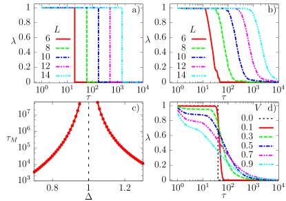
Figure 1: Results for systems without (a,c) and with (b,d) many-body interactions and $\mu=0$. (a), (b) and (d) The Majorana autocorrelation function $\lambda$ [see Eq. (4)] for: (a) $V=0,\Delta=0.5$; (b) $V=0.2,\Delta=0.5$; (d) $L=12,\Delta=0.3$. (c) Lifetime of MZMs for a finite noninteracting system of $L=10$ sites.

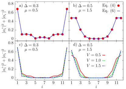
Figure 2: Spatial structure of MZMs, $\Gamma^{+}=\sum_{i}\alpha^{+}_{i}\gamma_{2i}$ and $\Gamma^{-}=\sum_{i}\alpha^{-}_{i}\gamma_{2i+1}$. a) and b) Rescaled local density of states at energy $E=0$ for noninteracting system [$V=0$ , Eq. (7)] (solid line) compared with solution of Eq. (5) (points). c) and d) Results for $V\neq 0$ from Eq. (5).

Test for noninteracting systems.—Numerical implementation of our approach consists of three consecutive steps: (i) exact diagonalization of the Hamiltonian (6); (ii) numerical construction of time–averaged Majorana operators $\bar{\gamma}_{i}$ as defined by Eq. (3) but for finite $\tau$; (iii) construction and diagonalization of the matrix $K_{ij}=\langle\bar{\gamma}_{i}\bar{\gamma}_{j}\rangle$. Because of the orthogonality relation $\langle\bar{\gamma}_{2i}\bar{\gamma}_{2j+1}\rangle=0$, one may separately study two cases $\Gamma^{+}=\sum_{i}\alpha^{+}_{i}\gamma_{2i}$ and $\Gamma^{-}=\sum_{i}\alpha^{-}_{i}\gamma_{2i+1}$, whereby, now, the index $i$ enumerates the lattice sites. In the rest of this work, we discuss the two most stable modes (one in each sector $\Gamma^{+}$ and $\Gamma^{-}$). All other eigenvalues of the matrix $K$ are much smaller and vanish in the thermodynamic limit (not shown). It remains in agreement with a common knowledge that the homogeneous chain described by the Hamiltonian (6) may host at most two MZMs exponentially localized at the boundaries Kitaev (2001); Kells (2015); Katsura et al. (2015) .

The complexity of our approach is independent of whether or not the many-body interactions are present: hence, the method can be tested by investigating a noninteracting system with $V=W=0$. Figiure 1a) shows $\tau$ dependence of $\lambda$ [see Eq. (4)] for the most stable MZM $\Gamma^{+}$. Results for $\Gamma^{-}$ are exactly the same. One may introduce the lifetime of the MZMs, $\tau_{M}$, corresponding to the vertical sections of curves shown in the latter plot. Figure 1c) shows that, for finite system, $\tau_{M}$ is finite as well, despite the absence of the many-body scattering. The only exception concerns $|\Delta|=1$ when $\tau_{M}\rightarrow\infty$ for arbitrary $L$. Otherwise, $\tau_{M}$ increases exponentially with $L$, as follows from the equal spacing of the vertical sections in Fig. 1a). The latter result clearly illustrates the importance of the correct order of limits: $\lim_{\tau\rightarrow\infty}\lim_{L\rightarrow\infty}\lambda=1$; i.e., the MZMs are strictly conserved in the thermodynamic limit, while $\lim_{L\rightarrow\infty}\lim_{\tau\rightarrow\infty}\lambda=0$. All the obtained results remain in agreement with the well established properties of the MZMs in a noninteracting case, see, e.g., Kells (2015).

We have also calculated the local density of states at zero energy for the noninteracting Hamiltonian

$$\rho_{i}(E=0)=-\frac{1}{\pi}{\rm Im}\,G_{ii}(E=0),\ \ \ G(E)=(E-\hat{H}+i\eta)^{-1},$$ (7)

where $\hat{H}$ is given by Eq. (6) but with $V=W=0$. In Figs. 2a) and 2b), rescaled $\rho_{i}(E=0)$ is compared with the spatial density of the Majorana fermions contributing to both Majorana modes, $|\alpha^{+}_{i}|^{2}+|\alpha^{-}_{i}|^{2}$. Perfect agreement between both methods illustrates accuracy of the approach derived in this work.

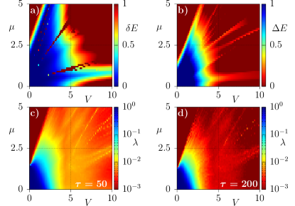
Figure 3: Results for $\Delta=1$. a) Degeneracy of the ground states. b) The spectral gap. c) and d) show the Majorana autocorrelation function $\lambda$ for various times $\tau$ and $L=12$. Note different color schemes in a) and b).

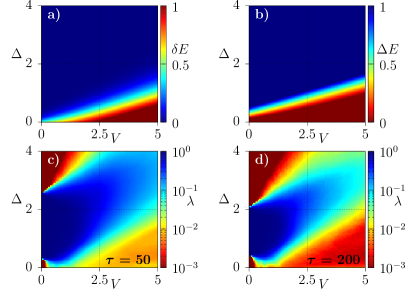
Figure 4: The same as in Fig. 3, but as a function of $V$ and $\Delta$ for $\mu=0$.

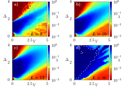
Figure 5: The autocorrelation function $\lambda$ as a function of $V$ and $\Delta$ for $\tau=100$ and various system sizes $L$. Contour in d) marks $\lambda=0.8$.

Systems with many-body interactions.—All results in the main text will be shown for $W=V/2$, whereas the commonly studied case $W=0$ (which contains some peculiar features) is discussed in the Supplemental Material sup . Results in Figs. 1b) and 1d) show the most stable Majorana autocorrelation function [Eq. (4)] in the presence of weak to moderate interactions. Similar to the noninteracting case [Fig. 1a)], the position of the steep sections of $\lambda(\tau)$ increases exponentially with the system size indicating that $\lim_{\tau\rightarrow\infty}\lim_{L\rightarrow\infty}\lambda\simeq 1$ but, in contrast to noninteracting systems, $\lambda<1$. In the Supplemental Material sup , we show that the latter inequality seems to be generic for systems with many-body interactions. It implies that the strictly local operator $\Gamma$ is not a strict integral of motion. Our approach singles out $\Gamma$ which contains the largest possible conserved part represented by $\lim_{\tau\rightarrow\infty}\bar{\Gamma}$.

For finite systems, the many-body interactions may extend the time scale in which the correlator $\langle\Gamma(t)\Gamma\rangle$ is large. Interestingly, this extension can exceed 1 order of magnitude, as shown in Fig. 1d). Figures 2c) and 2d) explain the origin of this extension. They show how the many-body interactions modify the spatial structure of the MZMs. There are two modes which vanish exponentially outside of the edges of the system. Note that this property is not built into our algorithm but appears as a result which doesn’t need to hold true for other geometry of the system. Despite the exponential decay, these two modes still do overlap and this overlap is responsible for a finite-lifetime of the MZMs in a noninteracting system with $L<\infty$. Then, the many-body interactions push these modes further towards the edges of the system [see Figs. 2c) and 2d)], reducing the overlap between them and, in this way, increasing their lifetime. This mechanism holds true as long as the interactions are not too strong, when the MZMs eventually disappear.

Next, we compare our results for strong MZMs with the presence of the topological order. We check the degeneracy of the ground state (necessary condition) as well as LUE to the topological regime in the noninteracting Kitaev model (sufficient condition). To this end, we study chains of $L=8,10,...,20$ and find the two lowest energies in the subspaces with odd and even particle numbers, denoted, respectively, as $E_{0,o}(L)$, $E_{1,o}(L)$ and $E_{0,e}(L)$, $E_{1,e}(L)$. We introduce the measure of the ground–state degeneracy $\delta E(L)=E_{0,o}(L)-E_{0,e}(L)$ and two spectral gaps, $\Delta E_{o(e)}(L)=E_{1,o(e)}(L)-E_{0,o(e)}(L)$. Typically, the gaps between the low–energy levels decay algebraically with $L$; hence, we carry out linearly in $1/L$ extrapolations of $\Delta E_{o(e)}(L)$. However, $\delta E(L)$ should decay exponentially in the topological regime; thus, we use the fitting function $\delta E(L)=A\exp(-BL)+\delta E(\infty)$. These extrapolations break down when $V$ and $\mu$ are large sup , what shows up as large errors for the extrapolated quantities, $\sigma_{\delta E}$ and $\sigma_{\Delta E}$. We identify the degenerate ground states as a regime where both $|\delta E(\infty)|$ and $\sigma_{\delta E}$ are small, defining $\delta E\equiv|\delta E(\infty)|+\sigma_{\delta E}\ll 1$ as the lower bound on the degenerate region. The LUE implies that the gap $\min\{\Delta E_{o}(\infty),\Delta E_{e}(\infty)\}$ doesn’t vanish along a path that reaches the topological regime for $V=0$, while $\sigma_{\Delta E}$ remains small. Then, we define the lower bound on the corresponding region by $\Delta E\equiv\min\{\Delta E_{o}(\infty),\Delta E_{e}(\infty)\}-\sigma_{\Delta E}>0$. Results for $\delta E$ and $\Delta E$ are shown in Figs. 3a), 4a) and 3b), 4b), respectively. The actual topological region may be larger than it follows from lower bounds shown in Figs. 3b) and 4b).

Results in Figs. 3c) and 3d) show that the strong MZMs, indeed, exist for very long times ($\tau>200$) not only in the ground state but, essentially, in the entire energy spectrum. We also confirm that a moderate many-body interaction extends the range of $\mu$ where soft and strong MZMs are present Stoudenmire et al. (2011).

In Fig. 4, we show similar results but for $\mu=0$ and various magnitudes of the superconducting gap $\Delta$. In this case an exact solution is known but only for $\Delta=1$ and $W=0$ Katsura et al. (2015); Miao et al. (2017). For large $\tau$ and $\Delta\gg 1$, the strong MZMs seem to be absent even for very weak many-body interaction. However, it is a finite-size effect that, again, shows how important is the correct order of limits for time and the system size. Therefore, in Fig. 5 we set $\tau=100$ and show the Majorana autocorrelation function for various values of $L$ together with results extrapolated to $L\rightarrow\infty$. The details of extrapolation and results for $\lim_{\tau\rightarrow\infty}\lim_{L\rightarrow\infty}\lambda(\tau)$ are shown in the Supplemental material sup . The regime with $\lambda>0$ covers roughly the entire topological regime determined via LUE to the single-particle Kitaev model [compare Figs. 4b) and 5d)]. However, $\lambda$ gradually decreases with increasing interactions, and a strong MZM with large $\lambda$ exists within a much smaller regime, as shown e.g., by the contour in Fig. 5d).

Conclusions.—We have proposed an approach for finding local (strong or almost strong) MZMs which can be implemented for an arbitrary many-body interaction. We have found that even at elevated temperatures, the lifetime of these modes is long enough so that they may be used effectively to store the information. The regime where the strong MZMs exist (as quantified by large $\lambda$ in our approach) is included, but is smaller than the regime which is unitarily equivalent to the topological regime in the single-particle Kitaev model. It means that not all topological states are equally protected to be useful in, e.q., quantum computing. At finite temperatures, the systems with weak many-body interactions are preferable; however, these interactions may still be significant, when compared to other energy scales in the system. Our results also suggest that in systems with many-body interactions the strictly local Majorana operators are not strict integrals of motion, however, their autocorrelation function remains large for arbitrarily long times.

This work is supported by the National Science Centre, Poland via Projects No. 2016/23/B/ST3/00647 (A.W. and M.M.) and No. DEC–2013/11/B/ST3/00824 (M.M.M.).

Supplemental Material for:
Majorana modes in interacting systems identified by searching for local integrals of motion Andrzej WięckowskiMaciej M. Maśka Marcin Mierzejewski

Part I Supplemental Material

In the Supplemental Material we show that the Majorana fermions singled out by our approach are indeed the edge strong zero modes. Further on, we discuss results for a system where the many–body interactions are restricted to the neighboring lattice sites only. Finally, we present the details of the finite–size scaling.

I Majorana edge zero mode

In this section, we closely follow the formal concept of strong edge zero mode described in Ref. Kemp et al. (2017); Else et al. (2017) and also in Goldstein and Chamon (2012). Such mode is an operator that maps an eigenstate in one symmetry sector to a state in another sector with the same energy up to finite-size corrections. Here, the term ”strong” means, that this mapping holds true for all eigenstates of Hamiltonian. As clearly explained in Ref. Kemp et al. (2017), it is a stronger condition than necessary for a topological order. Interestingly, the strong character of the Majorana zero modes has been recognized already in the pioneer paper by Kitaev Kitaev (2001). Below we demonstrate that for $\lambda=1$ [see Eq. (4) in the main text] the Majorana operator, $\Gamma=\sum_{i}\alpha_{i}\gamma_{i}$, is indeed a strong zero mode.

Using the commutation relations $\{\gamma_{i},\gamma_{j}\}=2\delta_{ij}$ one finds

$$\Gamma^{2}=\frac{1}{2}\sum_{ij}\alpha_{i}\alpha_{j}\{\gamma_{i},\gamma_{j}\}=\sum_{i}\alpha^{2}_{i}=1.$$ (S1)

We formally rewrite $\Gamma$ as well as $\bar{\Gamma}$ [see Eq. (2) in the main text] in the basis of the eigenstates of Hamiltonian

$$\Gamma = \sum_{m,n}\langle n|\Gamma|m\rangle\;\;|n\rangle\langle m|,$$ (S2)

$$\bar{\Gamma} = \sum_{m,n:E_{m}=E_{n}}\langle n|\Gamma|m\rangle\;\;|n\rangle\langle m|.$$ (S3)

$\bar{\Gamma}$ is strictly conserved, since it commutes with Hamiltonian,

$$[\bar{\Gamma},\hat{H}]=\sum_{m,n:E_{m}=E_{n}}(E_{m}-E_{n})\langle n|\Gamma|m\rangle\;\;|n\rangle\langle m|=0.$$ (S4)

In the main text we have shown that the condition $\lambda=1$ it equivalent to $\Gamma=\bar{\Gamma}$, hence for $\lambda=1$ one obtains also $\bar{\Gamma}^{2}=1$. Then, we see that

$$1=\langle n|\bar{\Gamma}^{2}|n\rangle=\sum_{m:E_{m}=E_{n}}|\langle n|\Gamma|m\rangle|^{2},$$ (S5)

holds true for arbitrary eigenstate $|n\rangle$. It is evident that the matrix elements $\langle n|\Gamma|m\rangle$ are nonzero only for states with opposite parity of the particle number. Assuming that the energy spectrum is at most doubly degenerate, we see that for each state $|m\rangle$ in one symmetry sector (e.g. with even number of electrons) there exists a state $|n\rangle$ in the other sector (e.g. with odd number of electrons) such that $E_{m}=E_{n}$. Using Eqs. (S2) and (S5) we obtain

$$\Gamma|m\rangle=\exp(i\phi_{n})|n\rangle,$$ (S6)

hence $\Gamma$ is indeed a strong zero mode.

Equation (S3) might suggest that numerical diagonalization of the Hamiltonian is sufficient to single out the Majorana strong zero modes. The only problem seems to be sorting the energies and finding the matching pairs of states $|n\rangle$ and $|m\rangle$ in different symmetry sectors but with equal energies. However, numerical diagonalization can be carried out for finite systems only when the energies of states with opposite parities differ by a finite-size corrections. Due to these corrections, one would have to find the pairs of states such that the difference of their energies vanishes in the thermodynamic limit, $L\rightarrow\infty$. Implementation of such numerical procedure is highly nontrivial, especially that the typical distance between the consecutive energy levels decays exponentially with $L$ for arbitrary extensive Hamiltonian, i.e., independently of the presence of the Majorana modes. In our approach the problem of the finite size corrections to the energy levels is resolved simply by allowing for finite $\tau$ in Eq. (2) in the main text. The correct order of limits $\lim_{\tau\rightarrow\infty}\lim_{L\rightarrow\infty}\lambda$ simply means that the strict degeneracy exists only in the thermodynamic limit. Even if the problem of not perfectly degenerate states could be resolved by some other method, then one needs to carry out an independent test whether the Majorana mode, as given by Eq. (S3), is a local operator with support at the edges of the system.

In our approach the largest eigenvalue $\lambda$ obtained from Eq. (4) in the main text allows to single out the Majorana strong zero mode $\Gamma=\sum_{i}\alpha_{i}\gamma_{i}$. As demonstrated in Fig. 2 in the main text, the coefficients $\alpha_{i}$ decay outside of regions located at the edges of the chain, hence $\Gamma$ is also the edge mode. It is important to stress that $\alpha_{i}$ and $\lambda$ are determined by a single eigenproblem. Consequently, the presence and properties of strong zero modes in the many-body Hamiltonian are fully specified by this eigenproblem. We are not aware of any other numerical algorithm, which allows to single out strong edge zero modes in arbitrary Hamiltonian with many-body interactions.

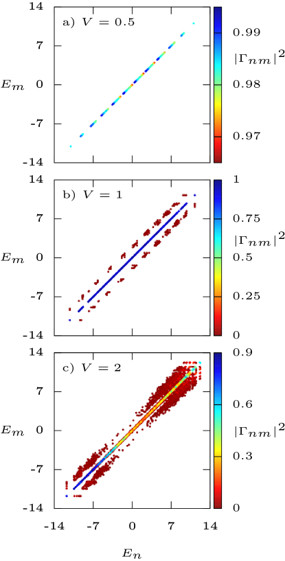
Figure S1: Squared matrix elements of the Majorana mode $|\Gamma_{nm}|^{2}=|\langle m|\Gamma|n\rangle|^{2}$ for $L=12$ and $W=V/2$. Panels a,b and c show results for $V=0.5$, $V=1$ and $V=2$, respectively. For such system we obtain at $\tau=10^{2}$, respectively, $\lambda\simeq 0.98$, 0.92 and 0.23. Note that each panel has a separate false color scheme.

II Almost conserved Majorana modes

In this section we discuss the physical meaning of the Majorana fermions for $0<\lambda<1$. Using Eq. (3) in the main text, one obtains

$$\langle\Gamma\Gamma\rangle = \frac{1}{Z}\sum_{n,m}|\langle n|\Gamma|m\rangle|^{2}=1,$$ (S7)

$$\langle\bar{\Gamma}\bar{\Gamma}\rangle = \frac{1}{Z}\sum_{n,m:E_{m}=E_{n}}|\langle n|\Gamma|m\rangle|^{2}=\lambda.$$ (S8)

where $Z=\sum_{n}1$ is the dimension of the Hilbert space. For $\lambda<1$, $\Gamma$ remains a local operator (e.g., the edge mode), since it is defined as a linear combination of the local Majorana operators $\gamma_{i}$. However, it is not strictly conserved any more. Using Eqs. (S7) and (S8) one finds for $\lambda<1$ that there are nonvanishing matrix elements $\langle n|\Gamma|m\rangle$ also for states with different energies $E_{m}\neq E_{n}$. Therefore, for $\lambda<1$ the strong character of the Majorana mode is lost. Then, it is instructive to decompose the Majorana operator in the following way

$$\Gamma=\bar{\Gamma}+\bar{\Gamma}^{\perp},$$ (S9)

where $\bar{\Gamma}$ is given by Eq. (S3). It represents the conserved part (zero mode) of the Majorana operator, $[\bar{\Gamma},H]=0$. The remaining part

$$\bar{\Gamma}^{\perp}=\sum_{m,n:E_{m}\neq E_{n}}\langle n|\Gamma|m\rangle\;\;|n\rangle\langle m|.$$ (S10)

is orthogonal to $\bar{\Gamma}$, $\langle\bar{\Gamma}\bar{\Gamma}^{\perp}\rangle=0$. Due to this orthogonality it is easy to find the (squared) norms of all operators:

$$||\Gamma||^{2} = \langle\Gamma\Gamma\rangle=1,$$ (S11)

$$||\bar{\Gamma}||^{2} = \langle\bar{\Gamma}\bar{\Gamma}\rangle=\lambda,$$ (S12)

$$||\bar{\Gamma}^{\perp}||^{2} = \langle\Gamma\Gamma\rangle-\langle\bar{\Gamma}\bar{\Gamma}\rangle=1-\lambda.$$ (S13)

To conclude, our approach finds the Majorana fermions with the largest $\lambda$. It singles out the Majorana strong zero-mode if such mode exists ($\lambda=1$). Otherwise ($\lambda<1$), it finds the Majorana mode with the largest conserved part, $\bar{\Gamma}$.

Figure S1 shows the matrix elements of such Majorana mode $\Gamma_{mn}=\langle m|\Gamma|n\rangle$ as a function of energies $E_{m}$ and $E_{n}$. Fig. S1a shows results for $L=12,V=0.5$ and $W=V/2$. For such parameters one obtains $\lambda\simeq 0.98$ for $\tau=10^{2}$ hence $\Gamma$ is (almost) a strong Majorana mode. In agreement with Eq. (S6), for each eigenstate $|n\rangle$ there exists a single state $|m\rangle$ with opposite parity such that $|\Gamma_{mn}|\simeq 1$ and $E_{m}\simeq E_{n}$. The middle panel shows results for the same system but with $V=1$ when $\lambda\simeq 0.92$ for $\tau=10^{2}$. Now, $\Gamma$ is not a strong zero mode any more. It contains a significant conserved part (zero mode), $\bar{\Gamma}$, represented by points along the diagonal and much smaller not conserved part, $\bar{\Gamma}^{\perp}$, represented by the off–diagonal elements. $\lambda$ is the ratio of contributions coming from the diagonal points [see Eq. (S8)] to the total contribution coming from all the points [see Eq. (S7)]. Finally, for even stronger interaction, $V=2$, we obtain $\lambda\simeq 0.23$ at $\tau=10^{2}$ and the corresponding matrix elements are shown in Fig. S1c. The conserved part is diminished mostly in the middle of the spectrum, but it still remains large at the bottom of the spectrum, what is relevant for the low–temperature regime. The Hilbert-Schmidt inner product $\langle...\rangle$ may be modified in such a way that it becomes relevant for finite temperatures, e.g. see Ref. Mierzejewski et al. (2015b). We have numerically studied selected cases also for $k_{B}T=10$ and found that the liftetime of the MZMs is slightly larger than at $T\rightarrow\infty$ (not shown). Obviously, very low but nonzero temperatures are not accessible due to huge finite–size effects.

III Results for a system with nearest neighbor interaction

Numerical results presented in the main text have been obtained for repulsive interaction between the first ($V$) and the second nearest neighbors ($W$). Here, we discuss the same quantities but for the commonly studied case with $W=0$ which, however, contains some peculiar features.

We start with the difference of the ground state energies $\delta E(L)$, obtained for systems with odd and even number of fermions. Vanishing of $\delta E$ in the thermodynamic limit is necessary for the onset of soft Majorana modes. $\delta E(L)$ obtained for $L=8$ is shown in Figs. S2a and S2b for $W=0$ and $W=V/2$, respectively. The former figure accurately reproduces results presented in Ref. Ng (2015). Here one may identify two regions where $\delta E(L)$ is small: (1) small 2D area around $V=0,\,\mu=0$ and (2) a number of narrow stripes that extend from region (1) to large–$V$ and large–$\mu$. While the internal structure of region (2) is hardly visible for $W=0$, it becomes very clear for $W=V/2$, as shown in Fig. S2b. It is composed of straight lines and their total number exactly equals the size of the system, whereby $L/2$ lines are explicitly visible in the figures, while remaining $L/2$ lines exist for $\mu<0$. The physical origin of these lines is explained in Figs. S2c and S2d where we show average particle number in the ground state, $\langle N\rangle$. We also mark the parameters for which $\delta E(L)$ is small. One can see that lines separate regimes where the ground state occupation is close to consecutive integers $0,1,\ldots,L$. In the adjoining regimes, these integers have opposite parity, hence the borderline between these regimes corresponds to degenerate ground states obtained in sectors with odd and even particle numbers. However, such lines exist independently of the pairing term, i.e., also in topologically trivial phases, and are thus unrelated to the local Majorana modes. The presence of the latter lines explains also why the finite–size scaling for $\delta E(L)$ breaks down in this regime. Since the number and positions of these lines change with $L$, $\delta E(L)$ may be non–monotonous functions of $L$. The same problem shows up also in the finite–size scaling of the spectral gaps $\Delta E_{o}(L)$ and $\Delta E_{e}(L)$.

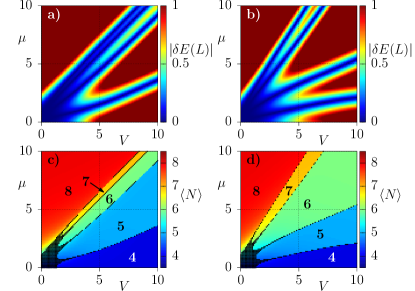
Figure S2: Results for $L=8$, $\Delta=1$ and $W=0$ (a,c) or $W=V/2$ (b,d). a) and b) Difference between the ground state energies obtained for different parities of fermions, $\delta E(L)$. c) and d) Average occupation of fermions in the ground state. Points mark parameters for which $|\delta E(L)|<0.02$.

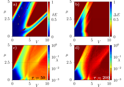
Figure S3: The same as in Fig. 3 in the main text, but for $W=0$.

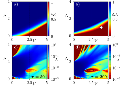
Figure S4: The same as in Fig. 4 in the main text, but for $W=0$. Point in b) marks exact boundary of the topological phase from Ref. Katsura et al. (2015).

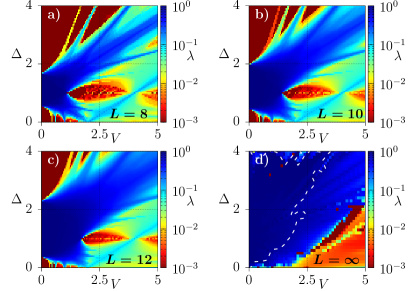
Figure S5: The same as Fig. 5 in the main text but for $W=0$.

Figures S3, S4 and S5 show respectively the same phase diagrams as Figs. 3, 4 and 5 in the main text but for $W=0$. These phase diagrams are constructed from the Majorana autocorrelation function $\lambda$. On the one hand, these plots clearly show that the qualitative results discussed in the main text are generic, i.e., they are independent of a specific choice of the many–body interaction. The main message is that the long–living Majorana modes exist not only in the ground state but within the whole energy spectrum for moderate interactions, while weak interaction may even expand the range of the chemical potential where these modes exist (see Figs. S3c and S3d). On the other hand, the phase diagrams for $W=0$ include rather complicated structure of lines where Majorana modes are particularly robust, see e.g., Figs. S4d and S5a-S5c. However, such structures are not generic because they don’t show up for $W\neq 0$.

IV Details of the finite-size scaling

As argued in the main text, it is utterly important for systems with hard–wall boundary conditions that the thermodynamic limit $L\rightarrow\infty$ precedes the limit $\tau\rightarrow\infty$. It means that the correct finite–size (FS) scaling should be carried out not for a single quantity but for the $\tau$–dependent Majorana autocorrelation function $\lambda(\tau)$. In order to efficiently perform such scaling, we first fit $\lambda(\tau)$ for a given system length $L$ and then carry out the FS scaling for the fitting parameters. It is convenient to start from a standard time–dependent correlation function

$$\langle\Gamma(t)\Gamma\rangle=\frac{1}{Z}\sum_{m,n}\exp[it(E_{m}-E_{n})]|\langle n|\Gamma|m\rangle|^{2},$$ (S14)

It differs from the $\tau$–dependent autocorrelation functions $\langle\bar{\Gamma}\Gamma\rangle$ which utilizes time–averaging introduced in Eq. (2) in the main text. However, the relation between both functions can be easily established

$$\langle\bar{\Gamma}\Gamma\rangle = \frac{1}{Z}\sum_{m,n}\theta\left(\frac{1}{\tau}-|E_{m}-E_{n}|\right)|\langle n|\Gamma|m\rangle|^{2}$$ (S15)

$$= \frac{1}{Z}\sum_{m,n}|\langle n|\Gamma|m\rangle|^{2}\int_{-1/\tau}^{1/\tau}\mathrm{d}\omega\;\delta(\omega+E_{m}-E_{n})$$

$$= \frac{1}{2\pi}\int_{-1/\tau}^{1/\tau}\mathrm{d}\omega\int_{-\infty}^{\infty}\mathrm{d}te^{i\omega t}\langle\Gamma(t)\Gamma\rangle.$$

One immediately finds the limit

$$\lim_{\tau\rightarrow\infty}\langle\bar{\Gamma}\Gamma\rangle=\frac{1}{Z}\sum_{m,n:E_{m}=E_{n}}|\langle n|\Gamma|m\rangle|^{2}.$$

This limit is exactly equal to the steady–state part of $\langle\Gamma(t)\Gamma\rangle$ [see Eq. (S14)] which survives for arbitrarily large $t$. For finite $\tau$, $\langle\bar{\Gamma}\Gamma\rangle$ represents the integrated low–frequency part of the Fourier transform of $\langle\Gamma(t)\Gamma\rangle$, as follows from the last line in Eq. (S15). We use $\langle\bar{\Gamma}\Gamma\rangle$ instead of $\langle\Gamma(t)\Gamma\rangle$ because only the former function is monotonic. It filters out the oscillations of $\langle\Gamma(t)\Gamma\rangle$ but retains essential information about the asymptotic long–time behavior Prelovšek et al. (2017). But most importantly, the efficiency of our method follows from that the specific time–averaging, $\bar{\Gamma}$, is an orthogonal projection also for $\tau<\infty$, i.e., $\langle\bar{\Gamma}\Gamma\rangle=\langle\bar{\Gamma}\bar{\Gamma}\rangle$. The latter identity can be checked, by direct calculations. Namely, using Eq. (3) from the main text, one obtains

$$\langle\bar{\Gamma}\bar{\Gamma}\rangle = \frac{1}{Z}\sum_{m,n}\left[\theta\left(\frac{1}{\tau}-|E_{m}-E_{n}|\right)\langle n|\Gamma|m\rangle\right.$$ (S16)

$$\left.\theta\left(\frac{1}{\tau}-|E_{n}-E_{m}|\right)\langle m|\Gamma|n\rangle\right].$$

Since both $\theta$–functions have equal arguments and $\theta^{2}(x)=\theta(x)$ one obtains a formula that is identical to the first line in Eq. (S15).

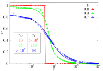
Figure S6: The Majorana autocorrelation function $\lambda$ for various times $\tau$. Points show numerical results for $L=12$, $\Delta=0.3$, $\mu=0$ and $W=V/2$ while continuous lines show best fits, given by Eq. (LABEL:cfit). The scattering times, $\tau_{M}$ and $\tau_{I}$, are shown in the table.

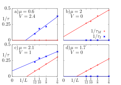
Figure S7: Representative examples for the finite–size scaling of scattering times, $\tau_{I}$ and $\tau_{M}$ for $\Delta=1$, $W=0$.

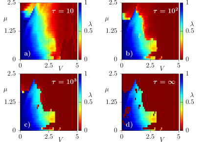
Figure S8: Extrapolated Majorana autocorrelation function, $\lim_{L\rightarrow\infty}\lambda$ for $\Delta=1$, $W=0$ various times $\tau$.

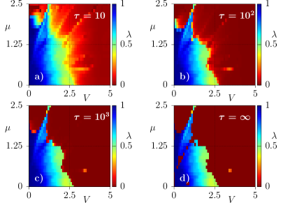
Figure S9: The same as in Fig. S8 but for $W=V/2$.

In order to find the relevant fitting function for $\lambda(\tau)$, we notice that generic many–body interactions are expected to cause exponential decay of correlations functions. It holds true also for perturbed integrable systems Mierzejewski et al. (2015b). For $\langle\Gamma(t)\Gamma\rangle=\exp(-t/\tau_{I})$ one obtains from Eq. (S15)

$$\langle\bar{\Gamma}\Gamma\rangle = \frac{2}{\pi}\arctan\left(\frac{\tau_{I}}{\tau}\right).$$ (S17)

However, such form is too simple to account for finite noninteracting systems, where the Majorana lifetime, $\tau_{M}$, is limited by the overlap of Majorana modes at two ends of the chain. Without interactions, the Majorana autocorrelation function is a step function, as shown in Fig. 1a in the main text. In order to accommodate this mechanism we have modified Eq. (S17)

$$\lambda_{\mathrm{fit}}(\tau) = \frac{C}{\pi}\left[\arctan\left(\frac{\tau_{\mathrm{I}}}{\tau}-\frac{\tau_{\mathrm{I}}}{\tau_{M}}\right)+\arctan\left(\frac{\tau_{\mathrm{I}}}{\tau}+\frac{\tau_{\mathrm{I}}}{\tau_{M}}\right)\right].$$

The fitting function contains three parameters: $C$, $\tau_{\mathrm{I}}$ and $\tau_{M}$. Here, $1/\tau_{M}$ and $1/\tau_{\mathrm{I}}$ represent scattering rates due to the overlap of two Majorana modes and due to the many–body interactions, respectively. If the relaxation is dominated by the many–body interactions, then $\lim_{\tau_{M}\rightarrow\infty}\lambda_{\mathrm{fit}}(\tau)=\frac{2C}{\pi}\arctan\left(\frac{\tau_{\mathrm{I}}}{\tau}\right)$. However, if the relaxation is due to overlap of two Majorana modes, then $\lim_{\tau_{\mathrm{I}}\rightarrow\infty}\lambda_{\mathrm{fit}}(\tau)=C\theta(\tau_{M}-\tau)$, in agreement with Fig. 1a in the main text. Figure S6 shows that $\lambda(\tau)$ may be well fitted by Eq. (LABEL:cfit) also for intermediate cases, when both scattering mechanisms are important.

In Fig. S7 we show a few representative examples for the finite size scaling of the scattering rates $1/\tau_{\mathrm{I}}$ and $1/\tau_{M}$. One is mostly interested in the case when both scattering rates vanish in the thermodynamic limit (see Figs. S7a, S7d) and $\lim_{\tau\rightarrow\infty}\lim_{L\rightarrow\infty}\lambda(\tau)=\lim_{L\rightarrow\infty}C$. Otherwise, $\lim_{\tau\rightarrow\infty}\lim_{L\rightarrow\infty}\lambda(\tau)=0$ if one of the scattering times remain finite. In noninteracting system, the Majorana modes exist for $|\mu|<2$ what is correctly reproduced by our approach as shown in Figs. S7b and S7d.

After the FS scaling has been accomplished, one may study (approximate) results for the Majorana autocorrelation function in the thermodynamic limit presented in Figs. S8 and S9. These plots show $\lambda_{\mathrm{fit}}(\tau)$ where all fitting parameters are replaced by their extrapolated values. Such procedure unavoidably introduces errors. Consequently the irregular shape of the regime with Majorana modes most probably arises as a numerical artifacts. Nevertheless, it is rather evident that the information stored in the Majorana autocorrelation functions is at least partially retained for arbitrarily long times also for rather strong interactions $V\lesssim 2$. However, if the Majorana modes are strict integrals of motion then $\lim_{\tau\rightarrow\infty}\lim_{L\rightarrow\infty}\lambda(\tau)=1$. Numerical results shown in Figs. S8 and S9 strongly suggest that in the presence of many–body interactions, the latter limit is always smaller than unity, even though it may be very close to this value. As argued in the main text, this implies the presence of quasilocal strictly conserved operators $\lim_{\tau\rightarrow\infty}\bar{\Gamma}$, which have large projection on strictly local Majorana modes, $\Gamma$.

The method has been demonstrated for a toy model of spinless fermions with $p$–wave pairing. This model, however, is a prototype on which all current 1D realizations of Majorana physics are based Lutchyn et al. (2010); Oreg et al. (2010). In real systems, the Zeeman splitting is used to break the Kramers degeneracy and create effectively spinless fermions. The Rashba spin–orbit coupling combined with $s$–wave pairing induced by proximity to a conventional superconductor produces effective $p$–wave pairing. Then, in order to enter the topological phase that guarantees the presence of Majorana end modes, the parameters of the realistic model (Zeeman splitting $V_{Z}$, chemical potential $\mu$ and superconducting gap magnitude $\Delta$) have to satisfy exactly the same relation as derived for the Kitaev chain: $V_{Z}>\sqrt{\Delta^{2}+\mu^{2}}$ Franz (2013). Moreover, the proposed method can be straightforwardly applied to models of the semiconducting nanowires used in real experiments. The only problem is that for spinful electrons the Hilbert space is twice as large as in the Kitaev model, what would limit the maximum length of the system. And since the lifetime of MZM increases with the system size, we preferred our system to be as large as possible.

References

- Aasen et al. (2016) David Aasen, Michael Hell, Ryan V. Mishmash, Andrew Higginbotham, Jeroen Danon, Martin Leijnse, Thomas S. Jespersen, Joshua A. Folk, Charles M. Marcus, Karsten Flensberg, and Jason Alicea, “Milestones toward Majorana-based quantum computing,” Phys. Rev. X 6, 031016 (2016).
- Sarma et al. (2015) Sankar Das Sarma, Michael Freedman, and Chetan Nayak, “Majorana zero modes and topological quantum computation,” npj Quantum Information 1, 15001 (2015).
- Karzig et al. (2017) Torsten Karzig, Christina Knapp, Roman M. Lutchyn, Parsa Bonderson, Matthew B. Hastings, Chetan Nayak, Jason Alicea, Karsten Flensberg, Stephan Plugge, Yuval Oreg, Charles M. Marcus, and Michael H. Freedman, “Scalable designs for quasiparticle-poisoning-protected topological quantum computation with Majorana zero modes,” Phys. Rev. B 95, 235305 (2017).
- Plugge et al. (2016) S. Plugge, L. A. Landau, E. Sela, A. Altland, K. Flensberg, and R. Egger, “Roadmap to Majorana surface codes,” Phys. Rev. B 94, 174514 (2016).
- Akhmerov (2010) A. R. Akhmerov, “Topological quantum computation away from the ground state using Majorana fermions,” Phys. Rev. B 82, 020509 (2010).
- Lutchyn et al. (2010) Roman M. Lutchyn, Jay D. Sau, and S. Das Sarma, “Majorana fermions and a topological phase transition in semiconductor-superconductor heterostructures,” Phys. Rev. Lett. 105, 077001 (2010).
- Oreg et al. (2010) Yuval Oreg, Gil Refael, and Felix von Oppen, “Helical liquids and majorana bound states in quantum wires,” Phys. Rev. Lett. 105, 177002 (2010).
- Franz (2013) Marcel Franz, “Majorana’s wires,” Nat. Nanotechnol 8, 149–152 (2013).
- Mourik et al. (2012) V. Mourik, K. Zuo, S. M. Frolov, S. R. Plissard, E. P. A. M. Bakkers, and L. P. Kouwenhoven, “Signatures of Majorana fermions in hybrid superconductor-semiconductor nanowire devices,” Science 336, 1003 (2012).
- Nadj-Perge et al. (2014) Stevan Nadj-Perge, Ilya K. Drozdov, Jian Li, Hua Chen, Sangjun Jeon, Jungpil Seo, Allan H. MacDonald, B. Andrei Bernevig, and Ali Yazdani, “Observation of Majorana fermions in ferromagnetic atomic chains on a superconductor,” Science 346, 602 (2014).
- Pawlak et al. (2016) Rémy Pawlak, Marcin Kisiel, Jelena Klinovaja, Tobias Meier, Shigeki Kawai, Thilo Glatzel, Daniel Loss, and Ernst Meyer, “Probing atomic structure and Majorana wavefunctions in mono-atomic fe chains on superconducting pb surface,” npj Quantum Information 2, 16035 (2016).
- Ruby et al. (2015) Michael Ruby, Falko Pientka, Yang Peng, Felix von Oppen, Benjamin W. Heinrich, and Katharina J. Franke, “End states and subgap structure in proximity-coupled chains of magnetic adatoms,” Phys. Rev. Lett. 115, 197204 (2015).
- Haldane (1981) D. M. Haldane, “’Luttinger liquid theory’ of one-dimensional quantum fluids. I. Properties of the Luttinger model and their extension to the general 1D interacting spinless Fermi gas,” J. Physics C. 14, 2585 (1981).
- Gangadharaiah et al. (2011) Suhas Gangadharaiah, Bernd Braunecker, Pascal Simon, and Daniel Loss, “Majorana edge states in interacting one-dimensional systems,” Phys. Rev. Lett. 107, 036801 (2011).
- Manolescu et al. (2014) A. Manolescu, D. C. Marinescu, and T. D. Stanescu, “Coulomb interaction effects on the Majorana states in quantum wires,” J. Physics. Condens. Matter 26, 172203 (2014).
- Vuik et al. (2016) A. Vuik, D. Eeltink, A. R. Akhmerov, and M Wimmer, “Effects of the electrostatic environment on the Majorana nanowire devices,” New J. Phys. 18, 033013 (2016).
- Domínguez et al. (2017a) Fernando Domínguez, Jorge Cayao, Pablo San-Jose, Ramón Aguado, Alfredo Levy Yeyati, and Elsa Prada, “Zero-energy pinning from interactions in majorana nanowires,” npj Quantum Materials 2, 13 (2017a).
- Maśka et al. (2017) Maciej M. Maśka, Anna Gorczyca-Goraj, Jakub Tworzydło, and Tadeusz Domański, “Majorana quasiparticles of an inhomogeneous rashba chain,” Phys. Rev. B 95, 045429 (2017).
- Lutchyn et al. (2011) Roman M. Lutchyn, Tudor D. Stanescu, and S. Das Sarma, “Search for Majorana fermions in multiband semiconducting nanowires,” Phys. Rev. Lett. 106, 127001 (2011).
- Akhmerov et al. (2011) A. R. Akhmerov, J. P. Dahlhaus, F. Hassler, M. Wimmer, and C. W. J. Beenakker, “Quantized conductance at the Majorana phase transition in a disordered superconducting wire,” Phys. Rev. Lett. 106, 057001 (2011).
- Domínguez et al. (2017b) Fernando Domínguez, Jorge Cayao, Pablo San-Jose, Ramón Aguado, Alfredo Levy Yeyati, and Elsa Prada, “Zero-energy pinning from interactions in Majorana nanowires,” npj Quantum Materials 2, 13 (2017b).
- Stoudenmire et al. (2011) E. M. Stoudenmire, Jason Alicea, Oleg A. Starykh, and Matthew P.A. Fisher, “Interaction effects in topological superconducting wires supporting Majorana fermions,” Phys. Rev. B 84, 014503 (2011).
- Gergs et al. (2016) Niklas M. Gergs, Lars Fritz, and Dirk Schuricht, “Topological order in the Kitaev/Majorana chain in the presence of disorder and interactions,” Phys. Rev. B 93, 075129 (2016).
- Hassler and Schuricht (2012) Fabian Hassler and Dirk Schuricht, “Strongly interacting Majorana modes in an array of josephson junctions,” New J. Phys. 14, 125018 (2012).
- Nayak et al. (2008) Chetan Nayak, Steven H. Simon, Ady Stern, Michael Freedman, and Sankar Das Sarma, “Non-abelian anyons and topological quantum computation,” Rev. Mod. Phys. 80, 1083 (2008).
- Clarke et al. (2011) David J. Clarke, Jay D. Sau, and Sumanta Tewari, “Majorana fermion exchange in quasi-one-dimensional networks,” Phys. Rev. B 84, 035120 (2011).
- Kitaev (2001) A Yu Kitaev, “Unpaired Majorana fermions in quantum wires,” Phys. Usp. 44, 131 (2001).
- Kells (2015) G. Kells, “Many-body Majorana operators and the equivalence of parity sectors,” Phys. Rev. B 92, 081401 (2015).
- Ng (2015) H. T. Ng, “Decoherence of interacting Majorana modes,” Sci. Rep. 5, 12530 (2015).
- Su et al. (2016) W. Su, M. N. Chen, L. B. Shao, L. Sheng, and D. Y. Xing, “Electron-electron interaction effects in floquet topological superconducting chains: Suppression of topological edge states and crossover from weak to strong chaos,” Phys. Rev. B 94, 075145 (2016).
- Chan et al. (2015) Y.-H. Chan, Ching-Kai Chiu, and Kuei Sun, “Multiple signatures of topological transitions for interacting fermions in chain lattices,” Phys. Rev. B 92, 104514 (2015).
- Hofmann et al. (2016) Johannes S. Hofmann, Fakher F. Assaad, and Andreas P. Schnyder, “Edge instabilities of topological superconductors,” Phys. Rev. B 93, 201116 (2016).
- Thomale et al. (2013) Ronny Thomale, Stephan Rachel, and Peter Schmitteckert, “Tunneling spectra simulation of interacting Majorana wires,” Phys. Rev. B 88, 161103 (2013).
- Chen et al. (2011) Xie Chen, Zheng-Cheng Gu, and Xiao-Gang Wen, “Classification of gapped symmetric phases in one-dimensional spin systems,” Phys. Rev. B 83, 035107 (2011).
- Fidkowski and Kitaev (2010) Lukasz Fidkowski and Alexei Kitaev, “Effects of interactions on the topological classification of free fermion systems,” Phys. Rev. B 81, 134509 (2010).
- Katsura et al. (2015) Hosho Katsura, Dirk Schuricht, and Masahiro Takahashi, “Exact ground states and topological order in interacting Kitaev/Majorana chains,” Phys. Rev. B 92, 115137 (2015).
- Alicea and Fendley (2016) Jason Alicea and Paul Fendley, “Topological phases with parafermions: Theory and blueprints,” Annu. Rev. of Condens. Matter Phys. 7, 119–139 (2016).
- Else et al. (2017) Dominic V. Else, Paul Fendley, Jack Kemp, and Chetan Nayak, “Prethermal strong zero modes and topological qubits,” Phys. Rev. X 7, 041062 (2017).
- Goldstein and Chamon (2012) G. Goldstein and C. Chamon, “Exact zero modes in closed systems of interacting fermions,” Phys. Rev. B 86, 115122 (2012).
- Kemp et al. (2017) Jack Kemp, Norman Y Yao, Christopher R Laumann, and Paul Fendley, “Long coherence times for edge spins,” J. Stat. Mech. 2017, P063105 (2017).
- (41) Also, within the proposed approach, terms including three or more ’s can (and in a general case should) be taken into account. We have checked at least for at least a few paprameter sets that the contribution from terms with three ’s is negligible.
- (42) See Supplemental Material at [URL will be inserted by publisher] for the details of the finite size scaling, results for nearest-neighbor interaction, and more formal discussion of the Majorana zero modes.
- Fendley (2016) Paul Fendley, “Strong zero modes and eigenstate phase transitions in the XYZ/interacting Majorana chain,” J. Phys. A 49, 30LT01 (2016).
- Jermyn et al. (2014) Adam S. Jermyn, Roger S. K. Mong, Jason Alicea, and Paul Fendley, “Stability of zero modes in parafermion chains,” Phys. Rev. B 90, 165106 (2014).
- Mierzejewski et al. (2015a) Marcin Mierzejewski, Peter Prelovšek, and Tomaž Prosen, “Identifying local and quasilocal conserved quantities in integrable systems,” Phys. Rev. Lett. 114, 140601 (2015a).
- (46) T. E. O’Brien and A. R. Wright, “A many-body interpretation of Majorana bound states, and conditions for their localisation,” arXiv:1508.06638 .
- Rigol and Shastry (2008) Marcos Rigol and B. S. Shastry, “Drude weight in systems with open boundary conditions,” Phys. Rev. B 77, 161101 (2008).
- Sirker et al. (2014) J. Sirker, N. P. Konstantinidis, F. Andraschko, and N. Sedlmayr, “Locality and thermalization in closed quantum systems,” Phys. Rev. A 89, 042104 (2014).
- Mierzejewski et al. (2015b) Marcin Mierzejewski, Tomaž Prosen, and Peter Prelovšek, “Approximate conservation laws in perturbed integrable lattice models,” Phys. Rev. B 92, 195121 (2015b).
- Prelovšek et al. (2017) P. Prelovšek, M. Mierzejewski, O. Barišič, and J. Herbrych, “Density correlations and transport in models of many-body localization,” Ann. Phys. (Amsterdam) 529 (2017).
- Miao et al. (2017) Jian-Jian Miao, Hui-Ke Jin, Fu-Chun Zhang, and Yi Zhou, “Exact solution for the interacting Kitaev chain at the symmetric point,” Phys. Rev. Lett. 118, 267701 (2017).