Bellman Gradient Iteration for Inverse Reinforcement Learning

Abstract

This paper develops an inverse reinforcement learning algorithm aimed at recovering a reward function from the observed actions of an agent. We introduce a strategy to flexibly handle different types of actions with two approximations of the Bellman Optimality Equation, and a Bellman Gradient Iteration method to compute the gradient of the Q-value with respect to the reward function. These methods allow us to build a differentiable relation between the Q-value and the reward function and learn an approximately optimal reward function with gradient methods. We test the proposed method in two simulated environments by evaluating the accuracy of different approximations and comparing the proposed method with existing solutions. The results show that even with a linear reward function, the proposed method has a comparable accuracy with the state-of-the-art method adopting a non-linear reward function, and the proposed method is more flexible because it is defined on observed actions instead of trajectories

I introduction

In many problems, the actions of an agent in an environment can be modeled as a Markov Decision Process, where the environment decides the states and transitional probabilities, and the agent decides its own reward function based on the preferences over the states and takes actions accordingly. Since the agent’s reward function determines its actions, it is possible to estimate the state preferences from the observed actions, hence the inverse reinforcement learning problem.

This problem arises in many applications. For example, in robot learning by demonstration [1], an operator may manipulate an object based on knowledge and preference of the object, like which object states are achievable and which object states are desired. By learning the knowledge and preference from the observed operator motion, a robot can manipulate the object in an appropriate way. Another application is analyzing a person’s physical wellness from daily observation of motions. Assuming the person’s actions are based on self-evaluation of physical limitations, the change of such limitations (a potential sign of health problems) can be reflected by long-term monitoring of the subject’s motion and estimated via inverse reinforcement learning (IRL).

To solve the problem, it is critical to model the relation between the agent’s actions and the reward functions. Since an action depends on both the immediate reward and future rewards, existing solutions model either a relation between the actions and the value function [2, 3], or a relation between the actions and the Q-function [4, 5, 6, 7]. To efficiently compute the optimal reward function, the gradient of the optimal value function and the optimal Q-function with respect to the reward function parameter is necessary, but the optimal value function and optimal Q function are non-differentiable with respect to the rewards, and existing solutions adopt different approximations to alleviate the problem.

This paper introduces two approximations of the Bellman Optimality Equation to make the optimal value function and the optimal Q-function differentiable with respect to the reward function, and proposes a Bellman Gradient Iteration method to compute the gradients efficiently. The approximation level can be adjusted with a parameter to adapt to different types of action preferences, like preferring an action leading to an optimal future path, or an action leading to uncertain future paths. To the best of our knowledge, no previous work computes the gradients by modeling the relation between motion and reward in a differentiable way.

The paper is organized as follows. We review existing work on inverse reinforcement learning in Section II, and formulate the gradient-based method in Section III. We introduce Bellman Gradient Iteration method to compute the gradients in Section IV. Several experiments are shown in Section V, with conclusions in Section VI.

II Related Works

The Inverse Reinforcement Learning problem is first formulated in [5], where the agent observes the states resulting from an assumingly optimal policy, and tries to learn a reward function that makes the policy better than all alternatives. Since the goal can be achieved by multiple reward functions, this paper tries to find one that maximizes the difference between the observed policy and the second best policy. This idea is extended by [6], in the name of max-margin learning for inverse optimal control. Another extension is proposed in [3], where the goal is not to recover the actual reward function, but to find a reward function that leads to a policy equivalent to the observed one, measured by the total reward collected by following that policy.

Since a motion policy may be difficult to estimate from observations, a behavior-based method is proposed in [2], which models the distribution of behaviors as a maximum-entropy model on the amount of reward collected from each behavior. This model has many applications and extensions. For example, Nguyen et al. [8] consider a sequence of changing reward functions instead of a single reward function. Levine et al. [9] and Finn et al. [10] consider complex reward functions, instead of linear ones, and use Gaussian process and neural networks, respectively, to model the reward function. Choi et al. [11] consider partially observed environments, and combines partially observed Markov Decision Process with reward learning. Levine et al. [12] model the behaviors based on the local optimality of a behavior, instead of the summation of rewards. Wulfmeier et al. [13] use a multi-layer neural network to represent nonlinear reward functions.

Another method is proposed in [4], which models the probability of a behavior as the product of each state-action’s probability, and learns the reward function via maximum a posteriori estimation. However, due to the complex relation between the reward function and the behavior distribution, the author uses computationally expensive Monte-Carlo methods to sample the distribution. This work is extended by [7], which uses sub-gradient methods to reduce the computations. Another extensions is shown in [14], which tries to find a reward function that matches the observed behavior. For motions involving multiple tasks and varying reward functions, methods are developed in [15] and [16], which try to learn multiple reward functions.

Our method uses gradient methods like [7], but we introduce two approximation methods that improve the flexibility of motion modeling, and a Bellman Gradient Iteration algorithm that computes the gradient of the optimal value function and the optimal Q-function with respect to the reward function accurately and efficiently.

III Inverse Reinforcement Learning

III-A Markov Decision Process

A Markov Decision Process is described with the following variables:

• $S=\{s\}$, a set of states

• $A=\{a\}$, a set of actions

• $P_{ss^{\prime}}^{a}$, a state transition function that defines the probability that state $s$ becomes $s^{\prime}$ after action $a$.

• $R=\{r(s)\}$, a reward function that defines the immediate reward of state $s$.

• $\gamma$, a discount factor that ensures the convergence of the MDP over an infinite horizon.

A motion can be represented as a sequence of state-action pairs:

$$\zeta=\{(s_{i},a_{i})|i=0,\cdots,N_{\zeta}\}$$

where $N_{\zeta}$ denotes the length of the motion.

One key problem is how to choose the action in each state, or the policy, $\pi(s)\in A$, a mapping from states to actions. This problem can be handled by reinforcement learning algorithms, by introducing the value function $V(s)$ and the Q-function $Q(s,a)$, described by the Bellman Equation [17]:

$$V^{\pi}(s)=\sum_{s^{\prime}|s,\pi(s)}P_{ss^{\prime}}^{\pi(s)}[r(s^{\prime})+\gamma*V^{\pi}(s^{\prime})],$$ (1)

$$Q^{\pi}(s,a)=\sum_{s^{\prime}|s,a}P_{ss^{\prime}}^{a}[r(s^{\prime})+\gamma*V^{\pi}(s^{\prime})]$$ (2)

where $V^{\pi}$ and $Q^{\pi}$ define the value function and the Q-function under a policy $\pi$.

For an optimal policy $\pi^{*}$, the value function and the Q-function should be maximized on every state. This is described by the Bellman Optimality Equation [17]:

$$V^{*}(s)=\max_{a\in A}\sum_{s^{\prime}|s,a}P_{ss^{\prime}}^{a}[r(s^{\prime})+\gamma*V^{*}(s^{\prime})],$$ (3)

$$Q^{*}(s,a)=\sum_{s^{\prime}|s,a}P_{ss^{\prime}}^{a}[r(s^{\prime})+\gamma*\max_{a^{\prime}\in A}Q^{*}(s^{\prime},a^{\prime})].$$ (4)

With the optimal value function, $V^{*}(s)$, and Q-function, $Q^{*}(s,a)$, the action $a$ for state $s$ can be chosen in multiple ways. For example, the agent may choose $a$ in a stochastic way:

$$P(a|s)\propto Q^{*}(s,a),a\in A$$

where the agent’s probability to choose action $a$ in state $s$ is proportional to the optimal Q value $Q^{*}(s,a)$.

III-B Motion Modeling

Assuming the reward function $r$ is parameterized by $\theta$, we model $P(\zeta|\theta)$ based on the optimal Q-value of each state-action pair of $\zeta=\{(s_{i},a_{i})|i=0,\cdots,N_{\zeta}\}$:

$$P(\zeta|\theta)=\prod_{(s,a)\in\zeta}P((s,a)|\theta)$$ (5)

where

$$P((s,a)|\theta)=\frac{\exp{b*Q^{*}(s,a)}}{\sum_{\hat{a}\in A}\exp{b*Q^{*}(s,\hat{a})}}$$ (6)

defines the probability to choose action $a$ in state $s$ based on the formulation in [4], and $b$ is a parameter controlling the degree of confidence in the agent’s ability to choose actions based on Q values. In the remaining sections, we use $Q(s,a)$ to denote the optimal Q-value of the state-action pair $(s,a)$. Since $Q(s,a)$ depends on reward function $r$, it also depends on $\theta$.

In this formulation, the inverse reinforcement learning problem is equivalent to maximum-likelihood estimation of $\theta$:

$$\theta=\operatorname*{argmax}_{\theta}\log{P(\zeta|\theta)}$$ (7)

where the log-likelihood of $P(\zeta|\theta)$ is given by:

$$L(\theta)=\sum_{(s,a)\in\zeta}(b*Q(s,a)-\log{\sum_{\hat{a}\in A}\exp{b*Q(s,\hat{a}))}}$$ (8)

and the gradient of the log-likelihood is given by:

$$\nabla L(\theta) =\sum_{(s,a)\in\zeta}(b*\nabla Q(s,a)$$

$$-b*\sum_{\hat{a}\in A}P((s,\hat{a})|r(\theta))\nabla Q(s,\hat{a})).$$ (9)

If we can compute the gradient of the Q-function $\nabla Q=\frac{\partial Q}{\partial\theta}=\frac{\partial Q}{\partial r}\cdot\frac{\partial r}{\partial\theta}$, we can use gradient methods to find a locally optimal parameter value:

$$\theta=\theta+\alpha*\nabla L(\theta)$$ (10)

where $\alpha$ is the learning rate. When the reward function is linear, the cost function is convex and the global optimum can be achieved. The standard way to compute the optimal Q-value is with the following Bellman Equation of Optimality [17] with Equation (4).

However, the Q-value in Equation (4) is non-differentiable with respect to $r$ or $\theta$ due to the max operator. Its gradient $\nabla Q(s,a)$ cannot be computed in a conventional way, and the sub-gradient method in [7] cannot compute the gradients everywhere in the parameter space. We propose a method called Bellman Gradient Iteration to solve the problem.

IV Bellman Gradient Iteration

To handle the non-differentiable max function in Equation (4), we introduce two approximation methods.

IV-A Approximation with a P-Norm Function

The first approximation is based on a p-norm:

$$\max(a_{0},\cdots,a_{n})\approx(\sum_{i=0}^{n}a_{i}^{k})^{\frac{1}{k}}$$ (11)

where $k$ controls the level of approximation, and we assume all the values $a_{0},\cdots,a_{n}$ are positive. When $k=\infty$, the approximation becomes exact. In the remaining section, we refer to this method as p-norm approximation.

Under this approximation, the Q-function in Equation (4) can be rewritten as:

$$Q_{p}(s,a)=\sum_{s^{\prime}|s,a}P_{ss^{\prime}}^{a}[r(s^{\prime})+\gamma*(\sum_{a^{\prime}\in A}Q_{p}^{k}(s^{\prime},a^{\prime}))^{1/k}].$$ (12)

From Equation (12), we construct an approximately optimal value function with p-norm approximation:

$$V_{p}(s)=(\sum_{a\in A}Q_{p}^{k}(s,a))^{1/k}.$$ (13)

Using Equations (12) and (13), we build an approximate Bellman Optimality Equation to find the approximately optimal value function and Q-function:

$$Q_{p}(s,a)=\sum_{s^{\prime}|s,a}P_{ss^{\prime}}^{a}[r(s^{\prime})+\gamma*V_{p}(s^{\prime})],$$ (14)

$$V_{p}(s)=(\sum_{a\in A}(\sum_{s^{\prime}|s,a}P_{ss^{\prime}}^{a}[r(s^{\prime})+\gamma*V_{p}(s^{\prime})]))^{k})^{1/k}.$$ (15)

Taking derivative on both sides of Equation (13) and Equation (14), we construct a Bellman Gradient Equation to compute the gradients of $V_{p}(s)$ and $Q_{p}(s,a)$ with respect to reward function parameter $\theta$:

$$\frac{\partial V_{p}(s)}{\partial\theta}=\frac{1}{k}(\sum_{a\in A}Q_{p}^{k}(s,a))^{\frac{1-k}{k}}\sum_{a\in A}k*Q_{p}^{k-1}(s,a)\frac{\partial Q_{p}(s,a)}{\partial\theta},$$ (16)

$$\frac{\partial Q_{p}(s,a)}{\partial\theta}=\sum_{s^{\prime}|s,a}P_{ss^{\prime}}^{a}(\frac{\partial r(s^{\prime})}{\partial\theta}+\gamma*\frac{\partial V_{p}(s^{\prime})}{\partial\theta}).$$ (17)

For a p-norm approximation with non-negative Q-values, the gap between the approximate value function and the optimal value function is a function of $k$:

$$g_{p}(k)=(\sum_{a^{\prime}\in A}Q_{p}(s^{\prime},a^{\prime})^{k})^{\frac{1}{k}}-\max_{a^{\prime}\in A}Q_{p}(s^{\prime},a^{\prime}).$$

The gap function $g_{p}(k)$ describes the error of the approximation, and it has two properties.

Theorem 1

Assuming all Q-values are non-negative, $Q_{p}(s,a)\geq 0,\forall s,a$, the tight lower bound of $g_{p}(k)$ is zero:

$$\inf_{\forall k\in R}g_{p}(k)=0.$$

Proof:

$\forall k\in R$, assuming $a_{max}=\operatorname*{argmax}_{a^{\prime}\in A}Q_{p}(s^{\prime},a^{\prime}),$

$$g_{p}(k) =(\sum_{a^{\prime}\in A}Q_{p}(s^{\prime},a^{\prime})^{k})^{\frac{1}{k}}-\max_{a^{\prime}\in A}Q_{p}(s^{\prime},a^{\prime})$$

$$=(\sum_{a^{\prime}\in A/a_{max}}Q_{p}(s^{\prime},a^{\prime})^{k}+Q_{p}(s^{\prime},a_{max})^{k})^{\frac{1}{k}}-\max_{a^{\prime}\in A}Q_{p}(s^{\prime},a^{\prime}).$$

Since $Q_{p}(s,a)\geq 0\Rightarrow\sum_{a^{\prime}\in A/a_{max}}Q_{p}(s^{\prime},a^{\prime})^{k}\geq 0$,

$$g_{p}(k) \geq(Q_{p}(s^{\prime},a_{max})^{k})^{\frac{1}{k}}-\max_{a^{\prime}\in A}Q_{p}(s^{\prime},a^{\prime})$$

$$=Q_{p}(s^{\prime},a_{max})-\max_{a^{\prime}\in A}Q_{p}(s^{\prime},a^{\prime})=0$$

When $k=\infty$:

$$g_{p}(k) =(\sum_{a^{\prime}\in A}Q_{p}(s^{\prime},a^{\prime})^{\infty})^{\frac{1}{\infty}}-\max_{a^{\prime}\in A}Q_{p}(s^{\prime},a^{\prime})$$

$$=\max_{a^{\prime}\in A}Q_{p}(s^{\prime},a^{\prime})-\max_{a^{\prime}\in A}Q_{p}(s^{\prime},a^{\prime})=0$$

∎

Theorem 2

Assuming all Q-values are non-negative, $Q_{p}(s,a)\geq 0,\forall s,a$, $g_{p}(k)$ is a decreasing function with respect to $k$:

$$g^{\prime}_{p}(k)\leq 0,\forall k\in R.$$

Proof:

$$g^{\prime}_{p}(k) =\frac{1}{k}*(\sum_{a^{\prime}\in A}Q_{p}(s^{\prime},a^{\prime})^{k})^{\frac{1-k}{k}}*(\sum_{a^{\prime}\in A}Q_{p}(s^{\prime},a^{\prime})^{k}\log(Q_{p}(s^{\prime},a^{\prime})))$$

$$+(\sum_{a^{\prime}\in A}Q_{p}(s^{\prime},a^{\prime})^{k})^{\frac{1}{k}}\log(\sum_{a^{\prime}\in A}Q_{p}(s^{\prime},a^{\prime})^{k})\frac{1}{-k^{2}}$$

$$=\frac{(\sum_{a^{\prime}\in A}Q_{p}(s^{\prime},a^{\prime})^{k})^{\frac{1}{k}}}{k^{2}\sum_{a^{\prime}\in A}Q_{p}(s^{\prime},a^{\prime})^{k}}(\sum_{a^{\prime}\in A}Q_{p}(s^{\prime},a^{\prime})^{k}k\log(Q_{p}(s^{\prime},a^{\prime}))$$

$$-\sum_{a^{\prime}\in A}Q_{p}(s^{\prime},a^{\prime})^{k}\log(\sum_{a^{\prime}\in A}Q_{p}(s^{\prime},a^{\prime})^{k})).$$

Since $k\log(Q_{p}(s^{\prime},a^{\prime}))\leq\log(\sum_{a^{\prime}\in A}Q_{p}(s^{\prime},a^{\prime})^{k})$:

$$g_{p}^{\prime}(k)\leq 0.$$

∎

IV-B Approximation with Generalized Soft-Maximum Function

The second approximation is based on a generalized soft-maximum function:

$$\max(a_{0},\cdots,a_{n})\approx\frac{\log(\sum_{i=0}^{n}\exp(ka_{i}))}{k}$$ (18)

where $k$ controls the level of approximation. When $k=\infty$, the approximation becomes exact. In the remaining sections, we refer to this method as g-soft approximation.

Under this approximation, the Q-function in Equation (4) can be rewritten as:

$$Q_{g}(s,a)=\sum_{s^{\prime}|s,a}P_{ss^{\prime}}^{a}[r(s^{\prime})+\gamma*\frac{\log{\sum_{a^{\prime}\in A}\exp(kQ_{g}(s^{\prime},a^{\prime}))}}{k}].$$ (19)

From Equation (19), we construct an approximately optimal value function with g-soft approximation:

$$V_{g}(s)=\frac{\log{\sum_{a\in A}\exp(kQ_{g}(s,a))}}{k}.$$ (20)

With Equations (19) and (20), we build an approximate Bellman Optimality Equation to find the approximately optimal value function and Q-function:

$$Q_{g}(s,a)=\sum_{s^{\prime}|s,a}P_{ss^{\prime}}^{a}[r(s^{\prime})+\gamma*V_{g}(s^{\prime})],$$ (21)

$$V_{g}(s)=\frac{\log{\sum_{a\in A}\exp(k(\sum_{s^{\prime}|s,a}P_{ss^{\prime}}^{a}[r(s^{\prime})+\gamma*V_{g}(s^{\prime}))}}{k}).$$ (22)

Taking derivative on both sides of Equations (20) and (21), we construct a Bellman Gradient Equation to compute the gradients of $V_{g}(s)$ and $Q_{g}(s,a)$ with respect to the reward function parameter $\theta$:

$$\frac{\partial V_{g}(s)}{\partial\theta}=\sum_{a\in A}\frac{\exp(kQ_{g}(s,a))}{\sum_{a^{\prime}\in A}\exp(kQ_{g}(s,a^{\prime}))}\frac{\partial Q_{g}(s,a)}{\partial\theta},$$ (23)

$$\frac{\partial Q_{g}(s,a)}{\partial\theta}=\sum_{s^{\prime}|s,a}P_{ss^{\prime}}^{a}(\frac{\partial r(s^{\prime})}{\partial\theta}+\gamma*\frac{\partial V_{g}(s^{\prime})}{\partial\theta}).$$ (24)

For a g-soft approximation, the gap between the approximate value function and the optimal value function is:

$$g_{g}(k)=\frac{\log(\sum_{a^{\prime}\in A}\exp(kQ_{g}(s^{\prime},a^{\prime})))}{k}-\max_{a^{\prime}\in A}Q_{g}(s^{\prime},a^{\prime}).$$

The gap has the following two properties.

Theorem 3

The tight lower bound of $g_{g}(k)$ is zero:

$$\inf_{\forall k\in R}g_{g}(k)=0.$$

Proof:

$\forall k\in R$: assuming $a_{max}=\operatorname*{argmax}_{a^{\prime}\in A}Q_{g}(s^{\prime},a^{\prime}),$

$$g_{g}(k) =\frac{\log(\sum_{a^{\prime}\in A}\exp(kQ_{g}(s^{\prime},a^{\prime})))}{k}-\max_{a^{\prime}\in A}Q_{g}(s^{\prime},a^{\prime})$$

$$=\frac{\log(\sum_{a^{\prime}\in A/a_{max}}\exp(kQ_{g}(s^{\prime},a^{\prime}))+\exp(kQ_{g}(s^{\prime},a_{max})))}{k}$$

$$-\max_{a^{\prime}\in A}Q_{g}(s^{\prime},a^{\prime})$$

$$>Q_{g}(s^{\prime},a_{max})-\max_{a^{\prime}\in A}Q_{g}(s^{\prime},a^{\prime})=0$$

When $k=\infty$,

$$\lim_{k\to\infty}(\frac{\log(\sum_{a^{\prime}\in A}\exp(kQ_{g}(s^{\prime},a^{\prime})))}{k}-\max_{a^{\prime}\in A}Q_{g}(s^{\prime},a^{\prime}))$$

$$=\lim_{k\to\infty}(\frac{\log(\sum_{a^{\prime}\in A}\exp(kQ_{g}(s^{\prime},a^{\prime})))}{k})-\max_{a^{\prime}\in A}Q_{g}(s^{\prime},a^{\prime})$$

$$=\max_{a^{\prime}\in A}Q_{g}(s^{\prime},a^{\prime})-\max_{a^{\prime}\in A}Q_{g}(s^{\prime},a^{\prime})=0$$

∎

Theorem 4

$g_{g}(k)$ is a decreasing function with respect to $k$:

$$g^{\prime}_{g}(k)<0,\forall k\in R.$$

Proof:

$$g^{\prime}_{g}(k) =-\frac{\log(\sum_{a^{\prime}\in A}\exp(kQ_{g}(s^{\prime},a^{\prime})))}{k^{2}}$$

$$+\frac{\sum_{a^{\prime}\in A}Q_{g}(s^{\prime},a^{\prime})\exp(kQ_{g}(s^{\prime},a^{\prime}))}{k\sum_{a^{\prime}\in A}\exp(kQ_{g}(s^{\prime},a^{\prime}))}<0$$

Since:

$$-\frac{\log(\sum_{a^{\prime}\in A}\exp(kQ_{g}(s^{\prime},a^{\prime})))}{k^{2}}$$

$$+\frac{\sum_{a^{\prime}\in A}Q_{g}(s^{\prime},a^{\prime})\exp(kQ_{g}(s^{\prime},a^{\prime}))}{k\sum_{a^{\prime}\in A}\exp(kQ_{g}(s^{\prime},a^{\prime}))}<0$$

$$\Longleftrightarrow\sum_{a^{\prime}\in A}kQ_{g}(s^{\prime},a^{\prime})\exp(kQ_{g}(s^{\prime},a^{\prime}))<$$

$$\sum_{a^{\prime}\in A}\log(\sum_{a^{\prime}\in A}\exp(kQ_{g}(s^{\prime},a^{\prime})))\exp(kQ_{g}(s^{\prime},a^{\prime}))$$

$$\Longleftarrow kQ_{g}(s^{\prime},a^{\prime})<\log(\sum_{a^{\prime}\in A}\exp(kQ_{g}(s^{\prime},a^{\prime}))).$$

∎

Based on the theorems, the gap between the approximated Q-value and the exact Q-value decreases with larger $k$, thus the objective function in Equation (8) under approximation will approach the true one with larger $k$.

IV-C Bellman Gradient Iteration

Based on the Bellman Equations (14), (15), (21), and (22), we can iteratively compute the value of each state $V(s)$ and the value of each state-action pair $Q(s,a)$, as shown in Algorithm 2. In the algorithm, $apprxMax$ means a p-norm approximation of the max function for the first method, and a g-soft approximation of the max function for the second method.

After computing the approximately optimal Q-function, with the Bellman Gradient Equation (16), (17), (23), and (24), we can iteratively compute the gradient of each state $\frac{\partial V}{\partial\theta}$ and each state-action pair $\frac{\partial Q(s,a)}{\partial\theta}$ with respect to the reward function parameter $\theta$, as shown in Algorithm 3. In the algorithm, $\frac{\partial apprxMax}{\partial Q[s,a]}$ corresponds to the gradient of each approximate value function with respect to the $Q$ function, as shown in Equation (16) and Equation (23).

In these two approximations, the value of parameter $b$ depends on an agent’s ability to choose actions based on the Q values. Without application-specific information, we choose $b=1$ as an uninformed parameter. Given a value for parameter $b$, the motion model of the agent is defined on the approximated Q values, where the Q-value of a state-action pair depends on both the optimal path following the state-action pair and other paths. When the approximation level $k$ is smaller, the Q-value of a state-action pair relies less on the optimal path, and the motion model in Equation 6 is similar to the model in [2]; When $k\rightarrow\infty$, the Q-value approaches the standard Q-value, and the motion model is similar to the model in [4]. By choosing different $k$ values, we can adapt the algorithm to different types of motion models.

With empirically chosen application-dependent parameters $k$ and $b$, Algorithm 2 and Algorithm 3 are used compute the gradient of each Q-value, $Q[s,a]$, with respect to the reward function parameter $\theta$, and learn the parameter with the gradient ascent method shown in Equation (8) and Equation (10). With the approximately optimal Q-function, the objective function is not convex, but a large $k$ will make it close to a convex function, and a multi-start strategy handles local optimum. This process is shown in Algorithm 1.

Algorithm 1 Inverse Reinforcement Learning

1:  Data: $S,A,P,\gamma$,k

2:  Result: Reward function

3:  choose the number of random starts $n_{rs}$ 

4:  for $i\in range(n_{rs})$ do

5:     initialize $\theta$ randomly 

6:     for $e\in range(epochs)$ do

7:        compute reward function based on $\theta$ 

8:        run approximate value iteration with Algorithm 2 

9:        run Bellman Gradient Iteration with Algorithm 3 

10:        compute gradient $\nabla L(\theta)$ with Equation (9) 

11:        gradient ascent: $\theta=\theta+learning\_rate*\nabla L(\theta)$;

12:     end for

13:     compute reward function based on $\theta$ 

14:     compute the log-likelihood based on the reward function 

15:  end for

16:  identify the reward function with the highest log-likelihood 

17:  return the reward function.

Algorithm 2 Approximate Value Iteration

1:  Data: $S,A,P,R,\gamma$,k

2:  Result: optimal value $V[S]$, optimal action value $Q[S,A]$

3:  assign $V[S]$ arbitrarily

4:  while $diff>threshold$ do

5:     initialize $V^{\prime}[S]=\{0\}$

6:     for $s\in S$ do

7:        initialize $T[A]=\{0\}$

8:        for $a\in A$ do

9:           $T[a]=\sum_{s^{\prime}\in S}P_{ss^{\prime}}^{a}(R[s^{\prime}]+\gamma*V[s^{\prime}])$

10:        end for

11:        $V^{\prime}[s]=apprxMax(T[A],k)$

12:     end for

13:     $diff=abs(V[S]-V^{\prime}[S])$

14:     $V[S]=V^{\prime}[S]$

15:  end while

16:  initialize $Q[S,A]=\{0\}$

17:  for $s\in S$ do

18:     for $a\in A$ do

19:        $Q[s,a]=Q[s,a]+\sum_{s^{\prime}\in S}P_{ss^{\prime}}^{a}(R[s^{\prime}]+\gamma*V[s^{\prime}])$

20:     end for

21:  end for

Algorithm 3 Bellman Gradient Iteration

1:  Data: $S,A,P,R,V,Q,\gamma$,k

2:  Result: value gradient $V_{G}[S]$, Q-value gradient $Q_{G}[S,A]$

3:  assign $V_{G}[S]$ arbitrarily 

4:  while $diff>threshold$ do

5:     initialize $V^{\prime}_{G}[S]=\{0\}$ 

6:     for $s\in S$ do

7:        initialize $T_{G}[A]=\{0\}$ 

8:        for $a\in A$ do

9:           $T_{G}[a]=\frac{\partial apprxMax}{\partial Q[s,a]}\sum_{s^{\prime}\in S}P_{ss^{\prime}}^{a}(\frac{\partial R[s^{\prime}]}{\partial\theta}+\gamma*V_{G}[s^{\prime}])$ 

10:        end for

11:        $V_{G}^{\prime}[s]=\sum T_{G}[A]$ 

12:     end for

13:     $diff=abs(V_{G}[S]-V^{\prime}_{G}[S])$ 

14:     $V_{G}[S]=V^{\prime}_{G}[S]$ 

15:  end while

16:  initialize $Q_{G}[S,A]=\{0\}$ 

17:  for $s\in S$ do

18:     for $a\in A$ do

19:        $Q_{G}[s,a]=Q_{G}[s,a]+\sum_{s^{\prime}\in S}P_{ss^{\prime}}^{a}(\frac{\partial R[s^{\prime}]}{\partial\theta}+\gamma*V_{G}[s^{\prime}])$

20:     end for

21:  end for

V Experiments

We evaluate the proposed method in two simulated environments.

The first example environment is a parking space behind a store, as shown in Figure 1a. A mobile robot tries to figure out the location of the exit by observing the motions of multiple agents, like cars. Assuming that the true exit is in one corner of the space, we can describe it with the gridworld mdp [5]. In this $N\times N$ grid, the rewards for all states equal to zero, except for the upper-right corner state, whose reward is one, corresponding to the true exit, as shown in Figure 2a. Each agent starts from a random state, and chooses in each step one of the following actions: up, down, left, and right. Some trajectories are shown in Figure 1b. Each action has a 30% probability that a random action from the set of actions is actually taken. We use a linear function to represent the reward, where the feature of a state is a length-$N^{2}$ vector indicating the position of the grid represented by the state, e.g., the $i_{th}$ element of the feature vector for the $i_{th}$ state equals to one and all other elements are zeros.

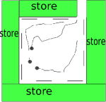
(a) A testing environment: in the encircled space, only one exit exists, but the mobile robot can only observe the space within the dashed lines, and it has to observe the motions of cars, shown as black dots in the figure, to estimate the location of the exit.

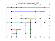
(b) Example trajectories in Gridworld MDP: each agent starts from a random position, and follows an optimal policy to approach the exit. The black dots represent the initial positions of the agents. Each colored path denotes one trajectory with finite length.

Figure 1: A simulated environment

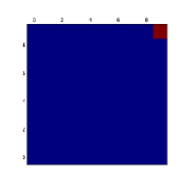
(a) A reward table for the gridworld mdp on a $10\times 10$ grid.

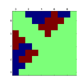
(b) An example of a reward table for one objectworld mdp on a $10\times 10$ grid: it depends on randomly placed objects.

Figure 2: Examples of true reward tables

The second environment is an objectworld mdp [9]. It is similar to the gridworld mdp, but with a set of objects randomly placed on the grid. Each object has an inner color and an outer color, selected from a set of possible colors, $C$. The reward of a state is positive if it is within 3 cells of outer color $C1$ and 2 cells of outer color $C2$, negative if it is within 3 cells of outer color $C1$, and zero otherwise. Other colors are irrelevant to the ground truth reward. One example is shown in Figure 2b. In this work, we place two random objects on the grid, and use a linear function to represent the reward, where the feature of a state indicates its discrete distance to each inter color and outer color in $C$. The true reward is nonlinear.

In each environment, the robot’s trajectories are generated based on the true reward function.

V-A Qualitative Results

We show some qualitative results with the proposed methods on 50 randomly generated trajectories, where each trajectory has a random start and 10 steps.

For the p-norm approximation, we manually choose several parameter settings. In each of the parameter settings, we run the algorithm fifty times with random reward parameter initializations, and compare their log-likelihood values. For the parameter leading to the highest log-likelihood, we compute the reward table. Several comparisons of ground-truth rewards and learned rewards are shown in Figures 3a and 4a. For the g-soft approximation, we follow the same procedure, and the results are shown in Figures 3b and 4b.

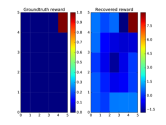
(a) Demonstration of the p-norm method on a gridworld mdp: $k=100,b=1,e=1000,\alpha=0.01$. Left: ground truth. Right: recovered reward functin.

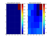
(b) Demonstration of the g-soft method on a gridworld mdp: $k=10,b=1,e=1000,\alpha=0.01$.Left: ground truth. Right: recovered rewrad function.

Figure 3: Reward learning on gridworld mdp

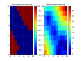
(a) Demonstration of the p-norm method on an objectworld mdp: $k=30,b=1,e=1000,\alpha=0.01$. Left: ground truth. Right: recovered reward function.

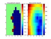
(b) Demonstration of the g-soft method on an objectworld mdp: $k=0.5,b=1,e=1000,\alpha=0.01$. Left: ground truth. Right: recovered reward function.

Figure 4: Reward learning on objectworld mdp

V-B Quantitative Results

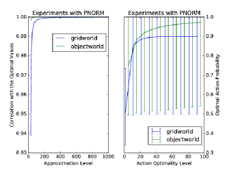
Figure 5: The effect of different approximation levels $k$ and confidence level $b$ on optimal value and optimal action selection with p-norm approximation: in both environments, when $k>500$, the approximated value function is nearly identical to the optimal value. For $b$, the probability to choose the optimal action keeps increasing in objectworld, but remains smaller than 0.9 in grid world.

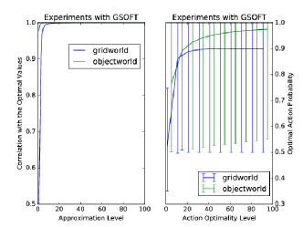
Figure 6: The effect of different approximation levels $k$ and confidence level $b$ on optimal value and optimal action selection with g-soft approximation: in both environments, when $k>20$, the approximated value function is nearly identical to the optimal value. For $b$, the probability to choose the optimal action keeps increasing in objectworld, but remains smaller than 0.9 in grid world.

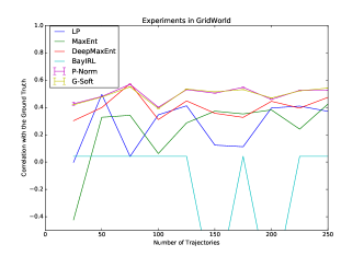
Figure 7: Comparison in gridworld: for each set of trajectories, we run the proposed method 100 times, each time with a random initial parameter, and compute the correlation coefficient between the learned reward and the true reward. The correlation coefficients for linear programming (LP), maximum entropy (MaxEnt), Bayesian IRL(BayIRL), and deep learning (DeepMaxEnt) are plotted. For the proposed method (PNORM approximation and GSOFT approximation), the correlation coefficient of the reward function with the highest log-likelihood and the standard deviation of the coefficients under random initial parameters are plotted.

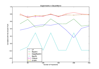
Figure 8: Comparison in objectworld: for each set of trajectories, we run the proposed method 100 times, each time with a random initial parameter, and compute the correlation coefficient between the learned reward and the true reward. The correlation coefficients for linear programming (LP), maximum entropy (MaxEnt), Bayesian IRL(BayIRL), and deep learning (DeepMaxEnt) are plotted. For the proposed method (PNORM approximation and GSOFT approximation), the correlation coefficient of the reward function with the highest log-likelihood and the standard deviation of the coefficients under random initial parameters are plotted.

We evaluate the proposed method in three aspects: the accuracy of the value function approximation, a comparison of the proposed method with existing methods, and the scalability of the proposed method to large state space. We change the two environments to $5\times 5$ grids to reduce the computation time, but the dimension of the feature vector is still high enough to make the reward function complex. The manually selected parameters for reward learning are the number of iterations $e=1000$, the learning rate $\alpha=0.001$, and the discount factor $\gamma=0.9$. The parameters to be evaluated include the approximation level $k$ and the confidence level $b$.

First, we run the approximate value iteration algorithm and the motion model in Equation (6) with different values of $k$ and $b$ in two environments. To evaluate the approximation level $k$, we set the range of $k$ as 30 to 1000 for p-norm approximation, and 1 to 100 for g-soft approximation, and set $b=1$. For each $k$, we compute the approximate value function and evaluate it based on the correlation coefficient between the approximate value function and the optimal value function. To evaluate the confidence level $b$, we choose the range of $b$ as 1 to 100 for both approximations, and $k=1000$ for p-norm approximation, $k=100$ for g-soft approximation. For each $b$, we compute the Q-function and the probability to take the optimal action in each state. With only $5\times 5$ states, we compute the exact minimum, maximum, and mean value of the probabilities in all states to take the optimal actions. The results are shown in Figures 5 and 6.

The figures show that with sufficiently large $k$, the approximate value iteration generates almost the identical result as the exact calculation. Therefore, to compute the gradient of the optimal value with respect to a reward parameter, we can choose the largest $k$ that does not lead to data overflow. However, the situation is different for $b$. Although the mean probability of optimal actions increases with larger $b$, the mean value of the probabilities in all states to take the optimal actions is always smaller than 0.9 in gridworld, because many state-action pairs have the same Q-values, leading to multiple optimal policies, and the probability for each policy is always smaller than 1.

Second, we compare the proposed method with existing methods, including the linear programming (LP) approach in [5], Bayesian method (BayIRL) in [4], the maximum entropy (MaxEnt) approach in [2], and a latest method based on deeep learning (DeepMaxEnt) in [13]. We randomly generate different numbers of trajectories, ranging from 25 trajectories to 250 trajectories, and run the proposed method 100 times on the data, each with a random initial parameter. The learned rewards are evaluated based on the correlation coefficient with the true reward function. For existing methods, we compute the correlation coefficient, and for the proposed method, we compute the correlation coefficient of the reward function associated with the highest log-likelihood. To evaluate the multi-start strategy, we also plot the standard deviation of the correlation coefficients. The parameter for p-norm approximation is $k=100,b=1$ in both environments, and the parameter for g-soft approximation is $k=10,b=1$ in both environments. Other parameters are shared among all methods. The comparison results are plotted in Figures 7 and 8.

The results show that in gridworld, where the ground truth is a linear reward function, the proposed method performs better than existing methods, and only DeepMaxent outperforms the proposed method occasionally. In objectworld, where the ground truth is a non-linear reward function, the proposed method is second to DeepMaxent, because it adopts a non-linear neural network to model the reward function while the proposed method uses a linear function. Besides, the theoretically locally optimal results are quite similar to each other, because under a linear reward function and a large approximate level $k$, the approximated Q values are approximately linear and the objective function is close to a convex function.

Third, we test the scalability of the proposed method. We change the number of states in the objectworld environment, and test the amount of time needed for one iteration of gradient ascent. To record the accurate time, we do not adopt any parallel computing, and run the proposed method on a single core of Intel CPU i7-6700. The implementation is a mix of C and python. The result is given in Table I.

TABLE I: Computation time (second) for one iteration of gradient ascent.

state size	25	100	400	1600	6400	14400
pnorm	0.007	0.112	2.570	58.588	1560.014	8689.786
gsoft	0.004	0.093	2.088	54.136	1398.481	7035.641

The result shows that the algorithm can run a fair number of states, and in practice, the method can be easily implemented as an efficient parallel algorithm by converting the Bellman Gradient Iteration into matrix operations. Another bottleneck of the method is fitting the transition model into the memory, whose size is $O(N_{S}^{2}*N_{A})$, but in practice, we may divide it into sub-matrices for efficiency

In summary, with a proper motion model to describe the actions, the proposed method performs better than existing methods under linear reward functions while comparable to the state-of-the-art method based on deep neural network. Besides, the proposed method is defined on state-action pairs, instead of trajectories of fixed length, and this provides great flexibility in modeling practical actions.

Two minor drawbacks of the proposed methods are the locally optimal results and the resource-intensive computation in large state space. But in practice, an approximately global optimum can be achieved with a sufficiently high approximation level. The computation problem can be solved with parallel computing on multi-core CPU or GPU. The major drawback of the proposed method is the assumption of a known environment dynamics. The problem may be solved by sampling the motion trajectories and estimating the dynamics.

VI Conclusions

This work introduced two approximations of the Bellman Optimality Equation to model the relation between action selection and reward function in a differentiable way, and proposed a Bellman Gradient Iteration method to efficiently compute the gradient of Q-value with respect to reward functions. This method allows us to learn the reward with gradient methods and model different behaviors by varying the approximation level. We test the proposed method in two simulated environments, and reveal how different parameter settings affect the accuracy of reward learning. We compare the proposed method with existing approaches, and show that the proposed method is more accurate and flexible in learning reward functions from the observed actions

In future work, we will extend the proposed framework in multiple directions. First, we will search for other approximation methods that lead to a concave Q-function, thus a global optimum can be found. Second, we will apply the proposed method to other scenarios with different motion models, like online learning for human motion analysis and deep learning for nonlinear reward functions.

References

- [1] B. D. Argall, S. Chernova, M. Veloso, and B. Browning, “A survey of robot learning from demonstration,” Robotics and Autonomous Systems, vol. 57, no. 5, pp. 469 – 483, 2009.
- [2] B. D. Ziebart, A. Maas, J. A. Bagnell, and A. K. Dey, “Maximum entropy inverse reinforcement learning,” in Proc. AAAI, 2008, pp. 1433–1438.
- [3] P. Abbeel and A. Y. Ng, “Apprenticeship learning via inverse reinforcement learning,” in Proceedings of the twenty-first international conference on Machine learning. ACM, 2004, p. 1.
- [4] D. Ramachandran and E. Amir, “Bayesian inverse reinforcement learning,” in Proceedings of the 20th International Joint Conference on Artifical Intelligence, ser. IJCAI’07. San Francisco, CA, USA: Morgan Kaufmann Publishers Inc., 2007, pp. 2586–2591.
- [5] A. Y. Ng and S. Russell, “Algorithms for inverse reinforcement learning,” in in Proc. 17th International Conf. on Machine Learning, 2000.
- [6] N. D. Ratliff, J. A. Bagnell, and M. A. Zinkevich, “Maximum margin planning,” in Proceedings of the 23rd international conference on Machine learning. ACM, 2006, pp. 729–736.
- [7] G. Neu and C. Szepesvári, “Apprenticeship learning using inverse reinforcement learning and gradient methods,” UAI, 2007.
- [8] Q. P. Nguyen, B. K. H. Low, and P. Jaillet, “Inverse reinforcement learning with locally consistent reward functions,” in Advances in Neural Information Processing Systems, 2015, pp. 1747–1755.
- [9] S. Levine, Z. Popovic, and V. Koltun, “Nonlinear inverse reinforcement learning with gaussian processes,” in Advances in Neural Information Processing Systems 24, J. Shawe-Taylor, R. S. Zemel, P. L. Bartlett, F. Pereira, and K. Q. Weinberger, Eds. Curran Associates, Inc., 2011, pp. 19–27.
- [10] C. Finn, S. Levine, and P. Abbeel, “Guided cost learning: Deep inverse optimal control via policy optimization,” in Proceedings of the 33rd International Conference on Machine Learning, vol. 48, 2016.
- [11] J. Choi and K.-E. Kim, “Inverse reinforcement learning in partially observable environments,” Journal of Machine Learning Research, vol. 12, no. Mar, pp. 691–730, 2011.
- [12] S. Levine and V. Koltun, “Continuous inverse optimal control with locally optimal examples,” in ICML ’12: Proceedings of the 29th International Conference on Machine Learning, 2012.
- [13] M. Wulfmeier, P. Ondruska, and I. Posner, “Deep inverse reinforcement learning,” CoRR, 2015.
- [14] K. Mombaur, A. Truong, and J.-P. Laumond, “From human to humanoid locomotion—an inverse optimal control approach,” Autonomous robots, vol. 28, no. 3, pp. 369–383, 2010.
- [15] C. Dimitrakakis and C. A. Rothkopf, “Bayesian multitask inverse reinforcement learning,” in European Workshop on Reinforcement Learning. Springer, 2011, pp. 273–284.
- [16] J. Choi and K.-E. Kim, “Nonparametric bayesian inverse reinforcement learning for multiple reward functions,” in Advances in Neural Information Processing Systems, 2012, pp. 305–313.
- [17] R. S. Sutton and A. G. Barto, Reinforcement learning: An introduction. MIT press Cambridge, 1998, vol. 1, no. 1.