Origins of anisotropic thermal expansion in flexible materials

Abstract

A definition of the Grüneisen parameters for anisotropic materials is derived based on the response of phonon frequencies to uniaxial stress perturbations. This Grüneisen model relates the thermal expansion in a given direction ($\alpha_{ii}$) to one element of the elastic compliance tensor, which corresponds to the Young’s modulus in that direction ($Y_{ii}$). The model is tested through ab initio prediction of thermal expansion in zinc, graphite, and calcite using density functional perturbation theory, indicating that it could lead to increased accuracy for structurally complex systems. The direct dependence of $\alpha_{ii}$ on $Y_{ii}$ suggests that materials which are flexible along their principal axes but rigid in other directions will generally display both positive and negative thermal expansion.

I Introduction

Materials which lack cubic symmetry will expand (or contract) at different rates in different directions in response to a change in temperature. Thermal expansion anisotropy has been the subject of considerable recent attention due to the discovery of flexible framework materials with unusually large positive or negative coefficients of thermal expansion (CTEs) along one or two crystal axes. Goodwin et al. (2008, 2009); Nanthamathee et al. (2014); Cai and Katrusiak (2014); Takenaka et al. (2017); Dove and Fang (2016) However, anisotropy has a long history of complicating fundamental understanding of the origins of thermal expansion, Kopp (1852) and, owing to the thermal stress introduced in consolidated polycrystals, anisotropy can limit the practical uses of materials. Cheng et al. (1998); Romao et al. (2016)

In some cases the origin of thermal expansion anisotropy can be appreciated intuitively by inspection of the structure: the interatomic interactions in graphite are obviously stronger within the graphene layers than between them. In other cases the relationship is more subtle, e.g., temperature-induced displacive phase transitions in quartz and cristobalite introduce significant thermal expansion anisotropy while retaining the network topology.(Barron et al., 1982; Schmahl et al., 1992) The orthorhombic Sc₂W₃O₁₂ structure, which produces characteristically large anisotropy between axes with negative and positive CTEs, is isomorphic to the cubic aluminosilicate framework of garnet. Romao et al. (2016); Evans et al. (1998) In the metal-organic wine-rack framework material MIL-53 replacement of an OH^- anion by F^- leaves the crystallographic symmetry unchanged but significantly modifies the thermal expansion anisotropy, changing the volumetric CTE ($\alpha_{V}$) from positive to negative. (Nanthamathee et al., 2014)

The origins of thermal expansion in crystalline solids are commonly studied through a model originated by Grüneisen Grüneisen (1912) which relates the contribution of a phonon to the thermal expansion to the volume derivative of its frequency. The Grüneisen approach is useful because changes in phonon frequencies as a function of volume can be measured using variable-pressure inelastic scattering techniques and calculated ab initio using, for example, density-functional perturbation theory (DFPT), allowing explication of the mechanisms of thermal expansion. (Mittal et al., 2001; Zwanziger, 2007; Zhou et al., 2008; Peterson et al., 2010; Yoon et al., 2011; Rimmer et al., 2014a, b) However, this model does not consider material anisotropy and an extension, incorporating coupling between elastic anisotropy and thermal expansion anisotropy, is required for non-cubic crystal families.

The most notable such extension, based on replacing the volume perturbation by uniaxial strain perturbations, was developed by Barron and Munn Barron and Munn (1967) following Grüneisen’s approach. Grüneisen and Goens (1924) Due to the experimental challenges involved in applying uniaxial strain to a sample, (Jones and Dunstan, 1996) the anisotropic Grüneisen theory of Ref. 21 has until recently been used primarily to calculate directional Grüneisen parameters from experimental thermal expansion and heat capacity data, (Bailey and Yates, 1970; Yates et al., 1975; Sears et al., 1979; Barron et al., 1982; Huang et al., 2016; Romao et al., 2016) and to identify the contributions of acoustic modes to thermal expansion anisotropy. (Ramachandran and Srinivasan, 1972) Therefore, until the fairly recent development of ab initio methods which could calculate phonon band structures as a function of an arbitrary strain, the ability of the Barron–Munn model to predict anisotropic thermal expansion had been untested. Ab initio prediction of thermal expansion anisotropy has shown results mixed between qualitative and quantitative levels of accuracy. (Fang et al., 2014; Arnaud et al., 2016; Wang et al., 2016; Murshed et al., 2016; Liu et al., 2017)

In order to understand and predict the behaviour of flexible materials, defined here as those with some elastically compliant direction, we must understand how thermal expansion and elasticity are coupled. To further this goal, herein a Grüneisen model based on uniaxial stress perturbations is reported, which allows an explicit treatment of the coupling between Grüneisen parameters along different axes. The ability of the uniaxial stress model to predict axial CTEs is compared to that of the uniaxial strain model through DFPT calculations on several simple highly anisotropic materials (Fig. 1).

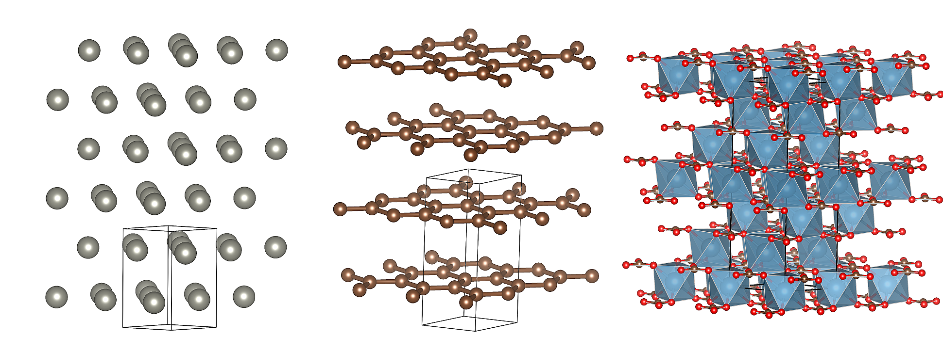
Figure 1: Crystal structures of materials with highly anisotropic thermal expansion and elastic properties used herein to test anisotropic Grüneisen models. ics From left to right: zinc, graphite, calcite. The $c$ axes are aligned vertically.

II Grüneisen Models

II.1 The Isotropic Grüneisen Model

To understand the place of anisotropy within the Grüneisen formalism, it is instructive to begin with a brief discussion of the original Grüneisen model for isotropic or cubic systems. The thermodynamic Grüneisen parameter ($\gamma$) is introduced through the identity

$$\alpha_{V}=\frac{1}{V}\left(\frac{\partial V}{\partial{T}}\right)_{P}=\frac{1}{K_{T}}\left(\frac{\partial S}{\partial{V}}\right)_{T}=\frac{1}{V}\frac{\gamma C_{V}}{K_{T}},$$ (1)

where the quantity $\gamma C_{V}$ represents a ‘phonon pressure’, resulting from vibrational anharmonicity, which acts against the bulk modulus ($K_{T}$) to change the dimensions of the unit cell. Using the quasiharmonic approximation (QHA), the contribution of an individual phonon mode with frequency $\omega_{n,\mathbf{k}}$ to the thermal expansion is determined through the mode Grüneisen parameter ($\gamma_{n,\mathbf{k}}$), where

$$\gamma_{n,\mathbf{k}}=-\frac{V}{\omega_{n,\mathbf{k}}}\left(\frac{\partial\omega_{n,\mathbf{k}}}{\partial V}\right)_{T}.$$ (2)

Then, $\gamma$ and $\gamma_{n,\mathbf{k}}$ are related by

$$\gamma=\frac{\sum_{n,\mathbf{k}}\gamma_{n,\mathbf{k}}C_{V,n,\mathbf{k}}}{\sum_{n,\mathbf{k}}C_{V,n,\mathbf{k}}}.$$ (3)

Differences between $\gamma$ as defined by Eq. (1) and $\gamma$ as defined by Eq. (3) are due to anharmonic phonon-phonon interactions, and therefore are reduced with decreasing temperature. (Fultz, 2010) The exact validity of Eqs. (1–3) also requires elastic isotropy of the lattice vectors and internal strain coordinates. (Hofmeister and Mao, 2002) When cubic symmetry is not present, the phonon frequencies do not depend only on the volume of the system, but also on the combination of strains required to reach a given volume from the equilibrium state.

II.2 Uniaxial Strain Models

Barron and Munn defined Grüneisen parameters for the response of a phonon to a (uniaxial) Lagrangian strain ($\eta_{ij}$) as: (Barron and Munn, 1967)

$$\hat{\gamma}_{ij,n,\mathbf{k}}=-\frac{1}{\omega_{n,\mathbf{k}}}\left(\frac{\partial\omega_{n,\mathbf{k}}}{\partial\eta_{ij}}\right)_{\eta_{kl\neq ij}}.$$ (4)

Following averaging, by analogy to Eq. (3) the directional thermal expansion is then constructed as: (Barron and Munn, 1967)

$$\alpha_{ij}=\left(\frac{\partial\eta_{ij}}{\partial T}\right)_{\bm{t}}=\frac{C_{\bm{\eta}}}{V}\sum_{kl}s_{ijkl}\hat{\gamma}_{ij},$$ (5)

where $s_{ijkl}$ are elements of the isothermal compliance tensor. Note that the directional thermal expansion is defined here as a derivative under conditions of constant ‘thermodynamic tension’ ($\bm{t}$), where

$$t_{ij}=\left(\frac{\partial F}{\partial\eta_{ij}}\right)_{\eta_{kl\neq ij},T}.$$ (6)

Therefore, the perturbation in Eq. (4) is uniaxial in terms of strain and thermodynamic tension, but not stress, since there are generally stresses in the directions perpendicular to $ij$ induced by the Poisson effect. These transverse stresses are accounted for in Eq. (5) by linking the directional Grüneisen parameters through the cross-compliances, which assumes a mechanical coupling between the axial CTEs.

Choy et al. (Choy et al., 1984) treated Barron and Munn’s definition of the Grüneisen parameter as arbitrary, and instead assumed an expression intermediate between Eq. (1) and Eq. (5):

$$\alpha_{ij}=\frac{1}{V}\frac{\tilde{\gamma}_{ij}C_{\bm{\eta}}}{3K_{T}}.$$ (7)

However, this model is necessarily limited by its neglect of elastic anisotropy, and has been used sparingly for ab initio prediction of thermal expansion. (Wdowik et al., 2011)

II.3 Uniaxial Stress Model

The derivation of a Grüneisen model based on uniaxial stress perturbations begins by considering the thermal expansion of a volume ($V$) under a constant stress ($\bm{\sigma}$). This stress is treated as a Cauchy stress, i.e., the volume of the stress-free reference state ($V_{0}$) is approximately equal to $V$. Accordingly, the conjugate infinitesimal strain ($\bm{e}$) is used, leading to the definition of thermal expansion used experimentally in the limit of small strains. Then, an arbitrary element of the thermal expansion tensor ($\bm{\alpha}$) is related to an uniaxial stress perturbation as

$$\alpha_{ij} =\left(\frac{\partial e_{ij}}{\partial T}\right)_{\bm{\sigma}}=\left(\frac{\partial e_{ij}}{\partial\sigma_{ij}}\right)_{T,\sigma^{\prime}}\left(\frac{\partial\sigma_{ij}}{\partial T}\right)_{e_{ij},\sigma^{\prime}}=s_{ijij}\left(\frac{\partial\sigma_{ij}}{\partial T}\right)_{e_{ij},\sigma^{\prime}},$$ (8)

where the subscript $\sigma^{\prime}$ indicates that the elements of $\bm{\sigma}$ other than $\sigma_{ij}$ are kept constant. The relationship between $\sigma_{ij}$ and the free energy is then considered:

$$\left(\frac{\partial F}{\partial e_{ij}}\right)_{T,\sigma^{\prime}} =-\frac{V_{0}}{2}\left(\frac{\partial\left(\bm{\sigma}:\bm{e}\right)}{\partial e_{ij}}\right)_{T,\sigma^{\prime}}$$ (9a)

$$=-V_{0}\left(\sigma_{ij}+\frac{1}{2}\sum_{kl\neq ij}\sigma_{kl}\left(\frac{\partial e_{kl}}{\partial e_{ij}}\right)_{T,\sigma^{\prime}}\right)$$ (9b)

$$\sigma_{ij}=-\frac{1}{V_{0}}\left(\frac{\partial F}{\partial e_{ij}}\right)_{T,\sigma^{\prime}}+\frac{1}{2}\sum_{kl\neq ij}\sigma_{kl}\nu_{ijkl}.$$ (10)

By substitution,

$$\alpha_{ij}=s_{ijij}\frac{\partial}{\partial T}\left(-\frac{1}{V_{0}}\left(\frac{\partial F}{\partial e_{ij}}\right)_{T,\sigma^{\prime}}+\frac{1}{2}\sum_{kl\neq ij}\sigma_{kl}\nu_{ijkl}\right)_{e_{ij},\sigma^{\prime}},$$ (11)

and, using the QHA,

$$\alpha_{ij}=-s_{ijij}\left(\sum_{n,\mathbf{k}}\frac{\hbar}{V_{0}}\left(\frac{\partial\omega_{n,\mathbf{k}}}{\partial e_{ij}}\right)_{T,\sigma^{\prime}}\left(\frac{\partial}{\partial T}\frac{1}{e^{k_{\text{B}}T\omega_{n,\mathbf{k}}}-1}\right)_{e_{ij},\sigma^{\prime}}-\frac{1}{2}\sum_{kl\neq ij}\sigma_{kl}\frac{\partial\nu_{ijkl}}{\partial T}\right).$$ (12)

At this point $C_{\sigma^{\prime}}$, the heat capacity under conditions of constant strain along $ij$ and constant stress along $kl\neq ij$, is introduced:

$$C_{\sigma^{\prime}}=T\left(\frac{\partial S}{\partial T}\right)_{e_{ij},\sigma^{\prime}}=\sum_{n,\mathbf{k}}C_{\sigma^{\prime},n,\mathbf{k}}=\sum_{n,\mathbf{k}}\hbar\omega_{n,\mathbf{k}}\left(\frac{\partial}{\partial T}\frac{1}{e^{k_{\text{B}}T\omega_{n,\mathbf{k}}}-1}\right)_{e_{ij},\sigma^{\prime}}.$$ (13)

This heat capacity can be compared to $C_{\bm{e}}$ as follows:

$$C_{\sigma^{\prime}} =T\left(\frac{\partial S}{\partial T}\right)_{\bm{e}}+T\sum_{kl\neq ij}\left(\frac{\partial S}{\partial e_{kl}}\right)_{T,\sigma_{mn\neq kl}}\left(\frac{\partial e_{kl}}{\partial T}\right)_{\bm{\sigma}}$$ (14a)

$$=C_{\bm{e}}+{T}{V_{0}}\sum_{kl\neq ij}\left(\left(\frac{\partial\sigma_{kl}}{\partial T}\right)_{e_{kl},\sigma_{mn\neq kl}}-\frac{1}{2}\sum_{mn\neq kl}\sigma_{mn}\frac{\partial\nu_{klmn}}{\partial T}\right)\alpha_{kl}$$ (14b)

$$=C_{\bm{e}}+{T}{V_{0}}\sum_{kl\neq ij}\left(\frac{\alpha_{kl}}{s_{klkl}}-\frac{1}{2}\sum_{mn\neq kl}\sigma_{mn}\frac{\partial\nu_{klmn}}{\partial T}\right)\alpha_{kl},$$ (14c)

making use of Eqs. (8) and (9). Then, the Grüneisen parameters are defined:

$$\check{\gamma}_{ij,n,\mathbf{k}} =-\frac{1}{\omega_{n,\mathbf{k}}}\left(\frac{\partial\omega_{n,\mathbf{k}}}{\partial e_{ij}}\right)_{T,\sigma^{\prime}}=-\frac{1}{s_{ijij}}\left(\frac{\partial~{}\text{ln}~{}\omega_{n,\mathbf{k}}}{\partial\sigma_{ij}}\right)_{T,\sigma^{\prime}}$$ (15)

$$\check{\gamma}_{ij} =\frac{\sum_{n,\mathbf{k}}\check{\gamma}_{ij,n,\mathbf{k}}C_{\sigma^{\prime},n,\mathbf{k}}}{\sum_{n,\mathbf{k}}C_{\sigma^{\prime},n,\mathbf{k}}},$$ (16)

leading to the following expression for $\alpha_{ij}$

$$\alpha_{ij}=s_{ijij}\left(\check{\gamma}_{ij}\frac{C_{\sigma^{\prime}}}{V_{0}}+\frac{1}{2}\sum_{kl\neq ij}\sigma_{kl}\frac{\partial\nu_{ijkl}}{\partial T}\right).$$ (17)

By assuming that the external stress or the temperature derivatives of the transverse Poisson ratios are negligible, and that $C_{\sigma^{\prime}}\approx C_{\bm{e}}$, the simplified expression

$$\alpha_{ij}=s_{ijij}\check{\gamma}_{ij}\frac{C_{\bm{e}}}{V_{0}}$$ (18)

is obtained. For tetragonal and hexagonal crystal families, it is desirable to consider a biaxial stress perturbation along $a$ and $b$ in order to preserve phonon degeneracies. (Gan and Liu, 2016) Therefore, analogous areal versions of Eqs. (15), (17), and (18) are required:

$$\check{\gamma}_{A,n,\mathbf{k}} =-\left(\frac{\partial~{}\text{ln}~{}\omega_{n,\mathbf{k}}}{\partial~{}\text{ln}~{}A}\right)_{T,\sigma_{cc}}$$ (19)

$$\alpha_{aa} =\left(s_{aaaa}+s_{aabb}\right)\left(\check{\gamma}_{A}\frac{C_{\sigma_{cc}}}{V_{0}}+\frac{1}{2}\sigma_{cc}\frac{\partial\nu_{aacc}}{\partial T}\right)$$ (20)

$$\alpha_{aa} =\left(s_{aaaa}+s_{aabb}\right)\check{\gamma}_{A}\frac{C_{\bm{e}}}{V_{0}},$$ (21)

where $A$ is the area of the $ab$ plane.

III Computational Methods

In order to test the uniaxial stress model in comparison to the uniaxial strain model, the axial CTEs of several materials were calculated ab initio using both models. The selected materials (graphite, zinc, and calcite (Fig. 1)) exemplify simple structures with highly anisotropic thermal and mechanical behaviour and their physical properties are well-known. (Bailey and Yates, 1970; Gauster and Fritz, 1974; Meyerhoff and Smith, 1962; Ledbetter, 1977; Ramachandran and Srinivasan, 1972; Rao et al., 1968; Chen et al., 2001; Dandekar and Ruoff, 1968)

Density functional theory calculations were carried out with the Abinit software package (v. 8.0.8) using pseudopotentials and plane-waves. (Gonze et al., 2016; Bottin et al., 2008) All calculations were performed using the Perdew–Burke–Ernzerhof generalized gradient approximation to the exchange–correlation functional; (Perdew et al., 1996) for graphite and calcite the vdw–DFT–D2 dispersion correction was added. (Grimme, 2006) Optimized norm-conserving Vanderbilt pseudopotentials (Hamann, 2013) from the Abinit library abi were used in all cases; these pseudopotentials were tested by comparison of calculated elastic properties to experimental results. si Plane-wave basis set energy cutoffs, Monkhorst–Pack grid spacings, (Monkhorst and Pack, 1976) and van der Waals tolerance factors (Grimme, 2006) were chosen through convergence studies.si The values of these parameters can be found in tabular form in the Supplemental Material. si

For each material, the structure was relaxed under conditions of zero external stress, and under uniaxial (biaxial) stress and strain perturbations along the $c$ axis ($ab$ plane). The magnitudes of the perturbations were generally chosen to give strains of 0.1% for both the stress and strain cases. The phonon energies and elastic tensors of the relaxed geometries were calculated using DFPT; (Gonze, 1997; Gonze and Lee, 1997; Van Troeye et al., 2016) integration of phonon energies over the Brillouin zone yielded heat capacities. (Lee and Gonze, 1995) Grüneisen parameters and axial CTEs were obtained from these data as described above. In the case of zinc, electronic contributions to the axial CTEs were included. (Barron and Munn, 1967; Verstraete and Gonze, 2001)

IV Results

The first two materials considered, zinc and graphite, have very simple structures and similar thermoelastic properties. The stress and strain models used to predict their axial thermal expansion showed reasonable agreement with experimental data (Fig. 2). The predicted $\alpha_{cc}$ in graphite was significantly lower than the experimental value at low temperature, despite the calculated phonon band structure and elastic tensor providing good matches to experiment (see Supplemental Material). si However, the van der Waals nature of the interactions along $c$ provides a significant challenge for dispersion-corrected DFT. (Van Troeye et al., 2016; Lechner et al., 2016) Otherwise, the stress model of (Eq. (18)) produced identical results to that of the strain model (Eq. (5)).

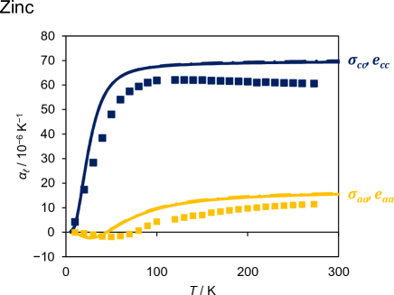
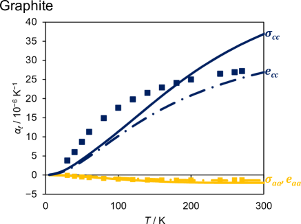
Figure 2: Linear thermal expansion in zinc and graphite along the $a$ (orange lines) and $c$ (blue lines) axes, as predicted by stress (solid lines) and strain (dashed lines) models. Experimental data (Bailey and Yates, 1970; Meyerhoff and Smith, 1962) are shown as squares.

Zinc and graphite have significant elastic anisotropy, as their $c$ axes are considerably more compliant than their $a$ axes, (si, ; Ledbetter, 1977; Gauster and Fritz, 1974) but the elastic couplings between the $a$ and $c$ axes are not unusually strong. (for zinc $\nu_{aacc}=0.32$ and $\nu_{ccaa}=0.13$; for graphite $\nu_{aacc}=-0.20$ and $\nu_{ccaa}=-0.008$). Since the stress and strain perturbations are identical in the limit of zero Poisson ratio, a more rigorous test can be obtained by considering a material with strong elastic couplings between axes. The calculated elastic tensor of calcite indicates that it has significant elastic couplings between its principal axes (Fig. 3). The directional Young’s moduli ($Y_{ii}={s_{iiii}}^{-1}$) also show significant anisotropy (Fig. 3), and therefore the elastic contribution to thermal expansion anisotropy in calcite is expected to be different from those of zinc and graphite.

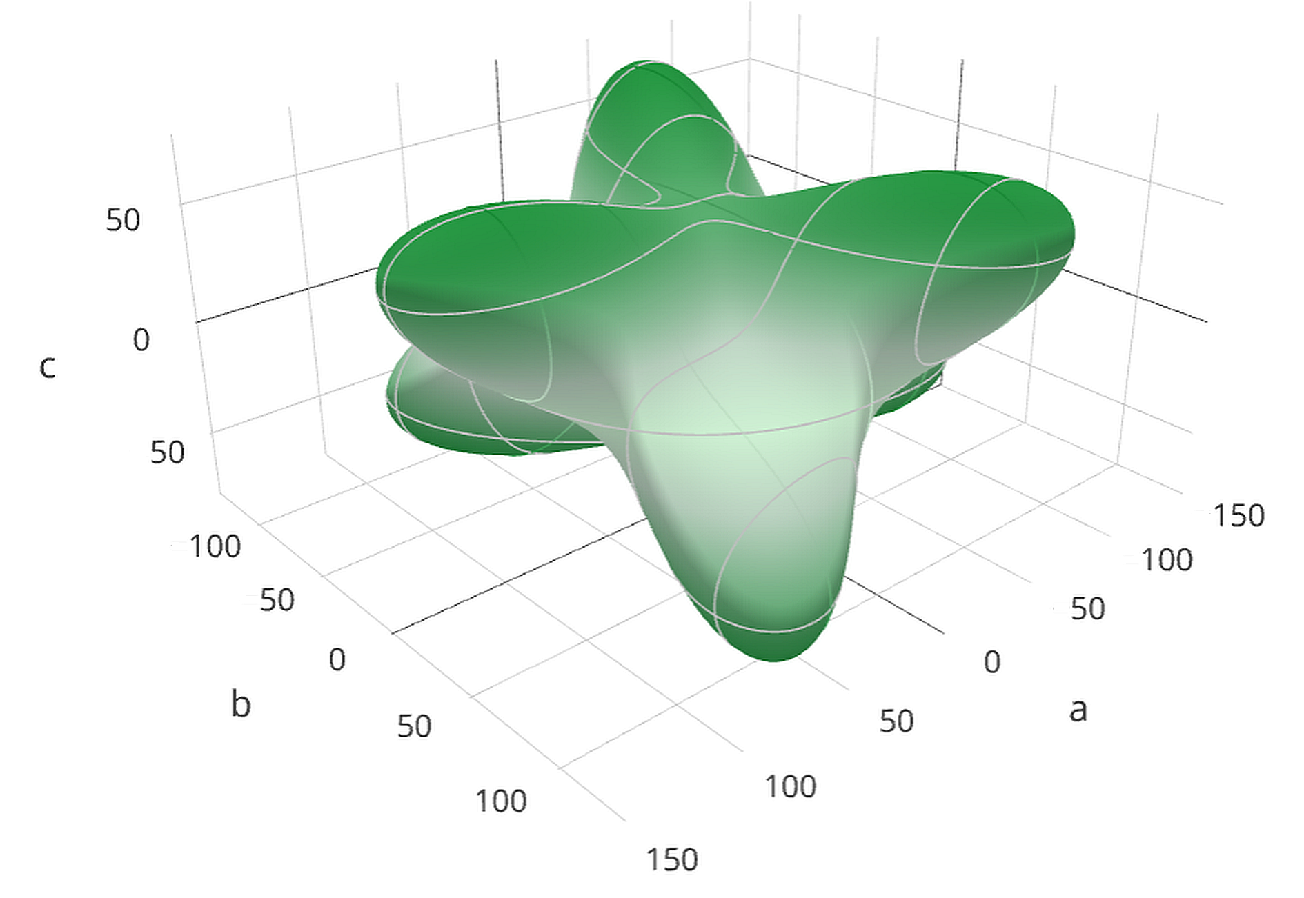
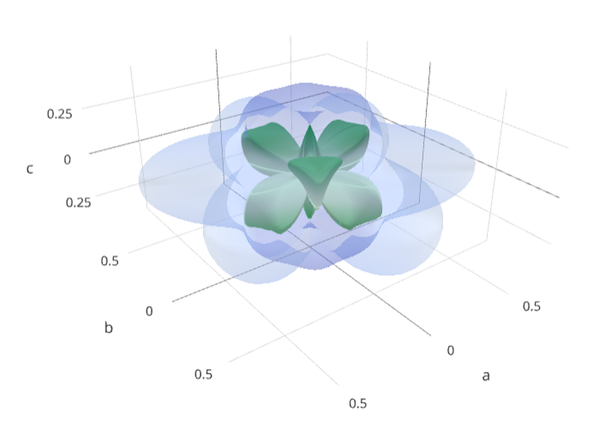
Figure 3: Directional Young’s moduli (in GPa, left) and Poisson ratios (right) of calcite. The Young’s modulus in a given direction is shown as a green surface. The surface corresponding to the maximum Poisson ratio is shown in blue, and the surface corresponding to the minimum Poisson ratio is shown in green. Visualization generated with ELATE. ela ; Gaillac et al. (2016)

Unlike in the cases of zinc and graphite, the stress and strain models gave significantly different predictions of axial thermal expansion in calcite (Fig. 4); with the stress model providing a good match to the experimental data and the strain model erroneously predicting $\alpha_{aa}$ to be positive and $\alpha_{cc}$ to be negative. Thermal expansion anisotropy in calcite is driven by low-energy acoustic and optic modes (Fig. 5) in which the CO${}_{3}^{2-}$ unit remains rigid. The acoustic modes which propagate along $c$ (with wavevector $\Gamma$–Z) have large positive Grüneisen parameters with respect to all perturbations, while those which propagate in the $ab$ plane have negative Grüneisen parameters. The group of optic modes with negative mode Grüneisen parameters below 150 cm^-1 involves librations of the CO${}_{3}^{2-}$ unit, while the group between 150 and 450 cm^-1 includes motion of the Ca²⁺ ion, although there is considerable eigenvector mixing away from $\Gamma$.si This view of calcite as, in some respects, a framework solid, is supported by the directional Young’s moduli showing maxima coinciding with the directions of Ca–O–C linkages and by the large Poisson ratios in these directions (Fig. 3).

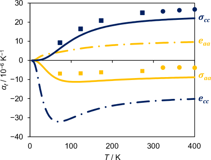
Figure 4: Linear thermal expansion in calcite along the $a$ (orange lines) and $c$ (blue lines) axes, as predicted by stress (solid lines) and strain (dashed lines) models. Experimental data are shown as squares (Ref. 28) and circles (Ref. 43).

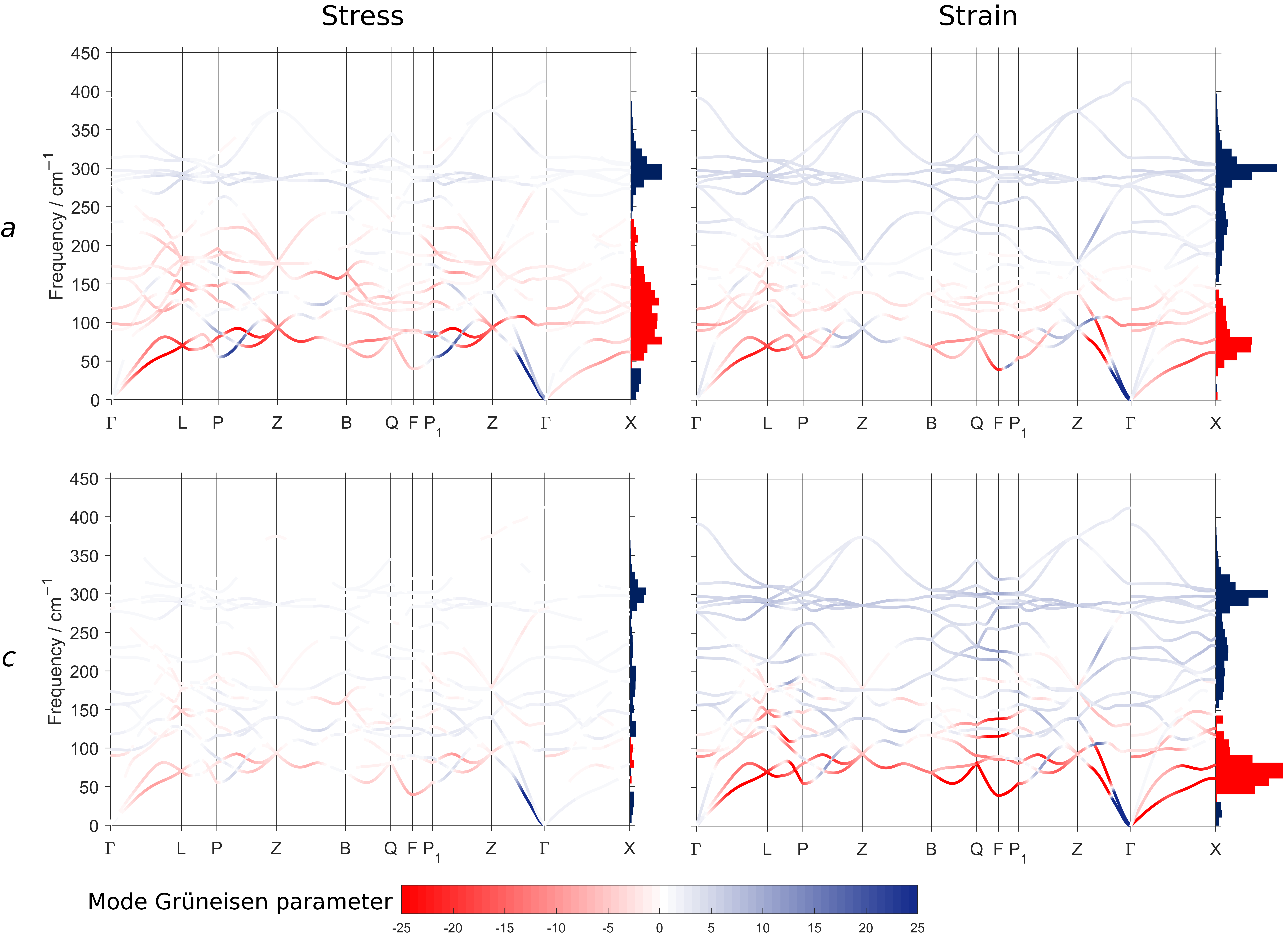
Figure 5: Phonon band structure of calcite, with bands coloured according to their axial mode Grüneisen parameters calculated using stress and strain perturbations. Phonons with energies greater than 450 cm^-1 do not contribute significantly to thermal expansion and are not shown here. The density of states ($\rho$), weighted by the Grüneisen parameters as $\sum_{\mathbf{k}}\rho_{\mathbf{k}}(\omega)\gamma_{n,\mathbf{k}}(\omega)$, is shown as a histogram at the right of each plot, with positive values coloured in blue and negative values in red. Special points in and paths through the Brillouin zone were selected following Ref. 62.

The Grüneisen parameters obtained from the stress perturbations indicate that negative thermal expansion along $a$ is driven by low-energy acoustic and librational modes. Along $c$, the Grüneisen parameters are small and mostly positive; the reduced stiffness along $c$ increases $\alpha_{cc}$. By contrast, the mode Grüneisen parameters related to the strain perturbation along $a$ and along $c$ are similar. Due to the significant Poisson ratios relating $a$ and $c$ ($\nu_{aacc}=0.45$ and $\nu_{ccaa}=0.26$) the stresses transverse to the strain perturbation are of the same order of magnitude as the stresses along the perturbation direction. Therefore, the inaccuracy of the uniaxial strain model in this case indicates that the convolution of the axial Grüneisen parameters through the cross-compliances (Eq. (5)) is inexact.

V Discussion

The similarities and differences between the uniaxial stress perturbation (Eq. (18)) and the uniaxial strain perturbation (Eq. (5)) can be appreciated by considering their application to a simplified model. Fig. 6 shows a square lattice with a positive Poisson ratio and positive thermal expansion, where each bond vibrates independently. When the lattice is subjected to a uniaxial strain perturbation, the bonds aligned with the perturbation elongate and their vibrational frequencies decrease, indicating a positive contribution to $\alpha$. However, a negative contribution to $\alpha$ comes from the bonds orthogonal to the perturbation, proportional to the Poisson ratio relating the two axes. In the uniaxial stress case, the Poisson effect contracts the bonds perpendicular to the perturbation, again resulting in a decrease in $\alpha$ proportional to the Poisson ratio. It can therefore be appreciated that, for this simplified model, Eq. (5) and Eq. (18) are equivalent.

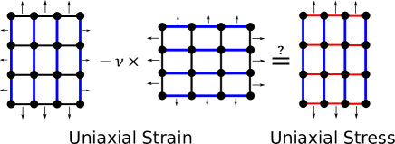
Figure 6: A comparison of the uniaxial strain and stress models for a simplified system with positive thermal expansion and positive Poisson ratio. Bonds coloured in blue are lengthened by the perturbation, leading to a decrease in vibrational frequency and a positive contribution to the bulk Grüneisen parameter, while those coloured in red are contracted by the Poisson effect, increasing their frequency and therefore reducing the Grüneisen parameter.

In the simplified model, the vibrational frequencies are linearly related to the lattice constants. This requires two predicates: that the vibrational frequencies are proportional to interatomic distances, and that the interatomic distances are proportional to the lattice constants. The first is a form of the QHA, stating that phonon energies can be expressed as a function of internal strain coordinates. (Hofmeister and Mao, 2002) The second is geometric: in the simplified model, there are no atomic coordinates which are not fixed by the lattice. If this is not the case, the bond lengths will not, in general, scale linearly with the lattice vectors, and the stress and strain models will be inequivalent. This can occur if the relative positions of the atoms are not fixed by symmetry.

Therefore, the differences between the stress model and the strain model for the materials studied herein (Fig. 2 and Fig. 4) can be explained by their structures. The atomic coordinates of zinc and graphite are fixed by the lattice constants, and therefore are analogous to the simple structure of Fig. 6, and the stress and strain models give results of comparable accuracy. Unlike zinc and graphite, calcite features an internal coordinate not fixed by the lattice constants, and flexible Ca–O–C linkages. This, in combination with the large Poisson ratios in calcite (Fig. 3), leads to the large discrepancy between the two models seen in Fig. 4.

The increased accuracy of the stress model relative to the strain model seen in the ab initio calculations of $\bm{\alpha}$ presented herein can therefore be attributed to the assumption of the strain model that thermal strains along different axes are coupled purely elastically. This treatment ignores that the internal strain coordinates relevant to a particular mode may not have the same elastic behaviour as the lattice. When performing a uniaxial stress perturbation, the Poisson effect is included directly in the model, and no correction for the transverse stresses is required. Since the magnitude of this correction is determined by the cross-compliances, for many systems the difference between the two models is relatively small. However, it will be especially important for materials with unusual elastic properties.

The uniaxial stress model also offers other advantages to the understanding of the origins of thermal expansion. Coupling between thermal expansion and elasticity can be understood in a simpler way, as the Grüneisen parameter along one axis and one element of the compliance tensor determine the CTE in that direction without reference to the transverse axes. Therefore, negative thermal expansion is impossible without modes with negative Grüneisen parameters. In fact, although the strain model allows for negative thermal expansion from positive Grüneisen parameters due to the Poisson effect, the only materials where it has been suggested that this occurs are zinc and cadmium. (Barrera et al., 2005)

The appearance of $s_{ijij}$ in Eq. (18) indicates that directional thermal expansion can be predicted by reference to the directional Young’s moduli ($Y_{ii}={s_{iiii}}^{-1}$). This was perhaps anticipated by Barker Jr., (Barker Jr., 1963) who found that for a broad range of materials the approximate relationship $Y\alpha^{2}\approx 15~{}\text{Pa}$ holds, and that differences in thermal expansivity between materials are often driven by their relative Young’s moduli rather than by differences in the Grüneisen parameter. This approach can be extended by considering, for example, directional Young’s moduli in calcite (Fig. 3) in relation to directional thermal expansion. Fig. 3 and Fig. 1 show that the calcite structure is most stiff along directions corresponding to Ca–O–C linkages. Rotation of $\bm{\alpha}$ shows that the directions of maximum stiffness have very low thermal expansion ($\alpha_{\ell}=6\times 10^{-8}~{}\text{K}^{-1}$). In fact, if by inspection of Fig. 3 one was to assume that the stiffest directions have smaller magnitudes of $\alpha_{\ell}$ than do the principal axes, this would lead to the conclusion that $\alpha_{\ell}$ must be negative along one principal axis and positive along the other, based on the required symmetry of $\bm{\alpha}$ (i.e., that the maxima and minima lie along principal axes).(Nye, 1985)

This analysis can be extended to other orthotropic systems where stiffness maxima are not aligned with the unit cell vectors, e.g. the metal-organic wine-rack framework material MIL-53 has $\alpha_{\ell}=7\times 10^{-7}~{}\text{K}^{-1}$ along the stiff wine-rack axes, leading to anomalous thermal expansion along the compliant principal axes ($\alpha_{bb}=-1.4\times 10^{-5}~{}\text{K}^{-1}$, $\alpha_{cc}=2.4\times 10^{-5}~{}\text{K}^{-1}$).(Nanthamathee et al., 2014) When the Grüneisen parameter along the stiffest direction is anomalous, even more unusual behaviour can occur. For example, Ag₃Co(CN)₆ has $\alpha_{\ell}=-2.5\times 10^{-5}~{}\text{K}^{-1}$ along a Co–CN linkage (a typical value for an M–CN chain);(Chippindale et al., 2012) this, along with the compliance of the $ab$ plane, results in colossal positive and negative thermal expansion along the principal axes ($\alpha_{aa}=1.4\times 10^{-4}~{}\text{K}^{-1}$, $\alpha_{cc}=-1.3\times 10^{-4}~{}\text{K}^{-1}$).(Goodwin et al., 2008) This misalignment mechanism can be expected to occur commonly in materials which exhibit negative linear compressibility, which requires a mixture of stiff and compliant directions to balance stability and flexibility.(Cairns and Goodwin, 2015) Of course, the phenomenon is essentially geometric, and coincides with the geometric arguments previously used to explain anomalous thermal expansion in these materials.(Goodwin et al., 2008; Nanthamathee et al., 2014) However, removing the cross-coupling term of the strain model facilitates understanding of relationships between thermal expansion anisotropy and framework flexibility by removing the need to consider the (often large) Poisson ratios directly.

The stress model has an additional advantage over the strain model in that one element of $\bm{\alpha}$ can be calculated independently of the others. This offers the possibility of, for example, calculating one element in order to understand the mechanisms of uniaxial negative thermal expansion,(Senn et al., 2015) or to test the accuracy of an exchange-correlation functional or a set of pseudopotentials for a given system. Especially for monoclinic and triclinic crystal families, the computational expense required to calculate Grüneisen parameters for every element of $\bm{\alpha}$ may be prohibitive, but a qualitative understanding of thermoelastic behaviour could perhaps be obtained with some subset thereof.

VI Conclusions

A Grüneisen model for anisotropic materials based on uniaxial strain perturbations has been proposed. This model has the advantage of including the mechanical coupling between axes explicitly, allowing the thermal expansion axis to be related to mode Grüneisen parameters and the Young’s modulus in that direction only. The model was tested by ab initio prediction of thermal expansion in several highly anisotropic materials; revealing that the uniaxial stress model has equal or better accuracy to the previous uniaxial strain model. By relating the directional Young’s moduli to thermal expansion directly, it can be predicted that framework materials whose rigid units are misaligned with the principal axes are likely to display positive and negative axial thermal expansion.