ELDAR, a new method to identify AGN in multi-filter surveys: the ALHAMBRA test-case

Abstract

We present ELDAR, a new method that exploits the potential of medium- and narrow-band filter surveys to securely identify active galactic nuclei (AGN) and determine their redshifts. Our methodology improves on traditional approaches by looking for AGN emission lines expected to be identified against the continuum, thanks to the width of the filters. To assess its performance, we apply ELDAR to the data of the ALHAMBRA survey, which covered an effective area of $2.38\,{\rm deg}^{2}$ with 20 contiguous medium-band optical filters down to F814W $\simeq 24.5$. Using two different configurations of ELDAR in which we require the detection of at least 2 and 3 emission lines, respectively, we extract two catalogues of type-I AGN. The first is composed of 585 sources ($79\,\%$ of them spectroscopically-unknown) down to F814W $=22.5$ at $z_{\rm phot}>1$, which corresponds to a surface density of $209\,{\rm deg}^{-2}$. In the second, the 494 selected sources ($83\,\%$ of them spectroscopically-unknown) reach F814W $=23$ at $z_{\rm phot}>1.5$, for a corresponding number density of $176\,{\rm deg}^{-2}$. Then, using samples of spectroscopically-known AGN in the ALHAMBRA fields, for the two catalogues we estimate a completeness of $73\,\%$ and $67\,\%$, and a redshift precision of $1.01\,\%$ and $0.86\,\%$ (with outliers fractions of $8.1\,\%$ and $5.8\,\%$). At $z>2$, where our selection performs best, we reach $85\,\%$ and $77\,\%$ completeness and we find no contamination from galaxies.

1 Introduction

Active galactic nuclei (AGN) are among the brightest objects in the Universe. They are powered by the accretion of matter onto a supermassive black hole (SMBH): as the gas approaches the SMBH, its temperature rises and starts to emit radiation across the entire electromagnetic spectrum. Nevertheless, AGN not only show a continuum emission from the gas in the accretion disk, but they also exhibit multiple emission lines from the X-ray to the infrared spectral range. In turn, the emission lines may be broad or narrow, depending on the orientation of the AGN with respect to the observer and the obscuring material (according to the AGN unification scheme, Antonucci, 1993; Urry & Padovani, 1995). AGN with broad emission lines are referred to as “type-I”, while AGN with just narrow emission lines as “type-II”. We will employ this observational classification along the rest of the paper.

For their many applications in different fields of astrophysics, from high-energy physics to cosmology, a complete census of AGN is fundamental. AGN are studied in the context of galaxy evolution models (e.g., Heckman & Best, 2014), as there are evidences of tight correlations between SMBH and galaxy properties (e.g., Kormendy & Richstone, 1995; Gebhardt et al., 2000), although a causal origin of these correlations is not universally accepted (e.g., Peng, 2007; Jahnke & Macciò, 2011). In addition, thanks to their large luminosities, the optically brightest type-I AGN (commonly referred to as quasars) allow us to trace the matter distribution since early times (currently, the most distant spectroscopically-confirmed quasar is at $z=7.1$, see Mortlock et al., 2011). Quasars can also be used to constrain cosmology: Busca et al. (2013) successfully detected Baryonic Acoustic Oscillations (BAO) in the Ly $\alpha$ forest, and future galaxy surveys plan to measure the BAO feature through the clustering of quasars (e.g., the Extended Baryon Oscillation Spectroscopic Survey is expected to reach a $1.6\,\%$ precision measuring spherically averaged BAO with quasars, see Dawson et al., 2016; Zhao et al., 2016). Finally, they have even been proposed as standard candles (Wang et al., 2014; Watson et al., 2011; Risaliti & Lusso, 2017).

There are many techniques for detecting AGN, such as traditional colour-colour selections (e.g., Matthews & Sandage, 1963), optical variability (e.g., Schmidt et al., 2010), and the combination of optical data and observations in radio (e.g., White et al., 2000), X-ray (e.g., Barger et al., 2003; Brusa et al., 2003), and/or infrared (e.g., Lacy et al., 2004). The strengths and weaknesses of these methods are different. For instance, X-ray selection allows to be complete, missing only the most obscured sources, at the cost of being very time consuming. On the other hand, broad-band photometric surveys are less time-expensive but they are biased towards unobscured type-I AGN, and they include a significant contamination from stars and galaxies.

The emergence of multi-filter surveys, such as the Classifying Objects by Medium-Band Observations - a spectrophotometric 17-filter survey - (COMBO-17, Wolf et al., 2004, 2008), the Cosmic Evolution Survey (COSMOS, Scoville et al., 2007), the Advance Large Homogeneous Area Medium Band Redshift Astronomical survey (ALHAMBRA, Moles et al., 2008), the Survey for High-$z$ Absorption Red and Dead Sources (SHARDS, Pérez-González & Cava, 2013), the Physics of the Accelerating Universe Survey (PAUS, Martí et al., 2014), and the upcoming Javalambre Physics of the Accelerating Universe Astrophysical Survey (J-PAS, Benítez et al., 2014), open the possibility of exploring new methods for detecting AGN. Multi-band photometric data, in fact, combine the strengths of broad-band photometric and spectroscopic surveys, resulting in a low-resolution spectra for every pixel of the sky observed, e.g. the ALHAMBRA survey has spectral resolution of $R=310$. The aim of this work is precisely to produce a new pipeline to identify AGN and to compute their redshifts using just data from multi-filter surveys. We take advantage of the low-resolution spectroscopic nature of these data in order to identify strong spectral features typical of active galaxies.

We test our new algorithm, dubbed as Emission Line Detector of Astrophysical Radiators (ELDAR), by applying it to the data from the ALHAMBRA survey (Moles et al., 2008; Molino et al., 2014). This survey is an optimal test-case for ELDAR because it observed $\simeq 4\,{\rm deg}^{2}$ using 20 contiguous medium-band filters (Full Width Half Maximum FWHM $\simeq 300\,\rm{\AA}$) in the optical range and 3 broad-band filters ($J$, $H$, and $K_{s}$) in the infrared. In addition, Matute et al. (2012) showed that it is possible to compute precise redshifts ($\sigma_{\rm NMAD}\simeq 1\,\%$) for spectroscopically-known quasars using just ALHAMBRA data. Here, we extract two catalogues of type-I AGN using two different ELDAR configurations, the first maximising completeness and the second minimising contamination. Then, we analyse the main properties of these catalogues and we estimate their completeness, redshift precision, and galaxy contamination by applying the same ELDAR configurations to samples of spectroscopically-known type-I AGN and galaxies within the ALHAMBRA fields.

This paper is structured as follows. In §2 we introduce ELDAR and in §3 we tune our method to detect type-I AGN in ALHAMBRA. In §4 we extract two catalogues of type-I AGN and we characterise their properties. In §5 we discuss the potential of our methodology for surveys with narrower bands and in §6 we summarise our conclusions.

Throughout this paper the optical and near-IR magnitudes are in the AB system, we always use the spectral flux density per unit wavelength, and we assume a six parameter $\Lambda$CDM cosmology with $H_{0}=67.8\,\text{km s}^{-1}\text{Mpc}^{-1}$, $\Omega_{\Lambda}=0.692$, and $\Omega_{\rm M}=0.308$ (Planck Collaboration et al., 2016).

2 ELDAR algorithm

The new methodology to detect AGN in multi-filter surveys that we introduce in this paper, ELDAR, consists of two main steps: i) template-fitting, that aims at pre-selecting AGN candidates and at obtaining a redshift probability distribution function (PDZ) for each of them, and ii) spectro-photometric confirmation, whose objective is to securely confirm the previous candidates by detecting typical AGN emission lines in the multi-band photometric data and to refine the photo-$z$ estimation.

In what follows, we describe in more detail the two steps of ELDAR.

2.1 Template-fitting step

The main purpouse of this first step is to pre-select AGN candidates and to obtain a PDZ for each of them. While any template-fitting code may be used for this pre-selection phase, in this work we adopt the code PHotometric Analysis for Redshift Estimate (LePHARE) (Arnouts et al., 1999). LePHARE is a template-fitting code extensively used to compute photo-$z$s for galaxies and AGN (e.g., Ilbert et al., 2009; Salvato et al., 2009, 2011; Fotopoulou et al., 2012; Matute et al., 2012). Here we provide a general discussion on how to correctly configure LePHARE, as the templates and parameters of the code have to be carefully chosen and optimised to detect AGN depending on the characteristics of the survey to be analysed. In addition, in §3.3 we provide the specific configuration of LePHARE for the case of the ALHAMBRA survey.

• Template selection. LePHARE classifies each source and computes its redshift depending on the Spectral Energy Distribution (SED) of the template that produces the best-fit to the photometric data, where a template is a theoretical or empirical curve that describes the flux of different astronomical objects as a function of $\lambda$. The library of templates to be used in LePHARE has to be meticulously chosen, especially when working with AGN (Hsu et al., 2014): while it should be comprehensive enough to include the broad variety of SEDs of the types of sources that are sought, the number of templates should not be too large to avoid degeneracies.

  The templates are divided into two main categories in LePHARE: stellar and extragalactic. The first includes the SEDs of stars, while the second presents the SEDs of extragalactic objects at rest-frame, which are shifted in redshift during the fitting procedure. To build our stellar library we include 254 stellar templates from the publicly available distribution of LePHARE. They are divided into 131 templates of normal stellar spectral types and luminosity classes at solar abundance, metal-poor F-K dwarfs, and G-K giants (Pickles, 1998); 4 templates of white dwarfs (Bohlin et al., 1995); 100 templates of low mass stars (Chabrier et al., 2000); and 19 templates of sub-dwarfs (Bixler et al., 1991). We include all of them to cover as many stellar types as possible and thus, to avoid the classification of stars as AGN.

  For the extragalactic library, we only include templates of active galaxies, as these are the sources we are targeting. With this approach, we ensure that no AGN are wrongly classified as ‘normal’ galaxies (i.e. galaxies whose SEDs are not dominated by nuclear activity), while all normal galaxies will be discarded by the spectro-photometric confirmation step (see §2.2). The AGN templates to be included in the extragalactic library are survey specific, as the AGN types that can be unambiguously confirmed in a given survey depend on its characteristics, e.g., its depth, area, and the width of its photometric bands. In particular, the width of the survey bands determines the approximate minimum Equivalent Width (EW) of the emission lines that can be detected by ELDAR (see §3.3). As the EWs of AGN emission lines depend on the type of active galaxy, we should only include templates of AGN with emission lines strong enough to be detected by our method.

• Redshift range and precision. The extragalactic templates included in the LePHARE library are located at rest-frame. During the fitting procedure, LePHARE creates a grid of templates displaced in redshift, where the redshift step and maximum redshift are defined by the user. As Benítez et al. (2009) observed, the size of the redshift step should depend on the number of filters available and the overlap between them. As for the maximum redshift, we set it to the redshift above which no strong spectral features appear to within the survey wavelength coverage.

  Effectively, the PDZ generated by LePHARE is defined as:

  $${\rm\small PDZ}(z)=\frac{G(z)}{G(z_{\rm best})},$$ (1)

  where $G(z)=\exp[-\chi^{2}_{\rm min}(z)/2]$, $\chi^{2}_{\rm min}(z)$ is the $\chi^{2}$ resulting from the template that best fits the data at redshift $z$, and $z_{\rm best}$ is the redshift at which the data is best-fitted. With this definition, the PDZ is not properly a probability density function, and to generate one for each object the PDZ of the previous expression should be normalised by its integral.

• Dust attenuation. The extinction law of AGN varies as a function of redshift (e.g., Gallerani et al., 2010), reflecting different mechanisms for dust production and/or destruction. A correct modelling of the effect of dust is required because it absorbs UV and optical light, which then re-emits in the infrared modifying the SEDs of AGN. In LePHARE we employ the Milky Way (Allen, 1976), Small Magellanic Cloud (Prevot et al., 1984), Large Magellanic Cloud (Fitzpatrick, 1986), and starburst (Calzetti et al., 2000) extinction laws, which are shown in fig. 7 of Bolzonella et al. (2000).

  The dust attenuation ($A_{V}$) of an active galaxy depends on its orientation with respect to the observer and it is defined as

  $$A_{V}=R_{V}\times E(B-V),$$ (2)

  where $E(B-V)$ is the colour excess and $R_{V}$ is a coefficient that depends on the extinction law. We introduce colour excesses from $0$ to $0.10$ in steps of $0.02$, from $0.10$ to $0.30$ in steps of $0.04$, and from $0.30$ to $1.00$ in steps of $0.10$. We include colour excesses as high as 1 to account for very extinct AGN. We set finer steps for low colour excesses because some AGN templates are empirical, and thus they already include some extinction.

• Luminosity prior. Setting luminosity priors is important to avoid unrealistic solutions (Salvato et al., 2009), and they should be chosen depending on the type of objects that we want to target. Quasars, for example, are traditionally defined as objects with $M_{B}\leq-23$ (e.g., Osterbrock, 1991), and setting $M_{B}=-23$ as upper limit ensures that LePHARE rejects low redshift (low-$z$) incorrect solutions.

2.2 Spectro-photometric confirmation step

Objects with strong emission lines, such as type-I AGN, are particularly suited to be detected in surveys with contiguous medium- and/or narrow-band filters. This is because emission lines with a large EW completely dominate the bands in which they fall. Consequently, these bands appear as clear ‘peaks’ in the multi-band data. The height of these peaks with respect to the continuum emission depends on i) the EW of the line, ii) the width of the band where the emission line falls, and iii) the shape of the continuum. Assuming that the AGN continuum emission is flat in the bands adjacent to the band where the line falls, ELDAR is able to detect lines with EW greater than

$${\rm EW}_{\rm min}=\frac{B_{\rm FWHM}}{(1+z)B_{\rm SNR}}\sigma_{\rm line},$$ (3)

where $B_{\rm FWHM}$ is the FWHM of the band where the line falls, $B_{\rm SNR}$ is the Signal-to-Noise Ratio (SNR) in this band, $z$ is the redshift of the source, and $\sigma_{\rm line}$ is a parameter that denotes the confidence with which we want to confirm lines, e.g. $\sigma_{\rm line}=1$ means a $1\,\sigma$ detection. Therefore, the detection of emission lines depends on the intrinsic properties of each source (e.g. their $z$ and EW) and on the characteristics of the survey to be analysed (e.g. the bandwidth of the bands and their depth.

However, Eq. 3 just sets an approximate value for ${\rm EW}_{\rm min}$. This is because the assumption of a flat continuum is not usually correct for AGN, especially at $z<2.5$ where the slope of the AGN continuum is very steep and blue. Moreover, the value of ${\rm EW}_{\rm min}$ is also an lower limit for emission lines that fall in between two bands or are broader than the survey bands.

With these caveats in mind, the objective of this second step of ELDAR is to search for typical AGN emission lines in the multi-band photometry of the sources that we want to classify. We improve on the ability of template fitting codes in unambiguously confirm emission line objects, as they do not include special weights for the bands where emission lines fall and, as the number of bands dominated by the continuum emission is always greater than the number of bands dominated by emission lines, they are not specifically designed for detecting these objects.

The detection of AGN emission lines allows not only to confirm sources as active galaxies but also to reject stars and galaxies assigned to AGN templates in the first step of ELDAR. Moreover, it provides a method to discriminate between different redshift solutions given by the PDZ. Operationally, the confirmation step works as follows:

1. We start by selecting, for each source, the redshifts at which the SED is best-fitted by an extragalactic template ($\chi^{2}_{\rm AGN}<\chi^{2}_{\rm star}$) and the value of the PDZ is greater than 0.5. We set a lower limit in the PDZ in order to include the information provided by LePHARE from the fitting of the SED. We check the dependence of the results on different PDZ lower limits in Appendix B. For each of these possible redshift solutions, $z_{\rm guess}$, we perform the steps that follow.

2. According to each $z_{\rm guess}$, we calculate which AGN emission lines with EW greater than ${\rm EW}_{\rm min}$ are expected to lie within the wavelength coverage of the survey, and in which band they should fall. We then confirm the detection of a line if:

   $$F_{\rm cen}>\left\{\begin{aligned} &F_{\rm blue}+\sigma_{\rm line}\,S_{\rm cen},\\ &F_{\rm red}+\sigma_{\rm line}\,S_{\rm cen},\\ &F_{\rm blue}+\sigma_{\rm line}\,S_{\rm blue},\\ &F_{\rm red}+\sigma_{\rm line}\,S_{\rm red},\\ \end{aligned}\right.$$ (4)

   where $F_{\rm cen}$ is the flux in the band where the line should fall according to $z_{\rm guess}$, $F_{\rm blue}$ ($F_{\rm red}$) is the flux in the band bluewards (redwards) of the band where the line should fall, and $S_{\rm cen}$, $S_{\rm blue}$, and $S_{\rm red}$ are their errors. By construction, we are unable to confirm lines that fall either in the first or in the last band of the filter system.

   

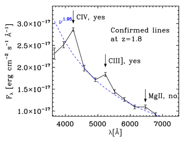
   Figure 1: Multi-band ALHAMBRA photometry of a spectroscopically-known type-I AGN at $z=1.8$. At this redshift, the lines C IV, C III], and Mg II fall within the ALHAMBRA medium-band wavelength range. ELDAR confirms C IV and C III] with more than $1\,\sigma$ confidence in the 3rd and 6th band, respectively. On the other hand, Mg II is not confirmed because the flux in the 9th band, where this line should fall according to $z_{\rm spec}$, does not fulfil all the requirements of Eq. 4. The blue dashed line shows a power law to guide the eye on the AGN continuum.

   

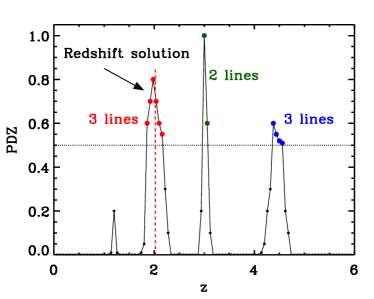
   Figure 2: Illustrative example of a PDZ in which we include information about the number of AGN emission lines detected by ELDAR. The black small dots indicate redshift solutions with PDZ $<0.5$, the green dots solutions with PDZ $>0.5$ for which ELDAR detects 2 AGN emission lines, and the red and blue dots solutions with PDZ $>0.5$ for which ELDAR detects 3 AGN emission lines. The red dashed line shows the final redshift solution for the source, $z_{\rm phot}$. See the text for further information about how $z_{\rm phot}$ is computed.

   In Fig. 1 we show a spectroscopically-known type-I AGN at $z_{\rm spec}=1.8$ observed by the ALHAMBRA survey (we will present the characteristics of the survey in §3.1). We show arrows pointing to the bands where C IV, C III], and Mg II should fall according to $z_{\rm spec}$. The blue dashed line indicates a power law that guides the eye on the AGN continuum emission and it allows us to easily see the flux excess in the bands where the AGN emission lines fall. For this source, C IV and C III] are detected by ELDAR while Mg II is not confirmed because it does not fulfil all the requirements of Eq. 4.

   There are some redshift intervals for which two different emission lines may fall in consecutive bands, and thus the line detection is not secure. However, the typical separation between the strongest AGN emission lines (EW $>8$) with rest-frame central wavelength $\lambda_{\rm c}<4\,000\,{\rm\AA}$ is large enough for these lines to never fall in consecutive bands in surveys with filters narrower than FWHM $\sim 400\,{\rm\AA}$. In any case, if lines with different EW fall in consecutive bands, the line with the largest EW can still be confirmed.

   In surveys with no contiguous bands another complication might arise at redshifts in which AGN emission lines fall between two bands, as the flux of the line gets dispersed. However, in most cases the greatest part of the line falls in one band and just its tail in other/s. In this case, the line is detected in the band where the greatest part of its flux falls. We further explore this issue in §5.

   To account for redshift errors and physical processes that may displace emission lines from the band where they should fall, such as line shifts and anisotropic profiles (see Vanden Berk et al., 2001), we search for emission lines not only in the band where they should fall according to $z_{\rm guess}$, but also in the two adjacent bands.

3. We confirm as AGN the sources for which we detect at least $\mathcal{N}$ emission lines at the expected redshift, where $\mathcal{N}$ is chosen depending on the number of lines that the survey filter system allows to detect, as well as on a compromise between the completeness and the level of galaxy and star contamination that we want to achieve. Obviously, the contamination from galaxies and stars decreases by increasing $\mathcal{N}$ (see §3.2 for a discussion about potential contaminants for the ALHAMBRA survey).

4. Once a source is confirmed as AGN, we check at which $z_{\rm guess}$ the largest number of lines is detected, rejecting the other values. If we end up with a single $z_{\rm guess}$, we accept it as the final photo-$z$ solution, $z_{\rm phot}$. Otherwise, we group contiguous $z_{\rm guess}$ into intervals, and we look for the interval with the greatest average PDZ. In this case, we then compute the final redshift solution as

   $$z_{\rm phot}=\frac{\sum_{i}^{n}\,z_{{\rm guess},i}\,{\rm\small PDZ}(z_{{\rm guess},i})}{\sum_{i}^{n}\,{\rm\small PDZ}(z_{{\rm guess},i})},$$ (5)

   where the summation goes through the $n$ values of $z_{\rm guess}$ in the selected interval.

In Fig. 2 we show an illustrative example of this procedure. We start by selecting $z_{\rm guess}$, i.e. the redshifts at which the SED of the object is best-fitted by an AGN template and the value of the PDZ is greater than 0.5. These redshift solutions are the red, green, and blue points. Then, we pick the $z_{\rm guess}$ for which the largest number of lines is detected (in this example, the red and blue dots). After that, we group the red points into one interval and the blue ones into another. Later, we reject the blue-points interval because the mean PDZ of the red-points interval is greater. Finally, we compute $z_{\rm phot}$ with the red-points interval using Eq. 5.

The above steps define the backbone of the spectro-photometric confirmation. Additional criteria can be added to refine the procedure. For instance, as the Ly $\alpha$ line is the strongest AGN emission line in the UV, in the present work we require i) the Ly $\alpha$ line to be detected in sources with redshift solutions for which this line should fall within the survey wavelength coverage, and ii) the flux in the band where it falls to be at least $75\,\%$ of the maximum flux in any of the other bands. Even if the Ly $\alpha$ line is the strongest in the UV, we set a $75\,\%$ limit to account for the possibility of the line falling in between two bands and/or other emission lines surpassing its flux. With this condition we want to reject cold stars whose continuum emission may be confused with the Lyman-break of high-$z$ AGN. We explore the dependence of the results on this criterion in Appendix B.

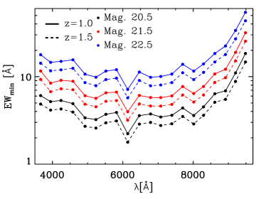
Figure 3: Minimum EW of the emission lines that can be detected in each ALHAMBRA optical band for $\sigma_{\rm line}=1$, as a function of the magnitude of the band and the redshift of the source.

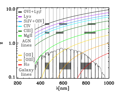
Figure 4: Evolution of the central wavelength of AGN and galaxy emission lines as a function of redshift. We also display the transmission curves of the ALHAMBRA medium-band filters, which allow us to see in which band the emission lines are located as a function of $z$. The grey areas highlight the redshift intervals for which there is a degeneracy among the triplet of galaxy emission lines {[O II], [O III], H $\alpha$}, and the triplets of AGN emission lines {C IV, C III], Mg II} and {O VI+Ly $\beta$, Si IV]+O IV], C III]}.

3 Applying ELDAR to ALHAMBRA data

In the previous section we introduced ELDAR, our new procedure to detect AGN. Here, we introduce the ALHAMBRA survey, we discuss some effects that may affect the quality of ELDAR’s results, and we show how we have optimised our method for analysing the ALHAMBRA data. In §4 we will blindly apply the configurations introduced in this section to the ALHAMBRA data in order to extract a new catalogue of type-I AGN.

3.1 The ALHAMBRA survey

ALHAMBRA is a medium-band photometric survey that observed $\simeq 4\,\text{deg}^{2}$ of the sky distributed over 8 non-overlapping fields. These fields were selected to be in common with other surveys, such as the Deep Extragalactic Evolutionary Probe 2 (DEEP2), the Sloan Digital Sky Survey (SDSS), COSMOS, the Hubble Deep Field North (HDF-N), the Deep Groth Strip Survey (GROTH), and the European Large Area ISO Survey (ELAIS). The ALHAMBRA filter system consists of 20 contiguous medium-band filters of width $\simeq 300\,\rm{\AA}$, which cover the optical range from $3\,500$ to $9\,700\,\rm{\AA}$, and the 3 broad-band infrared filters $J$, $H$, and $K_{s}$. The magnitude limit ($5\,\sigma$, 3”) is $\simeq 23.7$ for the blue optical filters, $\simeq 22.2$ for the red optical filters, and $\simeq 22$ for the infrared filters (Aparicio Villegas et al., 2010). Due to the width of its filters and the contiguous wavelength coverage from the near UV to the near-infrared, the ALHAMBRA survey is an optimal test-case for ELDAR.

The last public data release of ALHAMBRA is introduced in Molino et al. (2014, M14 hereafter). It covered an area of $\simeq 3\,\text{deg}^{2}$ over 7 fields, detecting $438\,356$ sources brighter than 24.5 mag in the synthetic detection band, F814W. This band was generated by combining the 9 reddest ALHAMBRA bands to mimic the Hubble Space Telescope (HST) - Advanced Camera for Surveys (ACS) F814W band.

The ALHAMBRA filter system produces precise redshift estimates for blue and red galaxies, as shown by M14. Specifically, M14 found a redshift precision of $\sigma_{z}\simeq 1\,\%$ for spectroscopically-known galaxies with F814W $<22.5$ within the ALHAMBRA fields. Moreover, in a first attempt to characterise the ability of ALHAMBRA to produce precise photo-$z$s for type-I AGN, Matute et al. (2012) applied LePHARE to a sample of 170 spectroscopically-known type-I AGN within the ALHAMBRA fields, finding a redshift precision of the same order as for galaxies.

As we stated in the previous section, the properties of the survey filter system are essential to determine i) the approximate minimum EW of the emission lines that can be detected and ii) the redshift precision that can be achieved. In Fig. 3 we show an estimation of the minimum equivalent width of an emission line that can be detected in each ALHAMBRA medium-band (as defined in Eq. 3), as a function of the redshift of the source, its magnitude, and using $\sigma_{\rm line}=1$. By definition, the value of ${\rm EW}_{\rm min}$ decreases for bright sources (higher SNR) and at high-$z$. In addition, the value of ${\rm EW}_{\rm min}$ grows for the reddest bands. This is because the efficiency of the ALHAMBRA CCDs significantly decreases for $\lambda>9\,000\rm{\AA}$ (see the overall transmission of the ALHAMBRA filter system in Fig. 4).

Table 1: Emission lines employed to confirm type-I AGN in ALHAMBRA. At least 2 and 3 emission lines must be detected to validate objects using the ELDAR’s 2- and 3-lines mode, respectively (see §3.3).

Line	$\lambda_{\rm c}(\rm{\AA})$	$\left<{\rm EW}(\rm{\AA})\right>$
O VI+Ly $\beta$	1030	15.6$\pm$0.3
Ly $\alpha$	1216	91.8$\pm$0.7
Si IV+O IV]	1397	8.13$\pm$0.09
C IV	1549	23.8$\pm$0.1
C III]	1909	21.2$\pm$0.1
Mg II	2799	32.3$\pm$0.1

Notes. The values of the central wavelengths and EWs are computed using 184 quasars observed by the HST (emission lines with $\lambda_{\rm c}<1300\,{\rm\AA}$, Telfer et al., 2002) and $2\,000$ quasars observed by SDSS (emission lines with $\lambda_{\rm c}>1300\,{\rm\AA}$, Vanden Berk et al., 2001).

In Table 1 we list the AGN emission lines that are potentiality detectable with at least $1\,\sigma$ precision for i) sources with magnitude $\lesssim 21.5$ in the band where the line falls, and ii) an observed central wavelength, $\lambda_{\rm obs}=\lambda_{c}(1+z)$, smaller than $9\,000\,{\rm\AA}$. In addition, as the ALHAMBRA bands are contiguous, these lines can be detected for the entire redshift interval where they fall within the ALHAMBRA optical coverage. We do not look for emission lines with $\lambda_{\rm c}>3\,000\,{\rm\AA}$, such as [O II], H$\beta$, [O III], or H $\alpha$, because these lines also appear in star-forming galaxies. Whereas it is possible to use them to discriminate between type-I AGN and star-forming galaxies as the lines of type-I AGN are much broader, the low spectral resolution of ALHAMBRA prevent us to employ them (we expect this to be possible in surveys with narrower bands). Therefore, given the lines that we can use to detect AGN and their strengths, we will be able to securely identify type-I AGN at $z>1$ (unobscured broad emission line AGN with no or very little contribution from the host). As a consequence, we focus on the detection of type-I AGN in this work, and we tune ELDAR accordingly.

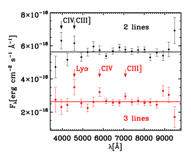
Figure 5: Two ALHAMBRA mock realisations of a source with a flat SED and F814W $=21.5$. The black points show fluxes measured in each ALHAMBRA medium-band in the first realisation and the red squares in the second. The measured fluxes are not on the top of the solid lines, which indicate the underlying SED of the mock source, due to photometric errors. The arrows point to bands where ELDAR detects emission lines with $1\,\sigma$ significance, and the names indicate with which AGN emission lines these spurious lines could be confused. The fluxes of the first (second) realisation are displaced $+(-)1.5\times 10^{-18}\,{\rm erg\,cm^{-2}s^{-1}\AA^{-1}}$ for visual purposes. We show these two examples because these objects could be confirmed as AGN by ELDAR due to the presence of spurious lines.

3.2 Effects that may reduce the redshift precision and increase the contamination from galaxies

Before optimising ELDAR for detecting type-I AGN in the ALHAMBRA survey, we will explore three effects that may decrease the quality of the ELDAR’s results: i) confusion between pairs/triplets of AGN and galaxy emission lines, which increases contamination from galaxies; ii) confusion between different pairs/triplets of AGN emission lines, which reduces the redshift precision; and iii) detection of spurious lines, which may reduce the redshift precision and introduce galaxy contamination. There are examples of all of these issues in Appendix A.

The confusion between different pairs/triplets of emission lines arises due to the limited spectral resolution of multi-filter surveys. The misidentification appears at redshifts where the relative difference between the central wavelengths of different pairs/triplets of emission lines is the same, and thus they fall in the same survey bands. The number and width of these redshift intervals depend on the width of the survey bands, where the narrower the bands the smaller the incidence. In Fig. 4 we display the observed central wavelength of several AGN and galaxy emission lines as a function of $z$. Moreover, we plot the transmission curves of the ALHAMBRA medium-band filters. They guide the eye to see the band where different emission lines fall as a function of $z$. The grey areas highlight the redshift interval for which a triplet of galaxy emission lines can be confused with triplets of AGN emission lines. This is at $z\simeq 0.2$ where the galaxy emission lines {[O II], [O III], H $\alpha$} can be confused with the AGN lines {C IV, C III], Mg II} at $z\simeq 2$ and {O VI+Ly $\beta$, Si IV+O IV], C III]} at $z\simeq 3.5$.

The incidence of line misidentification for pairs of galaxies and AGN emission lines is much higher than for triplets, causing low-$z$ low-$z$ star-forming galaxies to be confused with high-$z$ type-I AGN. This is important because the number density of star-forming galaxies is much greater than the number density of type-I AGN. In addition, misidentification of AGN emission lines may lead to catastrophic redshift solutions. We study this in detail in §4.2.1.

Finally, the presence of spurious lines in the multi-band data can be a possible source of mis-classification. We define a spurious line as a line detected by ELDAR in a band where no emission lines should fall according to $z_{\rm spec}$. They mostly appear due to photometric errors, and their incidence depends on the criterion chosen to confirm emission lines, $\sigma_{\rm line}$, where the smaller its value the higher the frequency. The also may appear due to the blending of two sources or stellar spikes.

To get a rough estimation of the impact of spurious lines in ALHAMBRA, we consider the case of a mock source with a flat SED. Then, we compute the magnitude and uncertainty in each ALHAMBRA medium-band, where the uncertainties are computed using ALHAMBRA empirical errors. After that, we perturb the magnitude in each band $10^{5}$ times using Gaussian distributions with width equal to the $1\,\sigma$ uncertainty in the band, generating $10^{5}$ random realisations of the mock source. In Fig. 5 we show two of these realisations. In the first one, ELDAR detects spurious lines in the 2nd and 4th bands, the same bands where {C IV, C III]} fall at $z=1.48$. In the second, ELDAR confirms spurious lines in the 4th, 8th, and 12th bands, the same bands where {Ly $\alpha$, C IV, C III]} fall at $z=2.76$. Therefore, these objects could be wrongly classified as type-I AGN by certain configurations of ELDAR. Moreover, the incidence of spurious confirmations is even higher for objects with real emission lines.

The number of sources wrongly confirmed as type-I AGN due to spurious lines depends on $\sigma_{\rm line}$ and $\mathcal{N}$, where the higher their values the lower the contamination. Therefore, it is very important to take this into account before choosing the value of $\mathcal{N}$ and $\sigma_{\rm line}$. In addition, another effect that increases the number of spurious lines is a bad calibration of the zeropoints of the survey bands; however, this is not an issue for us because the values ALHAMBRA zeropoints are very robust (for a detailed discussion see M14).

3.3 Specific configuration of ELDAR for the ALHAMBRA survey

Here we configure ELDAR to identify type-I AGN in the ALHAMBRA survey. In order to do this, we start by optimising LePHARE, and then we tune the configuration of the spectro-photometric step to extract two samples of type-I AGN, where the first prioritises completeness and the second a reduced galaxy contamination.

Given the width of the ALHAMBRA bands, the only type of AGN that we can securely detect are the ones with broad emission lines, i.e. type-I AGN. Consequently, we will only introduce templates describing the SED of these objects in the extragalactic library of LePHARE. Specifically, we select the empirical templates of quasars and AGN used in Salvato et al. (2009, 2011) and the synthetic templates of quasars included in the LePHARE distribution. The resulting library encompasses 49 templates, where 31 of them are synthetic templates that employ different power laws for the AGN continuum and EWs for the emission lines. From this list, we select the templates that give the best results in terms of completeness and redshift precision for a sample of spectroscopically-known AGN within the ALHAMBRA fields, which we call AGN-S.

The AGN-S sample is obtained by performing a crossmatch between the spectroscopically confirmed point-like type-I AGN (sources with Q or A flags) from the Million Quasar Catalogue (MQC, Flesch, 2015, references within) and the ALHAMBRA sources with F814W $<23$. The MQC is a largely complete compendium of AGN from the literature through 21 June 2016. We do the match for objects separated by less than 2 arcsec and, in the two cases where we find two ALHAMBRA sources within 2 arcsec of the MQC object, we visually confirm the match by looking at the ALHAMBRA photometry (in both cases we validate the match with blue objects that clearly exhibit broad emission lines). In addition, we also perform a crossmatch between the ALHAMBRA sources with F814W $<23$ and the 637 type-I AGN from the COSMOS-Legacy X-ray catalog (C-COSMOS) (Civano et al., 2016; Marchesi et al., 2016) with an optical counterpart and spectroscopic redshift, following the same matching procedure as for the MQC. We end up with a total of 295 sources for the AGN-S sample.

Table 2: Extragalactic templates that we introduce in LePHARE.

Index	Template	Class
1	I22491_70_TQSO1_30	Quasar $30\,\%$ + Gal. $70\,\%$[1]
2	I22491_60_TQSO1_40	Quasar $40\,\%$ + Gal. $60\,\%$[1]
3	I22491_50_TQSO1_50	Quasar $50\,\%$ + Gal. $50\,\%$[1]
4	I22491_40_TQSO1_60	Quasar $60\,\%$ + Gal. $40\,\%$[1]
5	pl_I22491_30_TQSO1_70	Quasar $70\,\%$ + Gal. $30\,\%$[1]
6	pl_I22491_20_TQSO1_80	Quasar $80\,\%$ + Gal. $20\,\%$[1]
7	pl_QSO_DR2_029_t0	Quasar low lum.[1]
8	pl_QSOH	Quasar high lum.[1]
9	pl_TQSO1	Quasar high IR lum.[1]
10	qso-0.2_84	Quasar synthetic[2]
11	QSO_VVDS	Quasar[3]
12	QSO_SDSS	Quasar[4]

References. [1] Salvato et al. (2009), [2] LePHARE distribution, [3] VVDS composite (Gavignaud et al., 2006), and [4] SDSS composite (Vanden Berk et al., 2001). Templates starting with ${\rm pl}\_$ are extended into the UV using a power law (see Salvato et al., 2009).

Figure 6: Extragalactic templates that we introduce in LePHARE. They are sorted in the same order as in Table 2 and the fluxes are expressed per unit wavelength.

Then, to select the final list of templates:

• We start by running LePHARE on the AGN-S sample, and then we reject all the templates that are not assigned to any source at its spectroscopic redshift.

• We compute the redshift precision for the AGN-S sample (using the mode of the PDZ produced by LePHARE) by employing the remaining templates but one at a time, and we reject the templates that do not degrade the redshift precision.

We end up with the 12 templates listed in Table 2 and plotted in Fig. 6. The templates 1-6 are from Salvato et al. (2009) and show the SEDs of starburst galaxies and type-I AGN in different proportions; the templates 7-9 are also from Salvato et al. (2009) and present the SEDs of pure type-I AGN; the template 10 is from the LePHARE distribution and describes the SED of a synthetic quasar; and the templates 11-12 are quasar composite templates, the first from the VIMOS-VLT Deep Survey (VVDS, Gavignaud et al., 2006) and the second from the SDSS survey (Vanden Berk et al., 2001).

All these templates are at rest-frame. In order to compute precise redshifts for type-I AGN, we have to define the redshift interval and step for displacement (see discussion in §2.1). We set the maximum redshift to be $z=6$, as at $z>6$ most of the AGN emission lines of Table 1 are outside the ALHAMBRA optical coverage, making impossible for ELDAR to confirm any source. As for the redshift step, we set it to be $\Delta z=0.01$, which is approximately the redshift precision that can be achieved using ALHAMBRA data. We have checked that a finer redshift step does not produce a higher redshift precision for the AGN-S sample.

We impose a flat prior on the absolute magnitude in the ALHAMBRA band F830W of $-30<M_{\rm F830W}<-20$, which is a luminosity prior appropriate for our search of type-I AGN. The prior is set in the F830W band because it is the medium-band whose central wavelength is the closest to the one of the ALHAMBRA synthetic detection band, F814W.

After tuning LePHARE, we need to define the configuration of the spectro-photometric confirmation step. We have to select $\mathcal{N}$ and $\sigma_{\rm line}$, whose values depend on the levels of galaxy contamination and completeness that we want to achieve. In the present analysis we decide to extract two different samples of type-I AGN by defining two different ELDAR configurations, the first prioritising completeness and the second a small galaxy contamination. The specific characteristics of these configurations are the following:

• 2-lines mode: We require $\mathcal{N}=2$, $\sigma_{\rm line}=1.5$, and F814W $=22.5$ as limiting magnitude. The first requirement sets the minimum redshift for confirming sources to $z=1$, as it is the minimum redshift for which two AGN emission lines of Table 1 fall within the ALHAMBRA optical coverage.

• 3-lines mode: We demand $\mathcal{N}=3$, $\sigma_{\rm line}=0.75$, and F814W $=23$ as limiting magnitude. The requirement of detecting at least three AGN emission lines fixes the minimum redshift to $z=1.5$. It also enables the possibility of confirming fainter sources and lines with lower contrast, as a higher value of $\mathcal{N}$ reduces the galaxy contamination (see Appendix B). Nevertheless, we relax this condition to $\mathcal{N}=2$ only for sources at $z_{\rm phot}>5$ to increase the completeness, as the total number of emission lines within the ALHAMBRA medium-band wavelength coverage at $5<z<5.6$ is 3 {O VI+Ly $\beta$, Ly $\alpha$, Si IV+O IV]} and at $5.6<z<6$ is just 2 {O VI+Ly $\beta$, Ly $\alpha$}.

The previous ELDAR configurations are selected to minimise the fraction of false detections while pushing the completeness and magnitude limit. For the 2-lines mode 2e select select a greater value of $\sigma_{\rm line}$ than for the 3-lines mode to reduce the contamination from galaxies due to spurious lines. In Appendix B we explore the completeness, redshift precision, and galaxy contamination in the case of different values of $\mathcal{N}$, $\sigma_{\rm line}$, and F814W magnitude cuts.

For objects with the Lyman-break within the ALHAMBRA medium-band wavelength coverage, we set the additional requirement that these objects cannot have a $3\,\sigma$ flux detection in more than one band with a central wavelength smaller than the Lyman-break ($912\,\rm{\AA}$) at rest-frame. We allow flux detection in one band because of metal lines with $\lambda_{\rm c}<912\,\rm{\AA}$, such as NeVIII and MgX. This criterion aims at rejecting low-$z$ galaxies for which the $4000\,\rm{\AA}$ break is confused with the Lyman-break.

Finally, as low-$z$ galaxies have extended Point Spread Function (PSF) whereas type-I AGN at $z>1$ are point-like, we do not apply ELDAR to sources with extended morphology. To characterise the morphology, we employ the Stellarity parameter of SExtractor (Bertin & Arnouts, 1996), which is 1 for point-like sources and 0 for extended ones, and we do not run ELDAR on sources with Stellarity $<0.2$. We do not select a higher cut-off because in ground base surveys, if data obtained with bad seeing are stacked together, the PSF gets smeared (see Hsu et al., 2014, for a demonstration with AGN). However, if the value of Stellarity is smaller than $0.2$, the probability of the source to be point-like is very low for ALHAMBRA sources with F814W $<23$ (see M14). We explore further contamination from low-$z$ galaxies in §4.2.2.

The same steps followed here to tune ELDAR for the ALHAMBRA survey can be used to adjust the ELDAR configuration for surveys with different filter systems and depths.

Figure 7: SEDs of type-I AGN detected by ELDAR using ALHAMBRA data. None of them are spectroscopically-known. We can clearly see some peaks in the SEDs of these objects, where they correspond to typical AGN emission lines. The arrows point to the bands where AGN emission lines are confirmed by ELDAR. Left panel: object of both the ALH2L and ALH3L catalogues at $z_{\rm phot}=1.935$ with IDs ALH2L346 and ALH3L186, respectively. ELDAR detects three AGN emission lines for this object. Central panel: object of the ALH2L and ALH3L catalogues at $z_{\rm phot}=3.258$ with IDs ALH2L560 and ALH3L450, respectively. ELDAR detects four AGN emission lines for this object. Right panel: object of the ALH3L catalogue at $z_{\rm phot}=4.549$ with ID ALH3L490. ELDAR detects four AGN emission lines for this object. It is not confirmed by the 2-lines mode of ELDAR because this object is fainter than F814W $22.5$ (magnitude limit of the 2-lines mode).

3.4 Summary of the ELDAR configuration for the ALHAMBRA survey

In §2 we described the main characteristics of ELDAR and in §3.3 we tuned our methodology to identify type-I AGN using ALHAMBRA data. In what follows, we summarise how ELDAR works and its main properties for this specific survey:

• To extract a catalogue of type-I AGN from the ALHAMBRA data we run LePHARE over all non-extended sources of the ALHAMBRA survey (Stellarity $>0.2$) using templates describing the SEDs of stars and type-I AGN. We reject the objects best-fitted by stellar templates.

• After that, ELDAR looks for the AGN emission lines gathered in Table 1 at the redshifts in which the value of the PDZ is greater than 0.5. Later, it confirms the AGN emission lines detected with $\sigma_{\rm line}=1.5$ for the 2-lines mode and with $\sigma_{\rm line}=0.75$ for the 3-lines mode. These requirements set a minimum redshift for detecting type-I AGN of $z_{\rm min}=1$ for the first mode and $z_{\rm min}=1.5$ for the second.

• Next, the 2-lines mode of ELDAR confirms as type-I AGN the sources with F814W $<22.5$ and at least two detected AGN emission lines, and the 3-lines mode validates the objects with F814W $<23$ and at least three detected AGN emission lines. Additionaly, we require for both modes the detection of Ly $\alpha$ for objects at $z_{\rm phot}>2$ and that the flux in the band where Ly $\alpha$ falls has to be greater than the $75\,\%$ of the maximum flux in any of the other band. We also demand no flux detection in more than one band whose central wavelength is smaller than the Lyman-break at rest-frame.

• Finally, both modes compute the redshift of the confirmed sources using Eq. 5 (see the mock example in Fig. 2).

4 The ALHAMBRA ALH2L and ALH3L catalogues

To determine the effectiveness of ELDAR in detecting type-I AGN, in this section we apply the 2- and 3-lines modes of ELDAR to the ALHAMBRA data. We will end up with two type-I AGN samples, the ALH2L an ALH3L catalogues, respectively. We will present their properties and discuss their quality in terms of redshift precision, completeness, and contamination from galaxies and stars.

We start by selecting the ALHAMBRA sources to be analysed. From the $446\,361$ sources of the M14 catalogue with good photometry (Satur_Flag and DupliDet_Flag equal to zero), we pick the $41\,367$ no extended objects (Stellarity $>0.2$) with F814W $<23$. We then run LePHARE on these sources, rejecting the $20\,580$ objects best-fitted by stellar templates ($\chi^{2}_{\rm star}<\chi^{2}_{\rm AGN}$). The number of stars that we find is approximately the same as the number of stars detected in ALHAMBRA using a combination of the apparent geometry of the sources, their F814W magnitudes, and optical and near infrared colours (see M14). After that, we apply the spectro-photometric confirmation step to the remaining sources. For the 2-lines mode of ELDAR we end up with 585 type-I AGN with $z>1$ and F814W $<22.5$ (ALH2L catalogue) and for the 3-lines mode with 494 type-I AGN with $z>1.5$ and F814W $<23$ (ALH3L catalogue). They have 316 sources in common and it is worth to notice that 461 and 408 sources of the ALH2L and ALH3L catalogues, respectively, are not spectroscopically-known. Both catalogues are publicly available and they are detailed in Appendix C.

In Fig. 7 we display the SEDs of three spectroscopically-unknown sources that ELDAR confirms as type-I AGN. In the figure the arrows point to the bands where ELDAR detects AGN emission lines. In the left panel we show a type-I AGN at $z_{\rm phot}=1.94$ that belongs to both the ALH2L and ALH3L catalogues. For this object the 2- and 3-lines modes of ELDAR detect the lines C IV, C III], and Mg II. They do so despite the blue and steep continuum of $z\sim 2$ type-I AGN (we remind the reader that our methodology assumes a flat continuum). The template that best-fits this source is the number 10 (qso-0.2_84 template) including a very low colour excess ($E(B-V)=0.02$). In the central panel we present an object of both the ALH2L and ALH3L catalogues at $z_{\rm phot}=3.26$ for which ELDAR detects the complex O VI + Ly $\beta$ and the lines Ly $\alpha$, C IV, and C III]. At $z\sim 3$ the AGN continuum is flatter than at $z\sim 2$, and thus the detection of AGN emission lines is more straightforward at this redshift. This object is also best-fitted by the template number 10, in this case without any extinction. In the right panel we display the SED of an object of the ALH3L catalogue at high-$z$ ($z_{\rm phot}=4.55$) for which ELDAR detects the complexes O VI + Ly $\beta$ and Si IV + O IV], and the lines Ly $\alpha$ and C IV. It is not included in the ALH2L catalogue because its magnitude, F814W $=22.65$, is dimmer than the magnitude limit for this catalogue, set at F814W $=22.5$. This object is best-fitted by the template number 10 with a very low colour excess ($E(B-V)=0.04$). Moreover, it is one of the eight objects of the ALH3L catalogue at $z_{\rm phot}>4$, where just the one at the highest redshift ($z_{\rm phot}=5.41$) has been spectroscopically confirmed (at $z_{\rm spec}=5.41$, Matute et al., 2013).

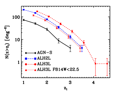
Figure 8: Number density of type-I AGN at $z>z_{i}$. The black solid line indicates the results for the AGN-S sample, which includes all the spectroscopically-known type-I AGN within the ALHAMBRA fields, the blue dot-dashed and red dashed lines for the ALH2L and ALH3L catalogues, respectively, and the red dotted line for the objects of the ALH3L catalogue with F814W $<22.5$. The error bars denote Poisson errors.

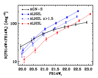
Figure 9: Number density of type-I AGN brighter than F814W_i. The colour coding is the same as in Fig. 8 for the AGN-S sample and the ALH2L and ALH3 catalogues. The blue dotted line indicates the results for the sources of the ALH2L catalogue with $z>1.5$. If we consider just objects with $z>1.5$ and F814W $<22.5$, the ALH2L catalogue contains $30\,\%$ more sources than the ALH3L catalogue.

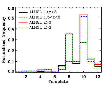
Figure 10: Distribution of the best-fitting templates for the ALH2L and ALH3L catalogues. The numbers in the x-axis correspond to the numbers in Table 2 and Fig. 6. In general, type-I AGN at $z<3$ prefer the template 8 and at $z>3$ the template 10.

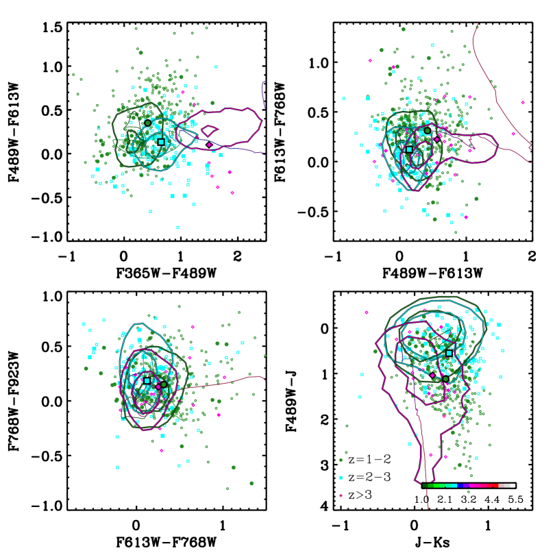
Figure 11: Colour-colour diagrams for the ALH2L catalogue. Only objects with photometric errors smaller than 0.2 mag in the bands shown are used to generate each panel. The colour of the symbols and lines indicates the redshift of the sources, as stated in the legend. Filled (open) symbols denote ALH2L objects that are (not) in common with the AGN-S sample, and big symbols indicate the median colours for all the objects at a certain redshift. Contours outline the colour loci of quasars from the SDSS-DR12 Quasar catalogue (top-left, top-right, and bottom-left panels) and the SDSS-DR6 Quasar catalogue with a counterpart in UKIDSS-LAS (bottom right panel), where the inner contours encloses the $0.5\,\%$ of the sample and the outer contour the $3\,\%$. From the top-left to bottom-right, for the SDSS quasars we show $g-r$ vs $u-g$, $r-i$ vs $g-r$, $i-z$ vs $r-i$, $g-J$ vs $J-K_{s}$. Narrow lines display the evolution of the colours of the template pl_QSOH as a function of $z$.

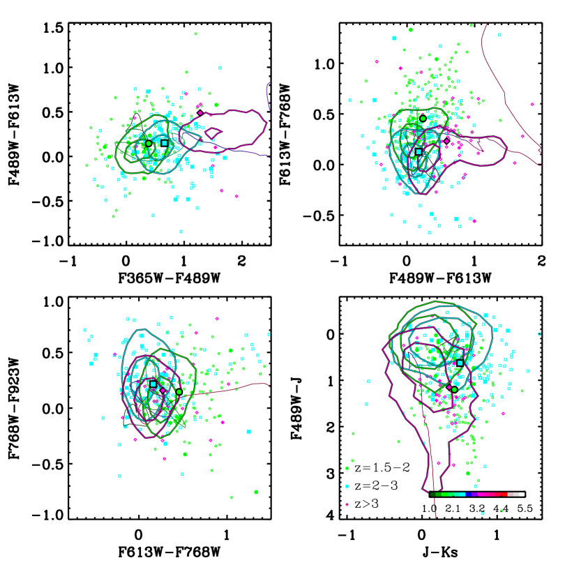
Figure 12: Colour-colour diagrams for the ALH3L catalogue. We employ the same colour coding as in Fig. 11.

4.1 Properties of the ALH2L and ALH3L catalogues

In this section we show the magnitudes, redshifts, best-fitting templates, and colours of the objects of the ALH2L and ALH3L catalogues.

To compute the number density of the ALH2L and ALH3L catalogues we need the effective area of the ALHAMBRA survey. To obtain it, we employ a mask generated by Arnalte-Mur et al. (2014) that excludes low exposure time areas, obvious defects in the images, and circular regions around saturated stars. After applying this mask, the effective area of the ALHAMBRA survey is $2.38\,\text{deg}^{2}$. We apply the same mask to the ALH2L and ALH3L catalogues, finding 498 and 419 objects within the mask, respectively, which correspond to a surface number density of $\simeq 209\,\text{deg}^{-2}$ and $\simeq 176\,\text{deg}^{-2}$. In Fig. 8 we display the number density of both catalogues as a function of redshift. The blue dot-dashed and red dashed lines indicate the number density for the ALH2L and ALH3L catalogues, respectively, and the black line does so for the AGN-S sample, which includes all the spectroscopically-known type-I AGN within the ALHAMBRA fields. As there are not obvious gaps in the redshift distribution of the ALH2L and ALH3L catalogues, we conclude that ELDAR uniformly identifies type-I AGN as a function of redshift. This is thanks to the continuity of the ALHAMBRA medium-bands. Non-contiguous bands would introduce gaps in the redshift distribution due to emission lines falling in between them.

In Fig. 8 we also show the number density for the objects of the ALH3L catalogue with F814W $<22.5$. As we can see, the 2- and 3-lines modes of ELDAR approximately detect the same number of type-I AGN at $z>2$ with F814W $<22.5$. The main strength of the first is that it allows to detect more objects than the second at $z<2$, whereas the best virtue of the 3-lines mode is that it allows to robustly confirm type-I AGN at lower SNR.

In Fig. 9 we display the number density of type-I AGN for the AGN-S sample and for the ALH2L and ALH3L catalogues as a function of the F814W magnitude. The number of sources detected by ELDAR grows like a power law up to the magnitude limit of the catalogues (F814W $=22.5$ and F814W $=23$ for the ALH2L and ALH3L catalogues, respectively); however, for the AGN-S sample it increases more slowly at F814W $>21$. Consenquently, given that that the contamination from galaxies and stars for the ALH2L and ALH3L catalogues is low (see §4.2), the approach of ELDAR is the most effective way of detecting faint type-I AGN in multi-filter surveys.

In Fig. 9 we can also see that for sources at $z>1.5$ and with F814W $<22.5$, the number of objects in the ALH2L catalogue is $30\,\%$ greater than in the ALH3L catalogue. We will discuss the completeness of both catalogues in §4.2.

In Fig. 10 we display the best-fitting template solution for the ALH2L and ALH3L catalogues as a function of $z$. In general, the distribution of templates for both catalogues is very similar, where the $35\,\%$ and $25\,\%$ of the sources at $z<3$ prefer the templates 8 and 10, and the $50\,\%$ of the objects at $z>3$ the template 10. The template 8 presents the SED of a high luminosity quasar and the number 10 depicts the SED of a synthetic quasar whose continuum emission follows a power law. We also find that the $85\,\%$ of the sources of the ALH2L and ALH3L catalogues are fitted by templates with low extinction ($E(B-V)<0.2$), in agreement with the fact we are targeting unobscured type-I AGN.

In an attempt to investigate whether the sources that ELDAR confirms as type-I are the same kind of objects as the AGN that spectroscopic surveys confirm, which are usually preselected using colour-colour diagrams, in Fig. 11 and 12 we display four colour-colour diagrams for the sources of the ALH2L and ALH3L catalogues, respectively, and SDSS quasars. For the SDSS quasars we show their broad-band SDSS colours, while for our ALHAMBRA objects we use the medium-bands colours closest to each broad-band SDSS colour. In the figures, the symbols indicate the colours of individual ALHAMBRA sources and the contours denote the colour loci of spectroscopically confirmed quasars from the SDSS-DR12 Quasar catalogue (Pâris et al., 2017) (top-left, top-right, and bottom-left panels) and the SDSS-DR6 Quasar catalogue with counterparts in the United Kingdom Infrared Telescope Infrared Deep Sky Survey Large Area Survey (UKIDSS-LAS) (Peth et al., 2011) (bottom right panel). Narrow-lines show the colours of the pl_QSOH template as a function of $z$. The average colours of the ALH2L and ALH3L samples are consistent with the colours of quasars observed after broad-band target selection. The larger colour distribution of the ALH2L and ALH3L samples (partially due to the fact that medium-bands are more sensitive to spectral features) indicates that our method is able to select objects with broader colour ranges. On the other hand, at $z<2$ the median colours of the objects of the ALH2L and ALH3L catalogues are displaced with respect to the centre of the SDSS contours. This is because SDSS does not systematically target quasars at $z<2.15$.

We conclude that ELDAR is not only able to select and characterise the typical quasars selected by broad-band surveys, but it has the potential of detecting a broader range of quasar types.

Figure 13: Redshift and F814W magnitude distribution for the GAL-S, AGN-S and AGN-X samples. We employ these samples to asses, respectively, the galaxy contamination, redshift precision, and completeness of the ALH2L and ALH3L catalogues.

4.2 Quality of the ALH2L and ALH3L catalogues

In order to asses the quality of the ALH2L and ALH3L catalogues, we need samples of spectroscopically-known type-I AGN and galaxies within the ALHAMBRA fields. We will employ the AGN-S sample (see §3.3) and two new samples: the first consists of X-ray selected type-I AGN in the ALHAMBRA COSMOS field (a sub-sample of the AGN-S sample). The second includes galaxies within the same ALHAMBRA field. We name them AGN-X and GAL-S, respectively.

We separate X-ray selected AGN to generate the AGN-X sample because X-ray selection produces complete samples of type-I AGN (Brandt & Hasinger, 2005) and thus, we can use the AGN-X sample to robustly estimate the completeness of the ALH2L and ALH3L catalogues. In addition, X-ray selected AGN catalogues have a low contamination from galaxies and stars (Lehmer et al., 2012; Stern et al., 2012). This catalogue is composed of 105 sources with F814W $<23$.

To obtain the GAL-S sample we match the objects from the DR2 of the zCOSMOS $10$k-bright spectroscopic sample (Lilly et al., 2009, zCOSMOS hereafter) with secure redshift (flags 3.x and 4.x) and the ALHAMBRA sources with F814W $<23$. zCOSMOS includes randomly selected galaxies with F814W $<22.5$ at $z_{\rm spec}<1.5$ in the COSMOS field, where the sampling rate is $\simeq 0.35$ in the area in common with the ALHAMBRA survey. Following the same procedure as for the AGN-S sample to do the match, we find a total of 1051 sources.

In Fig. 13 we display the magnitude and redshift distribution for the objects of the GAL-S, AGN-S, and AGN-X samples. In the following sections we will employ them to explore, respectively, the galaxy contamination, redshift precision, and completeness produced by the 2- and 3-lines modes of ELDAR. The results of this analysis are summarised in Table 3.

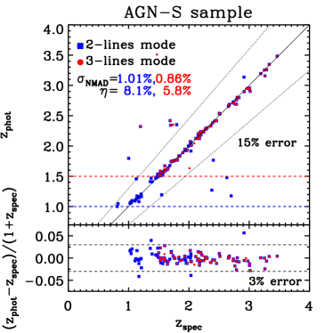
Figure 14: Comparison between photometric and spectroscopic redshifts for the AGN-S sample using the 2- and 3-lines modes of ELDAR. Blue squares and red circles denote objects identified by the 2- and 3-lines modes. The solid line indicates the $1:1$ relation, the dotted lines the threshold between good redshift solutions and outliers, and the blue (red) dashed line the redshift cut-off for the 2-lines (3-lines) mode. The normalised median absolute deviation, $\sigma_{\rm NMAD}$, and the fraction of outliers, $\eta$, are in blue and red for the 2- and 3-lines modes, respectivey. The bottom panel shows a measurement of the photo-$z$ accuracy for each source. Dashed lines indicate $3\,\%$ errors.

4.2.1 Redshift precision

We define the fraction of redshift outliers in a sample, $\eta$, as the percentage of objects with catastrophic redshift solutions for which $|z_{\rm spec}-z_{\rm phot}|>0.15\,(1+z_{\rm spec})$. We estimate this fraction for the ALH2L and ALH3L catalogues by applying the 2- and 3-lines modes of ELDAR to the AGN-S sample, respectively. We find that the fraction of outliers is a bit larger for the ALH2L catalogue, $\eta=8.1\,\%$, than for the ALH3L catalogue, $\eta=5.8\,\%$. This is because the larger the number of lines required to confirm an object, the lower is the probability for this object to be an outlier. These outliers are caused by a degeneracy between pairs of AGN emission lines, such as {C III], Mg II]} at $z=1.2$ and {Ly $\alpha$, C III]} at $z=2.3$, and {C IV, C III]} at $z=1.7$ and {Ly $\alpha$, C IV} at $z=2.4$. We show the ALHAMBRA photometric data of some of these outliers in Appendix A.

To compute the redshift precision for the catalogues, we employ the normalised median absolute deviation, $\sigma_{\rm NMAD}$, defined by Hoaglin et al. (1983) as

$$\sigma_{\rm NMAD}=1.48\;\text{median}\left(\frac{|z_{\rm phot}-z_{\rm spec}|}{1+z_{\rm spec}}\right).$$ (6)

We use $\sigma_{\rm NMAD}$ because it is designed to be less sensitive to redshift outliers than the standard deviation of photometric and spectroscopic redshifts. In a distribution without redshift outliers they would have the same value. Applying the 2- and 3-lines modes to the AGN-S sample, we obtain a redshift precision of $\sigma_{\rm NMAD}=1.01\,\%$ and $\sigma_{\rm NMAD}=0.86\,\%$, respectively. Therefore, the precision reached for type-I AGN using the 3-lines mode of ELDAR is even greater that the one achieved for galaxies and type-I AGN in other ALHAMBRA studies, see M14 and Matute et al. (2012), respectively.

Table 3: Results for the AGN-S, AGN-X, and GAL-S samples using the ELDAR’s 2- and 3-lines modes.

Sample	Mode	Compl. $(\%)$	$\sigma_{\rm NMAD}(\%)$	$\eta(\%)$
AGN-S	2-lines	71.7	1.01	8.1
	3-lines	65.2	0.86	5.8
AGN-X	2-lines	73.3	1.15	6.8
	3-lines	66.7	0.91	0.0
Sample	Mode	Galaxies confirmed as AGN
GAL-S	2-lines	4 (31 %)
	3-lines	1 (9 %)

Notes. Bold numbers indicate the estimated redshift precision, completeness, and galaxy contamination for the ALH2L and ALH3L catalogues. The galaxy contamination is extrapolated from the results for the GAL-S sample assuming that the ALHAMBRA COSMOS field is representative for all the ALHAMBRA fields.

In Fig. 14 we show the comparison between the spectroscopic and photometric redshifts of the sources of the AGN-S sample, where the photo-$z$s are computed using the 2- and 3-lines modes of ELDAR. The two modes produce precise results ($\sigma_{\rm NMAD}\leq 1\,\%$) with a fraction of outlier smaller than $10\,\%$. The results are particularly good at $z>2$, where we do not find any outlier for the 3-lines mode. In the bottom panel of Fig. 14 we display relative precision of the photo-$z$s produced by ELDAR. We find that it is greater than $3\,\%$ for $86\,\%$ and $93\,\%$ of the sources using the 2- and 3-lines mode, respectively, which shows that ELDAR produces accurate photo-$z$s for most of the sources.

In Table 4 we gather the redshift precision and outlier fraction for several X-rays selected samples (references in the caption). Most of the sources of the Cardamone et al. (2010); Luo et al. (2010); Hsu et al. (2014) samples are AGN whose SED is dominated by the host galaxy, and thus the photo-$z$ of these objects are straightforward to compute because the $4\,000\,{\rm\AA}$ break is visible. On the other hand, the Salvato et al. (2009, 2011); Fotopoulou et al. (2012); Matute et al. (2012) samples mostly contains type-I AGN. All these surveys, but the Lockman Hole area, which only has broad-band filters, have broad-, medium-, and narrow-band filters. As a consequence, the Lockman Hole sample is the one with the lowest redshift precision and the highest fraction of outliers. In this work, using the AGN-S sample, we obtain the best results in terms of redshift precision, which is because of the contiguous coverage of the optical range by the 20 medium-band filters of ALHAMBRA. Although the fraction of outliers that we obtain is not the lowest one, we want to highlight that the AGN-S sample is not X-ray selected. If we apply our methodology just to the AGN-X sample, we find no outliers using the 3-lines mode of ELDAR.

In Appendix Appendix B: Dependence of the results on the criteria adopted in ELDAR we study the redshift precision as a function of magnitude, redshift, and the value of the ELDAR free parameters.

Table 4: Redshift precision and fraction of outliers for different AGN/quasar catalogues.

Ref.	Bands	Depth	$\sigma_{\rm NMAD}(\%)$	$\eta(\%)$
$(a)$	30	$i^{*}_{AB}<22.5$	1.2	6.3
$(b)$	32	$R<26$	1.2	12.0
$(c)$	42	$R<26$	5.9	8.6
$(d)$	31	$i^{*}_{AB}<22.5$	1.1	5.1
$(e)$	21	$R_{c}<22.5$	8.4	21.4
$(f)$	23	$m_{678}<23.5$	0.9	12.3
$(g)$	50	$R<23$	1.1	4.2
$(h)$	23	F814W $<22.5$	1.01	8.1
$(i)$	23	F814W $<23$	0.86	5.8

Notes. $(a)$ XMM-Newton-COSMOS (QSOV sample, Salvato et al., 2009). $(b)$ The Multiwavelength Survey by Yale-Chile (X-ray sources, Cardamone et al., 2010). $(c)$ Chandra Deep Field-South (X-ray sources, Luo et al., 2010). $(d)$ XMM-Newton- and Chandra-COSMOS (QSOV sample, Salvato et al., 2011). $(e)$ Lockman Hole area (QSOV sample, Fotopoulou et al., 2012) $(f)$ ALHAMBRA (Matute et al., 2012). $(g)$ Extended Chandra Deep Field South (X-ray sources, Hsu et al., 2014). $(h)$ ALH2L catalogue (this work). $(i)$ ALH3L catalogue (this work).

4.2.2 Contamination from galaxies and stars

Because of their large number density and emission lines, star-forming galaxies are potentially the largest sample of objects that may be incorrectly classified as type-I AGN by ELDAR. This is because most stellar types do not have broad emission lines like type-I AGN. We will estimate the galaxy contamination in the ALH2L and ALH3L catalogues by applying the 2- and 3-lines modes of ELDAR to the GAL-S sample, where this sample allows us to estimate the galaxy contamination up to F814W $=22.5$.

Figure 15: Object of the GAL-S sample at $z_{\rm spec}=0.17$ that it is classified as type-I AGN by the 2- and 3-lines modes of ELDAR at $z_{\rm phot}=1.76$. This source is confirmed by ELDAR because there is a degeneracy between the triplet {[O II], [O III], H $\alpha$} at $z=0.17$ and the triplet {C IV, C III], Mg II} at $z=1.76$.

After applying the 2- and 3-lines modes of ELDAR to the $1\,051$ galaxies of the GAL-S sample, we end up with a total of 4 and 1 objects wrongly classified as type-I AGN, respectively. All of them show clear emission lines, have values of Stellarity $>0.6$, and are at $z_{\rm spec}<0.35$. In addition, we have visually inspected their spectra to confirm that they are low-$z$ star-forming galaxies. In Fig. 15 we show the only galaxy of the GAL-S sample that it is wrongly classified as type-I AGN by both the 2- and 3-lines modes. It is a point-like object (Stellarity $=0.95$) at $z_{\rm spec}=0.17$. This source is confirmed by our methodology because there is a degeneracy between the triplet {[O II], [O III], H $\alpha$} at $z=0.17$ and the triplet {C IV, C III], Mg II} at $z=1.76$. The other galaxies that are wrongly classified at type-I AGN by the 2-lines mode are objects for which there is a degeneracy between pairs of galaxy and AGN emission lines. None of them is confirmed due to spurious lines. This source of contamination is avoided because of the optimally selected value of $\sigma_{\rm line}$ for the 2- and 3-lines modes.

The effective area of the ALHAMBRA COSMOS field is $0.203\,\text{deg}^{2}$, which is $8.5\,\%$ of the total effective area of the ALHAMBRA survey, $2.38\,\text{deg}^{2}$. To compute the galaxy contamination for the ALH2L and ALH3L catalogues, we will assume that the ALHAMBRA COSMOS field is representative for the rest of the ALHAMBRA fields. As the sampling rate for zCOSMOS is $\simeq 0.35$ within the ALHAMBRA COSMOS field and $87\,\%$ of the galaxies at $z_{\rm spec}<0.35$ has secure redshifts, we estimate a galaxy contamination of 154 objects for the ALH2L catalogue and 38 for the ALH3L catalogue. This corresponds to a galaxy contamination of $31\,\%$ for the first and $9\,\%$ for the second. On the other hand, we expect the galaxy contamination at $z>2$ to be zero because ELDAR assigns photo-$z$ smaller than $z_{\rm phot}=2$ to the 4 galaxies wrongly classified as type-I AGN.

In Appendix Appendix B: Dependence of the results on the criteria adopted in ELDAR we study the galaxy contamination as a function of magnitude, redshift, and the value of the ELDAR free parameters.

We do not explore the contamination from stars because we already reject all the sources best-fitted by stellar templates and because normal stellar types do not show emission lines with large EWs. It is possible that stellar types with a very blue SED, e.g. O, A, and B, could be best-fitted by AGN templates; however, they would be rejected during the spectro-photometric step because they do not present emission lines with EWs large enough to be detected in ALHAMBRA. Another source of contamination could be Wolf-Rayet stars since they present broad emission lines of ionised helium, carbon, and nitrogen. Nevertheless, the predicted total number of Wolf-Rayet stars in our region of the galaxy is smaller than $1\,600$ (van der Hucht, 2001), and thus this kind of stars cannot be an important source of contamination.

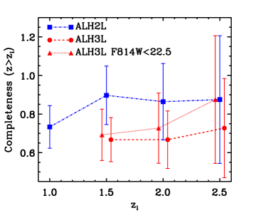
Figure 16: Completeness at $z>z_{i}$ for objects identified by ELDAR. The completeness is defined as the percentage of spectroscopically-known type-I AGN successfully confirmed by our method and it is estimated using just the objects of the AGN-X sample. For sources with $z>1.5$ the completeness is $\sim 90\,\%$ for the ALH2L catalogue.

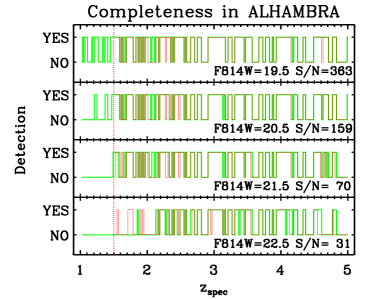
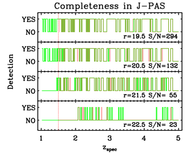
Figure 17: Detection of type-I AGN in ALHAMBRA and J-PAS using the 2- and 3-lines methods of ELDAR as a function of the magnitude in the detection band and the redshift of the mock source. The results are generated by convolving the synthetic template qso-0.2_84 with the ALHAMBRA and J-PAS filter systems. Green and red lines show the results for the 2-lines and 3-lines modes, respectively. There are bright objects which are not detected due to emission lines falling in between two bands. The number of confirmations for the faintest sources is smaller because the SNR is not large enough to detect all the AGN emission lines that ELDAR looks for.

4.2.3 Completeness

To estimate the completeness of the ALH2L and ALH3L catalogues, we apply the 2- and 3-lines modes of ELDAR to the AGN-X sample. We employ this sample because, as we explained before, X-ray selection produces largely complete samples of type-I AGN. We find a completeness of $73\,\%$ for the first (44 objects) and $67\,\%$ for the second (34 sources). Of the objects that the 2-lines mode does not classify as type-I AGN, $88\,\%$ of them have PDZ$(z_{\rm spec})<0.5$. We check that we do not obtain PDZ$(z_{\rm spec})>0.5$ for them including in LePHARE all the AGN templates from Salvato et al. (2009, 2011) and from the LePHARE distribution. For the 3-lines mode we find that $60\,\%$ of the objects not confirmed as type-I AGN have PDZ $(z_{\rm spec})<0.5$. The rest of them are rejected because ELDAR does not detect at least 3 AGN emission lines in their photometry. It is the consequence of objects for which some of their emission lines have a EW smaller than values listed in Table 1, and thus the ALHAMBRA bands are not narrow enough to confirm them. We also check that no source of the AGN-X sample is best-fitted by a stellar template in the first step of ELDAR.

In Fig. 16 we display the completeness of the ALH2L and ALH3L catalogues as a function of $z$. For the ALH2L catalogue the completeness grows from $z=1$ ($\simeq 70\,\%$) to $z=1.5$ ($\simeq 90\,\%$), and for higher redshifts it remains fairly constant. For the ALH3L catalogue the completeness is largely independent of $z$ and it is $\simeq 70\,\%$. For objects of the ALH3L catalogue with F814W $<22.5$, we can see that at $z=2.5$ the completeness is the same as for sources of the ALH2L catalogue at the same redshift. This confirms that the main strength of the 2-lines mode is to detect type-I AGN at low redshift (see Fig. 8).

We do not show the completeness at $z>2.5$ because there are only two objects in the AGN-X sample at higher redshifts. In Appendix Appendix B: Dependence of the results on the criteria adopted in ELDAR we use the AGN-S sample to study the completeness as a function of magnitude, redshift, and the value of the ELDAR free parameters. We employ the AGN-S because contains more objects that the AGN-X sample at high-$z$. We find that the completeness increases to $85\,\%$ and $77\,\%$ for objects of the ALH2L and ALH3L catalogues at $z>2$, respectively.

5 Forecasts for narrow band surveys

In this section we forecast the performance of ELDAR in surveys with narrower bands than the ALHAMBRA survey, as our method can be applied to any survey in which the bands are narrow enough to isolate AGN emission lines from the continuum.

There are several surveys that incorporate contiguous bands narrower than the ALHAMBRA bands, such as SHARDS (25 bands of FWHM $\simeq 170\,\rm{\AA}$), PAUS (40 bands of FWHM $\simeq 130\,\rm{\AA}$), and the upcoming J-PAS (54 bands of FWHM $\simeq 140\,\rm{\AA}$). As the data from all of these surveys is not publicly available yet, we decided to forecast the completeness and redshift precision for J-PAS because it has the greatest number of bands, and thus we expect to find the largest differences between the results for ALHAMBRA and for this survey.

To estimate the performance of ELDAR detecting type-I AGN in J-PAS and to make a fair comparison with ALHAMBRA, we generate AGN-mock data for the ALHAMBRA and J-PAS filter systems. In order to do that, we convolve the template qso-0.2_84 with both filter systems and we shift it in redshift between $z=1$ and $z=5$ using a redshift step of $\Delta z=0.02$. Then, we create 4 mock sources at each redshift imposing a magnitude of 19.5, 20.5, 21.5, and 22.5 in the detection band of ALHAMBRA and J-PAS, which are the F814W band for the first and the $r$ band for the second. We note that these magnitudes correspond to different SNR in the medium-/narrow-bands of these surveys, given their different magnitude limits. Next, we compute the error in each band using a empirical relation for ALHAMBRA mock data and the J-PAS exposure time calculator for J-PAS mock data (J. Varela, private communication). Finally, we apply the 2- and 3-lines modes of ELDAR to both samples, where the only modification that we include in ELDAR for J-PAS data is that we change the redshift step employed in LePHARE from 0.01 to 0.001. This is done because J-PAS includes narrower and more numerous contiguous bands than the ALHAMBRA survey, and thus we expect a higher redshift precision (Benítez et al., 2009).

In Fig. 17 we show the performance of ELDAR using ALHAMBRA and J-PAS data as a function of the redshift and magnitude of the source. At low-$z$, the gaps in the redshift distribution are caused by the blue and steep continuum emission of the qso-0.2_84 template, which makes more difficult to detect emission lines. This is even more important for mock sources dimmer than 21 mag., as none of them are confirmed by ELDAR. Nonetheless, as we can see in Fig. 9, at $z<1.5$ we detect plenty of ALHAMBRA sources with F814W $>21$. This is because the SED of real type-I AGN is not as steep as the continuum of the qso-0.2_84 template.

The no-detection of bright objects at $z>2$ in some redshift intervals is due to Ly $\alpha$ falling in between two bands. While this is an important issue for ALHAMBRA, it gets alleviated in the case of J-PAS. This is because if we introduce a redshift-dependent continuum or we model it using the bands which are adjacent to the band where Ly $\alpha$ falls, we could confirm these sources. The smaller number of detections as we decrease the brightness of the sources is because the SNR required to detect some of the AGN lines gathered in Table 1 is not large enough.

Using the 3-lines mode of ELDAR, we achieve a redshift precision of $\sigma_{\rm NMAD}=0.48\,\%$ and $\sigma_{\rm NMAD}=0.21\,\%$ for mock ALHAMBRA and J-PAS data, respectively. As we get $\sigma_{\rm NMAD}=0.86\,\%$ for real ALHAMBRA data (see Table 3), we forecast a precision of $\sigma_{\rm NMAD}=0.38\,\%$ for J-PAS, which is similar to the one expected for J-PAS galaxies (Benítez et al., 2014).

6 Summary and conclusions

The emergence of multi-filter surveys such as COSMOS, SHARDS, the ongoing PAUS, and the upcoming J-PAS, open the possibility of developing new techniques to fully exploit these data that lie at the interface between photometry and spectroscopy. In this work we presented ELDAR, a new method that enables the secure identification of unobscured AGN and the precise computation of their redshifts. Using as input only the multi-band information for each observed source, ELDAR takes advantage of the low-resolution spectroscopic nature of the data to look for AGN emission lines, thus allowing an unambiguous AGN identification. With this approach, ELDAR offers a new method to confirm AGN in multi-filter surveys without the need, for example, of spectroscopic follow-up or X-ray observations.

We started by presenting the main characteristics of ELDAR, which consists of two main steps. In the first we apply the template fitting code LePHARE to all the point-like objects that we want to classify, rejecting most of the stars and producing a redshift probability distribution function for every extragalactic object. In the second step, we confirm the AGN candidates by looking for typical AGN emission lines in each extragalactic object. This allows us to generate samples of AGN with a very low contamination from galaxies.

To test the performance of ELDAR we applied it to the publicly available data from the ALHAMBRA survey, which covered an effective area of $2.38\,\text{deg}^{2}$ of the northern sky with 20 contiguous medium-bands of FWHM $\simeq 300\,\rm{\AA}$. Given the bandwidth of the ALHAMBRA filters, we tuned our code to detect only type-I AGN. These objects, in fact, are characterised by emission lines that can dominate the ALHAMBRA band in which they fall thanks to their large equivalent width. Then, we defined two different configurations of ELDAR, where the first prioritises completeness and requires the detection of at least 2 AGN emission lines, while the second prioritises purity and requires the detection of 3 lines. After the pre-selection using LePHARE, we blindly ran both configurations of ELDAR on the ALHAMBRA data, ending up with two AGN samples of 585 and 494 sources, respectively (ALH2L and ALH3L catalogues). The ALH2L sample covers the redshift range $1<z<5.5$ and it is limited to F814W $<22.5$. The ALH3L catalogue spans the range $1.5<z<5.5$, and contains objects up to F814W $<23$. Approximately $80\,\%$ of the sources of our catalogues were lacking a spectroscopic identification and redshift estimation. We make publicly available the ALH2L and ALH3L catalogues, where we provide both the ALHAMBRA photometric data and our redshift estimate.

To characterise the properties of the ALH2L and ALH3L catalogues we ran the 2- and 3-lines configurations of ELDAR on samples of spectroscopically-known type-I AGN and galaxies in the ALHAMBRA fields, estimating, for the two catalogues, a completeness of $73\,\%$ and $67\,\%$, a redshift precision of $\sigma_{\rm NMAD}=1.01\,\%$ and $\sigma_{\rm NMAD}=0.86\,\%$, and a galaxy contamination of $31\,\%$ and $9\,\%$, respectively. We obtain the best results for sources at $z>2$, as the Ly-alpha line enters the spectral coverage of ALHAMBRA. At those redshifts, the completeness increases to $85\,\%$ and $77\,\%$ for the two-modes, and we no longer find galaxy contamination.

Thanks to the depth of the ALHAMBRA data, we have been able to push the detection of type-I AGN to faint sources which are typically not accessible by spectroscopic surveys. We would like to stress that ELDAR, when applied to multi-filter surveys such as ALHAMBRA, does not require additional data from X-ray, radio, nor variability studies to confirm type-I AGN.

Finally, we forecast the performance of ELDAR in surveys with narrower bands than ALHAMBRA. We analysed the particular case of the upcoming J-PAS survey, which will cover thousands of square degrees of the northern sky with 54 narrow-bands of FWHM $\simeq 140\,\rm{\AA}$. We generated mock J-PAS and ALHAMBRA data using a typical AGN SED template. Then, applying ELDAR to the mock data, we estimated that J-PAS can reach a significantly better redshift precision than ALHAMBRA thanks to the larger number of bands.

To conclude, we point out that ELDAR can be further improved: for example, the first obvious step will be a more detailed modelling of the AGN continuum emission. Also, we plan to optimise the code for the detection of narrow AGN emission lines for narrow-band surveys such as PAUS and J-PAS. With such improvements, we expect ELDAR to perform even better in terms of completeness and redshift precision for range of active galaxies.

 

Figure 18: ELDAR results for spectroscopically-known type-I AGN. We show illustrative examples of objects correctly classifies as type-I AGN, redshift outliers, objects for which ELDAR does not detect all the available lines, and the only source of the AGN-S sample misclassified as a star. In all panels, arrows point to the bands where AGN emission lines are confirmed. Top-left panel: low-$z$ AGN ($z_{\rm spec}=1.80$) correctly classified as type-I AGN by the 2- and 3-lines modes of ELDAR. Top-right panel: high-$z$ AGN ($z_{\rm spec}=3.52$) correctly classified as type-I AGN by the 3-lines mode of ELDAR (it is not classified as AGN by the 2-lines mode because it is fainter that the magnitude limit for this mode, F814W $22.5$). Medium-left panel: low-$z$ AGN ($z_{\rm spec}=1.83$) classified as type-I AGN just by the 2-lines mode of ELDAR. This is because the 3-lines mode does not detect C III] at $5404\rm{\AA}$. Medium-right panel: high-$z$ AGN ($z_{\rm spec}=2.91$) only classified as type-I AGN by the 2-lines mode of ELDAR. The 3-lines mode does not detect C IV at $6407\rm{\AA}$ nor C III] at $7895\rm{\AA}$. Bottom-left panel: low-$z$ at $z_{\rm spec}=1.69$ classified as AGN by the 2- and 3-lines modes of ELDAR at $z_{\rm phot}=2.42$. This is because the the pair {Ly $\alpha$, C IV} at $z=2.42$ is degenerated with the position of the pair {C IV, C III]} at $z=1.69$. Bottom-right panel: only source of the AGN-S sample that it is best-fitted by a stellar template. We cannot see any clear emission line in the ALHAMBRA data.

Appendix A: AGN examples

To illustrate the objects of the AGN-S sample that ELDAR confirms and rejects and why it does so, in Fig. 18 we display the SED of multiple sources and we discuss whether they fulfil all ELDAR’s criteria or not. In the panels we use arrows to point to the bands where ELDAR detects AGN emission lines. We indicate the name of the lines according to $z_{\rm spec}$. In the top-left panel we show an object of the AGN-S sample at $z_{\rm spec}=1.80$. After applying the 2- and 3-lines modes of ELDAR, we find that it is correctly classified as AGN by both. This is because our method detects C IV in the 3rd band, C III] in the 5th band, and Mg II in the 14th band. In addition, the redshift that ELDAR assigns to this object, $z_{\rm phot}=1.77$, is compatible with its spectroscopic redshift, $z_{\rm phot}=1.78$. In top-right panel we display an object of the AGN-S sample at $z_{\rm spec}=3.52$ that is classified as type-I AGN by the 3-lines mode of ELDAR. This is because our method detects the complex O VI+Ly $\beta$ in the 4th band, Ly $\alpha$ in the 8th band, and C III] in the 17th band. On the other hand, the line C IV is not detected because it falls between the 12th and 13th bands. According to $z_{\rm spec}$, the central wavelength of the lines Ly $\alpha$ and C IV should be very close to the central wavelength of the 7th and 12th band, respectively. However, the first falls between the 7th and 8th band and the second between the 12th and 13th band. This is because AGN emission lines may be shifted with respect to their rest-frame wavelength and/or have anisotropic profiles (see Vanden Berk et al., 2001), where these effects can modify the band where they fall. As a consequence, the photometric redshift computed for this source, $z_{\rm phot}=3.63$, is $\simeq 3\,\%$ greater than its spectroscopic redshift.

In the medium-left panel we plot a source of the AGN-S sample at $z_{\rm spec}=1.83$. This object is classified as AGN just by the 2-lines mode of ELDAR. This is because our method detects C IV in the 3rd band, Mg II in the 15th band, but not C III] because it falls between the 6th and 7th bands. The photometric redshift computed by ELDAR, $z_{\rm phot}=1.83$, is the same as its spectroscopic redshift, $z_{\rm spec}=1.83$. In the medium-right panel we show the only object of the AGN-S sub-sample with $z_{\rm spec}>2.75$ not confirmed as type-I AGN by the 3-lines mode. However, it is classified as type-I AGN by the 2-lines mode. This is because our code does not detect C IV, which should fall in the 10th band, nor C III], which should fall in the 15th band. It is the consequence of the ALHAMBRA bands not been narrow enough for detecting these lines. The lack of these lines causes the computed photometric redshift, $z_{\rm phot}=3.14$, to be $\simeq 8\,\%$ greater than the spectroscopic redshift for this object, $z_{\rm spec}=2.91$. In these two panels we have shown a low-$z$ and a high-$z$ spectroscopically-known object that are not classified as type-I AGN by the 3-lines mode of ELDAR. Objects like these ones explain why the 3-lines mode has a lower completeness than the 2-lines mode. In the following, we will show some examples of spectroscopically-known objects for which ELDAR produces catastrophic redshift solutions.

In the bottom-left panel we display a source of the AGN-S sample at $z_{\rm spec}=1.69$ classified as type-I AGN by the 2- and 3-lines modes at $z_{\rm phot}=2.42$. Thus, this object is an outlier according to our definition (see §4.2.1). This is because i) PDZ$(z_{\rm spec})<0.5$ and ii) there is a degeneracy between the pair {Ly $\alpha$, C IV} at $z=2.42$ and the pair {C IV, C III]} at $z=1.69$. This source is also confirmed by the 3-lines mode because C III] is confused with a spurious line detected in the 9th band. In the bottom-right panel we display the only object of the AGN-S sample best-fitted by a stellar template. This object is at $z_{\rm spec}=1.52$ and it does not show any clear emission lines. The best-fitting AGN templates has a $\chi^{2}$ more than twice the $\chi^{2}$ of the best-fitting stellar templates. Even if this object is not best-fitted by an AGN template, it will not be confirmed as type-I AGN because ELDAR does not detect any AGN emission lines. No objects from the AGN-X sample are best-fitted by stellar templates.

Appendix B: Dependence of the results on the criteria adopted in ELDAR

In §2 and §3.3 we introduced multiple parameters in the configuration of ELDAR. In this section we show the dependence of the results for the objects of the AGN-S and GAL-S samples on these criteria. In all the tables we underline the results for the fiducial configuration of ELDAR.

Table 5: Results for the AGN-S and GAL-S samples as a function of the PDZ cut-off.

PDZ	Mode	Compl.$(\%)$	$\sigma_{\rm NMAD}(\%)$	$\eta(\%)$	Galaxies
0.90	2-lines	71.1	1.00	7.3	4
	3-lines	64.4	0.86	5.9	1
0.50	2-lines	71.7	1.01	8.1	4
	3-lines	65.2	0.86	5.8	1
0.01	2-lines	72.2	1.02	8.8	4
	3-lines	66.7	0.92	6.8	1

Notes. Bold numbers denote fiducial values for the 2- and 3-lines modes of ELDAR.

We introduced a PDZ cut-off of 0.5 in ELDAR to reject redshift solutions for which the $\chi^{2}$ is very low. In Table 5 we gather the results for the AGN-S and GAL-S samples using different values of the PDZ cut-off. The quality of the ALH2L and ALH3L catalogues is largely independent of the value of this parameter. This is because most of the objects with F814W $<22.5$ have only one peak in their PDZ with PDZ $>0.5$.

Table 6: Results for the AGN-S and GAL-S samples as a function of the Ly $\alpha$ criterion.

Ly $\alpha$	Mode	Compl.$(\%)$	$\sigma_{\rm NMAD}(\%)$	$\eta(\%)$	Galaxies
1.25	2-lines	67.3	1.00	6.8	4
	3-lines	60.6	0.86	3.8	1
0.75	2-lines	71.7	1.01	8.1	4
	3-lines	65.2	0.86	5.8	1
0.25	2-lines	72.2	1.00	7.2	4
	3-lines	65.9	0.86	5.7	1

Another criterion that we included in ELDAR is that the flux in the band where the Ly $\alpha$ line falls has to be $75\,\%$ greater than the flux in the rest of the bands. In Table 6 we present the results for the AGN-S and GAL-S using different percentages. We find that increasing this percentage the completeness is reduced.

Table 7: Results for the AGN-S and GAL-S samples as a function of the line acceptance criterion.

$\sigma_{\rm line}$	Mode	Compl.$(\%)$	$\sigma_{\rm NMAD}(\%)$	$\eta(\%)$	Galaxies
0.50	2-lines	78.6	1.10	9.6	13
0.75		77.4	1.07	8.2	11
1.00		75.1	1.06	7.7	7
1.25		75.1	1.05	8.5	4
1.50		71.7	1.01	8.1	4
1.75		69.4	0.98	8.3	1
0.50	3-lines	67.4	0.96	5.6	1
0.75		65.2	0.86	5.8	1
1.00		61.4	0.96	6.2	1
1.25		56.8	0.86	5.7	1
1.50		49.2	0.86	4.9	0
1.75		44.7	0.86	5.1	0

Notes. $\sigma_{\rm line}$ indicates the minimum number of $\sigma$s that we require to confirm an emission lines.

We set different requirements to confirm emission lines for the 2- and 3-lines modes. For the 2-lines mode we established a stricter acceptance criterion than for the 3-lines mode to reduce possible galaxy contamination. In Table 7 we display the results for the AGN-S and GAL-S samples using different acceptance criteria. We find that the smaller is the value of $\sigma_{\rm line}$, the higher is the completeness and the galaxy contamination. Moreover, the galaxy contamination strongly grows by reducing $\mathcal{N}$, and thus $\sigma_{\rm line}$ has to be carefully chosen depending on $\mathcal{N}$.

Table 8: Results for the AGN-S and GAL-S samples as a function of $z_{\rm min}$.

$z_{\rm min}$	Mode	Compl.$(\%)$	$\sigma_{\rm NMAD}(\%)$	$\eta(\%)$	Galaxies
1.0	2-lines	71.7	1.01	8.1	4
	3-lines	-	-	-	-
1.5	2-lines	79.8	0.87	6.3	3
	3-lines	65.2	0.86	5.8	1
2.0	2-lines	84.8	0.92	7.1	0
	3-lines	77.0	0.97	8.8	0
2.5	2-lines	80.0	0.91	0.0	0
	3-lines	75.7	0.86	4.0	0

Notes. The 3-lines mode is not defined at $z=1$ because there are less than 3 AGN emission lines that ELDAR looks for within the ALHAMBRA wavelength coverage.

The condition of detecting at least 2 or 3 AGN emission lines to confirm objects sets a minimum redshift, $z_{\rm min}$, for the sources. In order to check whether the ELDAR’s performance depends on the redshift of the sources, we apply the 2- and 3-lines modes to the AGN-S and GAL-S samples using different values of $z_{\rm min}$. In Table 8 we gather the results. We find that the completeness increases as a function of the redshift, and the galaxy contamination decreases. Moreover, the redshift precision is largely independent of $z_{\rm min}$.

Table 9: Results for the AGN-S and GAL-S samples as a function of the magnitude limit in the detection band, F814W.

F814W	Mode	Compl.$(\%)$	$\sigma_{\rm NMAD}(\%)$	$\eta(\%)$	Galaxies
21.5	2-lines	73.8	0.98	5.6	2
	3-lines	65.8	0.77	1.8	1
22.0	2-lines	70.3	0.97	5.9	3
	3-lines	62.9	0.78	1.6	1
22.5	2-lines	71.7	1.01	8.1	4
	3-lines	64.7	0.86	3.9	1
23.0	2-lines	70.0	1.06	9.8	4
	3-lines	65.2	0.86	5.8	1

Finally, we address the dependence of the results on the magnitude limit. In Table 9 we summarize the results for the AGN-S and GAL-S samples using the 2- and 3-lines modes. For both modes, the completeness does not depend strongly on the magnitude limit; however, the redshift precision grows for brighter objects and the galaxy contamination decreases.

Appendix C: Description of the ALH2L and ALH3L catalogues

The catalogues ALH2L and ALH3L are available as binary ASCII tables. They are documented in an accessory README file (column, bytes, format, units, label, description) and it is also shown in §4.

Notes on the catalogue columns:

1	The identification number of each object. The format is ALHXLYYY, where the value of X is 2 and 3 for the ALH2L and ALH3L catalogues, respectively, and YYY is the number of the object. The IDs are ranked according to $z_{\rm phot}$.
2 - 4	J2000 coordinates (right ascension, sign of the declination, and declination). The astrometry is from ALHAMBRA.
5	ELDAR redshift solution.
6	Flag that indicates whether an object is inside the ALHAMBRA mask (1) or not (0).
7	Index of the AGN template that best-fit the data.
8 - 9	Extinction law and colour excess of the extragalactic template that best-fit the data. The extinction is 0 for templates without extinction and 1 for the Calzetti et al. (2000) extinction law, 2 for the Allen (1976) extinction law, 3 for the Prevot et al. (1984) extinction law, and 4 for the Fitzpatrick (1986) extinction law.
10 - 11	PSF-magnitude and uncertainty in the F814W band.
12	Stellarity parameter of SExtractor. In ALHAMBRA it does not provide accurate results for objects with F814W $>23$.
13 - 50	PSF-magnitude and uncertainty in ALHAMBRA medium-bands.
51 - 56	PSF-magnitude and uncertainty in ALHAMBRA infrared broad-bands.
57 - 74	ALHAMBRA band where the AGN emission lines of Table 1 fall. We set this value to 99 for no detections and to 0 for lines outside the wavelength range. For detected lines we also include the SNR in the band where they fall, and the significance with which they are detected, ${\rm S}_{\rm lin}$, defined as:
	$${\rm S}_{\rm lin}={\rm min}\left\{\begin{aligned} &\frac{F_{\rm cen}-F_{\rm blue}}{S_{\rm cen}}-\sigma_{\rm line},\\ &\frac{F_{\rm cen}-F_{\rm red}}{S_{\rm cen}}-\sigma_{\rm line},\\ &\frac{F_{\rm cen}-F_{\rm blue}}{S_{\rm cen}}-\sigma_{\rm line}\frac{S_{\rm blue}}{S_{\rm cen}},\\ &\frac{F_{\rm cen}-F_{\rm red}}{S_{\rm cen}}-\sigma_{\rm line}\frac{S_{\rm red}}{S_{\rm cen}}.\\ \end{aligned}\right.$$ (7)

Table 10: Byte-by-byte description of the ALH2L and ALH3L catalogues.

Column	Bytes	Format	Units	Label	Description
1	1-8	A8	–	ID	Identification number
2	10-17	F8.4	deg	RA	Right Ascension J2000 [0, 360]
3	19	A1	–	DE-	Declination J2000 (sign)
4	20-26	F7.4	deg	DEC	Declination J2000 [-90, 90]
5	28-32	F5.3	–	Z	Photometric redshift
6	34	I1	–	MASK	Mask [0 outside, 1 inside]
7	36-37	I2	–	TEMP	Best-fit extragalactic template
8	39-42	F4.2	–	EXTB	Best-fit colour excess
9	44-49	F6.3	mag	F814W	F814W magnitude
10	51-55	F5.3	mag	eF814W	F814W uncertainty
11	57-60	F4.2	–	STELL	SExtractor Stellarity parameter
					[1 point-like, 0 extended]
12	62-68	F7.3	mag	F365W	F365W magnitude
13	70-76	F7.3	mag	eF365W	F365W uncertainty
14	78-84	F7.3	mag	F396W	F396W magnitude
15	86-92	F7.3	mag	eF396W	F396W uncertainty
16	94-100	F7.3	mag	F427W	F427W magnitude
17	102-108	F7.3	mag	eF427W	F427W uncertainty
18	110-116	F7.3	mag	F458W	F458W magnitude
19	118-124	F7.3	mag	eF458W	F458W uncertainty
20	126-132	F7.3	mag	F489W	F489W magnitude
21	134-140	F7.3	mag	eF489W	F489W uncertainty
22	142-148	F7.3	mag	F520W	F520W magnitude
23	150-156	F7.3	mag	eF520W	F520W uncertainty
24	158-164	F7.3	mag	F551W	F551W magnitude
25	166-172	F7.3	mag	eF551W	F551W uncertainty
26	174-180	F7.3	mag	F582W	F582W magnitude
27	182-188	F7.3	mag	eF582W	F582W uncertainty
28	190-196	F7.3	mag	F613W	F613W magnitude
29	198-204	F7.3	mag	eF613W	F613W uncertainty
30	206-212	F7.3	mag	F644W	F644W magnitude
31	214-220	F7.3	mag	eF644W	F644W uncertainty
32	222-228	F7.3	mag	F675W	F675W magnitude
33	230-236	F7.3	mag	eF675W	F675W uncertainty
34	238-244	F7.3	mag	F706W	F706W magnitude
35	246-252	F7.3	mag	eF706W	F706W uncertainty
36	254-260	F7.3	mag	F737W	F737W magnitude
37	262-268	F7.3	mag	eF737W	F737W uncertainty
38	270-276	F7.3	mag	F768W	F768W magnitude
39	278-284	F7.3	mag	eF768W	F768W uncertainty
40	286-292	F7.3	mag	F799W	F799W magnitude
41	294-300	F7.3	mag	eF799W	F799W uncertainty
42	302-308	F7.3	mag	F830W	F830W magnitude
43	310-316	F7.3	mag	eF830W	F830W uncertainty
44	318-324	F7.3	mag	F861W	F861W magnitude
45	326-332	F7.3	mag	eF861W	F861W uncertainty
46	334-340	F7.3	mag	F892W	F892W magnitude
47	342-348	F7.3	mag	eF892W	F892W uncertainty
48	350-356	F7.3	mag	F923W	F923W magnitude
49	358-364	F7.3	mag	eF923W	F923W uncertainty
50	366-372	F7.3	mag	F954W	F954W magnitude
51	374-380	F7.3	mag	eF954W	F954W uncertainty
52	382-388	F7.3	mag	J	J magnitude
53	390-396	F7.3	mag	eJ	J uncertainty
54	398-404	F7.3	mag	H	H magnitude
55	406-412	F7.3	mag	eH	H uncertainty
56	414-420	F7.3	mag	Ks	$K_{s}$ magnitude
57	422-428	F7.3	mag	eKs	$K_{s}$ uncertainty
58	430-431	I2	–	LINE1	Band where the O VI+Ly $\beta$
					complex is detected [2,19]
59	433-438	F6.3	–	SNLINE1	$\log_{10}({\rm SNR})$ in the band where
					the O VI+Ly $\beta$ complex is detected
60	440-445	F6.3	–	SLINE1	$\log_{10}({\rm S}_{\rm lin})$ in the band where
					the O VI+Ly $\beta$ complex is detected
61	447-448	I2	–	LINE2	Band where the Ly $\alpha$ line
					is detected [2,19]
62	450-455	F6.3	–	SNLINE2	$\log_{10}({\rm SNR})$ in the band where
					the Ly $\alpha$ line is detected
63	457-462	F6.3	–	SLINE2	$\log_{10}({\rm S}_{\rm lin})$ in the band where
					the Ly $\alpha$ line is detected
64	464-469	I2	–	LINE3	Band where the Si IV+O IV]
					complex is detected [2,19]
65	471-476	F6.3	–	SNLINE3	$\log_{10}({\rm SNR})$ in the band where
					the Si IV+O IV] complex is detected
66	478-479	F6.3	–	SLINE3	$\log_{10}({\rm S}_{\rm lin})$ in the band where
					the Si IV+O IV] complex is detected
67	481-482	I2	–	LINE4	Band where the C IV line
					is detected [2,19]
68	484-489	F6.3	–	SNLINE4	$\log_{10}({\rm SNR})$ in the band where
					the C IV line is detected
69	491-496	F6.3	–	SLINE4	$\log_{10}({\rm S}_{\rm lin})$ in the band where
					the C IV line is detected
70	498-499	I2	–	LINE5	Band where the C III] line
					is detected [2,19]
71	501-506	F6.3	–	SNLINE5	$\log_{10}({\rm SNR})$ in the band where
					the C III] line is detected
72	508-513	F6.3	–	SLINE5	$\log_{10}({\rm S}_{\rm lin})$ in the band where
					the C III] line is detected
73	515-516	I2	–	LINE6	Band where the Mg II line
					is detected [2,19]
74	518-523	F6.3	–	SNLINE6	$\log_{10}({\rm SNR})$ in the band where
					the Mg II line is detected
75	525-530	F6.3	–	SLINE6	$\log_{10}({\rm S}_{\rm lin})$ in the band where
					the Mg II line is detected

Table 10: *

References

- Allen (1976) Allen C. W., 1976, Astrophysical Quantities
- Antonucci (1993) Antonucci R., 1993, ARA&A, 31, 473
- Aparicio Villegas et al. (2010) Aparicio Villegas T., Alfaro E. J., et al., 2010, AJ, 139, 1242
- Arnalte-Mur et al. (2014) Arnalte-Mur P., et al., 2014, MNRAS, 441, 1783
- Arnouts et al. (1999) Arnouts S., Cristiani S., Moscardini L., Matarrese S., Lucchin F., Fontana A., Giallongo E., 1999, MNRAS, 310, 540
- Barger et al. (2003) Barger A. J., Cowie L. L., Capak P., Alexander D. M., Bauer F. E., Fernandez E., Brandt W. N., Garmire G. P., Hornschemeier A. E., 2003, AJ, 126, 632
- Benítez et al. (2009) Benítez N., et al., 2009, ApJ, 692, L5
- Benítez et al. (2014) Benítez N., et al., 2014, ArXiv e-prints, arXiv:1403.5237
- Bertin & Arnouts (1996) Bertin E., Arnouts S., 1996, A&AS, 117, 393
- Bixler et al. (1991) Bixler J. V., Bowyer S., Laget M., 1991, A&A, 250, 370
- Bohlin et al. (1995) Bohlin R. C., Colina L., Finley D. S., 1995, AJ, 110, 1316
- Bolzonella et al. (2000) Bolzonella M., Miralles J.-M., Pelló R., 2000, A&A, 363, 476
- Brandt & Hasinger (2005) Brandt W. N., Hasinger G., 2005, ARA&A, 43, 827
- Brusa et al. (2003) Brusa M., Comastri A., Mignoli M., Fiore F., Ciliegi P., Vignali C., Severgnini P., Cocchia F., La Franca F., Matt G., Perola G. C., Maiolino R., Baldi A., Molendi S., 2003, A&A, 409, 65
- Busca et al. (2013) Busca N. G., et al., 2013, A&A, 552, A96
- Calzetti et al. (2000) Calzetti D., Armus L., Bohlin R. C., Kinney A. L., Koornneef J., Storchi-Bergmann T., 2000, ApJ, 533, 682
- Cardamone et al. (2010) Cardamone C. N., van Dokkum P. G., Urry C. M., Taniguchi Y., Gawiser E., Brammer G., Taylor E., Damen M., Treister E., Cobb B. E., Bond N., Schawinski K., Lira P., Murayama T., Saito T., Sumikawa K., 2010, ApJS, 189, 270
- Chabrier et al. (2000) Chabrier G., Baraffe I., Allard F., Hauschildt P., 2000, ApJ, 542, 464
- Civano et al. (2016) Civano F., Marchesi S., Comastri A., et al., 2016, ApJ, 819, 62
- Dawson et al. (2016) Dawson K. S., Kneib J.-P., Percival W. J., Alam S., Albareti F. D., Anderson S. F., et al., 2016, 151, 44
- Fitzpatrick (1986) Fitzpatrick E. L., 1986, AJ, 92, 1068
- Flesch (2015) Flesch E. W., 2015, PASA, 32, e010
- Fotopoulou et al. (2012) Fotopoulou S., Salvato M., Hasinger G., Rovilos E., Brusa M., Egami E., Lutz D., Burwitz V., Henry J. P., Huang J. H., Rigopoulou D., Vaccari M., 2012, ApJS, 198, 1
- Gallerani et al. (2010) Gallerani S., Maiolino R., Juarez Y., Nagao T., Marconi A., Bianchi S., Schneider R., Mannucci F., Oliva T., Willott C. J., Jiang L., Fan X., 2010, A&A, 523, A85
- Gavignaud et al. (2006) Gavignaud I., et al., 2006, A&A, 457, 79
- Gebhardt et al. (2000) Gebhardt K., Bender R., Bower G., Dressler A., Faber S. M., Filippenko A. V., Green R., Grillmair C., Ho L. C., Kormendy J., Lauer T. R., Magorrian J., Pinkney J., Richstone D., Tremaine S., 2000, ApJ, 539, L13
- Heckman & Best (2014) Heckman T. M., Best P. N., 2014, ARA&A, 52, 589
- Hoaglin et al. (1983) Hoaglin D. C., Mosteller F., Tukey J. W., 1983, Understanding robust and exploratory data anlysis
- Hsu et al. (2014) Hsu L.-T., et al., 2014, ApJ, 796, 60
- Ilbert et al. (2009) Ilbert O., et al., 2009, ApJ, 690, 1236
- Jahnke & Macciò (2011) Jahnke K., Macciò A. V., 2011, ApJ, 734, 92
- Kormendy & Richstone (1995) Kormendy J., Richstone D., 1995, ARA&A, 33, 581
- Lacy et al. (2004) Lacy M., et al., 2004, ApJS, 154, 166
- Lehmer et al. (2012) Lehmer B. D., Xue Y. Q., Brandt W. N., Alexander D. M., Bauer F. E., Brusa M., Comastri A., Gilli R., Hornschemeier A. E., Luo B., Paolillo M., Ptak A., Shemmer O., Schneider D. P., Tozzi P., Vignali C., 2012, ApJ, 752, 46
- Lilly et al. (2009) Lilly S. J., et al., 2009, ApJS, 184, 218
- Luo et al. (2010) Luo B., Brandt W. N., Xue Y. Q., Brusa M., Alexander D. M., Bauer F. E., Comastri A., Koekemoer A., Lehmer B. D., Mainieri V., Rafferty D. A., Schneider D. P., Silverman J. D., Vignali C., 2010, ApJS, 187, 560
- Marchesi et al. (2016) Marchesi S., Lanzuisi G., Civano F., Iwasawa K., Suh H., Comastri A., Zamorani G., Allevato V., Griffiths R., Miyaji T., Ranalli P., Salvato M., Schawinski K., Silverman J., Treister E., Urry C. M., Vignali C., 2016, ApJ, 830, 100
- Martí et al. (2014) Martí P., Miquel R., Castander F. J., Gaztañaga E., Eriksen M., Sánchez C., 2014, MNRAS, 442, 92
- Matthews & Sandage (1963) Matthews T. A., Sandage A. R., 1963, ApJ, 138, 30
- Matute et al. (2012) Matute I., et al., 2012, A&A, 542, A20
- Matute et al. (2013) Matute I., et al., 2013, A&A, 557, A78
- Moles et al. (2008) Moles M., et al., 2008, AJ, 136, 1325
- Molino et al. (2014) Molino A., et al., 2014, MNRAS, 441, 2891
- Mortlock et al. (2011) Mortlock D. J., Warren S. J., Venemans B. P., Patel M., Hewett P. C., McMahon R. G., Simpson C., Theuns T., Gonzáles-Solares E. A., Adamson A., Dye S., Hambly N. C., Hirst P., Irwin M. J., Kuiper E., Lawrence A., Röttgering H. J. A., 2011, Nature, 474, 616
- Osterbrock (1991) Osterbrock D. E., 1991, Reports on Progress in Physics, 54, 579
- Pâris et al. (2017) Pâris I., et al., 2017, 597, A79
- Peng (2007) Peng C. Y., 2007, ApJ, 671, 1098
- Pérez-González & Cava (2013) Pérez-González P. G., Cava A., 2013, in Revista Mexicana de Astronomia y Astrofisica Conference Series Vol. 42 of Revista Mexicana de Astronomia y Astrofisica, vol. 27, SHARDS: Survey for High-z Absorption Red & Dead Sources. pp 55–57
- Peth et al. (2011) Peth M. A., Ross N. P., Schneider D. P., 2011, AJ, 141, 105
- Pickles (1998) Pickles A. J., 1998, PASP, 110, 863
- Planck Collaboration et al. (2016) Planck Collaboration Ade P. A. R., Aghanim N., Arnaud M., Ashdown M., Aumont J., Baccigalupi C., Banday A. J., Barreiro R. B., Bartlett J. G., et al., 2016, A&A, 594, A13
- Prevot et al. (1984) Prevot M. L., Lequeux J., Prevot L., Maurice E., Rocca-Volmerange B., 1984, A&A, 132, 389
- Risaliti & Lusso (2017) Risaliti G., Lusso E., 2017, Astronomische Nachrichten, 338, 329
- Salvato et al. (2009) Salvato M., et al., 2009, ApJ, 690, 1250
- Salvato et al. (2011) Salvato M., et al., 2011, ApJ, 742, 61
- Schmidt et al. (2010) Schmidt K. B., Marshall P. J., Rix H.-W., Jester S., Hennawi J. F., Dobler G., 2010, ApJ, 714, 1194
- Scoville et al. (2007) Scoville N., et al., 2007, ApJS, 172, 1
- Stern et al. (2012) Stern D., Assef R. J., Benford D. J., Blain A., Cutri R., Dey A., Eisenhardt P., Griffith R. L., Jarrett T. H., Lake S., Masci F., Petty S., Stanford S. A., Tsai C.-W., Wright E. L., Yan L., Harrison F., Madsen K., 2012, ApJ, 753, 30
- Telfer et al. (2002) Telfer R. C., Zheng W., Kriss G. A., Davidsen A. F., 2002, ApJ, 565, 773
- Urry & Padovani (1995) Urry C. M., Padovani P., 1995, PASP, 107, 803
- van der Hucht (2001) van der Hucht K. A., 2001, New A Rev., 45, 135
- Vanden Berk et al. (2001) Vanden Berk D. E., et al., 2001, AJ, 122, 549
- Wang et al. (2014) Wang J.-M., Du P., Hu C., Netzer H., Bai J.-M., Lu K.-X., Kaspi S., Qiu J., Li Y.-R., Wang F., SEAMBH Collaboration 2014, ApJ, 793, 108
- Watson et al. (2011) Watson D., Denney K. D., Vestergaard M., Davis T. M., 2011, ApJ, 740, L49
- White et al. (2000) White R. L., Becker R. H., Gregg M. D., Laurent-Muehleisen S. A., Brotherton M. S., Impey C. D., Petry C. E., Foltz C. B., Chaffee F. H., Richards G. T., Oegerle W. R., Helfand D. J., McMahon R. G., Cabanela J. E., 2000, ApJS, 126, 133
- Wolf et al. (2008) Wolf C., Hildebrandt H., Taylor E. N., Meisenheimer K., 2008, A&A, 492, 933
- Wolf et al. (2004) Wolf C., Meisenheimer K., Kleinheinrich M., Borch A., Dye S., Gray M., Wisotzki L., Bell E. F., Rix H.-W., Cimatti A., Hasinger G., Szokoly G., 2004, A&A, 421, 913
- Zhao et al. (2016) Zhao G.-B., Wang Y., Ross A. J., Shandera S., Percival W. J., et al., 2016, 457, 2377
1 Centro de Estudios de Física del Cosmos de Aragón, Plaza San Juan 1, Planta-3, 44001, Teruel, Spain.
2 Max-Planck Institut für extraterrestrische Physik, Postfach 1312, 85741 Garching bei München, Germany.
3 Instituto de Física de Cantabria (CSIC-UC), 39005 Santander, Spain.
4 Unidad Asociada Observatorio Astronómico (IFCA-UV), 46980 Patema, Spain.
5 Ethiopian Space Science and Technology Institute (ESSTI), Entoto Observatory and Research Center (EORC), Astronomy and Astrophysics Research Division, P.O. Box 33679, Addis Ababa, Ethiopia.
6 Instituto de Astrofísica de Andalucía (IAA-CSIC), Glorieta de la Astronomía s/n, 18008 Granada, Spain.
7 APC, AstroParticule et Cosmologie, Universitè Paris Diderot, CNRS/IN2P3, CEA/Irfu, Observatoire de Paris, Sorbonne Paris Citè, 10, rue Alice Domon et Lèonie Duquet, 75205 Paris Cedez 13, France.
8 Observatori Astronòmic, Universitat de València, c/ Catedràtic José Beltraán 2, 46980 Patema, Spain.
9 Departament d’Astronomia i Astrofísica, Universitat de València, 46100 Burjassot, Spain.
10 Instituto de Astrofísica e Ciências do Espao̧, Universidade de Lisboa, OAL, Tapada da Ajuda, PT1349-018 Lisbon, Portugal.
11 Departamento de Física Matemática, Instituto de Física, Universidade de São Paulo, CP 66318, CEP 05314-970 São Paulo, Brazil.
12 Instituto de Astrofísica de Andalucía, CSIC, Apdo 3004, 18080 Granada, Spain.