Bounds for OPE coefficients on the Regge trajectory

Abstract

We consider the Regge limit of the CFT correlation functions $\langle{\cal J}{\cal J}{\cal O}{\cal O}\rangle$ and $\langle TT{\cal O}{\cal O}\rangle$, where ${\cal J}$ is a vector current, $T$ is the stress tensor and ${\cal O}$ is some scalar operator. These correlation functions are related by a type of Fourier transform to the AdS phase shift of the dual 2-to-2 scattering process. AdS unitarity was conjectured some time ago to be positivity of the imaginary part of this bulk phase shift. This condition was recently proved using purely CFT arguments. For large $N$ CFTs we further expand on these ideas, by considering the phase shift in the Regge limit, which is dominated by the leading Regge pole with spin $j(\nu)$, where $\nu$ is a spectral parameter. We compute the phase shift as a function of the bulk impact parameter, and then use AdS unitarity to impose bounds on the analytically continued OPE coefficients $C_{{\cal J}{\cal J}j(\nu)}$ and $C_{TTj(\nu)}$ that describe the coupling to the leading Regge trajectory of the current ${\cal J}$ and stress tensor $T$. AdS unitarity implies that the OPE coefficients associated to non-minimal couplings of the bulk theory vanish at the intercept value $\nu=0$, for any CFT. Focusing on the case of large gap theories, this result can be used to show that the physical OPE coefficients $C_{{\cal J}{\cal J}T}$ and $C_{TTT}$, associated to non-minimal bulk couplings, scale with the gap $\Delta_{g}$ as $\Delta_{g}^{-2}$ or $\Delta_{g}^{-4}$. Also, looking directly at the unitarity condition imposed at the OPE coefficients $C_{{\cal J}{\cal J}T}$ and $C_{TTT}$ results precisely in the known conformal collider bounds, giving a new CFT derivation of these bounds. We finish with remarks on finite $N$ theories and show directly in the CFT that the spin function $j(\nu)$ is convex, extending this property to the continuation to complex spin.

1 Introduction

Correlation functions of local operators in Conformal Field Theory (CFT) are determined by a set of numbers - scaling dimensions and Operator Product Expansion (OPE) coefficients - known as the CFT data. These numbers are not arbitrary because they must be compatible with OPE associativity, unitarity and the existence of a local stress energy tensor. It would be very useful to find an organizing principle for the CFT data. In this paper, we explore the idea of Regge trajectories as organizing principle.

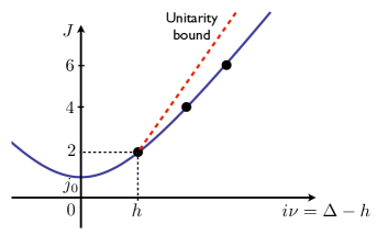
Different kinematical limits focus on different subsets of the CFT data. One such example is the light-cone limit Fitzpatrick:2012yx ; Komargodski:2012ek ; Alday:2016njk ; Alday:2016jfr which has recently been used to prove the conformal collider bounds Hofman:2008ar and the CEMZ bounds Camanho:2014apa on OPE coefficients of conserved currents and stress-tensors from the CFT side Hartman:2015lfa ; arXiv:1511.08025 ; arXiv:1603.03771 ; Hartman:2016lgu ; Afkhami-Jeddi:2016ntf . Here we study the Regge limit of CFT four-point correlators Cornalba:2007fs ; Costa:2012cb , which are dominated by the leading Regge trajectory, i.e. the set of operators of lowest dimension $\Delta(J)$ for each even spin $J$. We focus on correlators for which the exchanged Regge trajectories have the vacuum quantum numbers. In this case the leading trajectory encodes a lot of interesting physics, since its first operator is the stress tensor. In particular, in Nachtmann:1973mr ; Komargodski:2012ek it was shown that this trajectory is convex, as depicted in figure 1. The argument involves a deep inelastic scattering thought experiment in a gapped phase obtained by deforming the CFT with a relevant operator. However, it has been shown recently Caron-Huot:2017vep , that this trajectory admits a continuation into complex spin $J$. Using this new result we shall be able to prove the convexity directly in the CFT, showing also that this property extends to the continuation to non-integer spin. As we shall review, it is this continuation that controls the Regge limit of the four-point function. In particular, the high energy growth of the correlator is determined by the value of the intercept $j_{0}$ shown in figure 1 and defined by $\Delta(j_{0})=d/2$.

Figure 1: Shape of the leading Regge trajectory $J=j(\nu)$ with vacuum quantum numbers in a CFT. The dimension of operators $\Delta$ is related to the spectral parameter $\nu$ by $\Delta=h+i\nu$ where $h=d/2$. The function $j(\nu)$ is even and convex. The minimum (for imaginary $\nu$) is the intercept $j(0)\equiv j_{0}$.

The leading Regge trajectory also plays a central role in holographic CFTs. In this context, we assume a large $N$ expansion and consider the leading trajectory of single-trace operators. In the gravity limit, the absence of light higher spin fields in the bulk implies a large gap in the operator dimensions, i.e. that $\Delta_{g}\equiv\Delta(J=4)\gg 1$. Therefore, large $N$ and large $\Delta_{g}$ are necessary conditions for the emergence of a local bulk dual. It is also natural to conjecture that these conditions are sufficient for bulk locality Heemskerk:2009pn . There has been a significant amount of work testing this conjecture. More concretely, we would like to prove that CFTs with large $N$ and large $\Delta_{g}$ have other expected universal properties of gravitational theories in AdS. One such property is that tree-level high energy scattering is dominated by graviton exchange. In CFT language, this means that the intercept $j_{0}\to 2$ as $\Delta_{g}\to\infty$. Convexity of the single-trace leading Regge trajectory would automatically imply this result. However, the convexity property that we prove in appendix F only applies to the exact leading Regge trajectory of the finite $N$ theory. This is further discussed in our concluding remarks.

Another expected property of tree-level high energy scattering in gravitational theories is that the higher derivative couplings to the graviton are suppressed by the mass scale of higher spinning particles. In the gravitational context, this follows from causality Camanho:2014apa . Therefore, in the CFT language, we should be able to prove that some OPE coefficients are suppressed by powers of $\Delta_{g}\gg 1$. Consider for example the three graviton coupling. The bulk effective action can be written schematically as

$$\frac{1}{16\pi G_{N}}\int d^{d+1}x\sqrt{g}\left[\frac{d(d-1)}{\ell^{2}}+\mathcal{R}+\alpha_{2}\ell^{2}\mathcal{R}^{2}+\alpha_{4}\ell^{4}\mathcal{R}^{3}+\dots\right],$$ (1)

where $\ell$ is the radius of the AdS solution when the higher derivative dimensionless couplings $\alpha_{2}$ and $\alpha_{4}$ vanish. The authors of Camanho:2014apa showed that causality implies the effective field theory scaling

$$\alpha_{2}\ell^{2}\sim\frac{1}{m_{g}^{2}}\,,\qquad\qquad\alpha_{4}\ell^{4}\sim\frac{1}{m_{g}^{4}}\,,$$ (2)

where $m_{g}$ is the mass of higher spin particles. In CFT language, this translates into a statement about the three point function of the stress tensor. In any CFT, this can be written as

$$\langle TTT\rangle=\langle TTT\rangle_{\mathcal{R}}+\alpha_{2}\langle TTT\rangle_{\mathcal{R}^{2}}+\alpha_{4}\langle TTT\rangle_{\mathcal{R}^{3}}\,,$$ (3)

where each term corresponds to a different tensor structure. We would like to prove that

$$C_{TTT}^{(2)}\sim\alpha_{2}\sim\frac{1}{\Delta_{g}^{2}}\,,\qquad\qquad C_{TTT}^{(3)}\sim\alpha_{4}\sim\frac{1}{\Delta_{g}^{4}}\,,$$ (4)

where $C_{TTT}^{(i)}$ are OPE coefficients. This has been argued in Hartman:2016lgu ; Afkhami-Jeddi:2016ntf ; Kulaxizi:2017ixa ; Li:2017lmh . Here we provide another argument based on unitarity of the bulk phase shift conjectured a while ago in Cornalba:2008sp and recently proved in Kulaxizi:2017ixa .

In section 2, we review Conformal Regge Theory and generalize it for the four-point function of two stress tensors and two scalar operators. Section 3 reviews the recent proof Kulaxizi:2017ixa of the AdS unitarity condition and determines subleading contributions, which allow us to analyze the validity of the condition. In section 4 the AdS unitarity condition is used to derive bounds on OPE coefficients of two currents (or two stress tensors) and operators of the leading Regge trajectory. The phase shift is computed using a saddle point approximation, where the location $\nu_{0}$ of the saddle depends on the AdS impact parameter $L$. By varying $L$ one can move the saddle point to different interesting points on the Regge trajectory, starting from the intercept at $\nu_{0}=0$, to the stress-tensor at $\nu_{0}=\pm ih$ and to the spin 4 operator $\mathcal{O}_{J=4}$ at $\nu_{0}=\pm i(\Delta_{g}-h)$. The resulting bounds are summarized in table 1. In particular, with mild assumptions on the behaviour of OPE coefficients in the large gap limit, we are able to show (4). We conclude in section 5 with some remarks on finite $N$ CFTs. The appendices contain technical details and a proof of the convexity of the leading Regge trajectory.

$\nu_{0}$	$\ J\$	$L$	bounds on $C_{TTj(\nu_{0})}^{(i)}$	$\Delta_{g}$
0	$j_{0}$	0	$C_{TTj(0)}^{(2)}=C_{TTj(0)}^{(3)}=0$	any
$\pm ih$	$2$	$\sim\ln S$	conformal collider bounds Hofman:2008ar	any
$\pm i(\Delta_{g}-h)$	$4$	$\sim\ln S$	$\frac{C_{TT\mathcal{O}_{\!J=4}}^{(2)}}{C_{TT\mathcal{O}_{\!J=4}}^{(1)}}\lesssim\frac{1}{\Delta_{g}^{2}},\ \frac{C_{TT\mathcal{O}_{\!J=4}}^{(3)}}{C_{TT\mathcal{O}_{\!J=4}}^{(1)}}\lesssim\frac{1}{\Delta_{g}^{4}}$	$\Delta_{g}\gg 1$ and flat space limit

Table 1: Summary of bounds on the leading Regge trajectory. For theories with a large $\Delta_{g}$, we show that the bounds at $\nu_{0}=0$ imply (4). In order to derive the bounds at $\nu_{0}=\pm i(\Delta_{g}-h)$, given in (144), we have to impose in addition to large $\Delta_{g}$ the stronger condition that there is a well defined flat space limit. Analogous bounds are obtained for the OPE coefficient with two conserved currents.

2 Conformal Regge theory

In this section we will review the main formulae for the Regge limit of CFT correlators Cornalba:2007fs ; Costa:2012cb . For the sake of clarity, we start with the case of correlators of scalar operators, leaving the complications of distinct tensor structures that arise for external spinning operators for subsequent subsections. In order to prepare the ground to derive non-trivial bounds for OPE coefficients we will finish this section with the case of two vector currents and two scalars already derived in Cornalba:2009ax , and then present the extension to the case of two stress tensors and two scalars.

2.1 Regge kinematics

We start with the four-point correlation function $A(y_{i})=\big{\langle}{\cal O}_{1}(y_{1}){\cal O}_{2}(y_{2}){\cal O}_{3}(y_{3}){\cal O}_{4}(y_{4})\big{\rangle}$, of four scalar operators of dimension $\Delta_{i}$ placed at $y_{i}$. We will be interested in the case ${\cal O}_{1}={\cal O}_{2}$ and ${\cal O}_{3}={\cal O}_{4}$. In this case we can write

$$A(y_{i})=\frac{{\cal A}({z,\bar{z}})}{(y_{12})^{2\Delta_{1}}(y_{34})^{2\Delta_{3}}}\,,$$ (5)

where $z,\bar{z}$ are the usual cross ratios

$$z\bar{z}=\frac{y_{12}y_{34}}{y_{13}y_{24}}\,,\ \ \ \ \ \ \ \ \ \ (1-z)(1-\bar{z})=\frac{y_{14}y_{23}}{y_{13}y_{24}}\,.$$ (6)

We shall normalize the operators according to $\big{\langle}{\cal O}_{i}(y){\cal O}_{i}(0)\big{\rangle}=1/y^{2\Delta_{i}}$.

Figure 2: Regge kinematics requires $y_{13}^{2},y_{24}^{2}>0$ and $y_{14}^{2},y_{23}^{2}<0$. The left panel shows the Regge kinematics for $y_{12}^{2},y_{34}^{2}>0$, but that is not necessary since we may allow $y_{2}$ to cross the light cone of $y_{1}$ and $y_{4}$ the light cone of $y_{3}$. The right panel shows the path of the cross ratios $z,\bar{z}$ as we analytically continue from the Euclidean region to the Lorentzian one.

We wish to consider a CFT in $d$-dimensional Minkowski space $\mathbb{M}^{d}$ and study the Regge limit of the above correlation function. In light-cone coordinates $y=(y^{+},y^{-},y_{\perp})$, where $y_{\perp}$ is a point in transverse space $\mathbb{R}^{d-2}$, the Regge limit is defined by

$$y_{1}^{+}\rightarrow-\infty\,,\ \ \ \ \ \ y_{2}^{+}\rightarrow+\infty\,,\ \ \ \ \ \ y_{3}^{-}\rightarrow-\infty\,,\ \ \ \ \ \ y_{4}^{-}\rightarrow+\infty\,,\ \ \ \ \ \$$ (7)

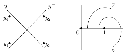
while keeping $y_{i}^{2}$ and $y_{i\perp}$ fixed. In particular we shall keep the causal relations $y_{14}^{2},y_{23}^{2}<0$ and all the other $y_{ij}^{2}>0$. This Lorentzian correlation function, with time ordered operators, is obtained by analytic continuation from the Euclidean one where $\bar{z}=z^{*}$ Cornalba:2006xk . With the above kinematics, the correct prescription is to fix $\bar{z}$ and rotate $z$ anti-clockwise around the branch point at $z=1$. In the Lorentzian sheet both $z$ and $\bar{z}$ are real. Figure 2 shows the kinematics and analytic continuation.

Figure 3: The CFT can be defined on the Lorentzian cylinder (left figure). By a conformal transformation one can move to a Poincaré patch, defining the theory on Minkowski space, that covers only a portion of the cylinder. The central Poincaré patch, where operator insertions are close to null infinity, is shown in blue. One may instead consider Poincaré patches whose origins, shown as white dots, are at null infinity of the central Poincaré patch. The operator ${\cal O}_{i}$ is then inserted very close to the origin of the Poincaré patch ${\cal P}_{i}$, where we use coordinates $x_{i}$. To visualize the different Poincaré patches it is convenient to open the cylinder (right figure). The red lines are identified in this picture.

A convenient parameterization of the correlation function considers a conformal transformation on each point, such that each point is close to the origin of a Poincaré patch. This can be done with the transformations

$$x_{i}=(x_{i}^{+},x_{i}^{-},x_{i\perp})=-\frac{1}{y_{i}^{+}}\left(1,y_{i}^{2},y_{i\perp}\right)\,,\ \ \ \ \ \ \ \ \ i=1,2\,,$$ (8)

$$x_{i}=(x_{i}^{+},x_{i}^{-},x_{i\perp})=-\frac{1}{y_{i}^{-}}\left(1,y_{i}^{2},y_{i\perp}\right)\,,\ \ \ \ \ \ \ \ \ i=3,4\,.$$ (9)

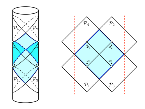
The Regge limit is now the limit $x_{i}\rightarrow 0$. Notice, however, that the operators are not close to each other, since the $x_{i}$ are close to the origin of distinct Poincaré patches. Figure 3 shows the different Poincaré patches, which cover a portion of the Lorentzian cylinder $\mathbb{R}\times S^{d-1}$ where we can define our theory. Note that this cylinder can be thought as belonging to the boundary of global AdS space, although our arguments are purely based in CFT. Studying the action of the conformal group on the different patches it is possible to show that, in the Regge limit, the correlation function can only depend on the combinations Cornalba:2009ax

$$x\approx x_{1}-x_{2}\,,\ \ \ \ \ \ \ \ \ \ \ \ \bar{x}\approx x_{3}-x_{4}\,.$$ (10)

Moreover, we can write the only two independent cross ratios

$$\sigma^{2}=x^{2}\bar{x}^{2}\,,\ \ \ \ \ \ \ \ \ \cosh\rho=-\frac{x\cdot\bar{x}}{|x||\bar{x}|}\,,$$ (11)

so that the Regge limit corresponds to sending $\sigma\rightarrow 0$ with $\rho$ fixed. Notice that these cross ratios are related to $z,\bar{z}$ by $z\bar{z}=x^{2}\bar{x}^{2}$ and $z+\bar{z}=-2x\cdot\bar{x}$.

Following the standard transformation for conformal primaries

$$\mathcal{O}(y)=\left|\frac{\partial x}{\partial y}\right|^{\frac{\Delta}{d}}\mathcal{O}(x)\ ,$$ (12)

the transformed correlation function $A(x_{i})=\big{\langle}{\cal O}_{1}(x_{1}){\cal O}_{2}(x_{2}){\cal O}_{3}(x_{3}){\cal O}_{4}(x_{4})\big{\rangle}$ is related to the original one by

$$A(y_{i})=(-y_{1}^{+}y_{2}^{+})^{-\Delta_{1}}(-y_{3}^{-}y_{4}^{-})^{-\Delta_{2}}\,A(x_{i})\,.$$ (13)

For example, for the disconnected part of the correlation function we have

$$\langle{\cal O}_{1}(x_{1}){\cal O}_{2}(x_{2})\rangle=\frac{1}{\left(-x^{2}+i\epsilon_{x}\right)^{\Delta_{1}}}\,,\ \ \ \ \ \ \langle{\cal O}_{3}(x_{3}){\cal O}_{4}(x_{4})\rangle=\frac{1}{\left(-\bar{x}^{2}+i\epsilon_{\bar{x}}\right)^{\Delta_{3}}}\,,$$ (14)

where we use the $i\epsilon$-prescription, $\epsilon_{x}=\epsilon\,{\rm sgn}\,x^{0}$ Cornalba:2006xk . Notice that each vector $x_{i}$ is defined with respect to its own Poincaré patch ${\cal P}_{i}$. Thus, although both $x$ and $\bar{x}$ are small vectors, these are two-point functions between points that are far apart but approaching the light-cone of each other. For time-like $x$, ${\cal O}_{1}$ and ${\cal O}_{2}$ are space-like related, while for space-like $x$ they are time-like related.

2.2 Conformal block expansion

We want to consider the expansion of the correlation function in terms of $t$-channel conformal blocks,

$$\mathcal{A}(z,\bar{z})=\sum_{k}C_{12k}C_{34k}\,G_{\Delta_{k},J_{k}}(z,\bar{z})\,,$$ (15)

where $C_{ijk}$ are the OPE coefficients and $G_{\Delta,J}(z,\bar{z})$ is the conformal block associated to the exchange of a primary of dimension $\Delta$ and spin $J$. For our purposes, it is more useful to consider the spectral representation Dobrev:1975ru ; Cornalba:2007fs ; Costa:2012cb

$$\mathcal{A}(z,\bar{z})=\sum_{J}\int_{-\infty}^{\infty}d\nu\,b_{J}\big{(}\nu^{2}\big{)}\,F_{\nu,J}(z,\bar{z})\,,$$ (16)

where

$$F_{\nu,J}(z,\bar{z})=\kappa_{\nu,J}\,G_{h+i\nu,J}(z,\bar{z})+\kappa_{-\nu,J}\,G_{h-i\nu,J}(z,\bar{z})\,,$$ (17)

is a sum of two conformal blocks with dimensions $h+i\nu$ and $h-i\nu$ (we use $h=d/2$ throughout the paper), with the normalization constant

$$\kappa_{\nu,J}=\frac{i\nu}{2\pi K_{h+i\nu,J}}\,.$$ (18)

The definition of the function $K_{\Delta,J}$ is given in equation (161) of appendix A. The two conformal blocks in (17) satisfy the same differential equation because they have the same Casimir eigenvalue. The second conformal block is usually called the shadow of the first (see for example SimmonsDuffin:2012uy for details). The basis of functions $F_{\nu,J}(z,\bar{z})$ forms a complete basis of single valued functions that satisfy the Casimir equation Caron-Huot:2017vep . They are therefore ideal to expand the Euclidean correlator ${\cal A}(z,\bar{z}=z^{*})$.

In order to reproduce, from the spectral representation (16), the contribution in (15) of a primary of dimension $\Delta$ and spin $J$ that appears in both OPEs $\mathcal{O}_{1}\mathcal{O}_{2}$ and $\mathcal{O}_{3}\mathcal{O}_{4}$, the partial amplitude $b_{J}(\nu^{2})$ must have poles of the form

$$\nu^{2}\to-(\Delta-h)^{2}\,,\qquad b_{J}\big{(}\nu^{2}\big{)}\approx\frac{r(\Delta,J)}{\nu^{2}+(\Delta-h)^{2}}\,,\qquad r(\Delta,J)=C_{12J}C_{34J}K_{\Delta,J}\,.$$ (19)

We remark that the function $\kappa_{\nu,J}$ has poles corresponding to the spin $J$ double traces of the type $\mathcal{O}_{1}\partial_{\mu_{1}}\dots\partial_{\mu_{J}}\partial^{2m}\mathcal{O}_{2}$ and $\mathcal{O}_{3}\partial_{\mu_{1}}\dots\partial_{\mu_{J}}\partial^{2m}\mathcal{O}_{4}$. This is tailored to the case of large $N$ AdS duals for which a $t$-channel tree level Witten diagram includes double trace exchanges DHoker:1999mic ; Cornalba:2006xm . For general CFTs these poles are canceled by zeros of the function $b_{J}(\nu^{2})$.

2.3 Regge theory

To consider the Regge theory we need to perform an analytic continuation of the conformal blocks above, corresponding to a Wick rotation from the Euclidean to the Lorentzian correlator. In terms of the cross ratios $z,{\bar{z}}$, we need to continue $z$ around $1$ counter clockwise with $\bar{z}$ held fixed. This computation is described in appendix A. The result is that after analytic continuation and in the limit $\sigma\rightarrow 0$ at fixed $\rho$, the function $F_{\nu,J}(z,\bar{z})$ is to leading order in $\sigma$ given by

$$F_{\nu,J}(z,\bar{z})\approx-i\pi^{h}4^{J}\sigma^{1-J}\gamma(\nu)\gamma(-\nu)\,\Omega_{i\nu}(\rho)\,,$$ (20)

where $\gamma(\nu)$, defined in (163), is a function with poles at the double trace operators and $\Omega_{i\nu}(\rho)$ is the harmonic function on hyperbolic space $H_{d-1}$ defined in (164). Note that due to the factor $\sigma^{1-J}$ exchanges of large spin contribute most to the Regge limit. This is the reason why we need to resum all exchanges of the leading Regge trajectory to get a sensible result. The first step is to rewrite (16) as follows

$$\mathcal{A}(z,\bar{z})=\sum_{J}\int d\nu\,b_{J}\big{(}\nu^{2}\big{)}\,\frac{1}{2}\left[F_{\nu,J}(z,\bar{z})+F_{\nu,J}\left(\frac{z}{z-1},\frac{\bar{z}}{\bar{z}-1}\right)\right]\,,$$ (21)

using the fact that only even spins contribute to the four-point function with $\mathcal{O}_{3}=\mathcal{O}_{4}$ and that $F_{\nu,J}\left(\frac{z}{z-1},\frac{\bar{z}}{\bar{z}-1}\right)=(-1)^{J}F_{\nu,J}(z,\bar{z})$. Notice that this transformation of the cross-ratios corresponds to the exchange $3\leftrightarrow 4$ (or $1\leftrightarrow 2$). Next we do the usual Sommerfeld-Watson transform to replace the sum over $J$ by an integral

$${\cal A}(z,\bar{z})=\int d\nu\int_{C}\frac{dJ}{2\pi i}\frac{\pi}{2\sin(\pi J)}\,b_{J}\big{(}\nu^{2}\big{)}\,\left[F_{\nu,J}(z,\bar{z})+F_{\nu,J}\left(\frac{z}{z-1},\frac{\bar{z}}{\bar{z}-1}\right)\right]\,.$$ (22)

Analytic continuation in the $J$-plane allows us to deform the $J$ contour picking the Regge pole with largest ${\rm Re}J$. In this step, we made the important assumptions that we can drop the contribution from $J=\infty$ and that the leading singularity is a Regge pole. More precisely the pole comes from expanding the denominator of the function (19) around $J\approx j(\nu)$

$$b_{J}(\nu^{2})\approx-\frac{j^{\prime}(\nu)\,r(\nu)}{2\nu\big{(}J-j(\nu)\big{)}}\,,$$ (23)

where $j(\nu)$ is the inverse function of $\Delta(J)$ defined by

$$\nu^{2}+\big{(}\Delta(j(\nu))-h\big{)}^{2}=0\,,$$ (24)

and we defined the function $r(\nu)$ obtained from the analytic continuation of the OPE coefficients that appear in the combination given in (19),

$$r(\nu)\equiv r\big{(}h\pm i\nu,j(\nu)\big{)}=C_{12j(\nu)}C_{34j(\nu)}K_{h\pm i\nu,j(\nu)}\,.$$ (25)

That this analytic continuation is well defined was only recently proved in Caron-Huot:2017vep . Using (20), we conclude that the contribution of this Regge pole is

$${\cal A}(\sigma,\rho)=\int_{-\infty}^{\infty}d\nu\,\alpha(\nu)\,\sigma^{1-j(\nu)}\,\Omega_{i\nu}(\rho)\,,$$ (26)

where

$$\alpha(\nu)=-\left(i\cot\!\left(\frac{\pi j(\nu)}{2}\right)-1\right)\pi^{h+1}4^{j(\nu)}\gamma(\nu)\gamma(-\nu)\,\frac{j^{\prime}(\nu)\,r(\nu)}{4\nu}\,,$$ (27)

and we used that

$$\frac{1+e^{i\pi j(\nu)}}{\sin(\pi j(\nu))}=\cot\!\left(\frac{\pi j(\nu)}{2}\right)+i\,.$$ (28)

The imaginary part of the Regge residue $\alpha(\nu)$ has poles for $j(\nu)$ an even integer corresponding to the elastic exchange of the spin $J$ operators. These poles occur on the imaginary $\nu$ axis, given by the condition (24) for $j(\nu)=J$.

2.4 AdS physics

Next we describe how to relate the conformal Regge theory to AdS physics. The idea is that, if a CFT exhibits Regge behavior, there will be a dual theory for which the Regge behavior arises from the exchange of Regge trajectory of AdS fields. The relation to AdS physics can be seen by considering the following transform of the correlation function Cornalba:2006xm ; Cornalba:2007zb

$$A(x,\bar{x})=(-1)^{-\Delta_{1}-\Delta_{3}}\int dp\,d\bar{p}\,e^{-2ip\cdot x-2i\bar{p}\cdot\bar{x}}B(p,\bar{p})\,,$$ (29)

where we recall, from (10), that $x\approx x_{1}-x_{2}$ and $\bar{x}\approx x_{3}-x_{4}$. Notice that, because of the $i\epsilon$-prescription in (14), the correlator $B(p,\bar{p})$ only has support in the future Milne wedge (i.e. for $p^{2}<0$ and $p^{0}>0$) . Conformal symmetry implies it can be written in the form

$$B(p,\bar{p})=\frac{{\cal B}(S,L)}{(-p^{2})^{h-\Delta_{1}}(-\bar{p}^{2})^{h-\Delta_{3}}}\,,$$ (30)

where

$$S=4|p||\bar{p}|\,,\qquad\qquad\cosh L=-\frac{p\cdot\bar{p}}{|p||\bar{p}|}\,.$$ (31)

The Regge limit is now $S\rightarrow\infty$ at fixed $L$.

The connection to AdS physics appears when we consider the Fourier transform to momentum space of the original correlation function

$$(2\pi)^{d}\,\delta\left(\sum k_{j}\right)i\,T(k_{j})=\int\prod_{j=1}^{4}dy_{j}\,e^{ik_{j}\cdot y_{j}}\,A(y_{j})\ .$$ (32)

Then, writing the amplitude $A(y_{j})$ in terms of the transform $\mathcal{B}(S,L)$ and considering the standard Regge limit of the external momenta $k_{i}$, one arrives at the expression Cornalba:2009ax

$$T(k_{j})\approx-2is\int dl_{\perp}e^{iq_{\perp}\cdot l_{\perp}}\int\frac{dr}{r^{3}}\,\frac{d\bar{r}}{\bar{r}^{3}}\,F_{1}(r)\,F_{2}(r)\,F_{3}(\bar{r})\,F_{4}(\bar{r})\,\mathcal{B}(S,L)\,,$$ (33)

where $k_{1}-k_{2}=q_{\perp}$ is the transferred momentum, $l_{\perp}$ is the impact parameter $l_{\perp}=y_{1\perp}-y_{3\perp}$ and the cross ratios $S$ and $L$ defined in (31) become

$$S=r\bar{r}s\ ,\ \ \ \ \ \ \ \ \ \ \cosh L=\frac{r^{2}+\bar{r}^{2}+l_{\perp}^{2}}{2r\bar{r}}\,.$$ (34)

The functions $F_{i}(r)$ are expressed in terms of Bessel functions and depend on the virtuality $k_{i}^{2}$. These functions are given precisely by the radial dependence of the boundary-bulk propagators of the dual fields of the scalar operators ${\cal O}_{i}$ that one would obtain from computing the Witten diagram for the correlation function in the Regge limit. Thus, (33) is mostly fixed by kinematics and acquires the standard AdS form due to conformal symmetry. In the AdS language $S$ is related to the total energy of the process with respect to global AdS time, and $L$ is the geodesic distance in the impact parameter space, which in this case is the $(d-1)$-dimensional hyperboloid $H_{d-1}$.

All the dynamical information in the AdS impact parameter representation (33) is encoded in the function $\mathcal{B}(S,L)$. It is determined by the propagator of the exchanged state and the coupling between this state and the external fields. This coupling is dual to the OPE coefficient in the CFT side. For example, one could consider the exchange of a single graviton, or instead the exchange of the entire graviton Regge trajectory. For the exchange of a Regge trajectory, the transform of (26) yields

$${\cal B}(S,L)=\int_{-\infty}^{\infty}d\nu\,\beta(\nu)\,S^{j(\nu)-1}\,\Omega_{i\nu}(L)\,,$$ (35)

with

$$\alpha(\nu)=\gamma(\nu)\gamma(-\nu)\beta(\nu)\,.$$ (36)

The function $\beta(\nu)$ can then be read from (27). Notice that the Fourier transform (29) automatically takes care of the double trace exchanges that appear explicitly in $\alpha(\nu)$ but not in $\beta(\nu)$. Thus, for AdS physics $\beta(\nu)$ only has poles associated to the exchange of bulk fields.

2.5 Correlators with conserved currents or stress-tensors

In the remainder of this section we consider two cases of four-point correlation functions of operators with spin, for which non-trivial bounds for OPE coefficients can be derived. The first is the correlator of two conserved currents ${\cal J}^{a}$ of dimension $\Delta_{1}=d-1$ and two scalar operators ${\cal O}$ of dimension $\Delta_{3}$,

$$A^{ab}(y_{i})=\big{\langle}{\cal J}^{a}(y_{1}){\cal J}^{b}(y_{2}){\cal O}(y_{3}){\cal O}(y_{4})\big{\rangle}\,.$$ (37)

The second case is the correlator of two stress-tensors $T^{ab}$ of dimension $\Delta_{1}=d$ and two scalars,

$$A^{abcd}(y_{i})=\big{\langle}T^{ab}(y_{1})T^{cd}(y_{2}){\cal O}(y_{3}){\cal O}(y_{4})\big{\rangle}\,.$$ (38)

We will use the same conventions as in Cornalba:2009ax , except that we exchange $y_{2}$ and $y_{3}$.

Following the standard transformation for conformal primaries

$${\cal O}(y)=\left|\frac{\partial x}{\partial y}\right|^{\frac{\Delta_{3}}{d}}{\cal O}(x)\ ,\ \ \ \ \ \ \ \ \ \ \ \ {\cal J}^{a}(y)=\left|\frac{\partial x}{\partial y}\right|^{\frac{\Delta_{1}+1}{d}}\frac{\partial y^{a}}{\partial x^{m}}\,{\cal J}^{m}(x)\,,$$ (39)

the transformed correlation function

$$A^{mn}(x_{i})=\big{\langle}{\cal J}^{m}(x_{1}){\cal J}^{n}(x_{2}){\cal O}(x_{3}){\cal O}(x_{4})\big{\rangle}\,,$$ (40)

is related to the original correlation function (37) by

$$A^{ab}(y_{i})=(-y_{1}^{+}y_{2}^{+})^{-1-\Delta_{1}}(-y_{3}^{-}y_{4}^{-})^{-\Delta_{3}}\,\frac{\partial y_{1}^{a}}{\partial x_{1}^{m}}\,\frac{\partial y_{2}^{b}}{\partial x_{2}^{n}}\,A^{mn}(x_{i})\,.$$ (41)

The corresponding relation for the transformed correlator of stress-tensors

$$A^{mnpq}(x_{i})=\langle T^{mn}(x_{1})T^{pq}(x_{2}){\cal O}(x_{3}){\cal O}(x_{4})\rangle\,,$$ (42)

is analogous.

We also introduce free-index notation, writing both correlators as polynomials

$$A(x,\bar{x},z_{1},z_{2})=z_{1m}z_{2n}A^{mn}(x,{\bar{x}})\quad\text{ or }\quad z_{1m}z_{1n}z_{2p}z_{2q}A^{mnpq}(x,{\bar{x}})\,,$$ (43)

where $z_{1},z_{2}$ are polarizations satisfying $z_{i}^{2}=0$.

2.5.1 Regge theory

We can run a similar argument as for the correlation function of scalars to obtain the contribution of a Regge pole $j(\nu)$ to the four point functions with vectors or with stress-tensors. The result is

$$A(x,\bar{x},z_{1},z_{2})\approx\int d\nu~{}\frac{\sum_{k}\alpha_{k}(\nu)\,\mathcal{D}_{k}\,\Omega_{i\nu}(\rho)}{(-x^{2}+i\epsilon_{x})^{\Delta_{1}+\frac{j(\nu)-1}{2}}(-\bar{x}^{2}+i\epsilon_{\bar{x}})^{\Delta_{3}+\frac{j(\nu)-1}{2}}}\,.$$ (44)

The coefficients $\alpha_{k}(\nu)$ and the spin $j(\nu)$ encode the dynamical information of the correlation function. The index $k$ labels the tensor structures that appear in correlators of spinning operators, which are generated by the differential operators ${\cal D}_{k}$. It is natural to construct operators that are homogeneous in $x$ (i.e. they only depend only on ${\hat{x}}\equiv x/|x|$) out of covariant derivatives on the space $H_{d-1}$. As we explain in appendix B, in this way each of the operators generates a solution to the Casimir equation to leading order in the Regge limit $\sigma\to 0$. For the correlation function with two vectors we have

$$\mathcal{D}_{1} =z_{1}\cdot z_{2}+(z_{1}\cdot\hat{x})(z_{2}\cdot\hat{x})\,,$$ (45)

$$\mathcal{D}_{2} =-(z_{1}\cdot\hat{x})(z_{2}\cdot\hat{x})\,,$$

$$\mathcal{D}_{3} =(z_{1}\cdot{\hat{x}})(z_{2}\cdot\nabla)+(z_{2}\cdot{\hat{x}})(z_{1}\cdot\nabla)\,,$$

$$\mathcal{D}_{4} =-(z_{1}\cdot\nabla)(z_{2}\cdot\nabla)+\frac{1}{d-1}\mathcal{D}_{1}\nabla^{2}\,.$$

For the correlation function with two stress-tensors we choose the operators

$$\mathcal{D}_{1}={} P_{m_{1}n_{1}}(z_{1})P_{m_{2}n_{2}}(z_{2})\big{(}\eta^{m_{1}m_{2}}+{\hat{x}}^{m_{1}}{\hat{x}}^{m_{2}}\big{)}\big{(}\eta^{n_{1}n_{2}}+{\hat{x}}^{n_{1}}{\hat{x}}^{n_{2}}\big{)}\,,$$ (46)

$$\mathcal{D}_{2}={} P_{m_{1}n_{1}}(z_{1})P_{m_{2}n_{2}}(z_{2})\big{(}\eta^{m_{1}m_{2}}+{\hat{x}}^{m_{1}}{\hat{x}}^{m_{2}}\big{)}\nabla^{n_{1}}\nabla^{n_{2}}-\frac{1}{d-1}\mathcal{D}_{1}\nabla^{2}\,,$$

$$\mathcal{D}_{3}={} \frac{1}{2}P_{m_{1}n_{1}}(z_{1})P_{m_{2}n_{2}}(z_{2})\big{(}\nabla^{m_{1}}\nabla^{m_{2}}\nabla^{n_{1}}\nabla^{n_{2}}+\nabla^{m_{2}}\nabla^{m_{1}}\nabla^{n_{2}}\nabla^{n_{1}}\big{)}$$

$$-\frac{1}{d+1}\left(\mathcal{D}_{2}+\frac{1}{d-1}\mathcal{D}_{1}\nabla^{2}\right)\Big{(}3-d+2\nabla^{2}\Big{)}\,,$$

$$\mathcal{D}_{4}={} (z_{1}\cdot\hat{x})(z_{2}\cdot\hat{x})(z_{1}\cdot\nabla)(z_{2}\cdot\nabla)\,,$$

$$\mathcal{D}_{5}={} (z_{1}\cdot\hat{x})^{2}(z_{2}\cdot\hat{x})^{2}\,,$$

$$\mathcal{D}_{6}={} (z_{1}\cdot\hat{x})(z_{2}\cdot\hat{x})(z_{1}\cdot\nabla)(z_{2}\cdot\nabla)\,,$$

$$\mathcal{D}_{7}={} \Big{(}z_{1}\cdot z_{2}+(z_{1}\cdot\hat{x})(z_{2}\cdot\hat{x})\Big{)}\Big{(}(z_{1}\cdot\hat{x})(z_{2}\cdot\nabla)+(z_{2}\cdot\hat{x})(z_{1}\cdot\nabla)\Big{)}\,,$$

$$\mathcal{D}_{8}={} (z_{1}\cdot\hat{x})(z_{2}\cdot\hat{x})\Big{(}(z_{1}\cdot\hat{x})(z_{2}\cdot\nabla)+(z_{2}\cdot\hat{x})(z_{1}\cdot\nabla)\Big{)}\,,$$

$$\mathcal{D}_{9}={} (z_{1}\cdot\hat{x})^{2}(z_{2}\cdot\nabla)^{2}+(z_{2}\cdot\hat{x})^{2}(z_{1}\cdot\nabla)^{2}\,,$$

$$\mathcal{D}_{10}={} \Big{(}(z_{1}\cdot\hat{x})(z_{2}\cdot\nabla)+(z_{2}\cdot\hat{x})(z_{1}\cdot\nabla)\Big{)}(z_{1}\cdot\nabla)(z_{2}\cdot\nabla)\,,$$

where we introduced the object

$$P_{mn}(z_{i})=\Big{(}z_{i}^{p}+(z_{i}\cdot{\hat{x}}){\hat{x}}^{p}\Big{)}\Big{(}z_{i}^{q}+(z_{i}\cdot{\hat{x}}){\hat{x}}^{q}\Big{)}\left(\eta_{pm}\eta_{qn}-\frac{1}{d-1}\eta_{pq}\eta_{mn}\right)\,,$$ (47)

to make the first three operators transverse and traceless. This will be a convenient choice when we use the same basis of operators in the impact parameter representation. Furthermore, the subtractions of $\mathcal{D}_{1}$ in $\mathcal{D}_{2}$ and of $\mathcal{D}_{1}$ and $\mathcal{D}_{2}$ in $\mathcal{D}_{3}$ were chosen such that

$$\left(\frac{\partial}{\partial z_{1}}\cdot\frac{\partial}{\partial z_{2}}\right)^{2}\mathcal{D}_{2}=\left(\frac{\partial}{\partial z_{1}}\cdot\frac{\partial}{\partial z_{2}}\right)^{2}\mathcal{D}_{3}=0\,,$$ (48)

to match the convention chosen in Camanho:2014apa .

2.5.2 AdS physics

As for the scalar case we wish to relate the Regge behavior of the correlation function $A(x,\bar{x},z_{1},z_{2})$ to the phase shift computed in the dual AdS scattering process. To that end we introduce the Fourier transform

$$A(x,\bar{x},z_{1},z_{2})=(-1)^{-\Delta_{1}-\Delta_{3}}\int dp\,d\bar{p}\,e^{-2ip\cdot x-2i\bar{p}\cdot\bar{x}}B(p,\bar{p},z_{1},z_{2})\ .$$ (49)

The $i\epsilon$-prescription in (44) implies that $B(p,\bar{p},z_{1},z_{2})$ only has support on the future light-cones. The result for future directed timelike vectors $p$ and $\bar{p}$ can be written as

$$B(p,\bar{p},z_{1},z_{2})=\frac{\mathcal{B}(p,\bar{p},z_{1},z_{2})}{(-p^{2})^{h-\Delta_{1}}(-\bar{p}^{2})^{h-\Delta_{3}}}~{},$$ (50)

with $\mathcal{B}$ given by

$$\mathcal{B}(p,\bar{p},z_{1},z_{2})\approx\int d\nu~{}S^{j(\nu)-1}\,\sum_{k}\beta_{k}(\nu)\,\hat{\mathcal{D}}_{k}\,\Omega_{i\nu}(L)\,.$$ (51)

The differential operators $\hat{{\cal D}}_{k}$ have the same form as in (45) and (46) but with ${\hat{x}}$ replaced by $\hat{p}\equiv p/|p|$ (and derivatives now also taken with respect to $\hat{p}$). The coefficients $\beta_{k}(\nu)$ can be written as linear combinations of the $\alpha_{k}(\nu)$ by computing the Fourier transform (49). These relations are derived in appendix D.

2.5.3 Differential operators for conserved operators

In the impact parameter representation the conservation condition for the currents or stress-tensors simply becomes

$$p\cdot\frac{\partial}{\partial z_{i}}\mathcal{B}(p,\bar{p},z_{1},z_{2})=0\,.$$ (52)

In the case of the correlation function with stress-tensors, this was the reason for the choice of the form of the first three operators in (46), since they automatically satisfy the conservation condition by themselves, and the others do not. For the case of vectors, the structures built out of $\mathcal{D}_{1}$ and $\mathcal{D}_{4}$ satisfy the conservation condition. Thus for both correlation functions the conservation condition (52) becomes

$$0 =\beta_{2}=\beta_{3}\,,\qquad\quad \text{for }\langle{\cal J}{\cal J}{\cal O}{\cal O}\rangle\,,$$ (53)

$$0 =\beta_{4}=\beta_{5}=\beta_{6}=\beta_{7}=\beta_{8}=\beta_{9}=\beta_{10}\,,\qquad\quad \text{for }\langle TT{\cal O}{\cal O}\rangle\,.$$

It is therefore possible to define the amplitude directly in $H_{d-1}$ by performing a coordinate transformation where we write $p=E\,e$ and $\bar{p}=\bar{E}\,\bar{e}$ with $E$ and $\bar{E}$ positive and $e$ and $\bar{e}$ points in $H_{d-1}$,

$$e=\frac{1}{r}\left(1,r^{2}+e_{\perp}^{2},e_{\perp}\right)\,,\ \ \ \ \ \ \ \bar{e}=\frac{1}{\bar{r}}\left(1,\bar{r}^{2}+\bar{e}_{\perp}^{2},\bar{e}_{\perp}\right)\,.$$ (54)

We can think of $(r,e_{\perp})$ and $(\bar{r},\bar{e}_{\perp})$ as the coordinates in impact parameter space (defined by the locus of the dual AdS null geodesics) associated to the boundary sources of the vector currents (or stress tensors) and scalar operators, respectively. In the new coordinate system $p^{\mu}=(E,r,e_{\perp})$, the reduced amplitude $\mathcal{B}$ has components

$$\mathcal{B}^{\mu\nu}=\frac{\partial p^{\mu}}{\partial p^{m}}\frac{\partial p^{\nu}}{\partial p^{n}}\,\mathcal{B}^{mn}\,,$$ (55)

and the metric element is

$$ds^{2}=-dE^{2}+\frac{E^{2}}{r^{2}}\left(dr^{2}+de_{\perp}^{2}\right).$$ (56)

The conservation condition (52) now becomes $\mathcal{B}^{\mu E}=\mathcal{B}^{E\nu}=0$ for the case of vectors, or $\mathcal{B}^{\mu\nu\alpha E}=\dots=\mathcal{B}^{E\mu\nu\alpha}=0$ for stress-tensors. Thus it is natural to work directly in $H_{d-1}$ at a fixed value of $E$, where we have coordinates $p^{\hat{\mu}}=(r,e_{\perp})$ and metric

$$ds^{2}=\frac{1}{r^{2}}\left(dr^{2}+de_{\perp}^{2}\right).$$ (57)

For two external vector currents the remaining differential operators become

$$\hat{\mathcal{D}}_{1\ {\hat{\nu}}}^{{\hat{\mu}}} =\delta^{{\hat{\mu}}}_{\ {\hat{\nu}}}\,,$$ (58)

$$\hat{\mathcal{D}}_{4\ {\hat{\nu}}}^{{\hat{\mu}}} =-\nabla^{{\hat{\mu}}}\nabla_{{\hat{\nu}}}-\frac{\nu^{2}+\left(\frac{d-2}{2}\right)^{2}}{d-1}\delta^{{\hat{\mu}}}_{\ {\hat{\nu}}}\,.$$

Similarly, the operators for two external stress-tensors are

$$\hat{\mathcal{D}}_{1\ {\hat{\rho}}{\hat{\sigma}}}^{{\hat{\mu}}{\hat{\nu}}} =\delta^{\{{\hat{\mu}}}_{\ \{{\hat{\rho}}}\delta^{{\hat{\nu}}\}}_{\ {\hat{\sigma}}\}}\,,$$ (59)

$$\hat{\mathcal{D}}_{2\ {\hat{\rho}}{\hat{\sigma}}}^{{\hat{\mu}}{\hat{\nu}}} =\delta^{\{{\hat{\mu}}}_{\ \{{\hat{\rho}}}\nabla^{{\hat{\nu}}\}}\nabla_{{\hat{\sigma}}\}}+\frac{\nu^{2}+\left(\frac{d-2}{2}\right)^{2}}{d-1}\delta^{\{{\hat{\mu}}}_{\ \{{\hat{\rho}}}\delta^{{\hat{\nu}}\}}_{\ {\hat{\sigma}}\}}\,,$$

$$\hat{\mathcal{D}}_{3\ {\hat{\rho}}{\hat{\sigma}}}^{{\hat{\mu}}{\hat{\nu}}} =\frac{1}{2}\left(\nabla^{\{{\hat{\mu}}}\nabla_{\{{\hat{\rho}}}\nabla^{{\hat{\nu}}\}}\nabla_{{\hat{\sigma}}\}}+\nabla_{\{{\hat{\rho}}}\nabla^{\{{\hat{\mu}}}\nabla_{{\hat{\sigma}}\}}\nabla^{{\hat{\nu}}\}}\right)+\frac{4\nu^{2}+d^{2}-2d-2}{2(d+1)}\delta^{\{{\hat{\mu}}}_{\ \{{\hat{\rho}}}\nabla^{{\hat{\nu}}\}}\nabla_{{\hat{\sigma}}\}}\,.$$

The indices ${\hat{\mu}}{\hat{\nu}}$ belong to one stress-tensor and ${\hat{\rho}}{\hat{\sigma}}$ to the other. The curly brackets indicate symmetrization and subtraction of the trace, as appropriate for stress tensors.

For later convenience we define the following shorthand for the differential operators, including also the simplest case of the correlation function between two scalar operators $\phi$ and two other scalars ${\cal O}$

$$\mathfrak{D}(\nu)=\begin{cases}\beta(\nu)\,,&\text{for }\langle\phi\phi{\cal O}{\cal O}\rangle\,,\\ \epsilon_{\hat{\mu}}\epsilon^{*{\hat{\nu}}}\sum\limits_{k=1,4}\beta_{k}(\nu)\,\hat{\mathcal{D}}_{k\ {\hat{\nu}}}^{{\hat{\mu}}}\,,&\text{for }\langle{\cal J}{\cal J}{\cal O}{\cal O}\rangle\,,\\ \epsilon_{\hat{\mu}}\epsilon_{\hat{\nu}}\epsilon^{*{\hat{\rho}}}\epsilon^{*{\hat{\sigma}}}\sum\limits_{k=1,2,3}\beta_{k}(\nu)\,\hat{\mathcal{D}}_{k\ {\hat{\rho}}{\hat{\sigma}}}^{{\hat{\mu}}{\hat{\nu}}}\,,&\text{for }\langle TT{\cal O}{\cal O}\rangle\,,\end{cases}$$ (60)

where $\epsilon_{\hat{\mu}}$ is a (complex) polarization which we take to satisfy $\epsilon_{\hat{\mu}}\epsilon^{\hat{\mu}}=0$ due to tracelessness of the stress-tensor. The polarizations are chosen to be complex conjugate $z_{1}=z_{2}^{*}\equiv\epsilon$ because it is only in this configuration that we can relate the correlator to the norm of a state in section 3.2 below. The functions $\beta_{k}(\nu)$ are the same as in the scalar case ((36) with (27)), only the piece $r(\nu)$ depends on the index $k$ and will be denoted $r_{k}(\nu)$. We can define a basis of t-channel OPE coefficients by generalizing (25)

$$r_{k}(\nu)\equiv C^{(k)}_{12j(\nu)}C_{34j(\nu)}K_{h\pm i\nu,j(\nu)}\,.$$ (61)

In appendices C and D we derive a set of linear relations that relates these OPE coefficients to more conventional bases (the basis of conformal blocks constructed with derivative operators Costa:2011dw and a basis of three-point functions constructed using the embedding space formalism Costa:2011mg ). For ratios we obviously have

$$\frac{\beta_{k}(\nu)}{\beta_{j}(\nu)}=\frac{r_{k}(\nu)}{r_{j}(\nu)}=\frac{C^{(k)}_{12j(\nu)}}{C^{(j)}_{12j(\nu)}}\,,$$ (62)

where $12$ denote the operators $\phi\phi$, ${\cal J}{\cal J}$ or $TT$, inserted at $y_{1}$ and $y_{2}$, that couple to the operators in the leading Regge trajectory $J=j(\nu)$.

3 AdS unitarity from CFT

3.1 Scalars

Let us define an AdS phase shift $\chi(S,L)$ by expressing $\mathcal{B}(S,L)$, including the disconnected piece, as

$${\cal B}(S,L)={\cal N}\,e^{i\chi(S,L)}\,,$$ (63)

where the real constant ${\cal N}$ is fixed by the disconnected term. In analogy with the standard impact parameter representation for the phase shift $\delta(s,l_{\perp})$, for which S-matrix unitarity implies that ${\rm Im}\big{(}\delta(s,l_{\perp})\big{)}<0$, we conjectured in Cornalba:2008sp that AdS unitarity would imply

$${\rm Im}\big{(}\chi(S,L)\big{)}\geq 0\,.$$ (64)

At the time this inequality was conjectured on the basis of the analogy with the S-matrix unitarity condition. It was at the heart of the AdS black disk model for deep inelastic scattering that reproduces data at low Bjorken $x$ in the so-called saturation region.

Recently the AdS unitarity condition (64) was proved using first principle CFT arguments Kulaxizi:2017ixa . Let us start by reviewing their arguments. The basic idea is to consider the state formed by the operators ${\cal O}_{1}\equiv\phi$ and ${\cal O}_{3}\equiv{\cal O}$ placed at the center of its own Poincaré patch

$$|\Psi\rangle=\int dx_{1}dx_{3}f(x_{1},x_{3})\,\phi_{{\cal P}_{1}}(x_{1}){\cal O}_{{\cal P}_{3}}(x_{3})|0\rangle\,.$$ (65)

The wave function $f(x_{1},x_{3})$ is localized at small values of $x_{1}$ and $x_{3}$ and defines our incoming scattering states. In global coordinates they are placed at antipodal points in the boundary $S^{d-1}$ sphere and close to time $\tau=-\pi/2$. The norm of this state is then given by

$$\langle\Psi|\Psi\rangle=\int dx_{2}dx_{4}\int dx_{1}dx_{3}f^{*}(x_{2},x_{4})f(x_{1},x_{3})\big{\langle}\phi_{{\cal P}_{1}}(x_{2}){\cal O}_{{\cal P}_{3}}(x_{4})\phi_{{\cal P}_{1}}(x_{1}){\cal O}_{{\cal P}_{3}}(x_{3})\big{\rangle}\,.$$ (66)

In this equation $\phi_{{\cal P}_{1}}(x_{2})$ is inserted in the Poincaré patch ${\cal P}_{1}$ of $\phi_{{\cal P}_{1}}(x_{1})$, the operators are therefore close to each other with separation $x\approx x_{1}-x_{2}$ and ordered as shown in (66). Similarly ${\cal O}_{{\cal P}_{3}}(x_{4})$ is in the same Poincaré patch as ${\cal O}_{{\cal P}_{3}}(x_{3})$. Thus we can use the OPE expansion to write

$$\langle\Psi|\Psi\rangle= \int dx_{2}dx_{4}\int dx_{1}dx_{3}\,f^{*}(x_{2},x_{4})f(x_{1},x_{3})$$

$$\sum_{k}C_{k}(x_{2}-x_{1},\partial_{x_{1}})C_{k}(x_{4}-x_{3},\partial_{x_{3}})\big{\langle}{\cal O}_{k{\cal P}_{1}}(x_{1}){\cal O}_{k{\cal P}_{3}}(x_{3})\big{\rangle}\,.$$ (67)

Here $\langle{\cal O}_{k{\cal P}_{1}}(x_{1}){\cal O}_{k{\cal P}_{3}}(x_{3})\rangle$ is the 2-point function between Euclidean separated points. In global coordinates this is just the correlation function for operators placed at antipodal points in the boundary $S^{d-1}$ sphere and close to time $\tau=-\pi/2$.

To construct the above two-point function, we use global embedding space coordinates

$$X=\left(X^{0},X^{a},X^{d+1}\right)=\big{(}\cos\tau,\Omega^{a},-\sin\tau\big{)}\,,$$ (68)

where $X^{0}$ and $X^{d+1}$ are time-like coordinates and $\Omega^{a}$ is a unit vector on $\mathbb{R}^{d}$. In our case we can fix the points $x_{1}$ and $x_{3}$ at the embedding points

$$X_{1}=(0,1,0,\ldots,0,1)\,,\qquad\qquad X_{3}=(0,-1,0,\ldots,0,1)\,,$$ (69)

with polarization vectors

$$Z_{1}=(z_{1}^{0},z_{1}^{0},\overrightarrow{z_{1}},z_{1}^{0})\,,\qquad\qquad Z_{3}=(z_{3}^{0},z_{3}^{0},\overrightarrow{z_{3}},-z_{3}^{0})\,,$$ (70)

where the $Z_{i}$ are defined in terms of null vectors $z_{i}=(z_{i}^{0},\overrightarrow{z_{i}})\in\mathbb{R}^{1,d-1}$ and were chosen to satisfy $Z_{i}^{2}=Z_{i}\cdot X_{i}=0$. Using this one finds the two-point function

$$z_{1\mu_{1}}\ldots z_{1\mu_{J}}z_{3\nu_{1}}\ldots z_{3\nu_{J}}\langle{\cal O}_{k{\cal P}_{1}}^{\mu_{1}\ldots\mu_{J}}(x_{1}){\cal O}_{k{\cal P}_{3}}^{\nu_{1}\ldots\nu_{J}}(x_{3})\rangle$$ (71)

$$={} \frac{\big{(}\left(Z_{1}\cdot Z_{3}\right)\left(X_{1}\cdot X_{3}\right)-\left(Z_{1}\cdot X_{3}\right)\left(Z_{3}\cdot X_{1}\right)\big{)}^{J}}{\left(-2X_{1}\cdot X_{3}\right)^{\Delta+J}}=\frac{(-2z_{1}\cdot z_{3})^{J}}{4^{\Delta+J}}\,,$$

where $z_{1}\cdot z_{3}$ is the Lorentzian scalar product for $\mathbb{R}^{1,d-1}$ vectors. Thus, without the contraction to null vectors the two-point function is

$$\langle{\cal O}_{k{\cal P}_{1}}^{\mu_{1}\ldots\mu_{J}}(x_{1}){\cal O}_{k{\cal P}_{3}\nu_{1}\ldots\nu_{J}}(x_{3})\rangle\propto\delta^{(\mu_{1}}_{(\nu_{1}}\ldots\delta^{\mu_{J})}_{\nu_{J})}-\text{traces}\,.$$ (72)

We are now in position to write the norm of the state $|\Psi\rangle$ as follows

$$\langle\Psi|\Psi\rangle= \int dx_{2}dx_{4}\int dx_{1}dx_{3}\,f^{*}(x_{2},x_{4})f(x_{1},x_{3})$$

$$\sum_{k}\frac{1}{(-x^{2}+i\epsilon_{x})^{\Delta_{1}-\frac{\Delta_{k}}{2}}(-\bar{x}^{2}+i\epsilon_{\bar{x}})^{\Delta_{3}-\frac{\Delta_{k}}{2}}}\,C_{J_{k}}^{(h-1)}\left(\frac{x\cdot\bar{x}}{|x||\bar{x}|}\right)+\dots\,,$$ (73)

where $C_{J_{k}}^{(h-1)}$ is a Gegenbauer polynomial (which encodes the combination of contractions in (72)) and the dots represent sub-leading contributions (at small $x$ and $\bar{x}$) coming from descendants. The sum over $k$ is dominated by the identity operator, corresponding to the disconnected term in the correlation function. Let us consider first the transform $B_{0}(p,\bar{p})$ of this disconnected term

$$B_{0}(p,\bar{p})=\int\frac{dxd\bar{x}}{\pi^{2d}}\,\frac{e^{2ip\cdot x+2i\bar{p}\cdot\bar{x}}}{(x^{2}-i\epsilon_{x})^{\Delta_{1}}(\bar{x}^{2}-i\epsilon_{\bar{x}})^{\Delta_{3}}}=\frac{\theta(-p^{2})\theta(p^{0})\theta(-\bar{p}^{2})\theta(\bar{p}^{0})}{(-p^{2})^{h-\Delta_{1}}(-\bar{p}^{2})^{h-\Delta_{3}}}\,{\cal N}(\Delta_{1},\Delta_{3})\,,$$ (74)

where ${\cal N}(\Delta_{1},\Delta_{3})$ is a constant that depends on the external dimensions. Then the contribution of the other operators can be obtained by acting with $\partial_{p}$ and $\partial_{\bar{p}}$,

$$\int dxd\bar{x}\,\frac{e^{2ip\cdot x+2i\bar{p}\cdot\bar{x}}}{(x^{2}-i\epsilon_{x})^{2\Delta_{1}}(\bar{x}^{2}-i\epsilon_{\bar{x}})^{2\Delta_{3}}}\,F(x\cdot\bar{x})=F\!\left(-\frac{1}{4}\partial_{p}\cdot\partial_{\bar{p}}\right)B_{0}(p,\bar{p})\,.$$ (75)

Using these equations, expression (73) simplifies to

$$\langle\Psi|\Psi\rangle= \int dx_{2}dx_{4}\int dx_{1}dx_{3}\,f^{*}(x_{2},x_{4})f(x_{1},x_{3})$$ (76)

$$\int_{M}dpd\bar{p}\,e^{-2ip\cdot x-2i\bar{p}\cdot\bar{x}}\frac{{\cal N}(\Delta_{1},\Delta_{3})}{(-p^{2})^{h-\Delta_{1}}(-\bar{p}^{2})^{h-\Delta_{3}}}\left(1+\sum_{k}\sum_{w=0}^{J_{k}}c_{w}\frac{(p\cdot\bar{p})^{w}}{(p^{2}\bar{p}^{2})^{\frac{1}{2}(\Delta_{k}+w)}}+\dots\right).$$

where $k$ denotes traceless symmetric primary operators in the theory with spin $J_{k}$ and dimension $\Delta_{k}$, and where the specific form of the constants $c_{w}$ will not be needed in what follows. Finally, using $x\approx x_{1}-x_{2}$ and $\bar{x}=x_{3}-x_{4}$, we can integrate over $x_{i}$ to find

$$\langle\Psi|\Psi\rangle=\int_{M}dpd\bar{p}\,\frac{|\hat{f}(p,\bar{p})|^{2}{\cal N}(\Delta_{1},\Delta_{3})}{(-p^{2})^{h-\Delta_{1}}(-\bar{p}^{2})^{h-\Delta_{3}}}\,\left(1+\sum_{k}\sum_{w=0}^{J_{k}}c_{w}\frac{(\cosh L)^{w}}{S^{\Delta_{k}}}+\dots\right).$$ (77)

where

$$\hat{f}(p,\bar{p})=\int dx_{1}dx_{3}\,f(x_{1},x_{3})e^{-2ip\cdot x_{1}-2i\bar{p}\cdot x_{3}}\,.$$ (78)

One can consider, on the other hand, a final state $|\Psi^{\prime}\rangle$ constructed by the unitary evolution of $|\Psi\rangle$ by $\pi$ in global time together with inversion on the $S^{d-1}$ sphere. This transformation places the operator $\phi$ close to the center of the Poincaré patch ${\cal P}_{2}$ and ${\cal O}$ close to the center of the Poincaré patch ${\cal P}_{4}$. It defines the outgoing scattering state. This transition amplitude is computed precisely from the correlation function considered in this paper

$$\langle\Psi^{\prime}|\Psi\rangle=\int dx_{2}dx_{4}\int dx_{1}dx_{3}f^{*}(x_{2},x_{4})f(x_{1},x_{3})\langle\phi_{{\cal P}_{2}}(x_{2}){\cal O}_{{\cal P}_{4}}(x_{4})\phi_{{\cal P}_{1}}(x_{1}){\cal O}_{{\cal P}_{3}}(x_{3})\rangle\,.$$ (79)

Using the transform (29) we can perform the $x_{i}$ integration obtaining

$$\langle\Psi^{\prime}|\Psi\rangle=\int dpd\bar{p}\,\frac{|f(p,\bar{p})|^{2}}{(-p^{2})^{h-\Delta}(-\bar{p}^{2})^{h-\Delta^{\prime}}}\,{\cal B}(S,L)\,.$$ (80)

We may now make use of the Cauchy-Schwarz inequality

$$|\langle\Psi^{\prime}|\Psi\rangle|\leq\sqrt{\langle\Psi|\Psi\rangle\langle\Psi^{\prime}|\Psi^{\prime}\rangle}=\langle\Psi|\Psi\rangle\,,$$ (81)

and consider external wave functions $f(x_{1},x_{3})$ such that its Fourier transform is localized at high momenta $p$ and $\bar{p}$. Using the definition of the phase shift introduced in (63) one concludes that Kulaxizi:2017ixa

$$\left|e^{i\chi(S,L)}\right|\leq 1+\epsilon(S,L)+\dots\,,$$ (82)

where the leading contribution of each operator to the error function $\epsilon(S,L)$ can be read from (77)

$$\epsilon(S,L)=\sum_{k}\sum_{w=0}^{J_{k}}c_{w}\frac{(\cosh L)^{w}}{S^{\Delta_{k}}}\,.$$ (83)

This justifies (64) in the large $S$ limit. For theories with a small parameter such that $\chi(S,L)$ is small (large $N$ theories), and if

$$|\epsilon(S,L)|\ll|\chi(S,L)|\,,$$ (84)

we also obtain the conjectured result (64). For fixed $L$, condition (84) is true provided the phase shift $\chi(S,L)$ grows with $S$ faster than $\epsilon(S,L)$. In fact, $\epsilon(S,L)$ decays with a power of $S$ determined by the smallest dimension in the theory, denoted $\Delta_{min}$. If on the other hand we consider kinematics with $L\propto\ln S$, the decay of $\epsilon(S,L)$ will be determined by the minimal twist $\tau_{min}=(\Delta_{k}-J_{k})_{min}$.

3.2 Vector currents and stress-tensors

Let us briefly generalize the above argument to the case where the external operators have spin. We will just point out the main differences to the scalar case. Let $|\Psi\big{\rangle}$ be defined as before, just let the operator at $x_{1}$ have spin. For the norm of the state we get a formula like (73), but now with differential operators which generate the external spins at positions $x_{1}$ and $x_{2}$

$$\langle\Psi|\Psi\rangle= \int dx_{2}dx_{4}\int dx_{1}dx_{3}\,f^{*}(x_{2},x_{4})f(x_{1},x_{3})$$

$$\sum_{k}\frac{1}{(x^{2}-i\epsilon_{x})^{2\Delta_{1}-\Delta_{k}}(\bar{x}^{2}-i\epsilon_{\bar{x}})^{2\Delta_{3}-\Delta_{k}}}\sum_{i}a_{i}\mathcal{D}_{i}\,C_{J_{k}}\!\left(\frac{x\cdot\bar{x}}{|x||\bar{x}|}\right)+\dots\,,$$ (85)

where $a_{i}$ are some constants and $\mathcal{D}_{i}$ are the differential operators (45) or (46) with polarizations $z_{1}=z_{2}^{*}$. Now we can perform a Fourier transformation and arrive at a result analogous to (77)

$$\langle\Psi|\Psi\rangle=\int_{M}dpd\bar{p}\,\frac{|f(p,\bar{p})|^{2}}{(-p^{2})^{h-\Delta}(-\bar{p}^{2})^{h-\Delta^{\prime}}}\,{\cal N}(\Delta_{1},\Delta_{3})\sum_{k}\sum_{i}b_{i}\hat{\mathcal{D}}_{i}\left(1+\sum_{w=0}^{J_{k}}c_{w}\frac{(\cosh L)^{w}}{S^{\Delta_{k}}}+\dots\right).$$ (86)

Here $b_{i}$ are some new constants which are linearly related to the $a_{i}$, similarly to what happens in appendix D between $\alpha_{i}(\nu)$ and $\beta_{i}(\nu)$. We do not need the exact form of this relation since the discussion below only relies on the asymptotic behavior of the subleading term in (86) at large or small $L$. This behavior is not changed by the differential operators since the covariant derivatives do not act on $S$ and the exponent of $(\cosh L)^{w}=(-{\hat{p}}\cdot{\hat{\bar{p}}})^{w}$ does not change. To see this one can compute

$$(\epsilon\cdot\nabla)^{2k}(-{\hat{p}}\cdot{\hat{\bar{p}}})^{w}=(-{\hat{p}}\cdot{\hat{\bar{p}}})^{w}\sum\limits_{i=0}^{k}f_{i}(w)\left(\tanh(L)(n\cdot\epsilon)\right)^{2i}\epsilon^{2(k-i)}\,,$$ (87)

where $\epsilon$ is a polarization vector satisfying $\epsilon\cdot{\hat{p}}=0$, $n$ is the unit vector defined below in (99), $k$ is an integer and $f_{i}(w)$ are polynomials in $w$.

4 Bounds for OPE coefficients from Reggeon exchange

In this section we explore consequences of the unitarity condition on the imaginary part of the AdS phase shift. The results are more interesting in the case of correlation functions with operators with spin, so we shall consider simultaneously the computation of the phase shift for the three cases $\langle\phi\phi{\cal O}{\cal O}\rangle$, $\langle{\cal J}{\cal J}{\cal O}{\cal O}\rangle$ and $\langle TT{\cal O}{\cal O}\rangle$.

To compute the phase shift we need to recall some properties of the function $j(\nu)$. It is an even function of $\nu$ and it must pass through the protected point $J=2$ at $\Delta=h\pm i\nu=d$, thus $j(\pm hi)=2$. From the chaos bound Maldacena:2015waa we also know that, at the symmetric point $\nu=0$, the intercept value $j(0)$ can not be larger than 2. Along the spectral region where $i\nu$ is a positive real number and $\Delta=h+i\nu$, we expect the function $j(\nu)$ to be a growing convex function. Hence $j^{\prime}(\nu)$ is a positive imaginary number for $i\nu$ real and positive. Moreover, due to the unitarity bound $\Delta\geq J+d-2$, for $i\nu$ real and positive, we must have that ${\rm Im}\big{(}j^{\prime}(\nu)\big{)}<1$. For large $\Delta_{g}$, $j(\nu)$ can be written has an infinite series of the form

$$j(\nu)=2-\sum_{n=1}^{\infty}{\cal D}^{n}j_{n}(\nu^{2})=2-{\cal D}(h^{2}+\nu^{2})\left(1+\sum_{n=2}^{\infty}{\cal D}^{n-1}\tilde{j}_{n}(\nu^{2})\right)\,,$$ (88)

where the expansion parameter ${\cal D}=1/\Delta_{g}^{2}$ and we will use the definition $\Delta_{g}=\Delta(J=4)$. For theories with a well defined large gap limit we must be able to take ${\cal D}\rightarrow 0$ and $\nu\rightarrow\infty$ keeping ${\cal D}\nu^{2}$ fixed. Otherwise in this limit we would never be able to obtain $j\big{(}\pm i(\Delta_{g}-h)\big{)}=4$. This requirement imposes that $\tilde{j}_{n}(\nu^{2})$ is a polynomial of maximal degree $n-1$. Notice that we are only imposing that there is a large $\Delta_{g}$ limit. This is, however, very similar to the flat space limit of the dual AdS physics for which in the limit the fixed quantity is ${\cal D}\nu^{2}\equiv-\alpha^{\prime}t$. In this case, since in the region of large $s$ and $t$ the Regge trajectory must be linear with $t$, as shown recently in Caron-Huot:2016icg , the degree of $\tilde{j}_{n}(\nu^{2})$ is at most $n-2$.

The integral in (51) can be computed using a saddle point approximation. Let us write the phase shift as

$$\chi(S,L)=-\frac{i}{\mathcal{N}}\int_{-\infty}^{\infty}d\nu S^{1-j(\nu)}\mathfrak{D}(\nu)\Omega_{i\nu}(L)\,,$$ (89)

where the operator $\mathfrak{D}(\nu)$ is given in (60). Since both $j(\nu)$ and $\mathfrak{D}(\nu)$ are even functions of $\nu$, using the explicit form of the function $\Omega_{i\nu}(L)$ given in (164), we have that

$${\cal\chi}(S,L)=\frac{1}{{\cal N}\pi}\frac{1}{S}\int_{-\infty}^{\infty}d\nu\,\nu\,e^{j(\nu)\ln S-i\nu L}\left(e^{i\nu L}\mathfrak{D}(\nu)\Pi_{i\nu}(L)\right)\,,$$ (90)

where $\Pi_{i\nu}(L)$ is the scalar propagator on $H_{d-1}$ defined in (160). Note that the combination $e^{i\nu L}\Pi_{i\nu}(L)$ does not depend exponentially on $\nu$, and that the action of the operator $\mathfrak{D}(\nu)$ on the propagator does not change that fact. Thus the integral in (90) has a saddle point at $\nu=\nu_{0}$ defined by

$$j^{\prime}(\nu_{0})\ln S-iL=0\,,$$ (91)

located along the negative imaginary $\nu$ axis. We remark that the saddle point is itself a function of $L$. It is at the symmetric point $\nu_{0}=0$ if we fix $L$ and let $\ln S\gg 1$. On the other hand, if we scale $L$ with $\ln S$, we can vary the location of the saddle point from $0$ to $-i\infty$, as $L$ grows.

To do the integral in (90) we expand around the saddle point

$${\cal\chi}(S,L)=\frac{S^{j(\nu_{0})-1}}{{\cal N}\pi}\,e^{-i\nu_{0}L}\int_{-\infty}^{\infty}d\nu\,\nu\,e^{\,j^{\prime\prime}(\nu_{0})\ln S\,\frac{(\nu-\nu_{0})^{2}}{2}+\dots}\left(e^{i\nu L}\mathfrak{D}(\nu)\Pi_{i\nu}(L)\right).$$ (92)

It is now clear that the saddle point approximation is valid provided $|j^{\prime\prime}(\nu_{0})|\ln S\gg 1$. This can always be achieved for large enough $\ln S$, even if $|j^{\prime\prime}(\nu_{0})|\ll 1$, as it is the case for large gap. Thus we have

$${\cal\chi}(S,L)=\frac{S^{j(\nu_{0})-1}}{{\cal N}\pi}\,\nu_{0}\,\sqrt{\frac{2\pi}{-j^{\prime\prime}(\nu_{0})\ln S}}\,\mathfrak{D}(\nu_{0})\Pi_{i\nu_{0}}(L)\,,$$ (93)

where we recall that the functions $\beta_{k}(\nu)$ that appear in $\mathfrak{D}(\nu)$ can be read from (27) and (36), and are given by

$$\beta_{k}(\nu)=\left(i\cot\!\left(\frac{\pi j(\nu)}{2}\right)-1\right)\pi^{h+1}4^{j(\nu)-1}\,\frac{-ij^{\prime}(\nu)}{i\nu}\,r_{k}(\nu)\,.$$ (94)

4.1 Unitarity condition along Regge trajectory

Since $i\nu_{0}$ is a positive real number, the unitarity condition $\operatorname{Im}\big{(}{\cal\chi}(S,L)\big{)}\geq 0$ becomes

$$\operatorname{Re}\big{(}\mathfrak{D}(\nu_{0})\Pi_{i\nu_{0}}(L)\big{)}\leq 0\,.$$ (95)

In particular, this becomes a condition on the real part of the $\beta_{k}(\nu_{0})$, which is given by

$${\rm Re}\big{(}\beta_{k}(\nu_{0})\big{)}=-\pi^{h+1}4^{j(\nu_{0})-1}\,\frac{-ij^{\prime}(\nu_{0})}{i\nu_{0}}\,r_{k}(\nu_{0})\,,$$ (96)

where we recall that $ij^{\prime}(\nu_{0})$ is real. Thus we do not need to worry about the poles of the imaginary part of $\beta_{k}(\nu_{0})$, which are related to the elastic exchanges of the spin $J$ fields in the Regge trajectory. In fact, when the saddle point collides with such points, the above computation of ${\rm Re}\big{(}\chi(S,L)\big{)}$ is no longer valid. On the other hand, we focus on the absorptive part of the correlation function. Thus, for scalar operators the unitarity condition becomes simply

$$r(\nu_{0})=C_{\phi\phi j(\nu_{0})}C_{{\cal O}{\cal O}j(\nu_{0})}K_{h+i\nu_{0},j(\nu_{0})}\geq 0\,.$$ (97)

This is a condition on the analytic continued OPE coefficients at the saddle point value. However, as we shall see below, we still need to make sure that the AdS unitarity condition applies, due to the restriction (84) from corrections to the unitarity condition.

To implement condition (95) in the case of operators with spin, we need to act with $H_{d-1}$ covariant derivatives on functions of $L$. The results can be written in terms of a unit vector $n$ that is tangent to the geodesic on $H_{d-1}$ that connects the impact points $(r,e_{\perp})$ and $(\bar{r},\bar{e}_{\perp})$ of the external operators, computed at the impact point $(r,e_{\perp})$ of the external vector (or stress tensor). Solving $\nabla_{n}n=0$ one obtains

$$n_{\hat{\mu}}=\frac{1}{r\bar{r}\sinh(L)}\big{(}r-\bar{r}\cosh(L),e_{\perp}-\bar{e}_{\perp}\big{)}\,.$$ (98)

This can also be expressed in terms of the coordinates $\hat{p}$ and $\hat{\bar{p}}$ as

$$n^{m}=-\frac{{\hat{\bar{p}}}^{m}+(\hat{p}\cdot\hat{\bar{p}})\,{\hat{p}}^{m}}{\sqrt{(\hat{p}\cdot\hat{\bar{p}})^{2}-1}}\,.$$ (99)

Next we consider the two cases of $\langle{\cal J}{\cal J}{\cal O}{\cal O}\rangle$ and $\langle TT{\cal O}{\cal O}\rangle$.

4.1.1 Correlator $\langle{\cal J}{\cal J}{\cal O}{\cal O}\rangle$

In this case, acting with the operator that generates two conserved currents given in (60), one obtains

$$\mathfrak{D}(\nu_{0})\,\Pi_{i\nu_{0}}(L)=\Pi_{i\nu_{0}}(L)|\epsilon|^{2}\beta_{1}(\nu_{0})\left(1+\frac{\beta_{4}(\nu_{0})}{\beta_{1}(\nu_{0})}\,a(\nu_{0},L)\left(\frac{|n\cdot\epsilon|^{2}}{|\epsilon|^{2}}-\frac{1}{d-1}\right)\right),$$ (100)

where

$$a(\nu_{0},L)={} \left(h+i\nu_{0}-1\right)\Bigg{(}(1-2h)\coth(L)+h-i\nu_{0}-1$$ (101)

$$-\frac{2(h-1)(2h-1)e^{-2L}\coth(L)\,_{2}F_{1}\big{(}h,h+i\nu_{0};i\nu_{0}+2;e^{-2L}\big{)}}{\left(1+i\nu_{0}\right)\,_{2}F_{1}\big{(}h-1,h+i\nu_{0}-1;i\nu_{0}+1;e^{-2L}\big{)}}\Bigg{)}\,.$$

We assume that the condition (95) is satisfied if $\beta_{4}(\nu_{0})=0$ (i.e. $\operatorname{Re}\big{(}\beta_{1}(\nu_{0})\big{)}\leq 0$). In this case the above discussion for scalar operators applies without change, since the only difference here is an additional factor of $|\epsilon|^{2}$. When we turn on the $\beta_{4}(\nu_{0})$ term in (100), we have to make sure that it does not change the sign of the expression for any choice of polarization $\epsilon_{\hat{\mu}}$. This gives the condition

$$-\frac{d-1}{d-2}\leq\frac{r_{4}(\nu_{0})}{r_{1}(\nu_{0})}\,a(\nu_{0},L)\leq d-1\,,$$ (102)

where we note that $\beta_{4}(\nu_{0})/\beta_{1}(\nu_{0})=r_{4}(\nu_{0})/r_{1}(\nu_{0})=C^{(4)}_{{\cal J}{\cal J}j(\nu_{0})}/C^{(1)}_{{\cal J}{\cal J}j(\nu_{0})}$.

4.1.2 Correlator $\langle TT{\cal O}{\cal O}\rangle$

Acting with the operator that generates the tensor structures of two stress-tensors, we get

$$\mathfrak{D}(\nu_{0})\,\Pi_{i\nu_{0}}(L)=\Pi_{i\nu_{0}}(L)|\epsilon|^{4}\beta_{1}(\nu_{0}) \Bigg{[}1+t_{2}(\nu_{0},L)\left(\frac{|n\cdot\epsilon|^{2}}{|\epsilon|^{2}}-\frac{1}{d-1}\right)$$ (103)

$$\quad+t_{4}(\nu_{0},L)\left(\frac{|n\cdot\epsilon|^{4}}{|\epsilon|^{4}}-\frac{2}{(d+1)(d-1)}\right)\Bigg{]}\,,$$

where

$$t_{2}(\nu_{0},L)=-\frac{r_{2}(\nu_{0})}{r_{1}(\nu_{0})}\,a(\nu_{0},L)+\frac{r_{3}(\nu_{0})}{r_{1}(\nu_{0})}\,f_{2}(\nu_{0},L)\,,\qquad t_{4}(\nu_{0},L)=\frac{r_{3}(\nu_{0})}{r_{1}(\nu_{0})}\,f_{4}(\nu_{0},L)\,.$$ (104)

Since $f_{2}$ and $f_{4}$ are slightly lengthy functions, their full expressions can be found in appendix E. Similar to the previous case, when $\beta_{2}(\nu_{0})=\beta_{3}(\nu_{0})=0$ the discussion reduces to that of the scalar correlator. Requiring that the terms proportional to $\beta_{2}(\nu_{0})$ and $\beta_{3}(\nu_{0})$ do not change the sign of the expression (103) leads to bounds on $t_{2}(\nu_{0},L)$ and $t_{4}(\nu_{0},L)$ of the same form as in Hofman:2008ar ; Camanho:2014apa

$$0 \leq 1-\frac{t_{2}(\nu_{0},L)}{d-1}-\frac{2t_{4}(\nu_{0},L)}{(d+1)(d-1)}\,,$$ (105)

$$0 \leq\left(1-\frac{t_{2}(\nu_{0},L)}{d-1}-\frac{2t_{4}(\nu_{0},L)}{(d+1)(d-1)}\right)+\frac{t_{2}(\nu_{0},L)}{2}\,,$$

$$0 \leq\left(1-\frac{t_{2}(\nu_{0},L)}{d-1}-\frac{2t_{4}(\nu_{0},L)}{(d+1)(d-1)}\right)+\frac{d-2}{d-1}\big{(}t_{2}(\nu_{0},L)+t_{4}(\nu_{0},L)\big{)}\,.$$

Recall that these bounds can be derived by decomposing the polarization tensor appearing in (103) into irreducible representations of the $O(d-2)$ invariant space orthogonal to $n$ given in (99) (traceless symmetric two-tensor, vector and scalar). In practice this can be achieved by restoring explicit tracelessness of the polarization tensor

$$\epsilon^{\hat{\mu}}_{\ \hat{\nu}}=\frac{1}{2}\left(\epsilon^{\hat{\mu}}_{1}\epsilon_{2\hat{\nu}}+\epsilon^{\hat{\mu}}_{2}\epsilon_{1\hat{\nu}}\right)-\frac{1}{d-1}\,\delta^{\hat{\mu}}_{\ \hat{\nu}}\,\epsilon_{1}\cdot\epsilon_{2}\,,$$ (106)

and inserting the three choices

$$n\perp\epsilon_{1}\,,n\perp\epsilon_{2}\,,\epsilon_{1}\perp\epsilon_{2}\,,\qquad n\parallel\epsilon_{1}\,,n\perp\epsilon_{2}\,,\epsilon_{1}\perp\epsilon_{2}\,,\qquad\text{or}\qquad n\parallel\epsilon_{1}\parallel\epsilon_{2}\,.$$ (107)

Note that the first choice is only possible if $d\geq 4$ and the second for $d\geq 3$. This corresponds to the fact that the three-point functions have less tensor structures in two or three dimensions. The three-point function of three stress-tensors, for example, has only two parity even tensor structures in $d=3$ dimensions Maldacena:2011jn .

4.2 Unitarity condition at the intercept

We wish to understand the region of validity of condition (95) for the OPE coefficients as we vary the impact parameter $L$, since we can think of (91) as $\nu_{0}=\nu_{0}(L)$. We must guarantee that corrections to the AdS unitarity condition are suppressed, that is (84) holds.

First we consider the case where $L$ is kept fixed, that is $L\ll\ln S$, which requires ${\rm Im}\big{(}j^{\prime}(\nu_{0})\big{)}\ll 1$. In this case we can expand the saddle point equation (91) around the symmetric point $\nu=0$ where $j^{\prime}(0)=0$, obtaining

$$\nu_{0}=\frac{iL}{j^{\prime\prime}(0)\ln S}\,.$$ (108)

Using this approximation, for the particular case of scalar operators the phase shift becomes

$${\rm Im}\big{(}{\cal\chi}(S,L)\big{)}=\frac{\Gamma(h-1)}{2{\cal N}}\sqrt{\frac{2\pi}{-j^{\prime\prime}(0)}}\,r(0)\,\frac{(4S)^{j(0)-1}}{(\ln S)^{3/2}}L\,e^{(1-h)L}\,_{2}F_{1}\big{(}h-1,h-1;1;e^{-2L}\big{)}\,.$$ (109)

In particular, we can obtain the small $L$ behavior

$${\rm Im}\big{(}{\cal\chi}(S,L)\big{)}=\frac{1}{{\cal N}}\sqrt{\frac{1}{-2j^{\prime\prime}(0)}}\frac{(4S)^{j(0)-1}}{(\ln S)^{3/2}}\,r(0)\,\times\begin{dcases}L\ln(8)\big{(}1+O(L)\big{)}\,,&d=3\,,\\ \frac{\Gamma(h-\frac{3}{2})}{2L^{2h-4}}\big{(}1+O(L)\big{)}\,,\qquad&d\geq 4\,.\end{dcases}$$ (110)

Hence, we conclude that OPE coefficients between the same two scalar operator and the Regge trajectory at the intercept value, $C_{{\cal O}{\cal O}j(0)}$, must all have the same sign,

$$r(0)\geq 0\quad\Rightarrow\quad C_{\phi\phi j(0)}C_{{\cal O}{\cal O}j(0)}\geq 0\,.$$ (111)

This condition holds for any value of the gap and is valid provided we can neglect the $1/S$ corrections in the AdS unitarity condition (84). That is, provided

$$j(0)>1-\Delta_{min}\,,$$ (112)

where $\Delta_{min}$ is the operator with smallest dimension in the theory. This gives $j(0)>2-h$ if one uses the scalar unitarity bound.

4.2.1 Correlator $\langle{\cal J}{\cal J}{\cal O}{\cal O}\rangle$

Next we want to extend the previous discussion to the case of operators with spin. For the case of vector currents we need to analyze the function $a(\nu_{0},L)$ in (101) for $\nu_{0}=0$. Since $\ln S$ is large, we could still keep the impact parameter $L$ fixed. However the optimal bound is obtained when we take $L$ to be very small. In this limit we have

$$a_{2}(0,L)=\begin{dcases}\frac{2}{L^{2}\ln(L)}\big{(}1+O(1/\ln L)\big{)}\,,&d=3\,,\\ -\frac{3+4(h-2)h}{L^{2}}\big{(}1+O(L)\big{)}\,,&d\geq 4\,.\end{dcases}$$ (113)

We conclude that the only way to satisfy the bounds (102) is to have

$$r_{4}(0)=0\quad\Rightarrow\quad C^{(4)}_{{\cal J}{\cal J}j(0)}=0\,.$$ (114)

The argument is similar to that obtained for the physical OPE, $C^{(4)}_{{\cal J}{\cal J}T}=0$, in the large gap limit. However, here we derive the condition for the analytically continued OPE coefficient at the intercept value for any value of the gap. Moreover, let us write $r_{4}(\nu)$ as a polynomial in $\nu^{2}$. The $1/L^{2}$ behavior of the function $a_{2}(0,L)$ as $L\rightarrow 0$, together with the bounds (102), require the polynomial $r_{4}(\nu)$ to start with a power of $\nu^{2}$, that is

$$r_{4}(\nu)=\sum_{n=1}^{\infty}a_{n}\nu^{2n}\,.$$ (115)

It would be interesting to bound the coefficient $a_{1}$. However, if we analyze (102) using (108) and (115) in the limit $L\to 0$, we obtain a very weak bound on $|a_{1}|$ of order $(\ln S)^{2}$.

Condition (114) was derived for fixed impact parameter $L\ll\ln S$, in the limit $L\rightarrow 0$. From the dual AdS physics view point, one could worry that the computation will not be valid for $L$ sufficiently small. However, Regge theory is resumming all tree level exchanges of string states in the leading $S$ approximation. Of course there string loops effects that become important for smaller $L$, but those are suppressed at large $N$.

4.2.2 Correlator $\langle TT{\cal O}{\cal O}\rangle$

For the case of stress tensors the computation is similar. We need to analyze the functions $t_{2}(\nu_{0},L)$ and $t_{4}(\nu_{0},L)$ in (104) for $\nu_{0}\ll 1$ and in the limit $L\rightarrow 0$. This yields the following behavior

$$t_{2}(0,L)={} \begin{dcases}\left(\frac{1}{L^{2}}\frac{r_{2}(0)}{r_{1}(0)}-\frac{16}{L^{4}}\frac{r_{3}(0)}{r_{1}(0)}\right)\frac{-2}{\ln(L)}\big{(}1+O(1/\ln L)\big{)},&d=3\,,\\ \left(\frac{1}{L^{2}}\frac{r_{2}(0)}{r_{1}(0)}-\frac{4(2h+1)}{L^{4}}\frac{r_{3}(0)}{r_{1}(0)}\right)\big{(}3+4(h-2)h\big{)}\big{(}1+O(L)\big{)},&d\geq 4\,,\end{dcases}$$ (116)

$$t_{4}(0,L)={} \begin{dcases}\frac{-48}{L^{4}\ln(L)}\frac{r_{3}(0)}{r_{1}(0)}\big{(}1+O(1/\ln L)\big{)},\qquad\qquad\qquad\qquad\qquad\qquad\qquad&d=3\,,\\ \frac{1}{L^{4}}\frac{r_{3}(0)}{r_{1}(0)}\big{(}9-40h^{2}+16h^{4}\big{)}\big{(}1+O(L)\big{)},&d\geq 4\,.\end{dcases}$$

Thus, the only way to satisfy the bounds (105) is to have

$$r_{2}(0)=r_{3}(0)=0\quad\Rightarrow\quad C^{(2)}_{TTj(0)}=C^{(3)}_{TTj(0)}=0\,.$$ (117)

Moreover, now in order to satisfy the bounds (105) as $L\rightarrow 0$, the polynomial $r_{2}(\nu)$ must start with a power of $\nu^{2}$, while $r_{3}(\nu)$ must start with a power of $\nu^{4}$, that is

$$r_{2}(\nu)=\sum_{n=1}^{\infty}b_{n}\nu^{2n}\,,\qquad\qquad r_{3}(\nu)=\sum_{n=2}^{\infty}c_{n}\nu^{2n}\,.$$ (118)

It would be nice to check the predictions (115) and (118) in a concrete example at finite gap. One such example could the Banks-Zaks fixed points Banks:1981nn .

4.3 Unitarity condition for coupling to stress tensor at large gap

Let us show that for a theory with a large gap, the unitarity condition obtained at the intercept can also be made useful for the physical OPE coefficients with the stress tensor $C_{{\cal J}{\cal J}T}$ and $C_{TTT}$. This happens because, just like the spin $j(\nu)$, the function $r(\nu)$ can also be written as an expansion in ${\cal D}=1/\Delta_{g}^{2}$,

$$r(\nu)=r(0)+\sum_{n=1}^{\infty}{\cal D}^{n}f_{n}(\nu^{2})\,,$$ (119)

where $f_{n}(0)=0$. The assumption that there is a well defined $\Delta_{g}\rightarrow\infty$ limit, namely ${\cal D}\rightarrow 0$, $\nu\rightarrow\infty$ keeping ${\cal D}\nu^{2}$ fixed, implies that the function $f_{n}(\nu^{2})$ is a polynomial of maximal degree $2n$ given by

$$f_{n}(\nu^{2})=\sum_{k=1}^{n}\nu^{2k}a_{k,n}\,,$$ (120)

where $a_{k,n}$ are coefficients that depend on the specific theory and on the OPE coefficient. In other words, we are assuming that the functions $r(\nu)$ remain finite in the large gap limit.

The point now is that we can consider the protected point $\nu=\pm ih$, corresponding to spin $J=2$, and take the large gap limit ${\cal D}\ll 1$. In this limit

$$r(\pm ih)=r(0)-h^{2}a_{1,1}{\cal D}+\left(h^{4}a_{2,2}-h^{2}a_{1,2}\right){\cal D}^{2}+O({\cal D}^{3})\,,$$ (121)

where the $a_{k,n}$ are assumed to be of order unit. This means we can use the unitarity condition imposed on $r(0)$ to impose a condition on the physical OPE coefficients $r(\pm hi)$, that describes the coupling to the stress tensor of the two external vector currents or stress tensors.

For the case of the correlator $\langle{\cal J}{\cal J}{\cal O}{\cal O}\rangle$ and using (115) we conclude that

$$r_{4}(\pm ih)=-h^{2}a_{1,1}^{(4)}\mathcal{D}+\mathcal{O}(\mathcal{D}^{2})\,.$$ (122)

Thus, we confirm the result of Camanho:2014apa that the OPE coefficient associated with the non-minimal coupling in the dual AdS theory is related to the gap as $C^{(4)}_{{\cal J}{\cal J}T}\sim 1/\Delta_{g}^{2}$.

For the case of the correlator $\langle TT{\cal O}{\cal O}\rangle$ and using (118) we conclude that

$$r_{2}(\pm ih)=-h^{2}a_{1,1}^{(2)}\mathcal{D}+\mathcal{O}(\mathcal{D}^{2})\,,\qquad\qquad r_{3}(\pm ih)=-h^{4}a_{2,2}^{(3)}\mathcal{D}^{2}+\mathcal{O}(\mathcal{D}^{3})\,,$$ (123)

Again we obtained the non-trivial behavior predicted by the non-minimal AdS couplings $C^{(2)}_{TTT}\sim 1/\Delta_{g}^{2}$ and $C^{(3)}_{TTT}\sim 1/\Delta_{g}^{4}$.

4.4 Conformal collider bounds

Let us consider the unitarity condition (95) at the stress tensor protected point $\nu_{0}=-ih$. In the next section we shall analyze the validity of this condition using (82). For the saddle point to be at a finite value along the imaginary $\nu$ axis we need to scale the impact parameter $L$ with $\ln S$. For scalar operators this gives simply

$$r(\pm ih)\geq 0\quad\Rightarrow\quad C_{\phi\phi T}C_{{\cal O}{\cal O}T}\geq 0\,,$$ (124)

which follows from the conformal Ward identities.

Next we consider the more interesting case of operators with spin. In the case of vector currents, since $L\sim\ln S$, we need to analyze the behavior of the function $a(\nu_{0},L)$ in (101) for large $L$,

$$\lim_{L\to\infty}a(\nu_{0},L)=-(h+i\nu_{0})(h+i\nu_{0}-1)\,.$$ (125)

In order to make contact to known bounds, we use the three basis changes (212), (187), (191) and the conservation condition (192) to change to the basis of OPE coefficients $\beta$ and $\eta$ defined in (188). Evaluated at $\nu_{0}$, this change of basis reads

$$\frac{r_{4}(\nu_{0})}{r_{1}(\nu_{0})}=\bigg{(}\beta(2h-1)\left(4hj+2(h-3)h+j^{2}-5j+2\nu_{0}^{2}-2i\nu_{0}+4\right)$$ (126)

$$-\eta(2h-1)\left(3h+j-i\nu_{0}-4\right)\left(2h+j+2i\nu_{0}-2\right)\bigg{)}\Big{/}$$

$$\bigg{(}\Big{(}\beta\left(-2h^{3}+h^{2}\left(7+4i\nu_{0}\right)-2h\left(j-\nu_{0}\left(\nu_{0}-5i\right)+3\right)-(j-4)j-3\nu_{0}\left(\nu_{0}-2i\right)\right)+$$

$$\eta\left(3h+j-i\nu_{0}-4\right)\left(h\left(2h-2i\nu_{0}-3\right)+j+3i\nu_{0}\right)\Big{)}(h+i\nu_{0})(h+i\nu_{0}-1)\bigg{)}.$$

In particular, for $\nu_{0}=-ih$ we have

$$\left.\frac{r_{4}(-hi)}{r_{1}(-hi)}\right|_{j=2}=\frac{\beta+4(h-1)h\eta}{4(h-1)h(\beta-\eta)}\,.$$ (127)

Finally, we relate the OPE basis $\beta,\eta$ to the normalization of the two-point function of the conserved current $C_{\cal J}$, which is positive, and to the OPE coefficient $\lambda$ (see arXiv:1603.03771 for details)

$$\beta=-2\lambda\,,\qquad\eta=\frac{2hC_{\cal J}}{S_{2h}}-2\lambda\,,\qquad S_{2h}=\frac{2\pi^{h}}{\Gamma(h)}\,.$$ (128)

Using the large $L$ limit of (125) for $a(-ih,L)$, the bound (102) turns into the conformal collider bounds

$$\frac{(h-1)\Gamma(h+1)}{(2h-1)\pi^{h}}C_{\cal J}\leq\lambda\leq\frac{\Gamma(h+1)}{2\pi^{h}}C_{\cal J}\,.$$ (129)

For stress-tensors the conformal collider bounds are found similarly. For large $L$ the functions $t_{2}(\nu_{0},L)$ and $t_{4}(\nu_{0},L)$ satisfy

$$\lim_{L\to\infty}t_{2}(\nu_{0},L)={} \left(\frac{r_{2}(\nu_{0})}{r_{1}(\nu_{0})}-\frac{2}{2h+1}\frac{r_{3}(\nu_{0})}{r_{1}(\nu_{0})}(1+h+i\nu_{0})(1+3h+i\nu_{0})\right)(h+i\nu_{0})(h+i\nu_{0}-1)\,,$$

$$\lim_{L\to\infty}t_{4}(\nu_{0},L)={} \frac{r_{3}(\nu_{0})}{r_{1}(\nu_{0})}\left(h+i\nu_{0}-1\right)\left(h+i\nu_{0}\right)\left(h+i\nu_{0}+1\right)\left(h+i\nu_{0}+2\right)\,.$$ (130)

Using the basis changes (214), (194) and (197), together with the conservation condition (198), and finally the relation (199) to the quantities $t_{2}$ and $t_{4}$ from the conformal collider literature, we find

$$\lim_{L\to\infty}\left.t_{2}(-ih,L)\right|_{j=2}=t_{2},\qquad\lim_{L\to\infty}\left.t_{4}(-ih,L)\right|_{j=2}=t_{4}.$$ (131)

For these $t_{2}$ and $t_{4}$ equation (105) are precisely the conformal collider bounds.

4.5 Validity of unitarity condition along Regge trajectory

Finally we consider the validity of the unitarity condition when the saddle point moves along the negative imaginary $\nu$ axis. As explained before, this corresponds to scaling $L$ with $\ln S$. We need to compare the decay with $S$ of the phase shift with that of the error function (83) in the unitarity condition (82). Inserting the saddle point condition (91) one sees that the phase shift (93) scales as

$$\chi(S,L)\propto S^{j(\nu_{0})-1}\Pi_{i\nu_{0}}(L)\propto S^{j(\nu_{0})-1}S^{-ij^{\prime}(\nu_{0})(1-i\nu_{0}-h)}\,.$$ (132)

Let us define the exponent $\eta_{k}$ for the leading contribution of the error function of an operator ${\cal O}_{k}$ as

$$\epsilon_{k}(S,L)\propto S^{-\eta_{k}}\,.$$ (133)

Thus, condition (95) will only be true provided

$$j(\nu_{0})-1+(1-i\nu_{0}-h)\big{(}-ij^{\prime}(\nu_{0})\big{)}>-\eta_{k}\,,$$ (134)

is satisfied for all operators ${\cal O}_{k}$ in the theory. As one can read off from (83), we have

$$\eta_{k}=\Delta_{k}+ij^{\prime}(\nu_{0})J_{k}\,.$$ (135)

Since $0<-ij^{\prime}(\nu_{0})<1$, this exponent can take values between the dimension $\Delta_{k}$ and the twist $\tau_{k}=(\Delta_{k}-J_{k})$. If ${\cal O}_{k}$ is a scalar, $\eta_{k}$ is bounded from below by the unitarity bound

$$\eta_{k}=\Delta_{k}\geq(h-1)\,.$$ (136)

For operators with spin we have a similar condition from the unitarity bound

$$\eta_{k}\geq\tau_{k}\geq(2h-2)\,.$$ (137)

4.5.1 Large gap

Next we analyze the LHS of (134). In the case of theories with a large gap, we can estimate the LHS of (134) using the spin function (88) in the large gap limit. For the stress tensor protected point where $\nu_{0}=-ih$, and taking the limit ${\cal D}\ll 1$, we obtain the condition

$$1-(2h-1)2h{\cal D}>-\eta_{k}\,.$$ (138)

Thus, if we are conservative and set $\eta_{k}=(h-1)$ from the scalar unitary bound, the unitarity condition clearly works for fixed $\nu_{0}=-ih$, corresponding to the physical OPE with the stress-tensor.

We also wish to consider the region $\nu_{0}^{2}\sim 1/{\cal D}$. In this case we can use

$$j(\nu)\approx 2-{\cal D}(h^{2}+\nu^{2})\left(1+\sum_{n=1}^{\infty}b_{n}{\cal D}^{n}\nu^{2n}\right)\,,$$ (139)

from which we conclude that the unitarity condition holds provided

$$1+{\cal D}\nu_{0}^{2}\left(1+\sum_{n=1}^{\infty}(2n+1)b_{n}{\cal D}^{n}\nu_{0}^{2n}\right)>-\eta_{k}\,.$$ (140)

We look at $\nu_{0}$ such that $\nu_{0}^{2}=-\epsilon^{2}/{\cal D}$, with ${\cal D}\ll\epsilon^{2}\ll 1$. That is, $\nu_{0}$ is at a small fraction of $\Delta_{g}$ away from the energy-momentum tensor, but still very far from it, since $|\nu_{0}|\gg 1$. Then the condition becomes $1-\epsilon^{2}>-\eta_{k}$, which is in general satisfied. For scalar operators this gives the usual condition $r(-i\epsilon/{\cal D})\geq 0$. In the case of vector currents, we consider the large $\nu_{0}$ limit of (125),

$$\lim_{L\to\infty}a(\nu_{0},L)=\nu_{0}^{2}\,,\qquad\qquad(|\nu_{0}|\gg 1)\,.$$ (141)

This means that for large $\nu_{0}$ we must have that $r_{4}(\nu_{0})/r_{1}(\nu_{0})\sim 1/\nu_{0}^{2}$. In the case of stress tensors, the large $\nu_{0}$ limit of (130) gives

$$\lim_{L\to\infty}t_{2}(\nu_{0},L)={} -\nu_{0}^{2}\,\frac{r_{2}(\nu_{0})}{r_{1}(\nu_{0})}-\frac{2\nu_{0}^{4}}{2h+1}\frac{r_{3}(\nu_{0})}{r_{1}(\nu_{0})}\,,$$

$$\lim_{L\to\infty}t_{4}(\nu_{0},L)={} \nu_{0}^{4}\,\frac{r_{3}(\nu_{0})}{r_{1}(\nu_{0})}\,,\qquad\qquad\qquad\qquad\qquad(|\nu_{0}|\gg 1)\,,$$ (142)

implying that for large $\nu_{0}$ we must have that $r_{2}(\nu_{0})/r_{1}(\nu_{0})\sim 1/\nu_{0}^{2}$ and $r_{3}(\nu_{0})/r_{1}(\nu_{0})\sim 1/\nu_{0}^{4}$.

We may wish, however, to reach the next operator at $J=4$, which happens for ${\cal D}\nu_{0}^{2}$ of order unit. In that case condition (140) takes the form $1-g({\cal D}\nu_{0}^{2})<-\eta_{k}$, for some unknown function $g$, and we can not make any general statement. On the other hand, if we restrict to theories that have a well defined flat space limit, then all the coefficients $b_{n}$ in (139) are zero. In that case $J=4$ is reached for $i\nu_{0}=\sqrt{2/{\cal D}}$ and the condition (134) becomes $-1>-\eta_{k}$. Using (136) and (137), this is satisfied for $d>4$ and can also be achieved in $d=4$ by requiring that there is no scalar operator saturating the unitarity bound. Thus, for theories with a well defined flat space limit, the ratios of OPE coefficients are also suppressed by $1/\Delta_{g}^{2}$, for example in the vector case

$$-\frac{d-1}{\Delta_{g}^{2}}\leq\frac{C^{(4)}_{{\cal J}{\cal J}{\cal O}_{\!J=4}}}{C^{(1)}_{{\cal J}{\cal J}{\cal O}_{\!J=4}}}\leq\frac{d-1}{(d-2)\Delta_{g}^{2}}\,.$$ (143)

And for the stress tensor OPE coefficients

$$0 \leq\frac{1}{\Delta_{g}^{2}}-\frac{1}{d-1}\frac{C^{(2)}_{TT{\cal O}_{\!J=4}}}{C^{(1)}_{TT{\cal O}_{\!J=4}}}\,,$$ (144)

$$0 \leq\frac{1}{\Delta_{g}^{4}}+\frac{d-3}{2(d-1)\Delta_{g}^{2}}\frac{C^{(2)}_{TT{\cal O}_{\!J=4}}}{C^{(1)}_{TT{\cal O}_{\!J=4}}}-\frac{1}{d+1}\frac{C^{(3)}_{TT{\cal O}_{\!J=4}}}{C^{(1)}_{TT{\cal O}_{\!J=4}}}\,,$$

$$0 \leq\frac{1}{\Delta_{g}^{4}}+\frac{d-3}{(d-1)\Delta_{g}^{2}}\frac{C^{(2)}_{TT{\cal O}_{\!J=4}}}{C^{(1)}_{TT{\cal O}_{\!J=4}}}+\frac{d-2}{d+1}\frac{C^{(3)}_{TT{\cal O}_{\!J=4}}}{C^{(1)}_{TT{\cal O}_{\!J=4}}}\,.$$

It would be nice to check this prediction for the case of ${\cal N}=4$ SYM.

4.5.2 Weakly coupled CFTs

Finally let us consider a weakly interacting CFT with a small coupling. In this case we can write $\Delta=d-2+J+\gamma(J)$, which implies that $j^{\prime}(\nu)=i(1+d\gamma/dJ)^{-1}$. Thus the unitarity condition is satisfied provided

$$-\frac{d}{2}-\gamma\big{(}j(\nu_{0})\big{)}+\frac{d\gamma}{dJ}\left(j(\nu_{0})-1+\frac{d}{2}\right)>-\eta_{k}=\left\{\begin{array}[]{ll}-\Delta_{min}\,,&J_{k}=0\\ -\tau_{k}-\frac{d\gamma}{dJ}\,,&J_{k}>0\end{array}\right.\,.$$ (145)

For ${\cal O}_{k}$ a scalar operator, and if we impose $\Delta_{min}=2h-2$ as in large $N$ gauge theories, we have

$$-\gamma\big{(}j(\nu_{0})\big{)}+\frac{d\gamma}{dJ}\big{(}j(\nu_{0})-1+h\big{)}>-h+2\,.$$ (146)

For ${\cal O}_{k}$ a spin $J_{k}$ operator we consider a twist gap of $2h-2$ to obtain

$$-\gamma\big{(}j(\nu_{0})\big{)}+\frac{d\gamma}{dJ}\big{(}j(\nu_{0})+h\big{)}>-h+2\,.$$ (147)

We conclude that for $h>2$ the AdS unitarity condition is always satisfied at weak coupling, while for $h<2$ it is never satisfied at weak coupling. For $h=2$ the condition is only satisfied for low spin. For instance, it is clearly satisfied at $j(\nu_{0})=2$ because $\gamma(2)=0$ and $\frac{d\gamma}{dJ}>0$. On the other hand, for large spin the condition is not satisfied neither in gauge theories where $\gamma(J)\sim\log J$ nor in other CFTs where typically $\gamma(J)\sim c_{1}-c_{2}/J^{\tau_{0}}$ for some positive constants $c_{1},c_{2},\tau_{0}$.

5 Concluding remarks

In this paper, we argued that it is natural to define a phase shift associated to the Regge limit of large $N$ CFT four-point functions. Unitarity implies that the imaginary part of the phase shift must be positive, as usual in scattering theory. Using this condition, we derived bounds on the analytic continuation of OPE coefficients to complex angular momentum. In particular, we showed that OPE coefficients associated to higher derivative couplings in the dual AdS theory, must vanish when continued to the intercept $J\to j(0)$. It would be very interesting to test this result with explicit calculations. Given that the argument does not involve large gap, it should be testable in weakly coupled large $N$ conformal gauge theories. This result also allowed us to give a new argument for the expected effective field theory suppression of the OPE coefficients of the stress tensor operator ($J=2$) when all single-trace higher spin ($J>2$) operators have parametrically large dimension.

Conformal Regge theory was constructed by analogy with Regge theory for scattering amplitudes in flat space Cornalba:2007fs ; Costa:2012cb . Its validity rests on the assumption that one can drop the contribution from infinity in the complex angular momentum plane when deforming the Sommerfeld-Watson contour (as reviewed around equation (22)). It is not known if this assumption is valid in general or only in special cases like the planar limit of large $N$ gauge theories. If the assumption is valid in general, then it implies that the Regge trajectories at large but finite $N$ are quite different from the planar limit Regge trajectories. In the planar limit, it is natural to define a leading Regge trajectory of single-trace operators $j(\nu)$. It is unclear to us, what is the relation between $j(\nu)$ and the true leading Regge trajectory $j_{\rm exact}(\nu)$ of a theory with large but finite $N$. Notice that for large gap $\Delta_{g}$, the single-trace operators with $J\geq 4$ have dimension much larger than some double-trace operators with the same spin. Therefore, $j(\nu)$ and $j_{\rm exact}(\nu)$ are very different curves in the region $J\geq 4$. Moreover, we expect that the single-trace intercept $j(0)\to 2$ when $\Delta_{g}\to\infty$ but the exact intercept $j_{\rm exact}(0)\leq 1$ because the correlator is bounded by 1 in the Regge limit at finite $N$. Therefore, the two curves $j(\nu)$ and $j_{\rm exact}(\nu)$ must also be different in the region $\nu\sim 0$. In appendix F, we prove convexity of $j_{\rm exact}(\nu)$. It is unclear if the argument can be applied or generalized to the single-trace leading Regge trajectory $j(\nu)$ which plays a central role in this paper. We leave these important questions for future investigations.

Appendix A Discontinuity of scalar conformal block

In this appendix we derive the discontinuity of the scalar conformal block, normalized as

$$\lim_{z\to 0}\lim_{{\bar{z}}\to 0}G_{\Delta,J}(z,\bar{z})\sim z^{\frac{\Delta+J}{2}}{\bar{z}}^{\frac{\Delta-J}{2}}\,,$$ (148)

with cuts on the real $z$ and $\bar{z}$ axis for $z,\bar{z}<0$ and $z,\bar{z}>1$. We will compute the analytic continuation of this block, as $z$ goes around $1$ counter clockwise with $\bar{z}$ held fixed, generalizing the derivation of section (4.3) in Cornalba:2006xm for the case that $\Delta_{12}$ or $\Delta_{34}$ are nonzero ($\Delta_{ij}=\Delta_{i}-\Delta_{j}$). Although these parameters are ultimately zero in our setup, this generalization is needed in order to use the result with the spin generating differential operators of Costa:2011dw , because these operators include shifts in $\Delta_{12}$ or $\Delta_{34}$ of the scalar blocks.

In this appendix we use the definitions

$$\tau=\frac{\Delta+J}{2}\,,\quad\bar{\tau}=\frac{\Delta-J}{2}\,,\quad a=-\frac{\Delta_{12}}{2}\,,\quad b=\frac{\Delta_{34}}{2}\,.$$ (149)

The conformal Casimir operator in the limit ${\bar{z}}\to 0$ is (see e.g. Dolan:2011dv )

$$z^{2}(1-z)\partial^{2}-(1+a+b)z^{2}\partial-abz+{\bar{z}}^{2}\bar{\partial}^{2}-(d-2){\bar{z}}\bar{\partial}\,.$$ (150)

In this limit and for the boundary condition (148) the Casimir equation is solved by

$$\lim_{{\bar{z}}\to 0}G_{\Delta,J}(z,\bar{z})\sim z^{\tau}{\bar{z}}^{\bar{\tau}}{}_{2}F_{1}(\tau+a,\tau+b,2\tau,z)\,.$$ (151)

A.1 Analytic continuation around 1

To derive the monodromy around one can use the following expansion of the hypergeometric function around $1$, which is valid for $(a+b)\in\mathbb{Z}$ MR0167642

$${}_{2}F_{1}(\tau+a,\tau+b,2\tau,z)=\text{ terms without branch cut}\;-$$ (152)

$$-\frac{(-1)^{a+b}\Gamma(2\tau)}{\Gamma(\tau-a)\Gamma(\tau-b)\Gamma(1+a+b)}\,{}_{2}F_{1}(\tau+a,\tau+b,1+a+b,1-z)\ln(1-z)\,.$$

From analytically continuing counter-clockwise around one the logarithm picks up a factor of $2\pi i$ and we arrive at

$$\text{Disc }G_{\Delta,J}(z,\bar{z})\sim-{\bar{z}}^{\bar{\tau}}z^{\tau}\frac{2\pi i(-1)^{a+b}\Gamma(2\tau)}{\Gamma(\tau-a)\Gamma(\tau-b)\Gamma(1+a+b)}\,{}_{2}F_{1}(\tau+a,\tau+b,1+a+b,1-z)\,.$$ (153)

The leading behavior for small $z$ is

$$\text{Disc }G_{\Delta,J}(z,\bar{z}) \sim-2\pi i\,\frac{\Gamma(2\tau)\Gamma(2\tau-1)(-1)^{a+b}}{\Gamma(\tau-a)\Gamma(\tau+a)\Gamma(\tau-b)\Gamma(\tau+b)}{\bar{z}}^{\bar{\tau}}z^{1-\tau}\,.$$ (154)

This is the result for ${\bar{z}}\to 0$, however the result can in general be a function of ${\bar{z}}/z$ in the region $z,{\bar{z}}\sim 0$, i.e.

$$\text{Disc }G_{\Delta,J}(z,\bar{z})\sim{\bar{z}}^{\bar{\tau}}z^{1-\tau}g({\bar{z}}/z)\,.$$ (155)

The function $g({\bar{z}}/z)$ can be found by solving the Casimir equation near $z,{\bar{z}}\sim 0$, where the Casimir operator becomes

$$z^{2}\partial^{2}+{\bar{z}}^{2}\bar{\partial}^{2}+(d-2)\frac{z{\bar{z}}}{z-{\bar{z}}}(\partial-\bar{\partial})\,.$$ (156)

Inserting (155) in the corresponding Casimir equation one finds a hypergeometric differential equation with solution

$$g({\bar{z}}/z)\propto{}_{2}F_{1}\left(\frac{d}{2}-1,\tau+\bar{\tau}-1,\tau+\bar{\tau}+1-\frac{d}{2},\frac{{\bar{z}}}{z}\right).$$ (157)

We arrive at the final result

$$\text{Disc }G_{\Delta,J}(z,\bar{z})={} -2\pi i\,\frac{\Gamma(2\tau)\Gamma(2\tau-1)(-1)^{a+b}}{\Gamma(\tau-a)\Gamma(\tau+a)\Gamma(\tau-b)\Gamma(\tau+b)}$$ (158)

$$\times{\bar{z}}^{\bar{\tau}}z^{1-\tau}{}_{2}F_{1}\left(\frac{d}{2}-1,\tau+\bar{\tau}-1,\tau+\bar{\tau}+1-\frac{d}{2},\frac{{\bar{z}}}{z}\right).$$

A.2 Relation to harmonic functions on hyperbolic space

Restoring the dependence on the conformal dimensions and spin, we can rewrite the result (158) as

$$\text{Disc }G_{\Delta,J}(z,\bar{z})\approx{} -4i\pi^{h}\sigma^{1-J}\frac{\Gamma(\Delta-h+1)}{\Gamma(\Delta-1)}\,\Pi_{\Delta-h}(\rho)$$ (159)

$$\frac{\Gamma(\Delta+J)\Gamma(\Delta+J-1)(-1)^{\frac{-\Delta_{12}+\Delta_{34}}{2}}}{\Gamma\left(\frac{\Delta+J+\Delta_{12}}{2}\right)\Gamma\left(\frac{\Delta+J-\Delta_{12}}{2}\right)\Gamma\left(\frac{\Delta+J+\Delta_{34}}{2}\right)\Gamma\left(\frac{\Delta+J-\Delta_{34}}{2}\right)}\,,$$

where $\Pi_{\Delta-h}(\rho)$ is the scalar propagator on hyperbolic space $H_{d-1}$,

$$\Pi_{\Delta-h}(\rho)=\frac{\pi^{1-h}}{2}\frac{\Gamma(\Delta-1)}{\Gamma(\Delta-h+1)}\,\text{e}^{(1-\Delta)\rho}{}_{2}F_{1}\Big{(}h-1,\Delta-1,\Delta-h+1,\text{e}^{-2\rho}\Big{)}\,.$$ (160)

We can use this to write down the analytic continuation of $F_{\nu,J}(z,\bar{z})$ defined in (17). To do that we need the definition of

$$K_{\Delta,J}=\ \frac{\Gamma(\Delta+J)\,\Gamma(\Delta-h+1)\,(\Delta-1)_{J}}{4^{J-1}\Gamma\!\left(\frac{\Delta+J+\Delta_{12}}{2}\right)\Gamma\!\left(\frac{\Delta+J-\Delta_{12}}{2}\right)\Gamma\!\left(\frac{\Delta+J+\Delta_{34}}{2}\right)\Gamma\!\left(\frac{\Delta+J-\Delta_{34}}{2}\right)}$$ (161)

$$\frac{1}{\Gamma\!\left(\frac{\Delta_{1}+\Delta_{2}-\Delta+J}{2}\right)\Gamma\!\left(\frac{\Delta_{3}+\Delta_{4}-\Delta+J}{2}\right)\Gamma\!\left(\frac{\Delta_{1}+\Delta_{2}+\Delta+J-d}{2}\right)\Gamma\!\left(\frac{\Delta_{3}+\Delta_{4}+\Delta+J-d}{2}\right)}\,.$$

Setting $\Delta_{1}=\Delta_{2}$ and $\Delta_{3}=\Delta_{4}$ we obtain

$$\text{Disc }F_{\nu,J}(z,\bar{z})\approx-i\pi^{h}4^{J}\sigma^{1-J}\gamma(\nu)\gamma(-\nu)\,\Omega_{i\nu}(\rho)\,,$$ (162)

where

$$\gamma(\nu)=\Gamma\!\left(\frac{2\Delta_{1}+J+i\nu-h}{2}\right)\Gamma\!\left(\frac{2\Delta_{3}+J+i\nu-h}{2}\right),$$ (163)

and

$$\Omega_{i\nu}(\rho)=\frac{i\nu}{2\pi}\,\big{(}\Pi_{i\nu}-\Pi_{-i\nu}\big{)}\,,$$ (164)

is the harmonic function on $H_{d-1}$, which satisfies

$$\left(\nabla_{H_{d-1}}^{2}+\nu^{2}+(h-1)^{2}\right)\Omega_{i\nu}(\rho)=0\,.$$ (165)

Appendix B Casimir equation in the Regge limit

In this appendix we discuss the differential operators that are used to give spin to the harmonic functions on hyperbolic space $H_{d-1}$. It will turn out that spherical tensor harmonics on $H_{d-1}$ automatically solve the Casimir equation in the Regge limit. Note that in Costa:2016other we already exploited an analogous construction in the lightcone limit (with tensor harmonics on the sphere $S^{d-1}$).

We begin by deriving the leading term of the Casimir equation in the Regge limit. To this end we introduce the embedding space coordinates $P^{M}\in\mathbb{R}^{2,d}$

$$P^{M}=\big{(}P^{+},P^{-},P^{m}\big{)}\,,\qquad P\cdot P=-P^{+}P^{-}+\eta_{mn}P^{m}P^{n}\,.$$ (166)

They are related to the coordinates $y^{m}\in\mathbb{R}$ of physical Minkowski space by Cornalba:2009ax

$$P^{M}=\big{(}y^{+},y^{-},1,y^{2},y_{\perp}\big{)}\,,$$ (167)

and to the coordinates $x_{i}$ by

$$P_{1}^{M} =\left(-1,-x_{1}^{2},x_{1}^{m}\right)\,,\qquad P_{3}^{M} = \left(-x_{3}^{2},-1,x_{3}^{m}\right)\,,$$ (168)

$$P_{2}^{M} =\left(1,x_{2}^{2},-x_{2}^{m}\right)\,,\qquad P_{4}^{M} = \left(x_{4}^{2},1,-x_{4}^{m}\right)\,.$$

For the external polarizations $z_{1}$ and $z_{2}$ (satisfying $z_{i}^{2}=0$) the corresponding polarizations in embedding space are

$$Z_{i}^{M}=\big{(}0,-2x_{i}\cdot z_{i},z_{i}^{m}\big{)}\,.$$ (169)

Using these relations one can derive the leading term in $x=x_{1}-x_{2}$ of the Casimir operator

$$\frac{1}{2}\left(J_{MN}^{(1)}+J_{MN}^{(2)}\right)^{2}={} \frac{1}{2}\left(J_{mn}^{(x)}+J_{mn}^{(z_{1})}+J_{mn}^{(z_{2})}\right)^{2}+\big{(}x\cdot\partial_{x}+\Delta_{1}+\Delta_{2}\big{)}\big{(}x\cdot\partial_{x}+\Delta_{1}+\Delta_{2}-d\big{)}$$

$$+\text{ terms that increase homogeneity in }x\,,$$ (170)

where

$$J_{MN}^{(i)} =-i\left(P_{iM}\frac{\partial}{\partial P_{i}^{N}}-P_{iN}\frac{\partial}{\partial P_{i}^{M}}+Z_{iM}\frac{\partial}{\partial Z_{i}^{N}}-Z_{iN}\frac{\partial}{\partial Z_{i}^{M}}\right),$$ (171)

$$J_{mn}^{(x)} =-i\left(x_{m}\frac{\partial}{\partial x_{n}}-x_{n}\frac{\partial}{\partial x^{m}}\right).$$

The leading term of the conformal partial wave is given in terms of a function $f$ of the variables $\hat{x}=x/|x|,\hat{\bar{x}}={\bar{x}}/|{\bar{x}}|,z_{1}$ and $z_{2}$, that is

$$\mathcal{W}(x,{\bar{x}},z_{1},z_{2})=\frac{\sigma^{1-l}}{(x^{2})^{\frac{\Delta_{1}+\Delta_{2}}{2}}({\bar{x}}^{2})^{\frac{\Delta_{3}+\Delta_{4}}{2}}}\,f\!\left(\hat{x},\hat{\bar{x}},z_{1},z_{2}\right).$$ (172)

Inserting (170), (172) and $\Delta=h\pm i\nu$ into the Casimir equation

$$\left(\frac{1}{2}\left(J_{MN}^{(1)}+J_{MN}^{(2)}\right)^{2}-c_{\Delta,l}\right)\mathcal{W}(P_{i},Z_{i})=0\,,\qquad c_{\Delta,l}=\Delta(\Delta-d)+l(l+d-2)\,,$$ (173)

one finds the Casimir equation in the Regge limit

$$\left(\frac{1}{2}\left(J_{mn}^{(\hat{x})}+J_{mn}^{(z_{1})}+J_{mn}^{(z_{2})}\right)^{2}+\nu^{2}+\left(h-1\right)^{2}\right)\!f\left(\hat{x},\hat{\bar{x}},z_{1},z_{2}\right)=0\,.$$ (174)

For the case where the operators ${\cal O}_{1}$ and ${\cal O}_{2}$ are scalars, this equation becomes (165) and is solved by $\Omega_{i\nu}(\rho)$, the harmonic function on $H_{d-1}$ (note that $\frac{1}{2}\big{(}J_{mn}^{(\hat{x})}\big{)}^{2}=\nabla_{H_{d-1}}^{2}$). In the general case, solutions can be easily constructed by noting that $\left(J_{mn}^{(\hat{x})}+J_{mn}^{(z_{1})}+J_{mn}^{(z_{2})}\right)^{2}$ commutes with $(z_{i}\cdot\hat{x})$, $(z_{i}\cdot\nabla)$ and $(z_{1}\cdot z_{2})$, where $\nabla$ is the covariant derivative on $H_{d-1}$. Hence (174) is solved by

$$f\big{(}\hat{x},\hat{\bar{x}},z_{1},z_{2}\big{)}=\mathcal{D}\,\Omega_{i\nu}(\rho)\,,$$ (175)

where $\mathcal{D}$ is any operator constructed from $(z_{i}\cdot\hat{x})$, $(z_{i}\cdot\nabla)$ and $(z_{1}\cdot z_{2})$. This is enough to generate all the independent tensor structures, as the examples (45) and (46) shown in the main text. In practice the covariant derivatives can be computed without doing a coordinate change by taking the usual derivative and then projecting all indices to $H_{d-1}$, for example

$$\nabla^{m}\nabla^{n}\Omega_{i\nu}(\rho)=\big{(}\delta^{m}_{p}+\hat{x}^{m}\hat{x}_{p}\big{)}\big{(}\delta^{n}_{q}+\hat{x}^{n}\hat{x}_{q}\big{)}\frac{\partial}{\partial\hat{x}_{p}}\big{(}\delta^{q}_{r}+\hat{x}^{q}\hat{x}_{r}\big{)}\frac{\partial}{\partial\hat{x}_{r}}\,\Omega_{i\nu}(\rho)\,.$$ (176)

Appendix C Spinning conformal blocks in the embedding space formalism

In this appendix we perform the change of basis necessary to write the derived bounds on OPE coefficients in terms of a more conventional basis.

Firstly let us note that the discontinuity of the conformal partial wave in the Regge limit can be obtained by acting on the discontinuity of the scalar conformal partial wave with the differential operators $D_{i}$ introduced in Costa:2011dw

$$\text{Disc}\ \mathcal{W}=\frac{1}{(P_{12})^{\frac{\Delta_{1}+\Delta_{2}+2}{2}}(P_{34})^{\frac{\Delta_{3}+\Delta_{4}}{2}}}\sum_{i}c_{12J}^{i}C_{34J}\,D_{i}\left(\frac{P_{24}}{P_{14}}\right)^{\frac{\Delta_{12}}{2}}\!\!\!\left(\frac{P_{14}}{P_{13}}\right)^{\frac{\Delta_{34}}{2}}\!\!\text{Disc}\ G_{\Delta,J}(z,{\bar{z}})\,,$$ (177)

where, in terms of $\mathbb{R}^{2,d}$ embedding space vectors, $P_{ij}=-2P_{i}\cdot P_{j}$ and $c_{12J}^{i}$ is a basis of OPE coefficients different from the one defined in (61).

C.1 Correlator $\big{\langle}{\cal J}{\cal J}{\cal O}{\cal O}\big{\rangle}$

In the case of two currents the differential operators $D_{i}$ in (177) are

$$D_{1}=D_{11}D_{22}\,,\ D_{2}=H_{12}\,,\ D_{3}=D_{12}D_{22}\Sigma^{-2}+D_{21}D_{11}\Sigma^{2}\,,\ D_{4}=D_{12}D_{21}\,,$$ (178)

where $D_{ij}$ and $H_{ij}$ are defined as in Costa:2011dw and $\Sigma^{n}$ is an operator shifting $\Delta_{12}\to\Delta_{12}+n$. We want to relate these structures to our basis of differential operators (45), which was defined at leading order in $\sigma$. We need to make the dependence of $\text{Disc}\ G_{\Delta,J}(z,{\bar{z}})$ on the cross ratios and $\Delta_{12}$ explicit in order to read off differential operators which act on a function of $\rho$. This dependence can be read off from (159) and has the form

$$\text{Disc}\ G_{\Delta,J}(z,{\bar{z}})=\sigma^{1-J}\frac{(-1)^{\frac{-\Delta_{12}}{2}}}{\Gamma(\frac{\Delta+J+\Delta_{12}}{2})\Gamma(\frac{\Delta+J-\Delta_{12}}{2})}\,f(\rho)\,.$$ (179)

In order to map the resulting tensor structures to the $x,{\bar{x}}$ coordinates we use the embedding introduced above in (168) and (169), and make the choice $x_{1}=x_{4}=0$, $x_{2}=-x$ and $x_{3}={\bar{x}}$,

$$P_{1}^{M} =\left(-1,0,0\right)\,,\qquad P_{3}^{M} = \left(-{\bar{x}}^{2},-1,{\bar{x}}^{m}\right)\,,$$ (180)

$$P_{2}^{M} =\left(1,x^{2},x^{m}\right)\,,\qquad P_{4}^{M} = \left(0,1,0\right)\,,$$

$$Z_{1}^{M} =\left(0,0,z_{1}^{m}\right)\,,\qquad Z_{2}^{M} = \left(0,2x\cdot z_{2},z_{2}^{m}\right)\,.$$

To leading order in $\sigma$ we find (now setting $\Delta_{12}=\Delta_{34}=0$)

$$\text{Disc}\ \mathcal{W}=\frac{\sigma^{1-J}}{(-x^{2})^{\Delta_{1}}(-{\bar{x}}^{2})^{\Delta_{3}}}\frac{1}{\Gamma(\frac{\Delta+J}{2})^{2}}\sum_{i=1}^{4}c_{12J}^{i}C_{34J}\tilde{D}_{i}f(\rho)\,,$$ (181)

where the operators $\tilde{D}_{i}$ can be expressed in terms of the operators defined in (45)

$$\tilde{D}_{1} =\frac{1}{2}\big{(}(1-J+\omega)\mathcal{D}_{1}+J(J-1)\mathcal{D}_{2}+J\mathcal{D}_{3}+\mathcal{D}_{4}\big{)}\,,$$ (182)

$$\tilde{D}_{2} =\mathcal{D}_{1}-\mathcal{D}_{2}\,,$$

$$\tilde{D}_{3} =\frac{\Delta+J-2}{\Delta+J}\big{(}(1+J+\omega)\mathcal{D}_{1}-J(J+1)\mathcal{D}_{2}+\mathcal{D}_{4}\big{)}\,,$$

$$\tilde{D}_{4} =\frac{1}{2}\big{(}(1-J+\omega)\mathcal{D}_{1}+J(J-1)\mathcal{D}_{2}-J\mathcal{D}_{3}+\mathcal{D}_{4}\big{)}\,,$$

where we used the notation

$$\omega\equiv\frac{\nu^{2}+\left(h-1\right)^{2}}{2h-1}\,.$$ (183)

The relation between the differential operators can also be written in matrix form

$$\tilde{D}_{i}=\sum_{k}M_{ik}\mathcal{D}_{k}\,.$$ (184)

By comparing (44) and (181) one sees that the same matrix also relates the OPE coefficients

$$\alpha_{k}(\nu)\propto\sum_{i}c_{{\cal J}{\cal J}j(\nu)}^{i}M_{ik}\,.$$ (185)

The overall factor is the same as in the scalar case (27)

$$\chi(\nu)\equiv-\left(i\cot\!\left(\frac{\pi j(\nu)}{2}\right)-1\right)\pi^{h+1}4^{j(\nu)}\gamma(\nu)\gamma(-\nu)\frac{j^{\prime}(\nu)\,c_{{\cal O}{\cal O}j(\nu)}K_{h\pm i\nu,j(\nu)}}{4\nu}\,,$$ (186)

so that the relations are

$$\frac{\alpha_{1}(\nu)}{\chi(\nu)} =\frac{1}{2}(1-j+\omega)\,c_{1}+c_{2}+\frac{(-2+j+\Delta)(1+j+\omega)}{j+\Delta}\,c_{3}+\frac{1}{2}(1-j+\omega)\,c_{4}\,,$$ (187)

$$\frac{\alpha_{2}(\nu)}{\chi(\nu)} =\frac{1}{2}(-1+j)j\,c_{1}-c_{2}-\frac{j(1+j)(-2+j+\Delta)}{j+\Delta}\,c_{3}+\frac{1}{2}(-1+j)j\,c_{4}\,,$$

$$\frac{\alpha_{3}(\nu)}{\chi(\nu)} =\frac{j}{2}(c_{1}-c_{4})\,,$$

$$\frac{\alpha_{4}(\nu)}{\chi(\nu)} =\frac{c_{1}}{2}+\left(1-\frac{2}{j+\Delta}\right)c_{3}+\frac{c_{4}}{2}\,,$$

where $\Delta=h\pm i\nu$ and we used the notation $c_{i}\equiv c^{i}_{{\cal J}{\cal J}j(\nu)}$.

The OPE coefficients are further related to the coefficients $\alpha,\beta,\gamma,\eta$ appearing in the three-point function basis defined by (see Costa:2011dw for details)

$$\big{\langle}{\cal J}_{1}^{\Delta_{1}}{\cal J}_{2}^{\Delta_{1}}\mathcal{O}_{3}^{\Delta,J}\big{\rangle}=V_{3}^{J-2}\,\frac{\alpha V_{1}V_{2}V_{3}^{2}+\beta(H_{13}V_{2}+H_{23}V_{1})V_{3}+\gamma H_{12}V_{3}^{2}+\eta H_{13}H_{23}}{(P_{1}\cdot P_{2})^{\frac{\Delta-2\Delta_{1}}{2}}(P_{2}\cdot P_{3})^{-\frac{\Delta}{2}}(P_{3}\cdot P_{1})^{-\frac{\Delta}{2}}}\,.$$ (188)

This three-point function is given in terms of the building blocks

$$H_{i,j}=Z_{i}\cdot Z_{j}-\frac{(P_{i}\cdot Z_{j})(P_{j}\cdot Z_{i})}{(P_{i}\cdot P_{j})}\,,\ \ \ \ V_{i,jk}=-\frac{i}{\sqrt{2}}\frac{(Z_{i}\cdot P_{j})(P_{k}\cdot P_{i})-(Z_{i}\cdot P_{k})(P_{j}\cdot P_{i})}{\sqrt{P_{i}\cdot P_{j}}\sqrt{P_{j}\cdot P_{k}}\sqrt{P_{k}\cdot P_{i}}}\,,$$ (189)

and we used the shorthands

$$V_{1}=V_{1,23}\,,\qquad V_{2}=V_{2,31},\qquad V_{3}=V_{3,12}\,.$$ (190)

The relation of the OPE coefficients in these two bases is

$$c_{{\cal J}{\cal J}j(\nu)}^{1} =\frac{(-1+J)\big{(}J(\alpha-2\beta)+2\beta\Delta\big{)}+(J-\Delta)^{2}\eta}{2(-1+J)J(-1+\Delta)\Delta}\,,$$ (191)

$$c_{{\cal J}{\cal J}j(\nu)}^{2} =\frac{-\alpha+2\beta+\gamma\Delta+\frac{\Delta-J}{J-1}\,\eta}{\Delta}\,,$$

$$c_{{\cal J}{\cal J}j(\nu)}^{3} =\frac{(-1+J)J(\alpha-2\beta)+(J-\Delta)(J+\Delta)\eta}{2(-1+J)J(-1+\Delta)\Delta}\,,$$

$$c_{{\cal J}{\cal J}j(\nu)}^{4} =\frac{(-1+J)\big{(}J(\alpha-2\beta)-2\beta\Delta\big{)}+\big{(}-4\Delta+(J+\Delta)^{2}\big{)}\eta}{2(-1+J)J(-1+\Delta)\Delta}\,.$$

In this basis it is easy to compute the conservation conditions for currents in which case $\Delta_{1}=d-1$. These conditions are

$$0={} \beta\Big{(}\Delta(d-\Delta-2)+J\big{(}3d-2(\Delta+2)\big{)}+J^{2}\Big{)}$$ (192)

$$+\alpha J(-d+\Delta+1)-\eta(\Delta+J)(2d-\Delta+J-4)\,,$$

$$0={} \beta(d-\Delta-2)+\eta(-2d+\Delta-J+4)+\gamma J\,.$$

It is a nontrivial consistency check that using the three basis changes (191), (187) and (212) given in appendix D below, these conservation conditions are related to the one in the $\beta_{k}(\nu)$ basis, $\beta_{2}(\nu)=\beta_{3}(\nu)=0$, stated in (53).

C.2 Correlator $\big{\langle}TT{\cal O}{\cal O}\big{\rangle}$

In the case two of the external operators are stress-tensors, the differential operators in (177) are

$$\begin{aligned} D_{1}&=D^{2}_{11}D^{2}_{22}\,,\\ D_{2}&=H_{12}D_{11}D_{22}\,,\\ D_{3}&=H_{12}^{2}\,,\\ D_{4}&=D_{12}D_{11}D^{2}_{22}\Sigma^{-2}+D_{21}D_{22}D^{2}_{11}\Sigma^{2}\,,\\ D_{5}&=H_{12}\left(D_{12}D_{22}\Sigma^{-2}+D_{21}D_{11}\Sigma^{2}\right),\end{aligned}\quad\begin{aligned} D_{6}&=D^{2}_{12}D^{2}_{22}\Sigma^{-4}+D^{2}_{21}D^{2}_{11}\Sigma^{4}\,,\\ D_{7}&=D_{12}D_{21}D_{11}D_{22}\,,\\ D_{8}&=H_{12}D_{12}D_{21}\,,\\ D_{9}&=D^{2}_{12}D_{21}D_{22}\Sigma^{-2}+D^{2}_{21}D_{12}D_{11}\Sigma^{2}\,,\\ D_{10}&=D^{2}_{12}D^{2}_{21}\,.\end{aligned}$$ (193)

After commuting past the $\Delta_{12}$ dependent factor of the scalar block in the Regge limit, they can be written in terms of the basis of operators (46). As in the case of currents one can read off the relations

$$\frac{\alpha_{k=1,\ldots,10}(\nu)}{\chi(\nu)} =\sum\limits_{i=1}^{10}\#_{i}\,c^{i}_{TTj(\nu)}\,,\qquad(\mathtt{\alpha toC}\text{ in Mathematica file})\,.$$ (194)

We refrain from printing this and other lengthy relations here and provide them in a Mathematica notebook which is included in the arXiv submission of this paper.

Another basis of tensor structures is defined by the three-point function

$$\big{\langle}T_{1}^{\Delta_{1}}T_{2}^{\Delta_{1}}\mathcal{O}_{3}^{\Delta,J}\big{\rangle}=\frac{\sum_{i}\lambda_{i}Q_{i}}{(P_{1}\cdot P_{2})^{\frac{\Delta-2\Delta_{1}}{2}}(P_{2}\cdot P_{3})^{-\frac{\Delta}{2}}(P_{3}\cdot P_{1})^{-\frac{\Delta}{2}}}\,,$$ (195)

where $Q_{i}$ are the tensor structures

$$\begin{aligned} &Q_{1}=V_{1}^{2}V_{2}^{2}V_{3}^{J}\,,\\ &Q_{2}=H_{23}V_{1}^{2}V_{2}V_{3}^{J-1}+H_{13}V_{1}V_{2}^{2}V_{3}^{J-1}\,,\\ &Q_{3}=H_{12}V_{1}V_{2}V_{3}^{J}\,,\\ &Q_{4}=H_{12}H_{13}V_{2}V_{3}^{J-1}+H_{12}H_{23}V_{1}V_{3}^{J-1}\,,\\ &Q_{5}=H_{13}H_{23}V_{1}V_{2}V_{3}^{J-2}\,,\end{aligned}\quad\begin{aligned} &Q_{6}=H_{12}^{2}V_{3}^{J}\,,\\ &Q_{7}=H_{13}^{2}V_{2}^{2}V_{3}^{J-2}+H_{23}^{2}V_{1}^{2}V_{3}^{J-2}\,,\\ &Q_{8}=H_{12}H_{13}H_{23}V_{3}^{J-2}\,,\\ &Q_{9}=H_{13}^{2}H_{23}V_{2}V_{3}^{J-3}+H_{13}H_{23}^{2}V_{1}V_{3}^{J-3}\,,\\ &Q_{10}=H_{13}^{2}H_{23}^{2}V_{3}^{J-4}\,.\end{aligned}$$ (196)

The relation between this basis and the one defined in (177) is

$$c^{k=1,\ldots,10}_{TTj(\nu)} =\sum\limits_{i=1}^{10}\#_{i}\,\lambda_{i}\,,\qquad(\mathtt{Cto\lambda}\text{ in Mathematica file})\,.$$ (197)

The conservation condition for the case $\Delta_{1}=d$ is

$$\lambda_{k=1,3,5,6,8,9,10}=\sum\limits_{i=2,4,7}\#_{i}\,\lambda_{i}\,,\qquad(\mathtt{conservation\lambda}\text{ in Mathematica file})\,,$$ (198)

and we checked that the three basis changes (214), (194) and (197) relate this condition to (53).

Finally note the relation to the quantities $t_{2},t_{4}$ which appear in the literature on conformal collider bounds. In appendix C.3 of arXiv:1603.03771 one can find the following relations, valid at $\nu_{0}=-ih,j=2$,

$$\lambda_{2}={} \frac{C_{T}\Gamma(\frac{d}{2}+2)}{(d-1)^{3}(d+1)^{2}(d+2)\pi^{\frac{d}{2}}}\Big{(}2\left(d^{4}+3d^{3}-10d^{2}+6d+4\right)t_{4}$$

$$-2(d-1)(d+1)\left(3d^{3}-5d^{2}+d+2\right)+(d+1)\left(d^{4}+3d^{3}-9d^{2}+3d+6\right)t_{2}\Big{)}\,,$$

$$\lambda_{4}={} \frac{C_{T}\Gamma(\frac{d}{2}+1)}{(d-1)^{3}(d+1)^{2}\pi^{\frac{d}{2}}}\Big{(}\left(d^{2}-2d+3\right)(d+1)^{2}t_{2}+2\left(d^{3}-d^{2}+2d+2\right)t_{4}$$ (199)

$$-2(d-1)\left(d^{3}-d^{2}+1\right)(d+1)\Big{)}\,,$$

$$\lambda_{7}={} \frac{C_{T}\Gamma(\frac{d}{2}+2)}{(d-1)^{3}(d+1)^{2}(d+2)\pi^{\frac{d}{2}}}\Big{(}(d+1)\left(d^{3}-3\right)t_{2}-(d-1)d(d+1)\left(2d^{2}-2d-1\right)$$

$$+\left(3d^{3}-d^{2}-2d-4\right)t_{4}\Big{)}\,.$$

Appendix D Fourier transformation

In this appendix we compute the Fourier transformation that relates the phase shift to the conformal correlator of a Regge pole generalizing appendix A of Cornalba:2009ax to any dimension $d$ and also to the correlator with two external stress-tensors.

D.1 Correlator $\big{\langle}{\cal J}{\cal J}{\cal O}{\cal O}\big{\rangle}$

We start by

$$B(p,\bar{p},z_{1},z_{2})=\frac{(-1)^{\Delta_{1}+\Delta_{3}}}{\pi^{2d}}\int dxd\bar{x}\,e^{2ip\cdot x+2i\bar{p}\cdot\bar{x}}A(x,\bar{x},z_{1},z_{2})\ ,$$ (200)

with $A(x,\bar{x},z_{1},z_{2})$ given by (44). It is convenient to rewrite (44) as

$$A(x,\bar{x},z_{1},z_{2})\approx\int d\nu~{}\sum_{k=0}^{4}\alpha_{k}(\nu)\,x^{2}\mathcal{D}_{k}\frac{(-1)^{1-\Delta_{1}-\Delta_{3}}\Omega_{i\nu}(\rho)}{(x^{2}-i\epsilon_{x})^{\Delta_{1}+\frac{j(\nu)+1}{2}}(\bar{x}^{2}-i\epsilon_{\bar{x}})^{\Delta_{3}+\frac{j(\nu)-1}{2}}}~{},$$ (201)

where in this equation we can write the operators $\mathcal{D}_{k}$ from (45) explicitly in terms of $x$

$$x^{2}\mathcal{D}_{1}= \;(z_{1}\cdot z_{2})x^{2}-(z_{1}\cdot x)(z_{2}\cdot x)\,,$$

$$x^{2}\mathcal{D}_{2}= \;(z_{1}\cdot x)(z_{2}\cdot x)\,,$$ (202)

$$x^{2}\mathcal{D}_{3}= \;x^{2}\big{(}(z_{1}\cdot x)(z_{2}\cdot\partial)+(z_{2}\cdot x)(z_{1}\cdot\partial)\big{)}-2(z_{1}\cdot x)(z_{2}\cdot x)x\cdot\partial\,,$$

$$x^{2}\mathcal{D}_{4}= \;x^{4}(z_{1}\cdot\partial)(z_{2}\cdot\partial)-x^{2}x^{q}\big{(}(z_{1}\cdot x)(z_{2}\cdot\partial)+(z_{2}\cdot x)(z_{1}\cdot\partial)\big{)}\partial_{q}+(z_{1}\cdot x)(z_{2}\cdot x)x^{q}x^{s}\partial_{q}\partial_{s}$$

$$-\frac{1}{d-1}\left((z_{1}\cdot z_{2})x^{2}-(z_{1}\cdot x)(z_{2}\cdot x)\right)\left(x^{2}\partial^{2}-x^{q}x^{s}\partial_{q}\partial_{s}\right)\,.$$

One can then use integration by parts in (200) to write

$$B(p,\bar{p},z_{1},z_{2})=-\frac{1}{\pi^{2d}}\int d\nu~{}\sum_{k=0}^{4}\alpha_{k}(\nu)\tilde{\mathcal{D}}_{k}\int\frac{dxd\bar{x}\,e^{2ix\cdot p+2i\bar{x}\cdot\bar{p}}\,\Omega_{i\nu}(\rho)}{(x^{2}-i\epsilon_{x})^{\Delta_{1}+\frac{j(\nu)+1}{2}}(\bar{x}^{2}-i\epsilon_{\bar{x}})^{\Delta_{3}+\frac{j(\nu)-1}{2}}}\,,$$ (203)

where

$$-4\tilde{\mathcal{D}}_{1}= \;(z_{1}\cdot z_{2})\hat{\partial}^{2}-(z_{1}\cdot\hat{\partial})(z_{2}\cdot\hat{\partial})\,,$$

$$-4\tilde{\mathcal{D}}_{2}= \;(z_{1}\cdot\hat{\partial})(z_{2}\cdot\hat{\partial})\,,$$

$$-4\tilde{\mathcal{D}}_{3}= \;-\hat{\partial}^{2}\left((z_{1}\cdot\hat{\partial})(z_{2}\cdot p)+(z_{2}\cdot\hat{\partial})(z_{1}\cdot p)\right)+2(z_{1}\cdot\hat{\partial})(z_{2}\cdot\hat{\partial})\hat{\partial}\cdot p\,,$$ (204)

$$-4\tilde{\mathcal{D}}_{4}= \;\hat{\partial}^{4}(z_{1}\cdot p)(z_{2}\cdot p)-\hat{\partial}^{2}\hat{\partial}_{s}\left((z_{1}\cdot\hat{\partial})(z_{2}\cdot p)+(z_{2}\cdot\hat{\partial})(z_{1}\cdot p)\right)p^{s}+$$

$$+(z_{1}\cdot\hat{\partial})(z_{2}\cdot\hat{\partial})\hat{\partial}_{s}\hat{\partial}_{q}p^{s}p^{q}-\frac{1}{d-1}\left((z_{1}\cdot z_{2})\hat{\partial}^{2}-(z_{1}\cdot\hat{\partial})(z_{2}\cdot\hat{\partial})\right)\left(\hat{\partial}^{2}p^{2}-\hat{\partial}_{s}\hat{\partial}_{q}p^{s}p^{q}\right),$$

and $\displaystyle{\hat{\partial}_{n}=\frac{\partial\ }{\partial p^{n}}}$. The scalar integral in the second line of (203) can be done explicitly. First notice that the $i\epsilon$-prescription implies that the integral vanishes if either $p$ or $\bar{p}$ is spacelike or past-directed. We can then write

$$\frac{1}{\pi^{2d}}\int\frac{dxd\bar{x}\,e^{2ix\cdot p+2i\bar{x}\cdot\bar{p}}\,\Omega_{i\nu}(\rho)}{(x^{2}-i\epsilon_{x})^{\Delta_{1}+\frac{j(\nu)+1}{2}}(\bar{x}^{2}-i\epsilon_{\bar{x}})^{\Delta_{3}+\frac{j(\nu)-1}{2}}}=\frac{\theta(p^{0})\theta(-p^{2})\theta(\bar{p}^{0})\theta(-\bar{p}^{2})G\left(e\cdot\bar{e}\right)}{(-p^{2})^{h-\Delta_{1}-\frac{j(\nu)+1}{2}}(-\bar{p}^{2})^{h-\Delta_{3}-\frac{j(\nu)-1}{2}}}\,,$$ (205)

just using Lorentz invariance and scaling. Performing a Fourier transform we have

$$\frac{\Omega_{i\nu}(\rho)}{(x^{2}-i\epsilon_{x})^{\Delta_{1}+\frac{j(\nu)+1}{2}}(\bar{x}^{2}-i\epsilon_{\bar{x}})^{\Delta_{3}+\frac{j(\nu)-1}{2}}}=\int_{\rm M}\frac{dpd\bar{p}\,e^{-2ix\cdot p-2i\bar{x}\cdot\bar{p}}\,G\left(e\cdot\bar{e}\right)}{(-p^{2})^{h-\Delta_{1}-\frac{j(\nu)+1}{2}}(-\bar{p}^{2})^{h-\Delta_{3}-\frac{j(\nu)-1}{2}}}\,,$$ (206)

where we denote by ${\rm M}$ the future light-cone or Milne wedge. To determine the function $G$ it is sufficient to consider future directed $x$ and $\bar{x}$. In this case, after integrating over $E$ and $\bar{E}$ (recall that $p=E\,e$) we find

$$\Omega_{i\nu}(\rho)=\int_{H_{d-1}}ded\bar{e}\,\frac{\Gamma(2\Delta_{1}+j(\nu)+1)\Gamma(2\Delta_{3}+j(\nu)-1)\,G\left(e\cdot\bar{e}\right)}{\left(-2e\cdot x/|x|\right)^{2\Delta_{1}+j(\nu)+1}\left(-2\bar{e}\cdot\bar{x}/|\bar{x}|\right)^{2\Delta_{3}+j(\nu)-1}}\,.$$ (207)

Each integral is a convolution of radial functions on $H_{d-1}$ that is easily done using the harmonic basis Penedones:2007ns . This gives $G\left(e\cdot\bar{e}\right)=\zeta(\nu,1)\,\Omega_{i\nu}(L)$, with

$$\zeta(\nu,n)=\frac{4\pi^{2-d}}{\Gamma\!\left(\frac{2\Delta_{1}+j(\nu)-h+i\nu}{2}+n\right)\Gamma\!\left(\frac{2\Delta_{1}+j(\nu)-h-i\nu}{2}+n\right)\Gamma\!\left(\frac{2\Delta_{3}+j(\nu)-h+i\nu}{2}\right)\Gamma\!\left(\frac{2\Delta_{3}+j(\nu)-h-i\nu}{2}\right)}\,,$$ (208)

where the parameter $n$ was introduced for later convenience.

We may now return to (203) to find

$$B(p,\bar{p},z_{1},z_{2})\approx-\int d\nu~{}\sum_{k=0}^{4}\alpha_{k}(\nu)\,\tilde{\mathcal{D}}_{k}\frac{\zeta(\nu,1)\,\Omega_{i\nu}(L)}{(-p^{2})^{h-\Delta_{1}-\frac{j(\nu)+1}{2}}(-\bar{p}^{2})^{h-\Delta_{3}-\frac{j(\nu)-1}{2}}}\,.$$ (209)

With long but trivial manipulations we can rewrite the operators $\tilde{\mathcal{D}}_{k}$ in the following convenient form

$$-4p^{2}\tilde{\mathcal{D}}_{1}= \;(z_{1}\cdot z_{2})p^{2}\hat{\partial}^{2}-p^{2}(z_{1}\cdot\hat{\partial})(z_{2}\cdot\hat{\partial})\,,$$

$$-4p^{2}\tilde{\mathcal{D}}_{2}= \;p^{2}(z_{1}\cdot\hat{\partial})(z_{2}\cdot\hat{\partial})\,,$$

$$-4p^{2}\tilde{\mathcal{D}}_{3}= \;-\left((z_{1}\cdot p)(z_{2}\cdot\hat{\partial})+(z_{2}\cdot p)(z_{1}\cdot\hat{\partial})\right)p^{2}\hat{\partial}^{2}-2\left((z_{1}\cdot z_{2})-2\frac{(z_{1}\cdot p)(z_{2}\cdot p)}{p^{2}}\right)p^{2}\hat{\partial}^{2}$$

$$+2p^{2}(z_{1}\cdot\hat{\partial})(z_{2}\cdot\hat{\partial})\left(p\cdot\hat{\partial}+d-2\right)\,,$$

$$-4p^{2}\tilde{\mathcal{D}}_{4}= \;\frac{(z_{1}\cdot p)(z_{2}\cdot p)}{p^{2}}\left(p^{2}\hat{\partial}^{2}-\frac{2(d-4)}{d-1}p\cdot\hat{\partial}+\frac{12}{d-1}\right)p^{2}\hat{\partial}^{2}$$ (210)

$$-\left((z_{1}\cdot p)(z_{2}\cdot\hat{\partial})+(z_{2}\cdot p)(z_{1}\cdot\hat{\partial})\right)p^{2}\hat{\partial}^{2}\left(\frac{d+2}{2(d-1)}p\cdot\hat{\partial}+\frac{d^{2}-5d+10}{2(d-1)}\right)$$

$$+\frac{1}{d-1}p^{2}(z_{1}\cdot\hat{\partial})(z_{2}\cdot\hat{\partial})\left(p^{2}\hat{\partial}^{2}+2(p\cdot\hat{\partial})^{2}+2(d+1)p\cdot\hat{\partial}+6(d-2)\right)$$

$$-\frac{1}{d-1}(z_{1}\cdot z_{2})p^{2}\hat{\partial}^{2}\left(p^{2}\hat{\partial}^{2}-(p\cdot\hat{\partial})^{2}+(5-d)p\cdot\hat{\partial}+6\right)\,,$$

so that the commuting operators $p\cdot\hat{\partial}$ and $p^{2}\hat{\partial}^{2}$ can be traded by their eigenvalues,

$$p\cdot\hat{\partial} \to 2\Delta_{1}+j(\nu)+1-2h\ ,$$

$$p^{2}\hat{\partial}^{2} =\left(p\cdot\hat{\partial}\right)^{2}+(2h-2)p\cdot\hat{\partial}-\nabla^{2}$$ (211)

$$\to\big{(}2\Delta_{1}+j(\nu)+1-2h\big{)}\big{(}2\Delta_{1}+j(\nu)-1\big{)}+\left(h-1\right)^{2}+\nu^{2}\ ,$$

where $\nabla^{2}$ is the Laplacian on the $(d-1)$-dimensional hyperboloid $p^{2}=-1$. It is then a trivial computation to obtain the form (51) with

$$\frac{4\beta_{1}(\nu)}{\zeta(\nu,1)}={} \left(2+j-j^{2}+d(-2+j-\omega)+2\omega+2\left(1+d-2j-2\Delta_{1}\right)\Delta_{1}\right)\alpha_{1}$$

$$+\left(-1+d-j-\omega-2\Delta_{1}\right)\alpha_{2}+2\omega\left(d-j-2\Delta_{1}\right)\alpha_{3}+(-2+d)\omega(1+\omega)\alpha_{4}\,,$$

$$\frac{4\beta_{2}(\nu)}{\zeta(\nu,1)}={} (-1+d)\left(-1+d-j-\omega-2\Delta_{1}\right)\alpha_{1}-\left(-1+d-j-2\Delta_{1}\right)\left(d-j-2\Delta_{1}\right)\alpha_{2}$$

$$-2(-1+d)\omega\left(d-j-2\Delta_{1}\right)\alpha_{3}-(-2+d)(-1+d)\omega(1+\omega)\alpha_{4}\,,$$ (212)

$$\frac{4\beta_{3}(\nu)}{\zeta(\nu,1)}={} \left(-d+j+2\Delta_{1}\right)\alpha_{1}+\left(d-j-2\Delta_{1}\right)\alpha_{2}+\big{(}(1+d-j)(-1+j)+(-1+d)\omega$$

$$+2\left(2+d-2j-2\Delta_{1}\right)\Delta_{1}\big{)}\alpha_{3}+(-2+d)(1+\omega)\left(-1+j+2\Delta_{1}\right)\alpha_{4}\,,$$

$$\frac{4\beta_{4}(\nu)}{\zeta(\nu,1)}={} \alpha_{1}-\alpha_{2}-2\left(-1+j+2\Delta_{1}\right)\alpha_{3}+\left(-(-1+j)^{2}-\omega-4\Delta_{1}\left(-1+j+\Delta_{1}\right)\right)\alpha_{4}\,.$$

D.2 Correlator $\big{\langle}TT\phi\phi\big{\rangle}$

Now we compute the Fourier transform (200) that relates the $\beta_{k}(\nu)$ to the $\alpha_{k}(\nu)$ in equations (50) and (44) for the case of two external stress-tensors.

The computation follows the same logic as in the previous section, so we will not repeat it here in full detail. It can be simplified by first rewriting the first three operators of (46) as

$$\mathcal{D}_{1}={} \Big{(}z_{1}\cdot z_{2}+(z_{1}\cdot\hat{x})(z_{2}\cdot\hat{x})\Big{)}^{2}-\frac{1}{d-1}\,\mathcal{D}_{5}\,,$$

$$\mathcal{D}_{2}={} \Big{(}z_{1}\cdot z_{2}+(z_{1}\cdot\hat{x})(z_{2}\cdot\hat{x})\Big{)}(z_{1}\cdot\nabla)(z_{2}\cdot\nabla)-\frac{1}{d-1}\mathcal{D}_{9}+\frac{1}{(d-1)^{2}}\mathcal{D}_{5}\nabla^{2}-\frac{1}{d-1}\mathcal{D}_{1}\nabla^{2}\,,$$

$$\mathcal{D}_{3}={} \frac{1}{2}(z_{1}\cdot\nabla)(z_{2}\cdot\nabla)(z_{1}\cdot\nabla)(z_{2}\cdot\nabla)+\frac{1}{2}(z_{2}\cdot\nabla)(z_{1}\cdot\nabla)(z_{2}\cdot\nabla)(z_{1}\cdot\nabla)$$ (213)

$$-\frac{1}{2(d-1)}\Big{(}\mathcal{D}_{9}(5-3d+2\nabla^{2})+2\mathcal{D}_{5}\nabla^{2}\Big{)}+\frac{1}{(d-1)^{2}}\,\mathcal{D}_{5}(2-d+\nabla^{2})\nabla^{2}$$

$$-\frac{1}{d+1}\left(\mathcal{D}_{2}+\frac{1}{d-1}\mathcal{D}_{1}\nabla^{2}\right)(3-d+2\nabla^{2})\,.$$

Now the $\nabla^{2}$ can be replaced by its eigenvalue $-\nu^{2}-(h-1)^{2}$ before doing the Fourier transformation.

The resulting relation between the $\beta_{k}(\nu)$ and the $\alpha_{k}(\nu)$ is

$$\frac{4\beta_{k=1,\ldots,10}(\nu)}{\zeta(\nu,5)}={} \sum_{i=1}^{10}\#_{i}\,\alpha_{i}(\nu_{0})\,,\qquad(\mathtt{\beta\ to\ \alpha}\text{ in Mathematica file})\,.$$ (214)

Notice that the overall factor in this relation is $\zeta(\nu,5)$ because the differential operators (46) need to be multiplied by $x^{10}$, in order to remove all powers of $x^{2}$ from the denominators.

Appendix E Functions $f_{2}(\nu_{0},L)$ and $f_{4}(\nu_{0},L)$

The full expressions for the functions $f_{2}(\nu_{0},L)$ and $f_{4}(\nu_{0},L)$ which appear in (103) are

$$f_{2}(\nu_{0},L)=\frac{4e^{L}\left(\nu_{0}-i(h-1)\right)}{(2h+1)\left(e^{2L}-1\right)^{2}\left(\nu_{0}-i\right)\,_{2}F_{1}\big{(}h-1,h+i\nu_{0}-1;i\nu_{0}+1;e^{-2L}\big{)}}$$

$$\Bigg{[}\left(h-i\nu_{0}-1\right)\,_{2}F_{1}\big{(}h,h+i\nu_{0};i\nu_{0}+2;e^{-2L}\big{)}\Big{[}i\nu_{0}\Big{(}\left(h(7h+6)-\nu_{0}^{2}+1\right)\sinh(3L)$$

$$+\left(h(11h+14)+3\nu_{0}^{2}+5\right)\sinh(L)\Big{)}+\left(h(h+1)(3h+1)-(5h+2)\nu_{0}^{2}\right)\cosh(3L)$$

$$+\left((5h+2)\nu_{0}^{2}+h(h(29h+28)+7)\right)\cosh(L)\Big{]}+h\,_{2}F_{1}\big{(}h+1,h+i\nu_{0};i\nu_{0}+2;e^{-2L}\big{)}$$

$$\times\Big{(}\left(h\left(-h(10h+3)+6\nu_{0}^{2}+4\right)+\nu_{0}^{2}+1\right)\cosh(3L)$$

$$-\left(h\left(h(54h+29)+6\left(\nu_{0}^{2}-2\right)\right)+\nu_{0}^{2}-7\right)\cosh(L)$$

$$+2\left(h-i\nu_{0}-1\right)\sinh(L)\left(\left(h(7h+6)-\nu_{0}^{2}+1\right)\cosh(2L)+h(9h+10)+\nu_{0}^{2}+3\right)\Big{)}\Bigg{]}\,,$$

$$f_{4}(\nu_{0},L)=\frac{2e^{L}\left(\nu_{0}-i(h-1)\right)}{\left(e^{2L}-1\right)^{2}\left(\nu_{0}-i\right)\,_{2}F_{1}\big{(}h-1,h+i\nu_{0}-1;i\nu_{0}+1;e^{-2L}\big{)}}$$ (215)

$$\Bigg{[}2\,_{2}F_{1}\big{(}h+1,h+i\nu_{0};i\nu_{0}+2;e^{-2L}\big{)}\times$$

$$\Big{[}2h(2h+1)\cosh(L)\Big{(}\left(h^{2}+h-\nu_{0}^{2}-1\right)\cosh(2L)+3h(h+1)+\nu_{0}^{2}-2\Big{)}$$

$$-h\left(h-i\nu_{0}-1\right)\sinh(L)\left(\left(3h(h+2)-\nu_{0}^{2}+2\right)\cosh(2L)+5h(h+2)+\nu_{0}^{2}+4\right)\Big{]}$$

$$+\left(-h+i\nu_{0}+1\right)\,_{2}F_{1}\big{(}h,h+i\nu_{0};i\nu_{0}+2;e^{-2L}\big{)}\times$$

$$\Big{[}i\nu_{0}\Big{(}\left(3h(h+2)-\nu_{0}^{2}+2\right)\sinh(3L)+\left(7h(h+2)+3\left(\nu_{0}^{2}+2\right)\right)\sinh(L)\Big{)}$$

$$+(h+1)\left(h(h+2)-3\nu_{0}^{2}\right)\cosh(3L)+\Big{(}3(h+1)\nu_{0}^{2}+h\big{(}h(15h+29)+10\big{)}\Big{)}\cosh(L)\Big{]}\Bigg{]}\,.$$

Appendix F Convexity of the leading Regge trajectory

The leading Regge trajectory is the set of operators of minimal dimension $\Delta(J)$ for each spin $J$. Here we focus on the trajectory with vacuum quantum numbers which includes the stress tensor with $\Delta=d$ and $J=2$. As shown in Caron-Huot:2017vep , this trajectory can be continued to complex spin. Below we shall prove, using the recent results of Caron-Huot:2017vep , that the continuous trajectory is a monotonic convex function (for $J>1$) as depicted in figure 1. We emphasize that this proof applies to the leading Regge trajectory of a full non-perturbative CFT. In particular, in the case of large $N$ CFTs the exact trajectory can be different from the leading single-trace trajectory which plays a central role throughout this paper.

F.1 Proof of convexity

In a recent paper Caron-Huot:2017vep , Caron-Huot showed how to ”invert” the OPE. We will need the generating function

$$C(z,\beta)=\int_{z}^{1}\frac{d\bar{z}}{\bar{z}^{2}}f_{\beta}(\bar{z})\,{\rm dDisc}\left[\mathcal{A}(z,\bar{z})\right]\,,$$ (216)

where the double discontinuity ${\rm dDisc}\left[\mathcal{A}(z,\bar{z})\right]\geq 0$ for $0\leq z,\bar{z}\leq 1$ and

$$f_{\beta}(\bar{z})=\frac{\Gamma^{2}\big{(}\frac{\beta}{2}\big{)}}{\Gamma(\beta)}\bar{z}^{\frac{\beta}{2}}\ _{2}F_{1}\!\left(\frac{\beta}{2},\frac{\beta}{2},\beta,\bar{z}\right)=\int_{0}^{1}\frac{dt}{t(1-t)}\left(\frac{t(1-t)\bar{z}}{1-\bar{z}t}\right)^{\frac{\beta}{2}}\ .$$ (217)

We have normalized the function $f_{\beta}(\bar{z})$ in a way that will be convenient for our purposes. Caron-Huot showed that the leading Regge trajectory controls the small $z$ behavior of the function

$$C(z,\beta)\approx c(\beta)z^{\frac{1}{2}\tau(\beta)}+\dots\,,\qquad z\to 0\,.$$ (218)

The scaling dimensions $\Delta(J)$ of the operators of spin $J$ in the leading Regge trajectory are given by

$$\Delta(J)-J=\tau\big{(}\Delta(J)+J\big{)}\,.$$ (219)

We will prove that

$$0\leq\tau^{\prime}(\beta)\leq 1\,,\qquad\tau^{\prime\prime}(\beta)\leq 0\,,$$ (220)

for $J=\frac{1}{2}\big{(}\beta-\tau(\beta)\big{)}>1$ which was assumed in Caron-Huot:2017vep . For our arguments below, we will only use $\beta>0$ so that the integral representation (217) is valid. Notice that (220) implies that

$$\frac{d\Delta}{dJ}=\frac{1+\tau^{\prime}(\beta)}{1-\tau^{\prime}(\beta)}\geq 1\,,\qquad\frac{d^{2}\Delta}{dJ^{2}}=\frac{4\tau^{\prime\prime}(\beta)}{\big{(}1-\tau^{\prime}(\beta)\big{)}^{3}}\leq 0\,.$$ (221)

This result extends the discrete convexity properties of the leading Regge trajectory derived in Nachtmann:1973mr ; Komargodski:2012ek to the continuation to any real value of spin $J>1$.

Our strategy to prove (220) is to study the small $z$ behavior of

$$\frac{\partial}{\partial\beta}\log C(z,\beta) =\frac{1}{2}\tau^{\prime}(\beta)\log z+O(z^{0})\,,$$ (222)

$$\frac{\partial^{2}}{\partial\beta^{2}}\log C(z,\beta) =\frac{1}{2}\tau^{\prime\prime}(\beta)\log z+O(z^{0})\,.$$ (223)

The first derivative of $\log C(z,\beta)$ can be written as the average

$$\frac{\partial}{\partial\beta}\log C(z,\beta)=\left\langle\frac{\partial}{\partial\beta}\log f_{\beta}(\bar{z})\right\rangle_{z,\beta}\equiv\int_{z}^{1}d\bar{z}\rho_{z,\beta}(\bar{z})\frac{\partial}{\partial\beta}\log f_{\beta}(\bar{z})\,,$$ (224)

where

$$\rho_{z,\beta}(\bar{z})=\frac{1}{C(z,\beta)}\frac{1}{\bar{z}^{2}}f_{\beta}(\bar{z})\,{\rm dDisc}\left[\mathcal{A}(z,\bar{z})\right]$$ (225)

is a normalized non-negative distribution in the interval $\bar{z}\in[z,1]$. From the series representation

$$f_{\beta}(\bar{z})=\sum_{n=0}^{\infty}\frac{\Gamma^{2}\!\left(\frac{\beta}{2}+n\right)}{n!\Gamma(\beta+n)}\,\bar{z}^{\frac{\beta}{2}+n}\,,$$ (226)

one obtains

$$\frac{\partial}{\partial\beta}f_{\beta}(\bar{z})=\sum_{n=0}^{\infty}\frac{\Gamma^{2}\left(\frac{\beta}{2}+n\right)}{n!\Gamma(\beta+n)}\,\bar{z}^{\frac{\beta}{2}+n}\left[\frac{1}{2}\log\bar{z}-\psi(\beta+n)+\psi\!\left(\frac{\beta}{2}+n\right)\right],$$ (227)

where $\psi(x)\equiv\frac{d}{dx}\log\Gamma(x)$. Since $\psi(x)$ is a growing function of $x$ for $x>0$, we conclude that $\frac{\partial}{\partial\beta}f_{\beta}(\bar{z})<0$ for any $\bar{z}\in[0,1]$. Together with (222) this implies that $\tau^{\prime}(\beta)>0$.

The function $\frac{\partial}{\partial\beta}\log f_{\beta}(\bar{z})$ is a smooth growing function of $\bar{z}\in[0,1]$. The only region where it diverges is for $\bar{z}\to 0$ where it behaves as

$$\frac{\partial}{\partial\beta}\log f_{\beta}(\bar{z})=\frac{1}{2}\log\bar{z}-\psi(\beta)+\psi\!\left(\frac{\beta}{2}\right)+\frac{z}{4}+O(z^{2})\,.$$ (228)

Indeed we have the bound

$$\frac{\partial}{\partial\beta}\log f_{\beta}(\bar{z})>\frac{1}{2}\log z-\psi(\beta)+\psi\!\left(\frac{\beta}{2}\right),$$ (229)

for all $\bar{z}\in[z,1]$, which means we can also bound the average

$$\left\langle\frac{\partial}{\partial\beta}\log f_{\beta}(\bar{z})\right\rangle_{z,\beta}>\frac{1}{2}\log z-\psi(\beta)+\psi\!\left(\frac{\beta}{2}\right).$$ (230)

Taking the limit $z\to 0$ and comparing with (222) we conclude that $\tau^{\prime}(\beta)<1$.

In fact, in order to obtain the $\log z$ divergence as $z\to 0$ of the average (224) predicted by (222), the distribution $\rho_{z,\beta}(\bar{z})$ must have a finite weight localized in the small region $\bar{z}\sim z$ when $z\to 0$. This means we can write

$$\tau^{\prime}(\beta)=\lim_{a\to\infty}\lim_{z\to 0}\frac{\int_{z}^{az}\frac{d\bar{z}}{\bar{z}^{2}}f_{\beta}(\bar{z})\,{\rm dDisc}\left[\mathcal{A}(z,\bar{z})\right]}{\int_{z}^{1}\frac{d\bar{z}}{\bar{z}^{2}}f_{\beta}(\bar{z})\,{\rm dDisc}\left[\mathcal{A}(z,\bar{z})\right]}\,,$$ (231)

with this order of limits. This also proves the first inequalities in (220).

We shall now prove that

$$\frac{\partial^{2}}{\partial\beta^{2}}\log C(z,\beta)=\frac{C(z,\beta)\frac{\partial^{2}}{\partial\beta^{2}}C(z,\beta)-\left[\frac{\partial}{\partial\beta}C(z,\beta)\right]^{2}}{\left[C(z,\beta)\right]^{2}}\geq 0\,.$$ (232)

In the limit $z\to 0$, this implies that $\tau^{\prime\prime}(\beta)\leq 0$ using (223). Using the definition (216), we can easily write

$$C(z,\beta)\frac{\partial^{2}}{\partial\beta^{2}}C(z,\beta)-\left[\frac{\partial}{\partial\beta}C(z,\beta)\right]^{2}=$$ (233)

$$= \int_{z}^{1}\frac{d\bar{z}}{\bar{z}^{2}}\int_{z}^{1}\frac{d\bar{w}}{\bar{w}^{2}}\,{\rm dDisc}\left[\mathcal{A}(z,\bar{z})\right]\,{\rm dDisc}\left[\mathcal{A}(z,\bar{w})\right]\frac{1}{2}K_{\beta}(\bar{z},\bar{w})\,,$$

where

$$K_{\beta}(\bar{z},\bar{w}) =f_{\beta}(\bar{z})\frac{\partial^{2}}{\partial\beta^{2}}f_{\beta}(\bar{w})+f_{\beta}(\bar{w})\frac{\partial^{2}}{\partial\beta^{2}}f_{\beta}(\bar{z})-2\frac{\partial}{\partial\beta}f_{\beta}(\bar{z})\frac{\partial}{\partial\beta}f_{\beta}(\bar{w})$$ (234)

$$=\frac{1}{4}\int_{0}^{1}\frac{dt}{t(1-t)}\frac{ds}{s(1-s)}\left(\frac{t(1-t)\bar{z}}{1-\bar{z}t}\right)^{\frac{\beta}{2}}\left(\frac{s(1-s)\bar{w}}{1-\bar{w}s}\right)^{\frac{\beta}{2}}\times$$ (235)

$$\qquad\times\left[\ln\left(\frac{t(1-t)\bar{z}}{1-\bar{z}t}\right)-\ln\left(\frac{s(1-s)\bar{w}}{1-\bar{w}s}\right)\right]^{2}\geq 0\,.$$ (236)

Therefore, condition (232) follows from positivity of the double discontinuity together with positivity of $K_{\beta}(\bar{z},\bar{w})$.

References

- (1) A. L. Fitzpatrick, J. Kaplan, D. Poland and D. Simmons-Duffin, The Analytic Bootstrap and AdS Superhorizon Locality, JHEP 12 (2013) 004, [1212.3616].
- (2) Z. Komargodski and A. Zhiboedov, Convexity and Liberation at Large Spin, JHEP 11 (2013) 140, [1212.4103].
- (3) L. F. Alday, Large Spin Perturbation Theory, 1611.01500.
- (4) L. F. Alday, Solving CFTs with Weakly Broken Higher Spin Symmetry, 1612.00696.
- (5) D. M. Hofman and J. Maldacena, Conformal collider physics: Energy and charge correlations, JHEP 0805 (2008) 012, [0803.1467].
- (6) X. O. Camanho, J. D. Edelstein, J. Maldacena and A. Zhiboedov, Causality Constraints on Corrections to the Graviton Three-Point Coupling, JHEP 02 (2016) 020, [1407.5597].
- (7) T. Hartman, S. Jain and S. Kundu, Causality Constraints in Conformal Field Theory, JHEP 05 (2016) 099, [1509.00014].
- (8) D. Li, D. Meltzer and D. Poland, Conformal Collider Physics from the Lightcone Bootstrap, JHEP 02 (2016) 143, [1511.08025].
- (9) D. M. Hofman, D. Li, D. Meltzer, D. Poland and F. Rejon-Barrera, A Proof of the Conformal Collider Bounds, JHEP 06 (2016) 111, [1603.03771].
- (10) T. Hartman, S. Kundu and A. Tajdini, Averaged Null Energy Condition from Causality, JHEP 07 (2017) 066, [1610.05308].
- (11) N. Afkhami-Jeddi, T. Hartman, S. Kundu and A. Tajdini, Einstein gravity 3-point functions from conformal field theory, 1610.09378.
- (12) L. Cornalba, Eikonal methods in AdS/CFT: Regge theory and multi-reggeon exchange, 0710.5480.
- (13) M. S. Costa, V. Gonçalves and J. Penedones, Conformal Regge theory, JHEP 1212 (2012) 091, [1209.4355].
- (14) O. Nachtmann, Positivity constraints for anomalous dimensions, Nucl. Phys. B63 (1973) 237–247.
- (15) S. Caron-Huot, Analyticity in Spin in Conformal Theories, 1703.00278.
- (16) I. Heemskerk, J. Penedones, J. Polchinski and J. Sully, Holography from Conformal Field Theory, JHEP 10 (2009) 079, [0907.0151].
- (17) M. Kulaxizi, A. Parnachev and A. Zhiboedov, Bulk Phase Shift, CFT Regge Limit and Einstein Gravity, 1705.02934.
- (18) D. Li, D. Meltzer and D. Poland, Conformal Bootstrap in the Regge Limit, 1705.03453.
- (19) L. Cornalba and M. S. Costa, Saturation in Deep Inelastic Scattering from AdS/CFT, Phys. Rev. D78 (2008) 096010, [0804.1562].
- (20) L. Cornalba, M. S. Costa and J. Penedones, Deep Inelastic Scattering in Conformal QCD, JHEP 1003 (2010) 133, [0911.0043].
- (21) L. Cornalba, M. S. Costa, J. Penedones and R. Schiappa, Eikonal Approximation in AdS/CFT: From Shock Waves to Four-Point Functions, JHEP 08 (2007) 019, [hep-th/0611122].
- (22) V. Dobrev, V. Petkova, S. Petrova and I. Todorov, Dynamical Derivation of Vacuum Operator Product Expansion in Euclidean Conformal Quantum Field Theory, Phys.Rev. D13 (1976) 887.
- (23) D. Simmons-Duffin, Projectors, Shadows, and Conformal Blocks, JHEP 1404 (2014) 146, [1204.3894].
- (24) E. D’Hoker, S. D. Mathur, A. Matusis and L. Rastelli, The Operator product expansion of N=4 SYM and the 4 point functions of supergravity, Nucl. Phys. B589 (2000) 38–74, [hep-th/9911222].
- (25) L. Cornalba, M. S. Costa, J. Penedones and R. Schiappa, Eikonal Approximation in AdS/CFT: Conformal Partial Waves and Finite N Four-Point Functions, Nucl. Phys. B767 (2007) 327–351, [hep-th/0611123].
- (26) L. Cornalba, M. S. Costa and J. Penedones, Eikonal approximation in AdS/CFT: Resumming the gravitational loop expansion, JHEP 09 (2007) 037, [0707.0120].
- (27) M. S. Costa, J. Penedones, D. Poland and S. Rychkov, Spinning Conformal Blocks, JHEP 1111 (2011) 154, [1109.6321].
- (28) M. S. Costa, J. Penedones, D. Poland and S. Rychkov, Spinning Conformal Correlators, JHEP 1111 (2011) 071, [1107.3554].
- (29) J. Maldacena, S. H. Shenker and D. Stanford, A bound on chaos, JHEP 08 (2016) 106, [1503.01409].
- (30) S. Caron-Huot, Z. Komargodski, A. Sever and A. Zhiboedov, Strings from Massive Higher Spins: The Asymptotic Uniqueness of the Veneziano Amplitude, 1607.04253.
- (31) J. Maldacena and A. Zhiboedov, Constraining Conformal Field Theories with A Higher Spin Symmetry, J. Phys. A46 (2013) 214011, [1112.1016].
- (32) T. Banks and A. Zaks, On the Phase Structure of Vector-Like Gauge Theories with Massless Fermions, Nucl. Phys. B196 (1982) 189–204.
- (33) J. Murugan, D. Stanford and E. Witten, More on Supersymmetric and 2d Analogs of the SYK Model, 1706.05362.
- (34) F. Dolan and H. Osborn, Conformal Partial Waves: Further Mathematical Results, 1108.6194.
- (35) M. Abramowitz and I. A. Stegun, Handbook of mathematical functions with formulas, graphs, and mathematical tables, vol. 55 of National Bureau of Standards Applied Mathematics Series. For sale by the Superintendent of Documents, U.S. Government Printing Office, Washington, D.C., 1964.
- (36) M. S. Costa, T. Hansen, J. Penedones and E. Trevisani, Radial expansion for spinning conformal blocks, JHEP 07 (2016) 057, [1603.05552].
- (37) J. Penedones, High Energy Scattering in the AdS/CFT Correspondence. PhD thesis, Porto U., 2007. 0712.0802.