Optical conductivity of a two-dimensional metal near a quantum-critical point:
the status of the “extended Drude formula”

Abstract

The optical conductivity of a metal near a quantum critical point (QCP) is expected to depend on frequency not only via the scattering time but also via the effective mass, which acquires a singular frequency dependence near a QCP. We check this assertion by computing diagrammatically the optical conductivity, $\sigma^{\prime}(\Omega)$, near both nematic and spin-density wave (SDW) quantum critical points (QCPs) in 2D. If renormalization of current vertices is not taken into account, $\sigma^{\prime}(\Omega)$ is expressed via the quasiparticle residue $Z$ (equal to the ratio of bare and renormalized masses in our approximation) and transport scattering rate $\gamma_{\text{tr}}$ as $\sigma^{\prime}(\Omega)\propto Z^{2}\gamma_{\text{tr}}/\Omega^{2}$. For a nematic QCP ($\gamma_{\text{tr}}\propto\Omega^{4/3}$ and $Z\propto\Omega^{1/3}$), this formula suggests that $\sigma^{\prime}(\Omega)$ would tend to a constant at $\Omega\to 0$. We explicitly demonstrate that the actual behavior of $\sigma^{\prime}(\Omega)$ is different due to strong renormalization of the current vertices, which cancels out a factor of $Z^{2}$. As a result, $\sigma^{\prime}(\Omega)$ diverges as $1/\Omega^{2/3}$, as earlier works conjectured. In the SDW case, we consider two contributions to the conductivity: from hot spots and from“lukewarm” regions of the Fermi surface. The hot-spot contribution is not affected by vertex renormalization, but it is subleading to the lukewarm one. For the latter, we argue that a factor of $Z^{2}$ is again cancelled by vertex corrections. As a result, $\sigma^{\prime}(\Omega)$ at a SDW QCP scales as $1/\Omega$ down to the lowest frequencies.

I Introduction

Understanding the behavior of fermions near a quantum-critical point (QCP) remains one of the most challenging problems in the physics of strongly correlated materials. In dimensions $D=3$ and below, scattering by gapless excitations of the order-parameter field destroys fermionic coherence either near particular hot spots, if critical fluctuations are soft at a finite momentum $q$, or around the entire Fermi surface (FS), if fluctuations are soft at $q=0$. An example of a finite-$q$ QCP is a transition into a spin-density-wave (SDW) state, while an example of a $q=0$ QCP is a Pomeranchuk-type transition into a nematic state. In both cases, the frequency derivative of the fermionic self-energy, $\partial\Sigma({\bf k},\omega)/\partial\omega$ is large and singular near a QCP, and the real and imaginary parts of $\Sigma({\bf k},\omega)$ are of the same order. This violates the Landau criterion of a Fermi liquid (FL) and gives rise to a non-Fermi liquid (NFL) behavior.

Because critical behavior generally emerges at intermediate coupling, there is no obvious small parameter to control a perturbation theory. Furthermore, because soft order-parameter fluctuations are collective excitations of fermions, the fermionic self-energy has to be computed self-consistently with the bosonic one (the Landau damping term) as both originate from the same interactions between fermions and their collective modes. In $D=2$, considered in this work, the one-loop fermionic self-energy due to scattering by critical bosons depends predominantly on the frequency rather than on the momentum and is given by $\Sigma(\omega)\propto\omega^{2/3}$ at a nematic QCP and $\Sigma(\omega)\propto\omega^{1/2}$ at a SDW QCP. In the latter case, this form holds near the hot spots (points on the FS separated by the nesting vector), in regions whose width by itself scales as $\sqrt{\omega}$. Higher-order terms in the loop expansion give rise to additional logarithms near both types of QCP. Abanov et al. (2003); Abanov and Chubukov (2004); Metlitski and Sachdev (2010a); *metlitski:2010c; Holder and Metzner (2015) How these logarithms modify the self-energy is not fully understood yet. We will not dwell on this issue here and use the one-loop forms of the self-energy in what follows.

The analysis of optical conductivity near a QCP brings in another level of complications. First, the conductivity contains a transport scattering time which, in general, differs from the single-particle scattering time (given by $1/2\Sigma^{\prime\prime}$) due to constraints imposed by momentum conservation. Second, the frequency scaling of the conductivity may be affected by the frequency dependence of the effective mass near a QCP. Phenomenologically, these two effects are often described by the “extended Drude formula”, which has been widely used to analyze the optical data on the normal state of high-$T_{c}$ cuprates and other strongly correlated systems. Basov et al. (2011) The most commonly used version of this formula is

$$\sigma^{\prime}(\Omega)=\frac{\Omega^{2}_{p}}{4\pi}\frac{\gamma_{\mathrm{tr}}(\Omega)}{\left(\Omega\frac{m^{*}}{m_{b}}\right)^{2}+\gamma^{2}_{\mathrm{tr}}(\Omega)},$$ (1)

where $\sigma^{\prime}(\Omega)=\mathrm{Re}\sigma(\Omega)$, $\Omega_{p}$ is the effective plasma frequency, $\gamma_{\mathrm{tr}}(\Omega)$ is the transport scattering rate, $m^{*}$ is the renormalized effective mass which may depend on $\Omega$, and $m_{b}$ is the band mass. This formula is motivated by the memory-matrix formalism Götze and Wölfle (1972) and can be viewed as a generalization of the usual Drude formula to the regime where mass renormalization is strong. That $\Omega$ is renormalized by $m^{*}/m_{b}$ can be traced down to the fact that, in local theories, $m^{*}/m_{b}$ is inversely proportional to the quasiparticle residue $Z$: $m^{*}/m_{b}=Z^{-1}=1+\partial\Sigma^{\prime}/\partial\omega$. In the cases considered in this paper, $\gamma_{\text{tr}}(\Omega)$ is smaller than or at most comparable to $\Omega$ at low frequencies (even if $\Sigma^{\prime\prime}$ is larger than $\Omega$). In this regime, Eq. (1) can be approximated by

$$\sigma^{\prime}(\Omega)=\frac{\Omega^{2}_{p}}{4\pi}Z^{2}\frac{\gamma_{\mathrm{tr}}(\Omega)}{\Omega^{2}}.$$ (2)

In this paper, we analyze the validity of the extended Drude formula for two types of QCP: a nematic one and a SDW one, both in 2D. We argue that, in general, this formula is incomplete and has to be modified by including renormalization of the current vertices, which is not captured by a simple replacing of the single-particle scattering time by the transport one.

We show that near a 2D nematic QCP renormalization of the current vertices is singular and its inclusion changes the frequency scaling of the optical conductivity, compared to that predicted by Eq. (1). That the extended Drude formula is problematic near a 2D nematic QCP can be readily seen by comparing the conductivity predicted by Eq. (1) with the result obtained by a two-loop perturbation theory in fermion-boson coupling Kim et al. (1994) and by dimensional regularization. Eberlein et al. (2016) As we said before, $\Sigma(\omega)\propto\omega^{2/3}$ and $m^{*}/m_{b}=Z^{-1}\propto\omega^{-1/3}$ at a 2D nematic QCP. The transport scattering rate $\gamma_{\text{tr}}$ is obtained by multiplying a single-particle scattering rate ($\Sigma^{{}^{\prime\prime}}\ \propto\omega^{2/3}$) by a “transport factor” $1-\cos\theta\sim\theta^{2}\propto q^{2}_{\parallel}$, where $q_{\parallel}$ is a typical momentum transfer along the FS, which scales as $\omega^{1/3}$. Hence $\gamma_{\text{tr}}\propto\omega^{4/3}$. Substituting this result along with $Z\propto\omega^{1/3}$ into Eq. (2) at $\omega=\Omega$, we find that $\sigma^{\prime}(\Omega)\to\text{const}$ at $\Omega\to 0$. On the other hand, Refs. Kim et al., 1994 and Eberlein et al., 2016 find that $\sigma^{\prime}(\Omega)\propto 1/\Omega^{2/3}$, which obviously contradicts Eq. (2).

We argue below that additional vertex renormalization cancels out the $Z^{2}$ factor in Eq. (2), such that the modified version of Eq. (2) becomes

$$\sigma^{\prime}(\Omega)=\frac{\Omega^{2}_{p}}{4\pi}\frac{\gamma_{\mathrm{tr}}(\Omega)}{\Omega^{2}}.$$ (3)

The cancelation between the vertices and $Z$-factors is consistent with the argument Kim (2016); Kim et al. (1995) that the conductivity is a gauge-invariant object and, as such, cannot contain a $Z$-factor. The frequency dependence of $\sigma^{\prime}(\Omega)\propto\Omega^{4/3}/\Omega^{2}=1/\Omega^{2/3}$, predicted by Eq. (3), agrees with the results of Refs. Kim et al., 1994; Eberlein et al., 2016. However, our calculation goes beyond the two-loop order considered in Ref. Kim et al., 1994 in that we compute the conductivity using fully renormalized Green’s functions and summing up infinite series of vertex renormalizations.

We note in passing that Eq. (1) with $\gamma_{\text{tr}}=2\Sigma^{\prime\prime}(\Omega)$ can also be viewed as the result of the Kubo formula in the $D\to\infty$ limit, in which vertex corrections are absent.Georges et al. (1996) However, there is no contradiction with the results described above, because the $Z$-factor for a nematic QCP in $D$-dimensions behaves as $1/Z-1\propto\omega^{(D-3)/3}$, i.e, $Z\to 1$ as $\omega\to 0$ already for $D>3$. Therefore, there is no additional singular $\Omega$-dependence of the conductivity coming from the $Z$-factor in the large-$D$ limit. $D=3$ is a marginal dimensionality, in which the $Z$-factor vanishes logarithmically, but this vanishing is also compensated by a logarithmically divergent current vertex.

We also consider a SDW criticality and analyze the contribution to the conductivity from fermions both near hot spots and in “lukewarm” regions, Hartnoll et al. (2011); Chubukov et al. (2014) which lie in between hot and cold parts of the FS. For hot fermions we find that, in contrast to the nematic case, there is no cancellation between the $Z$-factors and current vertices. This implies that the correct result is reproduced by the extended Drude formula in Eq. (1), which does takes mass renormalization into account. For lukewarm fermions, however, we find that there is again a cancellation between the $Z$-factors and current vertices, which implies that Eq. (1) breaks down. This cancellation leads to $1/\Omega$ scaling of $\sigma^{\prime}(\Omega)$ for all frequencies of interest rather than at only higher frequencies, as it was argued in previous papers.Hartnoll et al. (2011); Chubukov et al. (2014)

The rest of the paper is organized as follows. In Sec. II we consider a nematic QCP. In Sec. II.1 we formulate the diagrammatic approach to the optical conductivity based on the idea of energy-scale separation. In Sec. II.2 we calculate the optical conductivity in the FL region near to but away from a nematic QCP. In Sec. II.3 we extend the analysis right to the QCP. In Sec. III we consider a SDW QCP. Contribution to the optical conductivity from hot and lukewarm fermions are discussed in Secs. III.1 and  III.2, correspondingly.

II Nematic quantum critical point

II.1 General reasoning

We consider a system of fermions on a 2D lattice near a $T=0$ Pomeranchuk-type transition into a state which breaks lattice rotational symmetry. [Alternatively, one can consider a ferromagnetic QCP, provided that the continuous quantum phase transition is stabilized by lowering the spin symmetry from $O(3)$ to $Z_{2}$,Rech et al. (2006) or else a model of fermions coupled to $U(1)$ gauge field.Kim et al. (1994)] We assume, as in earlier studies, that near the transition the effective electron-electron interaction is mediated by the dynamical susceptibility of the order-parameter field

$$\chi(q,\Omega_{m})=\frac{\chi_{0}}{q^{2}+M^{2}+\gamma|\Omega_{m}|/q},$$ (4)

where $M$ is the inverse correlation length of order-parameter fluctuations (bosonic mass). We assume that the fermion-boson coupling is $gf({\bf k})$, where $g$ is a constant roughly of order Hubbard $U$, ${\bf k\pm\bf q/2}$ are momenta of fermions that couple to a boson with momentum $\bf q$, and $f({\bf k})$ is the form-factor associated with the rotational symmetry of the order-parameter field. The effective coupling, which appears in the formulas below for the fermionic self-energy and conductivity, is ${\bar{g}}({\bf k})=g^{2}f^{2}({\bf k})\chi_{0}$. The factor $f({\bf k})$ will not play any significant role in our analysis and, to simplify the presentation, we neglect the ${\bf k}$ dependence of ${\bar{g}}$.

We begin by listing the known facts about the system behavior near a nematic QCP. The notations are simplified by assuming that the Fermi system is isotropic, which is what we will do in what follows. Anisotropy can be readily restored but it will not be necessary. First, the Landau damping term in the bosonic propagator comes from the same fermion-boson interaction, and the prefactor $\gamma$ of this term scales as $\gamma\sim{\bar{g}}k_{F}/v^{2}_{F}$, where $k_{F}$ and $v_{F}$ are the Fermi momentum and velocity, correspondingly. Second, sufficiently close to the QCP, i.e., for $M^{2}\ll m\bar{g}$,Chubukov (2005) the fermionic self-energy depends much stronger on the frequency than on the momentum and has the form

$$\Sigma(\omega_{m})=i\lambda\omega_{m}f_{\Sigma}\left(\frac{|\omega_{m}|}{\omega_{{\rm FL}}}\right).$$ (5)

Here,

$$\lambda={\bar{g}}/4\pi v_{F}M$$ (6)

is the dimensionless coupling constant,

$$\omega_{\text{FL}}=M^{3}/\gamma\sim\frac{M}{k_{F}}\frac{(Mv_{F})^{2}}{\bar{g}}$$ (7)

is the energy scale separating the FL and NFL regimes ($\omega\ll\omega_{\text{FL}}$ corresponds to a FL and vice versa), and $f_{\Sigma}(x)$ interpolates between the limits of $f_{\Sigma}(x\ll 1)=1+{\cal O}(x)$ and $f_{\Sigma}(x\gg 1)\propto x^{-1/3}$. In the FL regime, $\Sigma(\omega_{m})\approx i\lambda\omega_{m}+i\text{sgn}\omega_{m}a\omega_{m}^{2}$, where $a\sim\lambda/\omega_{\text{FL}}$. The corresponding real-frequency Green’s function is given by

$$G({\bf k},\omega)=\left[\omega/Z-\varepsilon_{\bf k}+i\Sigma^{\prime\prime}(\omega)\right]^{-1},$$ (8)

where $Z=1/(1+\lambda)$ and $\Sigma^{\prime\prime}(\Omega)=a\omega^{2}$.

We next turn to the conductivity. Because the interaction is peaked at $q=0$ (i.e., it is long-ranged in the coordinate space), umklapp scattering is suppressed. Maslov et al. (2011); Pal et al. (2012) Therefore, the dc conductivity can be rendered finite only by impurities or non-critical channels of the interaction. However, for fermions on a lattice $\sigma^{\prime}(\Omega)$ is finite even if only normal, i.e., momentum-conserving, electron-electron scattering is present.Gurzhi (1959); Maslov and Chubukov (2017) Furthermore, if the FS contains inflection points, as we assume to hold in our case, the conductivity due to normal scattering is not reduced compared to what one would get if normal and umklapp scatterings were comparable. Gurzhi et al. (1982); Rosch and Howell (2005); Rosch (2006); Maslov et al. (2011); Pal et al. (2012); Briskot et al. (2015)

The most straightforward way to obtain $\sigma^{\prime}(\Omega)$ is to use the Kubo formula, which relates $\sigma^{\prime}(\Omega)$ to the imaginary part of the current-current correlation function at $q=0$, $K^{\prime\prime}(\Omega)$:

$$\sigma^{\prime}(\Omega)=\frac{K^{\prime\prime}(\Omega)}{\Omega},$$ (9)

In the diagrammatic representation, the current-current correlator $K(\Omega)$ is a fully dressed particle-hole bubble with current vertices on both sides. To the lowest order in ${\bar{g}}$, the imaginary part of $K$ comes from four diagrams shown in Fig. 1. We will be referring to diagrams a-b as to Maki-Thompson diagrams, and to diagrams c-d as to Aslamazov-Larkin ones. The latter are actually of the same order as the Maki-Thompson diagrams, despite that they formally contain an extra power of ${\bar{g}}$. Holstein (1964); Riseborough (1983); Yamada and Yosida (1986); Gornyi and Mirlin (2004); Maslov and Chubukov (2017). The reason, in our case, is that the contribution to $K^{\prime\prime}(\Omega)$ from the Maki-Thompson diagrams comes from the dynamical part of the bosonic propagator – the Landau damping term. The latter appears in the bosonic propagator due to coupling to fermions and contains ${\bar{g}}$ in the prefactor. This makes the Maki-Thompson contribution to $K^{\prime\prime}(\Omega)$ of the same order as the Aslamazov-Larkin one.

For a Galilean-invariant system, momentum conservation implies current conservation and thus $\sigma^{\prime}(\Omega)$ must vanish. Consequently, the Maki-Thompson and Aslamazov-Larkin contributions to $K^{\prime\prime}(\Omega)$ cancel each other.Riseborough (1983); Yamada and Yosida (1986); Gornyi and Mirlin (2004); Maslov and Chubukov (2017) For fermions on a lattice (our case) momentum conservation does not imply current conservation and $\sigma^{\prime}(\Omega)$ does not have to vanish. In this case, the Maki-Thompson and Aslamazov-Larkin contributions are generically of the same order, but do not cancel each other. To obtain the frequency dependence of $K^{\prime\prime}$ it is then sufficient to consider only one of these contributions and return to the isotropic case. The actual result will differ from the one obtained under these approximations only by a factor of order one, which reflects anisotropy of the Fermi surface. In what follows, we will focus on the Maki-Thompson diagrams.

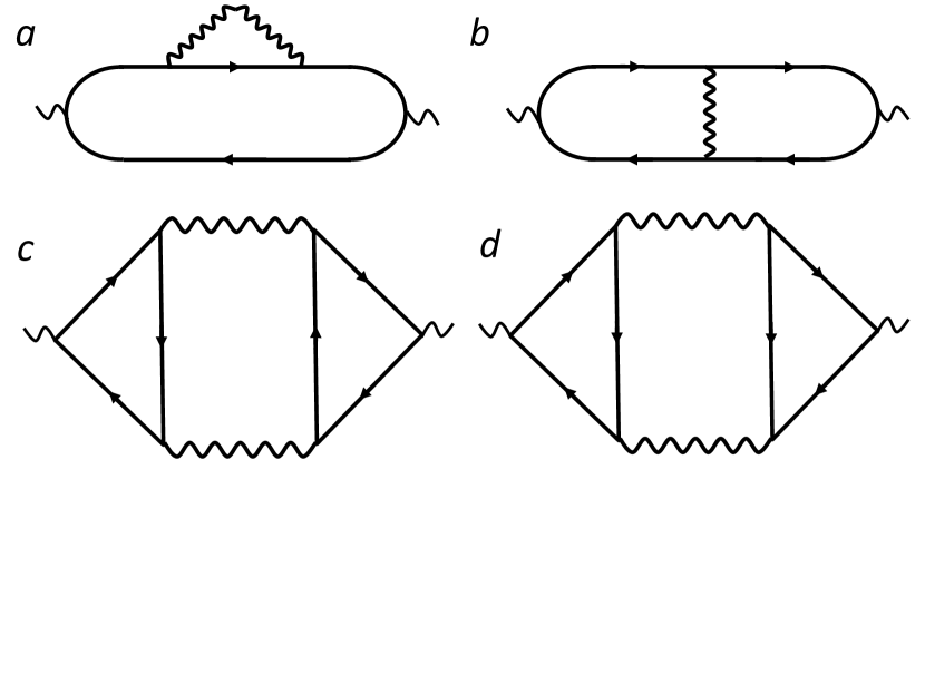
Figure 1: Maki-Thompson (a-b) and Aslamazov-Larkin (c-d) diagrams for the conductivity. The mirror image of diagram a is not shown. This solid lines denote bare Green’s functions.

The fully renormalized current-current correlator is shown in Fig. 2. It is expressed in terms of fully dressed fermionic Green’s functions and a fully dressed four-leg vertex. At small ${\bar{g}}$ and away from the critical point (but still such that $M\ll k_{F}$), the dimensionless coupling $\lambda$ is small. Then the lowest-order approximation in the fermion-boson coupling is sufficient and we go back to diagrams a-b in Fig. 1, where the solid lines are the propagators of free fermions. Evaluating these diagrams we obtain the known FL resultGurzhi (1959)

$$\sigma^{\prime}(\Omega)=\frac{\Omega_{p}^{2}}{4\pi}\frac{\gamma_{\text{tr}}(\Omega)}{\Omega^{2}},$$ (10)

where the transport scattering rate $\gamma_{\text{tr}}(\Omega)\sim(M/k_{F})^{2}\Sigma^{\prime\prime}(\Omega)$ and $\Sigma^{\prime\prime}(\Omega)\sim\lambda\Omega^{2}/\omega_{\text{FL}}\propto\Omega^{2}/M^{4}$ is the single-particle scattering rate. The smallness of $\gamma_{\text{tr}}$ compared to $\Sigma^{\prime\prime}$ reflects the fact that small-angle scattering is inefficient for momentum relaxation. Mathematically, the factor of $(M/k_{F})^{2}$ in $\gamma_{\text{tr}}$ appears because the two Maki-Thompson diagrams partially compensate each other. Substituting $\gamma_{\text{tr}}$ into Eq. (10), we find that the conductivity does not depend on frequency and scales with $M$ as

$$\sigma^{\prime}(\Omega)\propto M^{-2}.$$ (11)

This is a familiar “FL foot”: a plateau in the frequency dependence of the optical conductivity of a FL.Gurzhi (1959); Berthod et al. (2013)

A naive way to go beyond the lowest order would be to replace the bare Green’s functions in diagrams a and b in Fig. 1 by the renormalized ones, which contain the self-energies in the denominators. The real part of the self-energy would then renormalize the external frequency by a factor of $1+\lambda=1/Z$. Expanding diagram a in the imaginary part of the self-energy, we would then get instead of Eq. (11)

$$\sigma^{\prime}(\Omega)=\frac{\Omega_{p}^{2}}{4\pi}\frac{Z^{2}\gamma_{\text{tr}}(\Omega)}{\Omega^{2}}\propto\frac{Z^{2}}{M^{2}}.\,$$ (12)

If this result could be extended to a strong-coupling limit, where $Z\propto M^{2}$, we would arrive at the conductivity that is independent of $M$ in the limit of $M\to 0$. Since $M$ drops out, we would then conclude that $\sigma^{\prime}(\Omega)$ remains to be constant even right at the QCP, where $M=0$. However, it is obvious that the method described in the preceding paragraph is not consistent even in the weak-coupling limit, where $\lambda\ll 1$ and $Z\approx 1$. Indeed, recalling that $\Sigma^{\prime\prime}\propto\bar{g}$ and $Z=1+{\cal O}(\bar{g})$, we see that dependence of $\sigma^{\prime}(\Omega)$ in Eq. (12) on the coupling constant is

$$\sigma^{\prime}(\Omega)\propto\frac{\bar{g}}{[1+{\cal O}(\bar{g})]^{2}}\sim\bar{g}+{\cal O}(\bar{g}^{2})+\dots$$ (13)

Taking into account the effect of mass renormalization (the denominator in the equation above) amounts to finding a second-order correction to the conductivity in the coupling constant. This means that all second-order vertex corrections also need to be collected, but we accounted only for those which are obtained by inserting self-energy corrections into diagram b in Fig. 1.

Collecting corrections to the current vertex is simplified in our case of a long-range interaction, because the current vertex $\bar{\bf\Gamma}$ for an incoming fermion with momentum ${\bf k}$ is related to the density vertex, $\Gamma$, simply by $\bm{\bar{\Gamma}}={\bf v}_{{\bf k}}\Gamma$, up to small corrections (here, ${\bf v}_{\bf k}=\partial_{\bf k}\varepsilon_{\bf k}$). If the momentum carried by the wavy line in diagram d in Fig. 2 is ${\bf q}$, then the left current vertex in this diagram is replaced by ${\bf v}_{\bf k}\Gamma$ and the right one by ${\bf v}_{{\bf k}+{\bf q}}\Gamma$ with $k=k_{F}$. On other hand, the current vertices in diagram b give ${\bf v}_{\bf k}^{2}\Gamma^{2}$. The combination ${\bf v}_{\bf k}^{2}-{\bf v}_{{\bf k}}\cdot{\bf v}_{{\bf k}+{\bf q}}$ gives the transport factor, which we discussed above, and now the problem reduces to finding the renormalized charge vertex $\Gamma$.

The strength of the renormalization of $\Gamma$ depends on the ratio of the external momentum and frequency. We are interested in the regime where the external momentum is zero, while the external frequency ($\Omega$) is finite. [The opposite limit is discussed in Appendix A.] In this regime, the density vertex satisfies the Ward identity following from the particle number conservation: $\Gamma(\Omega)=1+\left[\Sigma(\Omega+\omega)-\Sigma(\omega)\right]/\omega$. Using $\Sigma(\omega)=\lambda\omega$, we immediately obtain $\Gamma=1+\lambda=1/Z$.

Nevertheless, inserting vertex corrections into the formula for conductivity is still a tricky issue because diagram b in Fig. 1, which we already included into Eq. (10), is also a vertex correction. This contribution and the ones that renormalize the vertex in accord with the Ward identity can be separated if one assumes that they come from different energy scales. The idea of energy scale separation in a FL (which is similar to the underlying idea of renormalization group) was put forward by Eliashberg in the context of dc conductivity Eliashberg (1962) and has been used to calculate various correlation functions of both clean Ipatova and Eliashberg (1962); Dzyaloshinskii and Larkin (1972); Shekhter et al. (2005); Chubukov and Wölfle (2014) and dirty Finkel’stein (1983); *finkelshtein:2010 FLs. In real-time formulation, this method amounts to representing a diagram for any given correlation function by a sequence of irreducible vertices separated by pairs of low-energy retarded (R) and advanced (A) Green’s functions given by Eq. (8) (“RA sections”).Finkel’stein (1983); *finkelshtein:2010 Because the method neglects diagrams with crossed irreducible vertices, it is equivalent to a kinetic equation for a FL, which takes into account the residual interaction between quasiparticles via an appropriate collision integral.Eliashberg (1962)

Any system that exhibits a FL behavior does so only at energies below certain scale which, in general, is smaller than the Fermi energy and is determined by the dynamics of the effective interaction. In our case, such “high-energy” scale is $\omega_{\text{FL}}$ given by Eq. (7). The second, “low-energy” scale is determined by energies which the system is probed at. In our case, the external frequency ($\Omega$) plays the role of such a scale.

As long as $M\neq 0$, $\omega_{\text{FL}}$ is finite, and we can choose $\Omega$ to be smaller than $\omega_{\text{FL}}$. In this situation, one can evaluate the diagrams for the conductivity by using the separation-of-scales method. Namely, one selects a cross-section containing a pair of low-energy Green’s functions [Eq. (8)] in a diagram of arbitrary order, as shown in Fig. 2c. All other elements of the diagram to the left and right of this cross-section are combined into two renormalized side vertices. Next, one selects a cross-section composed of four low-energy Green’s function intersected by a wavy line and again lumps the rest of the diagram into the left and right vertices, as shown in Fig. 2d. Then one expands the low-energy Green’s functions in diagram c to first order in $\Sigma^{\prime\prime}$ and neglects $\Sigma^{\prime\prime}$ in the Green’s functions forming the central part of diagram b. As a result, one gets diagrams of the same structure of as in Fig. 1 a and b, but with renormalized side vertices. Eliashberg (1962) The sum of the central parts of diagrams c and d in Fig. 2 yields Eq. (10), while the renormalized side vertices give two factors of $\Gamma$. The full answer then becomes

$$\sigma^{\prime}(\Omega)=\frac{\Omega_{p}^{2}}{4\pi}\frac{Z^{2}\Gamma^{2}\gamma_{\text{tr}}(\Omega)}{\Omega^{2}}\propto\frac{Z^{2}\Gamma^{2}}{M^{2}}=\frac{1}{M^{2}}.$$ (14)

In the last equation we used $\Gamma=1/Z$. This is the same result as obtained in the weak-coupling limit [Eq. (11)]: the conductivity tends to a finite value proportional to $1/M^{2}$ at low frequencies. At $M\to 0$, $\sigma^{\prime}(\Omega)$ formally diverges, but near a critical point FL regime extends only up to $\Omega\sim\omega_{\text{FL}}\propto M^{3}$. At higher frequencies, one can use standard scaling arguments and replace $M$ by $\Omega^{1/3}$. This yields $\sigma^{\prime}(\Omega)\propto 1/\Omega^{2/3}$, in agreement with the results obtained perturbatively Kim et al. (1994) and via dimensional regularization.Eberlein et al. (2016)

Note that if we were interested in a correlation function taken in the opposite limit, when $\Omega/v_{F}$ is less than the external momentum $Q$, the ladder series must have been continued by selecting more low-energy cross-sections, separated by irreducible vertices, as shown in diagrams e and f in Fig. 2. An appropriate irreducible vertex for this case would be the FL vertex $\Gamma^{\omega}$, which is related to the Landau interaction function.A. A. Abrikosov, L. P. Gorkov, and I. E. Dzyaloshinski (1963) The resummation of the geometric series in $\Gamma^{\omega}$ for, e.g., the spin susceptibility $\chi_{s}$, is necessary to reproduce the denominator in the FL result for $\chi_{s}$ in the limit of $\Omega=0$ and $Q\to 0$: $\chi_{s}=N_{F}^{*}/(1+F^{a}_{0})$, where $N_{F}^{*}$ is the renormalized density of states.Chubukov and Wölfle (2014) However, the conductivity is obtained at finite $\Omega$ and $Q=0$. In this case diagrams e, f, and similar diagrams of higher orders vanish. To see this, we label the incoming and outgoing states of the irreducible vertex (hatched box) as shown in diagram f. Since the irreducible vertex is as a high-energy object of the theory, one can safely neglect its dependence on low-energy variables, i.e., $\varepsilon_{\bf p}$, $\omega_{m}$, etc., and consider it to be a function only of the angle between ${\bf p}$ and ${\bf p}^{\prime}$. Then the integral over $\omega_{m}^{\prime}$ of the two Green’s functions to the right of the hatched box vanishes because the poles of the integrand are located in the same half-plane. We thus conclude that diagrams c and d indeed give the full result for the conductivity, provided that $\Omega/Z\gg\gamma_{\text{tr}}$.

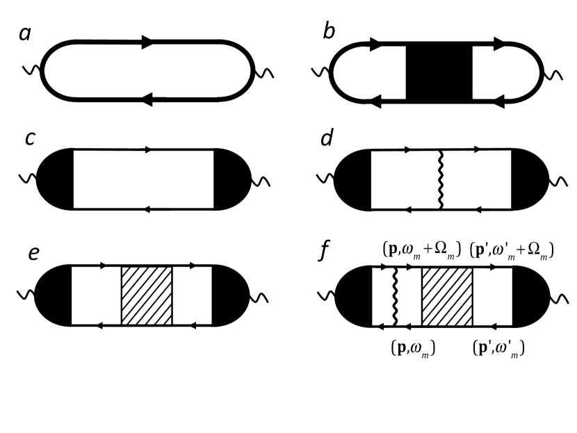
Figure 2: Separation of energy scales for the conductivity. The sum of diagrams a and b represent an exact current-current correlation function. Exact Green’s functions are denoted by thick lines. Diagram c consists of two low-energy Green’s functions given by Eq. (8) (thin lines) and current vertices, which include all high-energy renormalizations. Diagram d provides a vertex (transport) correction to diagram c. Diagrams e and f vanish for zero external momentum and finite frequency, which is the case for the conductivity.

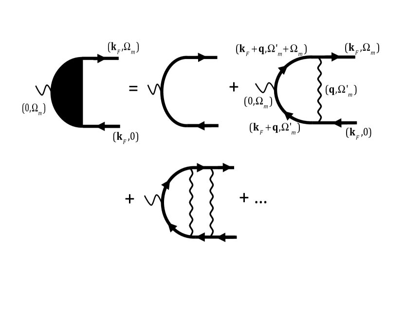
Figure 3: Vertex renormalization for a nematic QCP. Thick solid lines denote exact Green’s functions. The wavy line is the susceptibility from Eq. (4).

The issue that we address in this paper is whether it is indeed possible to separate two types of contributions to the optical conductivity: the one which determines the transport scattering rate $\gamma_{\text{tr}}$ and the one which accounts for renormalization of the current vertices. We argue that this is a non-trivial issue even in the FL regime, where we do have two different scales: $\Omega$ and $\omega_{\text{FL}}$. We show that the contributions from diagrams a and b in Fig. 1, which add up to $\gamma_{\text{tr}}$, come from internal frequencies of order $\Omega$, and this holds regardless of whether one integrates first over the internal frequency or over the fermionic dispersion $\varepsilon_{\bf k}$. The issue of vertex renormalization is more subtle. The renormalized current vertex (which, we remind, in our case is the same as the density vertex multiplied by the Fermi velocity) is obtained by summing up the ladder series shown in Fig. 3. Non-ladder diagrams are smaller at each given other. The building block ($B$) of the ladder series is the convolution of two fermionic propagators and one bosonic propagator; symbolically, $B=\int GG\chi$. The double integral over the internal frequency and fermionic dispersion is convergent, hence the result does not depend on the order of integration. Yet, characteristic internal energies, encountered when integrating in different order, differ. The fastest way to evaluate the $B$ is to integrate over $\varepsilon_{\bf k}$ first. Then the integral is determined by the poles of the fermionic propagators (see Sec. II.2.2 below). This calculation gives $B=\lambda/(1+\lambda)$. The ladder series of $B$ blocks is geometric, so the full result for the vertex is $\Gamma=1/(1-B)=1+\lambda$, in agreement with the Ward identity.

The problem with applying this approach to the conductivity is that typical internal frequencies and fermionic dispersions in $B$ are of order $\Omega$, i.e., comparable to the characteristic frequency that determine $\gamma_{\text{tr}}$. In this situation, one cannot separate a computation of vertex corrections from that of $\gamma_{\text{tr}}$. This poses a real problem because at large $\lambda$ the building block of the ladder series $B=\lambda/(1+\lambda)$ is approximately equal to unity, and the sum of such terms converges for any finite $\lambda$ only because the numerical prefactors of all terms are equal to unity as well, i.e., the series is geometric. If one cannot separate the energy scales, then each term in the ladder series gets multiplied by a factor of order $Z^{2}\gamma_{\text{tr}}/\Omega$ from the internal part of the diagram, but the numerical coefficients now do not necessary correspond to a geometric series, and the new series is not guaranteed to converge for any $\lambda<\infty$. It is also not guaranteed that the answer will contain $\Gamma^{2}$, i.e., that each side vertex in the current-current correlator gets renormalized by $1+\lambda$. The situation is even worse in the NFL regime, i.e., for $\Omega\gg\omega_{\text{FL}}$, where $\Sigma^{\prime}\sim\Sigma^{\prime\prime}\sim\omega^{1/3}_{0}\omega^{2/3}$. The energy

$$\omega_{0}=\bar{g}^{2}/v_{F}k_{F}$$ (15)

separates the perturbative regime, where $\omega\gg\omega_{0}$ and hence $|\Sigma|\ll\omega$, from the non-perturbative one, where $\omega\ll\omega_{0}$ and hence $|\Sigma|\gg\omega$. In the non-perturbative region, i.e., for external $\Omega\ll\omega_{0}$, each term in the ladder series for the vertex is a number of order one, and the series is not geometric. The solution of the integral equation for the vertex shows that ladder series is summed into Chubukov (2005) $\Gamma(\Omega)\approx(\omega_{0}/\Omega)^{1/3}\approx 1/Z(\Omega)$, in agreement with the Ward identity. However, this relation holds due to specific ratios of ${\cal O}(1)$ terms at consecutive orders. Once one combines vertex renormalization at a given order with the part of the diagram that gives $Z^{2}\gamma_{\text{tr}}/\Omega$, the ratios of terms at consecutive orders change, and there is no guarantee that the sum of ladder series will be of order $1/\Omega^{1/3}$. In addition, without a separation of scales there is no argument for why the diagrams for the current-current correlator should contain two renormalized current vertices rather than one.

We show in Sec. II.2 that the separation of scales is actually possible in the FL regime but, to apply this method in a consistent manner, one should evaluate the building block for the vertex correction in a different order: by integrating first over the fermionic frequency and then over $\varepsilon_{\bf k}$. This way, the integral over frequency comes from the branch cut in the bosonic propagator. In the Matsubara representation, this branch cut is associated with a non-analytic, $|\Omega_{m}|$ frequency dependence of the Landau damping term. In this computational scheme, typical internal $\omega$ and $\varepsilon_{\bf k}$ in $B=\int GG\chi$ are of order $\omega_{\text{FL}}$ rather than $\Omega$. Then the separation of scales is possible as long as $\Omega\ll\omega_{\text{FL}}$. As a consequence, the conductivity $\sigma^{\prime}(\Omega)$ has the form of Eq. (14). In the NFL regime, the separation of scales is not, strictly speaking, possible. Still, in Sec. II.3 we present a renormalization group-type argument which shows that the $1/M^{2}$ dependence of $\sigma^{\prime}(\Omega)$ at $M\neq 0$ translates into $\sigma^{\prime}(\Omega)\propto\Omega^{-2/3}$ in the NFL regime.

We note in passing that there exists another energy scale in the NFL regime: $\omega_{0}$ defined in Eq. (15). However, we will show below that there is no contribution to the vertex correction from this scale, no matter in what order the integrals in $B$ are evaluated.

II.2 Fermi-liquid regime
near a nematic quantum critical point

II.2.1 Central parts of diagrams for the current-current correlation function

We first analyze diagrams a and b in Fig. 1 and show that they are determined by low-energy fermions, with frequencies of order of $\Omega$, regardless of the order in which the integrals over internal frequencies and fermionic dispersions are evaluated. For definiteness and for future comparison with the calculation of the renormalized vertex, we integrate over frequency first and then over $\varepsilon_{\bf k}$.

We expect diagrams a and b to produce the FL result $\sigma^{\prime}(\Omega)\propto Z^{2}\gamma_{\text{tr}}(\Omega)/\Omega^{2}=\text{const}$. According to Eq. (9), the $\Omega$-independent $\sigma^{\prime}(\Omega)$ implies that $K^{\prime\prime}(\Omega)\propto\Omega$. The linear-in-$\Omega$ part of $K(\Omega)$ can be calculated directly on the Matsubara axis; we only have to subtract the static part of the effective interaction [Eq. (4)], because static interaction does not give rise to damping of quasiparticles and thus does not yield $K^{\prime\prime}$. The combined contribution to $K(\Omega_{m})$ from diagrams a and b reads

$$K(\Omega_{m})=e^{2}\int\frac{d^{2}q}{(2\pi)^{2}}\int\frac{d\Omega^{\prime}_{m}}{2\pi}\int\frac{d^{2}k}{(2\pi)^{2}}\int\frac{d\omega_{m}}{2\pi} \frac{\left({\bf v}_{{\bf k}}-{\bf v}_{{\bf k}+{\bf q}}\right)^{2}\chi_{\text{dyn}}(q,\Omega_{m}^{\prime})}{\left[\frac{i\omega_{m}}{Z}-\varepsilon_{\bf k}\right]\left[\frac{i\left(\omega_{m}+\Omega^{\prime}_{m}\right)}{Z}-\varepsilon_{{\bf k}+{\bf q}}\right]\left[\frac{i\Omega^{\prime}_{m}}{Z}-\varepsilon_{{\bf k}+{\bf q}}+\varepsilon_{{\bf k}}\right]\left[\frac{i(\Omega^{\prime}_{m}+\Omega_{m})}{Z}-\varepsilon_{{\bf k}+{\bf q}}+\varepsilon_{{\bf k}}\right]},$$

, (16)

where $\chi_{\text{dyn}}(q,\Omega_{m}^{\prime})=\chi(q,\Omega_{m}^{\prime})-\chi(q,0)$. The factor of $({\bf v}_{{\bf k}}-{\bf v}_{{\bf k}+{\bf q}})^{2}\propto q^{2}$ appears when we sum up diagrams a and b. Physically, it accounts for the difference between the transport and single-particle scattering rates. Since typical $q\ll k_{F}$, we approximate $\varepsilon_{{\bf k}+{\bf q}}-\varepsilon_{\bf k}$ by $v_{F}q\cos\theta$, and integrate the product of the first two factors in Eq. (16) first over $\omega_{m}$ and then over $\varepsilon_{\bf k}$. This gives

$$K(\Omega_{m})\propto Z\int dqq^{4}\int d\Omega^{\prime}_{m}\int\frac{d\theta}{2\pi}\frac{\cos\theta}{\left[\frac{i\Omega^{\prime}_{m}}{Z}-v_{F}q\cos\theta\right]^{2}\left[\frac{i(\Omega^{\prime}_{m}+\Omega_{m})}{Z}-v_{F}q\cos\theta\right]\phantom{{}^{2}}}\chi_{\text{dyn}}(q,\Omega_{m}^{\prime})$$ (17)

We assume and then verify that typical internal frequencies $\Omega_{m}^{\prime}$ are of order $\Omega_{m}$ and typical $q$ are of order $M$. For $\Omega^{\prime}_{m}\sim\Omega_{m}\ll v_{F}q\sim v_{F}M$, the angular integral in Eq. (17) is reduced to

$$\int\frac{d\theta}{2\pi}\dots=\frac{Z}{\left(\Omega_{m}v_{F}q\right)^{2}}\left(|\Omega^{\prime}_{m}|-|\Omega_{m}^{\prime}+\Omega_{m}|+\text{sgn}\Omega^{\prime}_{m}\Omega_{m}\right).$$

(18)

In the same limit, $\chi_{\text{dyn}}(q,\Omega_{m}^{\prime})\approx-\chi_{0}\gamma|\Omega_{m}^{\prime}|/q(q^{2}+M^{2})^{2}$. Substituting this into Eq. (17), we obtain

$$K(\Omega_{m}) \propto Z^{2}\int\frac{dqq}{(q^{2}+M^{2})^{2}}$$

$$\times \int\frac{d\Omega^{\prime}_{m}}{\Omega^{2}_{m}}|\Omega_{m}^{\prime}|\left(|\Omega^{\prime}_{m}|-|\Omega_{m}^{\prime}+\Omega_{m}|+\text{sgn}\Omega^{\prime}_{m}\Omega_{m}\right).$$

As expected, the integral over $q$ is determined by $q\sim M$ and gives a factor of $1/M^{2}$. The frequency integral, on the other hand, is confined to the region $0\leq|\Omega^{\prime}_{m}|\leq|\Omega_{m}|$ and gives a factor of $\Omega_{m}$. Continuing analytically from $\Omega_{m}$ to real $\Omega$, we obtain

$$K^{\prime\prime}(\Omega)\propto\frac{Z^{2}\Omega}{M^{2}}.$$ (20)

Alternatively, one can compute the integrals in Eq. (16) in a different way, but splitting ${\bf q}$ into the components tangential ($q_{||}$) and normal ($q_{\perp}$) to the FS. Integrating over $\omega_{m}$, ${\bf k}$, and $q_{||}$, we obtain

$$K(\Omega_{m}) \propto \frac{Z}{M^{2}}\int dq_{\perp}q_{\perp}$$

$$\times \int d\Omega^{{}^{\prime}}_{m}\frac{|\Omega^{{}^{\prime}}_{m}|}{\left[\frac{i\Omega^{{}^{\prime}}_{m}}{Z}-v_{F}q_{\perp}\right]^{2}\left[\frac{i(\Omega^{{}^{\prime}}_{m}+\Omega_{m})}{Z}-v_{F}q_{\perp}\right]}.$$

For a given sign of $q_{\perp}$, we now integrate over that half-plane of complex $\Omega^{{}^{\prime}}_{m}$ which does not contain poles, and choose the contour to avoid the branch cut along the imaginary axis, where $|\Omega^{{}^{\prime}}_{m}|=\pm iz$. Combining then the contributions from positive and negative $q_{\perp}$ and rescaling $q_{\perp}=x\Omega_{m}$, $z=y\Omega_{m}$, we reduce the double integral in Eq. (II.2.1) to

$$K(\Omega_{m}) \propto \frac{Z^{2}}{M^{2}}\Omega_{m}\int_{0}^{\infty}dx\int_{0}^{\infty}dy\frac{xy}{(x+y)^{3}\left[(x+y)^{2}+1\right]}$$ (22)

$$= \frac{\pi Z^{2}\Omega_{m}}{12M^{2}}.$$

Continuing analytically to real frequencies, we reproduce Eq. (20).

Equation (20) is the expected FL result: $K^{\prime\prime}(\Omega)\propto Z^{2}\gamma_{\text{tr}}/\Omega$, where $\gamma_{\text{tr}}\sim\Omega^{2}/M^{2}$, i.e., $\gamma_{\text{tr}}(\Omega)\propto M^{2}\Sigma^{\prime\prime}(\Omega)$. For our purpose, the key element of this result is that the integrals over the internal $\varepsilon_{\bf k}$ and $\Omega_{m}^{\prime}$ come from the regions confined by the external frequency $\Omega$.

We now check what are typical internal $\varepsilon_{\bf k}$ and $\Omega_{m}^{\prime}$ in the vertex correction diagrams.

II.2.2 Vertex renormalizaton

The diagrammatic series for the charge vertex $\Gamma$ at zero external momentum and finite external frequency $\Omega_{m}$ is shown in Fig. 3. The fermionic Green’s functions in this series are the full ones: $G({\bf k},\omega_{m})=\left[i\omega_{m}+\Sigma(\omega_{m})-\varepsilon_{{\bf k}}\right]^{-1}$. We remind that this form reduces to

$$G({\bf k},\omega_{m})=\left[i\omega_{m}(1+\lambda)-\varepsilon_{{\bf k}}\right]^{-1}$$ (23)

for $\omega_{m}\ll\omega_{\text{FL}}$. As in the previous section, we assume that $T=0$, in which case bosonic and fermionic Matsubara frequencies are continuous variables. For simplicity, we set the frequency of an incoming fermion to be zero (then the frequency of an outgoing fermion is $\Omega_{m}$), and set the fermionic momentum (which is the same for incoming and outgoing fermions) to be ${\bf k}_{F}\equiv k_{F}{\bf k}/k$. The series reads

$$\Gamma=1+\Gamma_{1}+...,$$ (24)

where

$$\Gamma_{1} = g^{2}\int\frac{d\Omega^{\prime}_{m}}{2\pi}\int\frac{d^{2}q}{(2\pi)^{2}}G({\bf k}^{\prime},\Omega^{\prime}_{m})G({\bf k}^{\prime},\Omega^{\prime}_{m}+\Omega_{m})$$ (25)

$$\times\chi(q,\Omega^{\prime}_{m})$$

and ${\bf k}^{\prime}={\bf k}_{F}+{\bf q}$. We remind that $g^{2}$ is related to ${\bar{g}}$, which we used earlier, by ${\bar{g}}=g^{2}\chi_{0}$. As before, the bosonic momentum ${\bf q}$ can be decomposed into the components perpendicular and tangential to the FS, $q_{\perp}$ and $q_{||}$, correspondingly. With this decomposition, the fermionic dispersion in the Green’s functions entering Eq. (25) can be approximated as $\varepsilon_{{\bf k}^{\prime}}=v_{F}q_{\perp}$.

We assume and then verify that typical $q_{\perp}$ in the integral in Eq. (25) are much smaller than typical $q_{||}$. Using this assumption, we neglect $q_{\perp}$ in $\chi(q,\Omega_{m}^{\prime})$. Integration over $q_{||}$ is then elementary and gives an effective local susceptibility

$$\chi_{L}(\Omega^{\prime}_{m})=\int\frac{dq_{||}}{2\pi}\chi(q_{||},\Omega^{\prime}_{m})=\frac{\chi_{0}}{2M}f_{L}\left(\frac{|\Omega^{\prime}_{m}|}{\omega_{\text{FL}}}\right),$$ (26)

where $f_{L}(x\ll 1)=1+{\cal O}(x)$ and $f_{L}(x\gg 1)\propto x^{-1/3}$.

The double integral over $\Omega^{\prime}_{m}$ and $\varepsilon_{{\bf k}^{\prime}}=v_{F}q_{\perp}$ is convergent in the ultraviolet, and thus the order of integration should not matter. At the same time, the structure of the integrand is not symmetric with respect to $\Omega^{\prime}_{m}$ and $\varepsilon_{{\bf k}^{\prime}}$, and characteristic values of $\Omega^{\prime}_{m}$ and $\varepsilon_{{\bf k}^{\prime}}$, which contribute mostly to the integral, are not necessary the same.

Because the integral over $\Omega_{m}^{\prime}$ formally extends into the regions where the low-energy form of the Green’s function, Eq. (23), is not valid, it is tempting to integrate in Eq. (25) over $\varepsilon_{{\bf k}^{\prime}}$ first. The integral over $\varepsilon_{{\bf k}^{\prime}}$ is non-zero only if the poles of Green’s functions are located in the opposite half-planes of $\varepsilon_{{\bf k}^{\prime}}$, which implies that the internal frequencies are confined to the interval $-\Omega_{m}\leq\Omega^{\prime}_{m}<0$ for $\Omega_{m}>0$ and to a similar interval for $\Omega_{m}<0$. Using this form, we obtain in the FL regime ($\Omega_{m}\ll\omega_{\text{FL}}$):

$$\Gamma_{1}=\frac{\lambda}{1+\lambda}.$$ (27)

Evaluating higher-order diagrams in the same way, we find that they form a geometric series $1+\Gamma_{1}+\Gamma_{1}^{2}+..=1/(1-\Gamma_{1})$. Then the full vertex is

$$\Gamma=\frac{1}{1-\Gamma_{1}}=\frac{1}{1-\frac{\lambda}{1+\lambda}}=1+\lambda.$$ (28)

This in agreement with the Ward identity $\Gamma(\Omega)=1+\partial\Sigma(\omega_{m})/\partial(i\omega_{m})$.

We see, however, that in this computational procedure the internal frequencies $\Omega_{m}^{\prime}$ are of the same order as the external one ($\Omega_{m}$), and typical $\varepsilon_{{\bf k}^{\prime}}$ are of order of $(1+\lambda)\Omega_{m}$. As we said in the previous section, this creates an ambiguity when the diagrammatic series for vertex renormalization are combined with the central parts of diagrams c and d in Fig. 2, as these parts and vertex corrections come from the same energy interval.

We now show that if the order of integrations over $\Omega^{\prime}_{m}$ and $\varepsilon_{{\bf k}^{\prime}}$ in Eq. (25) is interchanged, the result remains the same, but typical $\Omega^{\prime}_{m}$ are now of order of $\omega_{{\rm FL}}$ rather than of $\Omega_{m}$. For $\Omega_{m}\ll\omega_{{\rm FL}}$, this provides a justification for the separation of scales, which is required for the validity of Eq. (14).

Integration in Eq. (25) over frequency is rather complicated due to the presence of self-energies in the Green’s functions. These self-energies cannot be replaced by either FL or NFL forms because, as will see, at least part of the result comes from the crossover region between the two forms. The integrand in Eq. (25), viewed as a function of $\Omega^{\prime}_{m}$, has poles from the Green’s functions and branch cuts from both the bosonic propagator and self-energy. For a given sign of $\varepsilon_{{\bf k}^{\prime}}$, the poles of the two Green’s functions are in the same half-plane of $\Omega^{\prime}_{m}$, even if external $\Omega_{m}$ is non-zero. The branch cuts emerge because $\chi(q,\Omega^{\prime}_{m})$ has a non-analytic, $|\Omega^{\prime}_{m}|$ dependence on the frequency. In $\chi(q,\Omega^{\prime}_{m})$, viewed as a function of complex $\Omega^{\prime}_{m}$, the branch cut is along the imaginary frequency axis (for $\omega_{m}=iz+\delta$, $|\omega_{m}|=iz\text{sgn}\delta$), and it runs along both positive and negative parts of the imaginary axis. A convenient way to compute $\Gamma_{1}$ is then to split the integral over $\varepsilon_{{\bf k}^{\prime}}$ into two integrals over positive and negative $\varepsilon_{{\bf k}^{\prime}}$. For each sign of $\varepsilon_{{\bf k}^{\prime}}$, we close the integration contour in that half-plane which does not contain poles and choose the branch cut to be in the same half-plane. In this way, only the integral along the branch cut contributes to the final result.

A closer look at the integral over the branch cut shows that it is controlled by energy scales that are much larger than $\Omega_{m}$ and therefore can be evaluated at $\Omega_{m}=0$. One such scale is $\omega_{{\rm FL}}$, defined in Eq. (7), and another one is $\omega_{0}$, defined in Eq. (15). Note that $\omega_{0}\sim\omega_{{\rm FL}}\lambda^{3}\gg\omega_{\text{FL}}$. The contributions from $\omega_{m}\sim\omega_{{\rm FL}}$ and from $\omega_{m}\sim\omega_{0}$ can be computed independently from each other and yield $\Gamma_{1}=\Gamma_{1,\omega_{0}}+\Gamma_{1,\omega_{\text{FL}}}$. After some involved algebra, we find

$$\Gamma_{1,\omega_{0}}=\frac{2}{3\pi}\int_{0}^{\infty}\frac{dx}{x^{2/3}+x^{4/3}+\sqrt{3}x}=\frac{2}{3},$$

$$\Gamma_{1,\omega_{{\rm FL}}}=C-\frac{1}{\lambda+1},$$ (29)

where $C$ is independent of $\lambda$. This term was obtained numerically because an analytic form of $\Sigma(\omega_{m})$ at finite $M$ and arbitrary $\omega_{m}$ is not known. However, numerical evaluation of $C$ is straightforward, and we found that $C=1/3$ to high numerical accuracy. The two contributions to $\Gamma_{1}$ then add up to

$$\Gamma_{1}=\frac{\lambda}{1+\lambda}.$$ (30)

This is the same result as before, but now $\Gamma_{1}$ comes from energies which are much higher than $\Omega_{m}$.

Taken at face value, Eq. (29) implies that $\Gamma_{1}$ comes partially from $\Omega^{\prime}_{m}\sim\omega_{{\rm FL}}$ and partially from $\Omega^{\prime}_{m}\sim\omega_{0}$. On a more closer look, however, we found that there is a peculiar cancellation between $\Gamma_{1,\omega_{0}}$ and a portion of $\Gamma_{1,\omega_{{\rm FL}}}$. Namely, $\Gamma_{1,\omega_{{\rm FL}}}$ can be split into two contributions – one is obtained by approximating the fermionic self-energy by $\Sigma(\Omega^{\prime}_{m})=i\lambda\Omega^{\prime}_{m}$, and another is obtained by subtracting $i\lambda\Omega^{\prime}_{m}$ from $\Sigma(\Omega^{\prime}_{m})$. In both terms, typical internal frequencies are of order $\omega_{\text{FL}}$, and the two expressions are of the same order because at $\Omega^{\prime}_{m}\sim\omega_{\text{FL}}$, $\Sigma(\Omega^{\prime}_{m})$ differs from $i\lambda\Omega^{\prime}_{m}$ by terms of comparable magnitude. Evaluating the two parts of $\Gamma_{1,\omega_{0}}$ separately, we find that the first one gives $\frac{\lambda}{1+\lambda}$, while the second gives $-\frac{2}{3}$ and cancels out $\Gamma_{1,\omega_{0}}$. This indicates that the contribution to $\Gamma_{1}$ can be viewed as coming entirely from the range $\Omega^{\prime}_{m}\sim\omega_{{\rm FL}}$. Still, what is essential for our purposes is that characteristic $\Omega^{\prime}_{m}\sim\omega_{{\rm FL}}$ in the vertex correction diagrams is larger than characteristic $\Omega^{\prime}_{m}\sim\Omega_{m}$ in the internal parts of diagrams c and d in Fig. 2. We re-iterate that this separation of scales only holds if we integrate over fermionic frequency first and then over fermionic dispersion.

The difference between characteristic $\Omega^{\prime}_{m}$ and $\varepsilon_{\bf k}$ in the vertex correction diagram in the FL regime also holds if one calculates vertex corrections in the opposite, static limit, when the external momentum $Q$ is non-zero, while the external frequency $\Omega_{m}$ is zero. We discuss this issue in Appendix A.

II.2.3 Final result for the conductivity in the Fermi-liquid regime

The separation between characteristic energies in those parts of the current-current correlator, which determine $\gamma_{\text{tr}}$, and those, which determine vertex corrections, justifies the decomposition of the full correlator, given by diagrams a and b in Fig. 2, into the sum of diagrams c and d. The internal parts and side vertices in diagrams c and d are computed independently of each other. The final result for the conductivity in the FL regime is then rigorously established to be

$$\sigma^{\prime}(\Omega)\propto\frac{(\Gamma Z)^{2}}{M^{2}}\sim\frac{1}{M^{2}}\sim\frac{1}{\omega^{2/3}_{\text{FL}}}.$$ (31)

II.3 Nematic quantum critical point

At the QCP, $\omega_{{\rm FL}}=0$, and the separation of energy scales does not hold. Still, Eq. (31) does allow one to determine $\sigma(\Omega)$ even at the QCP under an additional assumption that $\omega_{{\rm FL}}$ is the only energy scale near a nematic QCP. This assumption is consistent with perturbative calculations. Combining this assumption with Eq. (31), we conjecture that the conductivity behaves as $\sigma^{\prime}(\Omega)\propto\omega^{-2/3}_{FL}f(\Omega/\omega_{{\rm FL}})$, with $f(0)=1$. Another constraint on function $f(x)$ is imposed by the requirement that $\omega_{\text{FL}}$ should not enter the result in the quantum-critical regime, where $\Omega\gg\omega_{\text{FL}}$. This is only possible if $f(x)\propto x^{-2/3}$ for $x\to\infty$. This in turn implies that $\sigma^{\prime}(\Omega)\propto\Omega^{-2/3}$ at the QCP, in agreement with Refs. Kim et al., 1994 and Eberlein et al., 2016.

The scaling argument can also be cast into the renormalization-group language, if we formally introduce a lower cutoff in the bosonic momentum along the FS at some $q_{1}\sim(\gamma\omega_{1})^{1/3}$, where $\omega_{1}$ is larger than $\Omega$ but smaller than $\omega_{0}$. This cutoff effectively re-introduces the mass into the bosonic propagator at the QCP. As the result, the fermionic self-energy $\Sigma(\omega)$ and local susceptibility $\chi_{L}(\Omega)$ become scaling functions of $\omega/\omega_{1}$ and $\Omega/\omega_{1}$, and display a FL behavior at $\omega,\Omega\ll\omega_{1}$. Accordingly, the conductivity scales as $\sigma^{\prime}(\Omega)\propto\omega^{-2/3}_{1}$. One can then make $\omega_{1}$ progressively smaller and get progressively larger conductivity. The scaling $\sigma^{\prime}(\Omega)\propto\omega^{-2/3}_{1}$ holds as long as $\omega_{1}\gg\Omega$. At $\Omega\lesssim\omega_{1}$, scaling with $\omega_{1}$ is replaced by that with $\Omega$, which yields again $\sigma^{\prime}(\Omega)\propto\Omega^{-2/3}$.

III Spin-density-wave
quantum critical point

The correlation function of antiferromagnetic fluctuations near a SDW QCP,

$$\chi({\bf q},\Omega_{m})=\frac{\chi_{0}}{({\bf q}-{\bf q}_{\pi})^{2}+M^{2}+\gamma|\Omega_{m}|},$$ (32)

is peaked at the nesting momentum ${\bf q}_{\pi}$ which connects hot spots on the Fermi surface. For a 2D square lattice, ${\bf q}=(\pi,\pi)$ (the lattice constant is set to unity). Two out of eight hot spots are shown by red circles in Fig. 4, panels a and b. In what follows, we will consider the contributions to the optical conductivity both from “hot fermions”, located near the hot spots, and from “lukewarm fermions”,Hartnoll et al. (2011); Chubukov et al. (2014) occupying the regions between the hot spots and cold parts of the FS (the cold and lukewarm regions are depicted as blue and orange areas, correspondingly, in Fig. 4 a and b).

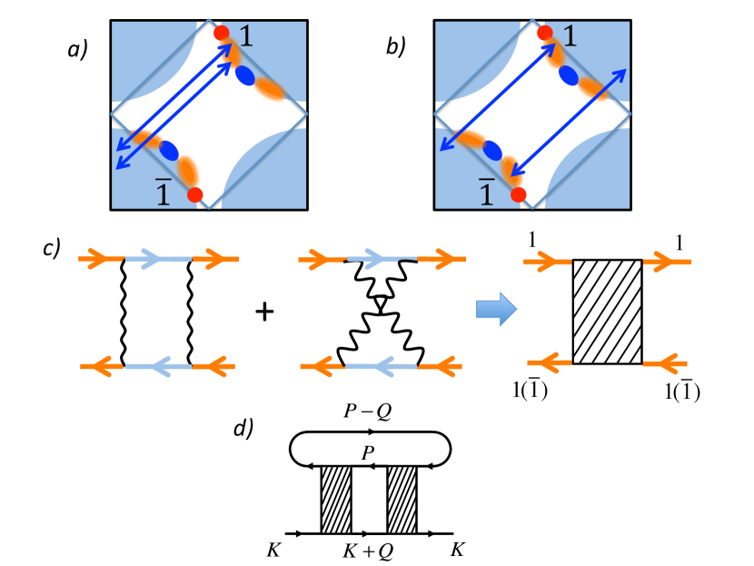
Figure 4: a and b: A Fermi surface of a 2D metal near a SDW QCP. Red circles: hot spots; blue areas: cold regions; orange areas: lukewarm regions. Arrows indicate a composite scattering process which involves lukewarm fermions either from the same (a) or diametrically opposite (b) regions. c: Composite scattering vertex. The initial states on the bottom can belong either to lukewarm regions $1$ or $\bar{1}$. d: Two-loop composite self-energy.

III.1 Conductivity of hot fermions

The main interaction mechanism for hot fermions is SDW scattering by momentum ${\bf q}_{\pi}$, mediated by the effective interaction in Eq. (32). To one-loop order, this interaction leads to a singular behavior of the self-energy at the hot spots (${\bf k}={\bf k}_{\text{hs}}$), where $\Sigma({\bf k}_{\text{hs}},\omega)\propto\omega^{1/2}$. Away from the hot spots, this singular behavior holds in a range of $|{\bf k}-{\bf k}_{\text{hs}}|$ whose width by itself scales as $\sqrt{\omega}$. This additional factor of $\sqrt{\omega}$ can be incorporated into the transport scattering rate and, beyond that, does not affect our consideration. For scattering peaked at the nesting momentum, the velocities at two hot spots connected by ${\bf q}_{\pi}$, ${\bf v}_{\bf k}$ and ${\bf v}_{{\bf k}+{\bf q}_{\pi}}$, have equal magnitudes but generally differ in direction. On one hand, this implies that the factor $({\bf v}_{\bf k}-{\bf v}_{{\bf k}+{\bf q}_{\pi}})^{2}$ in the transport scattering rate does not introduce additional smallness, i.e., $\gamma_{\text{tr}}$ and FS-averaged $\Sigma^{\prime\prime}(\omega)$ are of the same order. On the other hand, renormalizations of the current vertices at the initial and final points of a SDW scattering process (${\bf k}$ and ${\bf k}+{\bf q}_{\pi}$, correspondingly) are mixed in the perturbation theory.

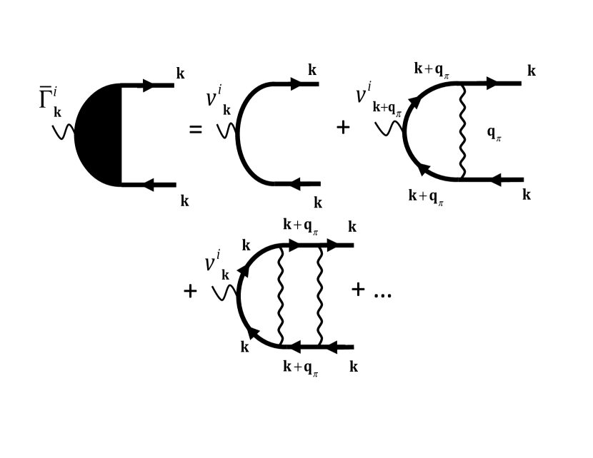
Figure 5: Diagrammatic series for the current vertex near a SDW QCP. ${\bf k}$ is chosen at a hot spot and ${\bf k}+{\bf q}_{\pi}$ is at another hot spot, connected to the first one by the nesting momentum, ${\bf q}_{\pi}=(\pi,\pi)$. The superscript $i$ denotes the $i^{\text{th}}$ Cartesian component of the corresponding vector. The series for the vertex at ${\bf k}+{\bf q}_{\pi}$ is obtained from that shown in the figure by relabeling ${\bf k}\leftrightarrow{\bf k}+{\bf q}_{\pi}$.

To get an insight into this mixing, we consider again the FL regime, where the self-energy near a hot spot is described by $\Sigma(\omega_{m})=i\lambda\omega_{m}$, and vertex renormalization is described by a geometric series of ladder diagrams. The series for the $i^{\text{th}}$ Cartesian component of $\bm{\bar{\Gamma}}_{{\bf k}}$ is shown in Fig. 5; the series for $\bm{\bar{\Gamma}}_{{\bf k}+{\bf q}_{\pi}}$ is obtained by relabeling ${\bf k}\leftrightarrow{\bf k}+{\bf q}_{\pi}$. Performing the same calculations as for the nematic case, we obtain

$${\bar{\Gamma}}^{i}_{\bf k}=\frac{v^{i}_{\bf k}+\frac{\lambda}{1+\lambda}v^{i}_{{\bf k}+{\bf q}_{\pi}}}{1-\left(\frac{\lambda}{1+\lambda}\right)^{2}},$$

$${\bar{\Gamma}}^{i}_{{\bf k}+{\bf q}_{\pi}}=\frac{v^{i}_{{\bf k}+{\bf q}_{\pi}}+\frac{\lambda}{1+\lambda}v^{i}_{{\bf k}}}{1-\left(\frac{\lambda}{1+\lambda}\right)^{2}}.$$ (33)

Each of the vertices in Eq. (33) diverges at criticality, where $\lambda\to\infty$. However, one can readily verify that for the SDW case the sum of diagrams c and d in Fig. 2 is equal to diagram c with side vertices ${\bar{\Gamma}}^{i}_{\bf k}-{\bar{\Gamma}}^{i}_{{\bf k}+{\bf q}_{\pi}}$. From Eq. (33) we see that this difference is finite at $\lambda\to\infty$:

$${\bar{\Gamma}}^{i}_{\bf k}-{\bar{\Gamma}}^{i}_{{\bf k}+{\bf q}_{\pi}}=\frac{v^{i}_{\bf k}-v^{i}_{{\bf k}+{\bf q}_{\pi}}}{1+\frac{\lambda}{1+\lambda}}\approx\frac{1}{2}\left(v^{i}_{\bf k}-v^{i}_{{\bf k}+{\bf q}_{\pi}}\right).$$ (34)

Therefore the effective current vertex, which appears in the expression for the conductivity, does not undergo singular renormalization. As a result, the fermionic $Z$-factor does not cancel out from the conductivity, and we have $\sigma^{\prime}(\Omega)\propto Z^{2}\gamma_{\text{tr}}/\Omega^{2}$. [We remind that in our local theory there is a one-to-one correspondence between the $Z$-factor and the renormalized mass: $Z=m_{b}/m^{*}$. It is expected that in a more general case, when this relation does not hold, the $Z$-factor is to be replaced by $m_{b}/m^{*}$.] In the FL regime, $Z\propto M$ and $\Sigma^{\prime\prime}(\Omega)\propto\Omega^{2}/M^{3}$. The role $\gamma_{\text{tr}}$ is played by the FS average of $\Sigma^{\prime\prime}$, which differs from $\Sigma^{\prime\prime}$ by the angular width of the hot spot. This width by itself scales as $M$; thus $\gamma_{\text{tr}}\propto\Omega^{2}/M^{2}$. Collecting all the factors together, we find that $\sigma^{\prime}(\Omega)$ tends to an $M$-independent value at $\Omega\to 0$. At the QCP, $Z\propto\sqrt{\Omega}$, $\gamma_{\text{tr}}\propto\sqrt{\Omega}\times\sqrt{\Omega}=\Omega$, and $\sigma^{\prime}(\Omega)$ again remains constant at $\Omega\to 0$.

The results presented above imply that the extended Drude formula [Eq. (1)] correctly describes the hot-fermion conductivity. Higher-order self-energy and vertex corrections do contain additional factors of $\ln{\Omega}$, and a series of such terms may give rise to a singular behavior of the hot-fermion conductivity. Still, Eq. (1) is expected to be valid except, possibly, very frequencies.

III.2 Conductivity of lukewarm fermions

Previous studiesHartnoll et al. (2011); Chubukov et al. (2014); Maslov and Chubukov (2017) found that the hot-spot contribution to the conductivity is not the dominant one at low frequencies, when there is a clear distinction between hot and cold regions of the Fermi surface (at high enough frequencies, the full Fermi surface becomes “hot” Abanov et al. (2003)). The dominant contribution to the optical conductivity actually comes from lukewarm regions, located in between hot and cold regions on the Fermi surface. Fermions in the lukewarm regions (orange areas in Fig. 4, a and b) form a FL state even if the system is right at the SDW criticality. However, this is a strongly renormalized FL with a $Z$-factor which varies from zero at the hot spot to $Z\approx 1$ in the cold region. In the bulk of the lukewarm region, the $Z$-factor scales linearly with the distance along the FS measured from the nearest hot spot: $Z\sim k_{||}v_{F}/\bar{g}\ll 1$. The most relevant interaction process for lukewarm fermions is composite scattering,Hartnoll et al. (2011) which consists of two consequent events of scattering by ${\bf q}_{\pi}$. Because a lukewarm fermion is not at the hot spot, the first scattering event by ${\bf q}_{\pi}$ takes it to an off-shell state away from the FS, and the second event brings it back to near where it started. In principle, fermions of all the eight hot spots can be involved in composite scattering, but the the corresponding two-loop self-energy (Fig. 4d) is logarithmically enhanced in two cases: if the lukewarm fermions belong to same region (“forward scattering”, shown in Fig. 4a) or diametrically opposite regions (“$2k_{F}$-scattering”, shown in Fig. 4b). The corresponding scattering vertices are shown in Fig. 4c. For lukewarm fermions at distances $p_{||}$ and $k_{||}$ from the corresponding hot spot(s), the composite vertex with momentum transfer $q$ and frequency transfer $\omega$ is of order $\Gamma_{\text{c}}\sim(\bar{g}/k_{||}p_{||})\ln\left(\Lambda/\max\{\omega,v_{F}q\}\right)$.

The most singular contribution to the optical conductivity occurs at two-loop order in composite scattering. Depending on the energy the system of lukewarm fermions is probed at, it behaves either as a 1D or 2D system. For the optical conductivity, the energy scale separating the two regimes is $\Omega_{12}\sim\bar{g}^{2}/E_{F}$.

For $\Omega>\Omega_{12}$, the energy cost of displacing a lukewarm fermion tangentially to the FS is small, which means that the curvature of the Fermi surface can be neglected, and we are in the 1D regime. The corresponding self-energy exhibits a linear scaling with frequency $\Sigma^{\prime\prime}\propto\Omega$, which is characteristic for 1D.Maslov (2004) The main contribution to $\sigma^{\prime}(\Omega)$ in this regime comes from the boundary between the lukewarm and cold regions of the FS, where $Z\sim 1$ (Refs. Hartnoll et al., 2011; Chubukov et al., 2014; Maslov and Chubukov, 2017). In this case, Eq. (2) with $\gamma_{\text{tr}}\sim\Sigma^{\prime\prime}\propto\Omega$ predicts that

$$\sigma^{\prime}(\Omega)\propto 1/\Omega.$$ (35)

For $\Omega<\Omega_{12}$, the FS curvature cannot be neglected, and we are in the 2D regime. The main contribution to $\sigma^{\prime}(\Omega)$ comes from the region of $k_{||}\propto\Omega^{1/3}$ (Refs. Hartnoll et al., 2011; Chubukov et al., 2014; Maslov and Chubukov, 2017), where the $Z$-factor is small: $Z\propto k_{||}\propto\Omega^{1/3}\ll 1$. Therefore, the question whether renormalization of the $Z$-factor affects $\sigma^{\prime}(\Omega)$ is again relevant.

The two-loop self-energy in the 2D regime is of the FL type $\Sigma^{\prime\prime}(\Omega)\propto(\Omega^{2}/k_{||}^{4})\ln^{3}(\Omega_{12}/\Omega)$ (the factor of $1/k_{||}^{4}$ comes from the product of two composite vertices in Fig. 4d). The corresponding Maki-Thompson diagrams for the conductivity are shown in Fig. 6. (As before, we neglect the Aslamazov-Larkin diagrams which would only modify the result by a factor of order one because our system is on a lattice.) The current vertices in these diagrams are formed by one-loop ${\bf q}_{\pi}$ scattering, which is still the main process leading to renormalization of the $Z$-factor. However, although the composite vertices (hatched blocks) are constructed from two ${\bf q}_{\pi}$ scattering processes, they effectively scatter fermions only by small angles. In Fig. 6, we depicted a particular $2k_{F}$ composite scattering processes, in which the two incoming fermions belong to diametrically opposite lukewarm regions ($1$ and $\bar{1}$). The current vertices in both diagrams a and b belong to the same lukewarm region ($1$). In diagram a, the left and right current vertices are evaluated at the same momentum. In diagram b, the momenta in the left and right current vertices differ by a small momentum transfer through the composite vertex. In this sense, the situation is now similar to the nematic QCP but partial cancellation between diagrams a and b affects only the logarithmic factors in the self-energy. Chubukov et al. (2014); Maslov and Chubukov (2017) As a result, $\gamma_{\text{tr}}(\Omega)\sim\Sigma^{\prime\prime}(\Omega)/\ln^{3}(\Omega_{12}/\Omega)\propto\Omega^{2}/k_{||}^{4}$. If renormalization of the current vertices is neglected, the conductivity is obtained from Eq. (2) by replacing $Z$ and $\gamma_{\text{tr}}(\Omega)$ by their values at given $k_{||}$ and averaging over $k_{||}$. The lower limit of the momentum integration is $k_{||}\sim\Omega^{1/3}$, while the upper limit can be set to infinity due to a rapid convergence of the integral. Then we would obtain $\sigma^{\prime}(\Omega)\propto\int^{\infty}_{\Omega^{1/3}}dk_{||}Z^{2}\gamma_{\text{tr}}(\Omega)/\Omega^{2}\propto 1/\Omega^{1/3}$. This is the result reported in Refs. Hartnoll et al., 2011; Chubukov et al., 2014; Maslov and Chubukov, 2017.

We now follow the analysis of a nematic QCP and take renormalization of the current vertices into account. Each of the current vertices diverges at criticality as specified by Eq. (33), i.e., $\bar{\Gamma}^{i}_{{\bf k}}\propto\lambda\sim 1/Z\propto 1/k_{||}$. Consequently, the result for the conductivity is changed to

$$\sigma^{\prime}(\Omega)\propto\frac{1}{\Omega^{2}}\int^{\infty}_{\Omega^{1/3}}dk_{||}\left(\bar{\Gamma}^{i}_{{\bf k}}Z\right)^{2}\gamma_{\text{tr}}(\Omega)\propto\frac{1}{\Omega}.$$ (36)

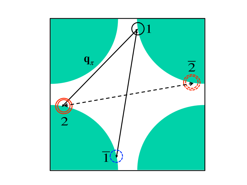
Figure 6: Maki-Thompson diagrams for the conductivity of lukewarm fermions (the mirror image of diagram b is not shown.) Hatched boxes represent composite scattering vertices shown in Fig. 4c. Current vertices are renormalized by ${\bf q}_{\pi}$ scattering as shown in Fig. 5. Labels $1$ and $\bar{1}$ correspond to the lukewarm regions in Fig. 4, a and b.

The key part of the this result is a cancellation between the $Z$-factor and $\bar{\Gamma}^{i}_{{\bf k}}$ which, as for the nematic case, leads to a breakdown of the extended Drude formula [Eq. (1)]. As the consequence, the $1/\Omega$ scaling of $\sigma^{\prime}(\Omega)$ extends from the 1D regime [Eq. (35)] down to the lowest frequencies.

Comparing the hot-spot and lukewarm contributions to the conductivity, we see that the latter is much larger, both in the 2D and 1D regimes. Eventually, the full Fermi surface becomes hot, Abanov et al. (2003) but this happens only at high enough frequencies. Therefore, $\sigma^{\prime}(\Omega)$ at a SDW QCP scales as $1/\Omega$. We note in passing that such scaling is consistent with the marginal-FL phenomenology Varma et al. (1989); *varma:2002 and observed scaling of $\sigma^{\prime}(\Omega)$ in the high-$T_{c}$ cuprates. Basov et al. (1996); *puchkov:1996; *norman:2006

IV Conclusions

The question of how renormalization of the electron effective mass affects the conductivity has a long history, which goes back to the seminal papers by Langer on the residual resistivity of a FLLanger (1960) and by Langreth and Kadanoff on polaronic transport. Langreth and Kadanoff (1964) Nowadays, this question has acquired particular importance in the context of correlated electron systems near quantum phase transitions, where the renormalized mass is expected to depend on the temperature or frequency, thus potentially affecting the corresponding dependences of the conductivity. A phenomenological way to account for these extra dependences is via the “extended Drude formula”Basov et al. (2011) of the type given by Eq. (1), which contains the renormalized (and thus $\Omega$- and $T$-dependent) mass.

In this paper, we studied the optical conductivity within two specific models of quantum criticality of the nematic and spin-density-wave types. In both cases, the critical theory is local, and the effective mass is same as the inverse quasiparticle $Z$ factor. We found that in the nematic case the effect of mass renormalization is canceled by renormalization of current vertices. This is consistent with earlier works. Kim et al. (1994); Eberlein et al. (2016) The resultant conductivity, $\sigma^{\prime}(\Omega)\propto\Omega^{-2/3}$ is consistent with the Drude formula which contains a bare rather than renormalized mass. The spin-density-wave case happens to be more subtle. There are two contributions to the conductivity from two qualitatively different regions of the Fermi surface: hot spots, connected by the nesting vector, and lukewarm regions, occupying the space in between hot and cold parts of the Fermi surface. We found no cancelation between the mass and current vertex for the hot-fermion contribution. In this situation, the correct result for the conductivity is reproduced by the Drude formula with the renormalized mass. On the other hand, this cancellation does occur for the lukewarm-fermion contribution, which is the dominant one. The resultant conductivity at a SDW QCP is then $\sigma^{\prime}(\Omega)\propto 1/\Omega$.

In view of these results, we believe that the short answer to the question ”bare vs renormalized mass” is ”it depends on the situation considered”. For example, the dc conductivity of electrons coupled to optical phonons contains the bare mass in the adiabatic regime, when the electron energy is higher than the phonon one, and the renormalized mass in the anti-adiabatic regime,Langreth and Kadanoff (1964) when the electron energy is lower than the phonon one. The three cases that we considered here provide three more examples which demonstrate the absence of the universal answer to the question about the type of the effective mass entering the conductivity. Indeed, whether the conductivity of a quantum-critical system contains the bare or renormalized mass turns out to depend not only on the type of criticality ($q=0$ vs finite $q$ QCP), but also on particular scattering processes considered for a given type. Overall, one implication of our study is that the extended Drude formula need to be treated with a great caution.

One more reason for exercising caution is that Eq. (1) is not the only form of the extended Drude formula. Another version of this formula can be derived from the kinetic equation for a FL:P. Nozières and D. Pines (1966); Lifshitz and Pitaevskii (1981)

$$\sigma^{\prime}(\Omega)=\frac{\Omega_{p}^{2}}{4\pi}\frac{m_{b}}{m^{*}}\frac{\tilde{\gamma}_{\text{tr}}(\Omega)}{\left(\Omega\frac{m_{b}}{m^{*}}\right)^{2}+\tilde{\gamma}^{2}_{\text{tr}}(\Omega)}.$$ (37)

In this version, the frequency in the denominator is divided by the renormalized mass, which is opposite to what Eqs. (1) says. Note, however, the transport scattering rate in Eq. (37) is introduced phenomenologically and cannot be a priori associated with the fermionic self-energy, even if a transport correction is accounted for. As pointed out in Ref. Kim et al., 1994, Eq. (37) can be made consistent with the result $\sigma^{\prime}(\Omega)\propto\Omega^{-2/3}$ for a nematic QCP by redefining the transport scattering rate as $\gamma^{*}_{\text{tr}}=\tilde{\gamma}_{\text{tr}}(m^{*}/m_{b})$ and assuming that it is $\gamma^{*}_{\text{tr}}$ rather than $\tilde{\gamma}_{\text{tr}}$ that scales as $\Omega^{4/3}$ at criticality. Such a redefinition changes Eq. (37) to $\sigma^{\prime}(\Omega)=\Omega_{p}^{2}\gamma^{*}_{\text{tr}}/\left[4\pi\left(\Omega^{2}+\gamma^{*2}_{\text{tr}}\right)\right]$ which does not contain the renormalized mass.

Appendix A Vertex corrections at finite external momentum and zero external frequency

For completeness, we analyze in this Appendix vertex renormalization in the situation when the the incoming frequency is set to zero while keeping the external momentum $Q$ finite but small ($\Omega/Q\to 0$). In this limit, the Ward identity relates the current vertex to the fermionic self-energy viaEngelsberg and Schrieffer (1963)

$$\bm{\bar{\Gamma}}^{Q}=1-\nabla_{{\bf k}}\Sigma({\bf k},\omega=0).$$ (38)

In an isotropic system, one can write $\Sigma({\bf k},\omega)=\Sigma(\varepsilon_{\bf k},\omega)$ and $\bm{\bar{\Gamma}}^{Q}={\bf v}_{\bf k}\Lambda$, where $\Lambda$ depends only on the magnitude of ${\bf k}$. Furthermore, if we restrict ourselves to nematic criticality, where typical momentum transfers are small, $\Lambda$ coincides with the density vertex in the $\Omega/Q\to 0$ limit, which we will denote by $\Gamma^{Q}$. Then Eq. (38) is reduced to

$$\Gamma^{Q}=1-\frac{\partial\Sigma(\varepsilon_{\bf k},\omega_{m})}{\partial{\varepsilon_{\bf k}}}\Big{|}_{\omega=0,\varepsilon_{\bf k}\to 0}.$$ (39)

A.1 Eliashberg approximation

In the main text, we used an approximate scheme to compute the self-energy $\Sigma({\bf k},\omega)$ for $k=k_{F}$. Namely, we factorized the 2D internal momentum ${\bf k}_{F}+{\bf q}$ into components tangential and normal to the FS and kept the dependence on $q_{\perp}$ only in the Green’s function, in which $\varepsilon_{{\bf k}_{F}+{\bf q}}=v_{F}q_{\perp}$, and neglected $q_{\perp}$ in the bosonic propagator, leaving it as a function of $q_{\parallel}$ only. The reasoning was that characteristic $q_{\perp}$ are much smaller than characteristic $q_{\parallel}$ both at a QCP in the FL region near a QCP. This approximation is similar to the Eliashberg approximation used analysis of electron-phonon interaction. Within this approximation, $\Sigma(\varepsilon_{\bf k},\omega_{m}=0)$ is independent of $\varepsilon_{\bf k}$. According to Eq. (39), the vertex is then not renormalized, i.e., $\Gamma^{Q}=1$.

The absence of renormalization of $\Gamma^{Q}$ becomes immediately evident if we evaluate the building block of the ladder series by integrating over the fermionic dispersion first. The building block of the series is similar to that in Eq. (25), except for now the external frequency is zero and the external momentum is finite. The first-order correction to the vertex is given by

$$\Gamma^{Q}_{1} = g^{2}\int\frac{d\Omega^{\prime}_{m}}{2\pi}\int\frac{d^{2}q}{(2\pi)^{2}}G({\bf k}_{F}+{\bf q},\Omega^{\prime}_{m})G({\bf k}_{F}+{\bf q}+{\bf Q},\Omega^{\prime}_{m})$$ (40)

$$\times\chi(q,\Omega^{\prime}_{m}).$$

The Green’s functions are the full ones: $G({\bf k},\Omega^{\prime}_{m})=\left[i\Omega^{\prime}_{m}+\Sigma(\Omega^{\prime}_{m})-\varepsilon_{\bf k}\right]^{-1}$. The fermionic dispersions are $\varepsilon_{{\bf k}_{F}+{\bf q}}=v_{F}q_{\perp}$ and $\varepsilon_{{\bf k}_{F}+{\bf q}+{\bf Q}}=v_{F}\left(q_{\perp}+Q_{\perp}\right)$, and we approximate $\chi(q,\Omega^{\prime}_{m})$ by $\chi(q_{\parallel},\Omega^{\prime}_{m})$. The poles in the Green’s function are located in the same half-plane of complex $q_{\perp}$, hence the integral over $q_{\perp}$ vanishes.

The same result can be obtained by integrating over $\Omega^{\prime}_{m}$ first. Now $\Gamma^{Q}_{1}$ has two contributions. One comes from the poles in the Green’s functions and another from the branch cut in the bosonic propagator. The pole contribution is non-zero if $q_{\perp}$ and $q_{\perp}+Q_{\perp}$ have different signs, i.e., if $-Q_{\perp}<q_{\perp}<0$ (for $Q_{\perp}>0$). When the limit of $Q\to 0$ is taken, the width of this interval shrinks to zero, hence the poles are located at vanishingly small $\Omega^{\prime}_{m}$. For such $\Omega^{\prime}_{m}$, the self-energy can be approximated by $i\lambda\Omega^{\prime}_{m}$, i.e., the Green’s function can be approximated by $G({\bf k},\Omega^{\prime}_{m})=\left[i\Omega^{\prime}_{m}(1+\lambda)-\epsilon_{k}\right]^{-1}$. At the same time, $\chi(q_{\parallel},\Omega^{\prime}_{m})$ can be approximated by $\chi(q_{\parallel},0)$. Evaluating the integral over $\Omega^{\prime}_{m}$ and then two independent integrals over $q_{\perp}$ and $q_{\parallel}$, we find

$$\Gamma^{Q}_{1,\text{poles}}=-\frac{\lambda}{1+\lambda}.$$ (41)

The contribution from the branch cut does not depend on the order of limits $\Omega_{m}\to 0$ and $Q\to 0$, and is given by Eq. (30):

$$\Gamma^{Q}_{1,\text{br-cut}}=\frac{\lambda}{1+\lambda}$$ (42)

Adding Eqs. (41) and (42), we find that $\Gamma^{Q}_{1}$ vanishes, as we also found by integrating over the dispersion first. Higher-order vertex corrections can be computed in the same way, and also vanish. As a result, within Eliashberg approximation, the ladder series reproduce the Ward identity $\Gamma^{Q}=1$.

A comment is in order here. At first glance, the vanishing of the sum of $\Gamma^{Q}_{1,\text{poles}}$ and $\Gamma^{Q}_{1,\text{br-cut}}$ implies that vertex corrections are not needed for a diagrammatic derivation of the FL results for the uniform static charge and spin susceptibilities $\chi_{c,s}=2N_{F}(m^{*}/m)/(1+F_{0}^{c,s})=2N_{F}(1+F^{c}_{1})/(1+F_{0}^{c,s})$, where $F_{l}^{c,s}$ are Landau parameters in the charge ($c$) and spin ($s$) channels. Diagrammatically, $\chi_{c,s}$ are given by a fully renormalized polarization bubble with zero external frequency and small but finite $Q$, and the vertices in such a bubble seem to be $\Gamma^{Q}$. However, in a diagrammatic calculation one explores the separation of scales and absorbs all contributions coming from finite internal frequencies and momenta into Landau parameters, which play a role of irreducible vertices in diagram Fig. 2d and its extensions to higher orders (see Refs. Finkel’stein, 2010; Chubukov and Wölfle, 2014). These parameters are then used as inputs for the computations of the contribution coming from infinitesimally small internal momenta and frequencies. Within this approach, $\Gamma^{Q}_{\text{br-cut}}$ contributes to the Landau parameters, while $\Gamma^{Q}_{1,\text{poles}}$ contributes the to middle sections of the diagrams, formed by low-energy fermions. Because $\Gamma^{Q}_{1,\text{br-cut}}$ is the same as the vertex correction for the opposite case, when $Q=0$ and $\Omega_{m}$ is small but finite, this contribution is in fact a part of $\Gamma^{\Omega}_{1}$, and the series of $\Gamma^{Q}_{1,\text{br-cut}}$, taken alone, are summed up into $\Gamma^{\Omega}=1+\lambda=Z^{-1}$. The product of two dressed fermion-boson vertices and factors of $Z^{2}m^{*}/m$ from two low-energy Green’s functions then combine to produce $F^{1}_{c}$. In the same manner, series of renormalizations of the 4-fermion interaction, all coming from internal energies of order $M$ and therefore insensitive to the interplay between external $\Omega_{m}$ and $Q$, combine with the $Z^{2}m^{*}/m$ factors to produce $F^{0}_{c,s}$ in the denominator of the Landau formula for the uniform susceptibility.

A.2 Beyond the Eliashberg approximation

The calculation gets more involved if one goes beyond the Eliashberg approximation and keep $q_{\perp}$ in the bosonic susceptibility. Then the self-energy $\Sigma(\varepsilon_{\bf k},\omega_{m})$ acquires a $\varepsilon_{\bf k}$ term and its $\omega_{m}$ term gets a correction: $\Sigma(\varepsilon_{\bf k},\omega_{m})=i\lambda\omega_{m}+A(i\omega-\varepsilon_{\bf k})$. In contrast to the $\omega_{m}$ term, whose prefactor diverges at criticality, the prefactor $A$ is ${\cal O}(1)$ even right at the QCP. (More precisely, $A$ acquires a logarithmic dependence on $\varepsilon_{\bf k}$ starting at three loop order,Metlitski and Sachdev (2010a); *metlitski:2010c but we will not dwell into this here.) Accordingly, when we compute $\Gamma^{Q}_{1}$ by integrating over $\varepsilon_{\bf k}$ first, we now find that this term is non-zero due to the pole in $\chi(q,\Omega^{\prime}_{m})$ viewed as a function of $q_{\perp}$. The vertex correction $\Gamma^{Q}_{1}$ is ${\cal O}(1)$, but, unlike the $\lambda/(1+\lambda)$ correction to the vertex in the $Q/\Omega_{m}\to 0$ limit, is not close to one. Accordingly, the series of vertex corrections are expected to sum up into $\Gamma^{Q}={\cal O}(1)$, as the Ward identity implies. It has not been checked, however, that summing only the ladder series of vertex corrections reproduces the Ward identity diagrammatically.

Note in this regard that $\Gamma^{Q}_{1}$ can be made small if we formally extend the theory to $N$ fermionic flavors and take the limit $N\gg 1$. Then $\Gamma^{Q}_{1}={\cal O}(1/N)$ and one does not need to extend the calculation of $\Gamma^{Q}$ beyond $\Gamma^{Q}_{1}$ to reproduce the Ward identity. The large-$N$ expansion is also known to break at three-loop at higher order,Lee (2009) so it does not actually help much from from the rigorous point of view. For practical purposes, however, multi-loop contributions to $\Sigma(\varepsilon_{\bf k},\omega_{m}=0)$ and to $\Gamma^{Q}$ are rather small numerically, so to a good accuracy one can approximate $\Gamma^{Q}$ by $1+\Gamma^{Q}_{1}$ and $\Sigma(\varepsilon_{\bf k},0)$ by the one-loop result $\Sigma(\varepsilon_{\bf k},0)=-A_{1}\varepsilon_{\bf k}$. To this order, $\Gamma^{Q}_{1}=A_{1}$, i.e., the Ward identity is reproduced.

For completeness, we also look at vertex renormalization at $Q=0$ and $\Omega_{m}\to 0$ beyond the Eliashberg approximation. Using $\Sigma(\varepsilon_{\bf k},\omega_{m})=i\omega_{m}\lambda+A(i\omega_{m}-\epsilon_{k})$ yields $\Sigma(\varepsilon_{\bf k}=0,\omega_{m})=i\omega_{m}\left(\lambda+A\right)$. One-loop vertex renormalization is $\Gamma^{\Omega}_{1}=\lambda/(1+\lambda+A)+A$. At the next order, $\Gamma^{\Omega}_{2}=\left[\lambda/(1+\lambda+A)\right]^{2}+A\lambda/(1+\lambda+A)$. This suggests that the full series reduce to

$$\Gamma^{\Omega}=\frac{1+A}{1-\frac{\lambda}{1+\lambda+A}}=1+\lambda+A.$$ (43)

This is consistent with the Ward identity $\Gamma^{\Omega}=1+\partial\Sigma(\varepsilon_{\bf k}=0,\omega_{m})/\partial(i\omega_{m})=1+\lambda+A$.

References

- Abanov et al. (2003) A. Abanov, A. V. Chubukov, and J. Schmalian, Adv. Phys. 52, 119 (2003).
- Abanov and Chubukov (2004) A. Abanov and A. Chubukov, Phys. Rev. Lett. 93, 255702 (2004).
- Metlitski and Sachdev (2010a) M. A. Metlitski and S. Sachdev, Phys. Rev. B 82, 075127 (2010a).
- Metlitski and Sachdev (2010b) M. A. Metlitski and S. Sachdev, Phys. Rev. B 82, 075128 (2010b).
- Holder and Metzner (2015) T. Holder and W. Metzner, Phys. Rev. B 92, 245128 (2015).
- Basov et al. (2011) D. N. Basov, R. D. Averitt, D. van der Marel, M. Dressel, and K. Haule, Rev. Mod. Phys. 83, 471 (2011).
- Götze and Wölfle (1972) W. Götze and P. Wölfle, Phys. Rev. B 6, 1226 (1972).
- Kim et al. (1994) Y. B. Kim, A. Furusaki, X.-G. Wen, and P. A. Lee, Phys. Rev. B 50, 17917 (1994).
- Eberlein et al. (2016) A. Eberlein, I. Mandal, and S. Sachdev, Phys. Rev. B 94, 045133 (2016).
- Kim (2016) Y. B. Kim, (2016), private communication.
- Kim et al. (1995) Y. B. Kim, P. A. Lee, and X.-G. Wen, Phys. Rev. B 52, 17275 (1995).
- Georges et al. (1996) A. Georges, G. Kotliar, W. Krauth, and M. J. Rozenberg, Rev. Mod. Phys. 68, 13 (1996).
- Hartnoll et al. (2011) S. A. Hartnoll, D. M. Hofman, M. A. Metlitski, and S. Sachdev, Phys. Rev. B 84, 125115 (2011).
- Chubukov et al. (2014) A. V. Chubukov, D. L. Maslov, and V. I. Yudson, Phys. Rev. B 89, 155126 (2014).
- Rech et al. (2006) J. Rech, C. Pépin, and A. V. Chubukov, Phys. Rev. B 74, 195126 (2006).
- Chubukov (2005) A. V. Chubukov, Phys. Rev. B 71, 245123 (2005).
- Maslov et al. (2011) D. L. Maslov, V. I. Yudson, and A. V. Chubukov, Phys. Rev. Lett. 106, 106403 (2011).
- Pal et al. (2012) H. K. Pal, V. I. Yudson, and D. L. Maslov, Lith. J. Phys. 52, 142 (2012).
- Gurzhi (1959) R. N. Gurzhi, Sov. Phys.–JETP 35, 673 (1959).
- Maslov and Chubukov (2017) D. L. Maslov and A. V. Chubukov, Rep. Prog. Phys. 80, 026503 (2017).
- Gurzhi et al. (1982) R. Gurzhi, A. Kopeliovich, and S. B. Rutkevich, Sov. Phys.–JETP 56, 159 (1982).
- Rosch and Howell (2005) A. Rosch and P. C. Howell, Phys. Rev. B 72, 104510 (2005).
- Rosch (2006) A. Rosch, Ann. Phys. 15, 526 (2006).
- Briskot et al. (2015) U. Briskot, M. Schütt, I. V. Gornyi, M. Titov, B. N. Narozhny, and A. D. Mirlin, Phys. Rev. B 92, 115426 (2015).
- Holstein (1964) T. Holstein, Ann. Phys. 29, 410 (1964).
- Riseborough (1983) P. S. Riseborough, Phys. Rev. B 27, 5775 (1983).
- Yamada and Yosida (1986) K. Yamada and K. Yosida, Prog. Theor. Phys. 76, 621 (1986).
- Gornyi and Mirlin (2004) I. V. Gornyi and A. D. Mirlin, Phys. Rev. B 69, 045313 (2004).
- Berthod et al. (2013) C. Berthod, J. Mravlje, X. Deng, R. Žitko, D. van der Marel, and A. Georges, Phys. Rev. B 87, 115109 (2013).
- Note (1) It can be shown that keeping terms of order in the integral equation for the current vertex gives corrections of order , which can be safely discarded.
- Eliashberg (1962) G. M. Eliashberg, Sov. Phys.-JETP 14, 886 (1962).
- Ipatova and Eliashberg (1962) L. P. Ipatova and G. M. Eliashberg, Sov. Phys. JETP 16, 1269 (1962).
- Dzyaloshinskii and Larkin (1972) I. E. Dzyaloshinskii and A. I. Larkin, Sov. Phys. JETP 34, 422 (1972).
- Shekhter et al. (2005) A. Shekhter, M. Khodas, and A. M. Finkel’stein, Phys. Rev. B 71, 165329 (2005).
- Chubukov and Wölfle (2014) A. V. Chubukov and P. Wölfle, Phys. Rev. B 89, 045108 (2014).
- Finkel’stein (1983) A. M. Finkel’stein, Sov. Phys. JETP 57, 97 (1983).
- Finkel’stein (2010) A. M. Finkel’stein, Int. J. Mod. Phys. B 24, 1855 (2010).
- A. A. Abrikosov, L. P. Gorkov, and I. E. Dzyaloshinski (1963) A. A. Abrikosov, L. P. Gorkov, and I. E. Dzyaloshinski, Methods of Quantum Field Theory in Statistical Physics (Dover, New York, 1963).
- Chubukov (2005) A. V. Chubukov, Phys. Rev. B 72, 085113 (2005).
- Note (2) A frequency-independent conductivity in would be consistent with the hypothesis of hyperscaling,Patel et al. (2015) according to which , where is the dynamical critical exponent. This agreement may, however, be accidental as it does not hold, within the same reasoning, beyond .
- Maslov (2004) D. L. Maslov, in Nanophysics: Coherence and Transport, edited by G. M. H. Bouchiat, Y. Gefen and J. Dalibard (Elsevier, Amsterdam, 2004) pp. 1–108.
- Varma et al. (1989) C. M. Varma, P. B. Littlewood, S. Schmitt-Rink, E. Abrahams, and A. E. Ruckenstein, Phys. Rev. Lett. 63, 1996 (1989).
- Varma et al. (2002) C. M. Varma, Z. Nussinov, and W. van Saarloos, Phys. Rep. 361, 267 (2002).
- Basov et al. (1996) D. N. Basov, R. Liang, B. Dabrowski, D. A. Bonn, W. N. Hardy, and T. Timusk, Phys. Rev. Lett. 77, 4090 (1996).
- Puchkov et al. (1996) A. V. Puchkov, D. N. Basov, and T. Timusk, J. Phys.: Condens. Matter 8, 10049 (1996).
- Norman and Chubukov (2006) M. R. Norman and A. V. Chubukov, Phys. Rev. B 73, 140501 (2006).
- Langer (1960) J. S. Langer, Phys. Rev. 120, 714 (1960).
- Langreth and Kadanoff (1964) D. C. Langreth and L. P. Kadanoff, Phys. Rev. 133, A1070 (1964).
- P. Nozières and D. Pines (1966) P. Nozières and D. Pines, The Theory of Quantum Liquids, Vol. 1 (New York: Benjamin, 1966).
- Lifshitz and Pitaevskii (1981) E. M. Lifshitz and L. P. Pitaevskii, Physical Kinetics (Butterworth-Heinemann, Burlington, 1981).
- Note (3) In the original derivation,P. Nozières and D. Pines (1966) is due to impurity scattering but we adopt the same form, assuming momentarily that it holds also for other types of scattering.
- Engelsberg and Schrieffer (1963) S. Engelsberg and J. R. Schrieffer, Phys. Rev. 131, 993 (1963).
- Lee (2009) S.-S. Lee, Phys. Rev. B 80, 165102 (2009).
- Patel et al. (2015) A. A. Patel, P. Strack, and S. Sachdev, Phys. Rev. B 92, 165105 (2015).