Stability and instability in saddle point dynamics
Part II: The subgradient method

Abstract

In part I we considered the problem of convergence to a saddle point of a concave-convex function via gradient dynamics and an exact characterization was given to their asymptotic behaviour. In part II we consider a general class of subgradient dynamics that provide a restriction in an arbitrary convex domain. We show that despite the nonlinear and non-smooth character of these dynamics their $\omega$-limit set is comprised of solutions to only linear ODEs. In particular, we show that the latter are solutions to subgradient dynamics on affine subspaces which is a smooth class of dynamics the asymptotic properties of which have been exactly characterized in part I. Various convergence criteria are formulated using these results and several examples and applications are also discussed throughout the manuscript.

I Introduction

In [21] we studied the asymptotic behaviour of the gradient method when this is applied on a general concave-convex function in an unconstrained domain, and provided an exact characterization to its limiting solutions. Nevertheless, in many applications, such as primal/dual algorithms in optimization problems, it becomes necessary to constrain the system states in a prescribed convex set, e.g. positivity constraints on Lagrange multipliers or constraints on physical quantities like data flow, and prices/commodities in economics [22], [26], [42], [13]. The subgradient method is used in such cases, which is a version of the gradient method with a projection term in the vector field additionally included, so as to ensure that the trajectories do not leave the desired set.

In discrete time, there is an extensive literature on the subgradient method, via its application in optimization problems (see e.g. [36]). However, in many applications, for example power networks [48, 11, 24, 8, 9, 25, 43, 30, 34] and classes of data network problems [26], [42], [13], [32] continuous time models are considered. It is thus important to have a good understanding of the subgradient dynamics in a continuous time setting, which could also facilitate analysis and design by establishing links with other more abstract results in dynamical systems theory.

A main complication in the study of the subgradient method arises from the fact the this is a non-smooth system, i.e. a nonlinear ODE with a discontinuous vector field due to the projections involved. This prohibits the direct application of classical Lyapunov or LaSalle theorems (e.g. [27]), which is reflected in the direct approach used by Arrow, Hurwicz and Uzawa in [1] that avoids the use of such tools. It has been identified from an early stage that the right-hand side of subgradient dynamics is monotone [39], which is a property that can facilitate their analysis [17]. This has been exploited to derive convergence results that have primarily relied on appropriate strictness in the concave-convex property of the saddle function. The work in [44] showed that such strictness is sufficient at the saddle points and for one of the two sets of variables of the concave-convex function, with an extension to non-smooth functions given in [17].

Various recent studies have also used tools from the analysis of hybrid and discontinuous systems to deduce related convergence results. The work of Feijer and Paganini [13] proposed that the switching in the dynamics be interpreted in the framework of hybrid automata, using the invariance principle derived in [33]. However, as pointed out in [5], there are cases where the assumptions required in [33] do not hold. In [5], the invariance principle for discontinuous Carathéodory systems is applied to prove convergence of the subgradient method under positivity constraints and the assumption of strict concavity. Further results on the asymptotic properties of the subgradient method under positivity constraints where derived in [6] where global convergence was also shown under a condition of local strict concavity-convexity. In [38] the subgradient method is used to solve linear programs with inequality constraints. In general, proving convergence for the subgradient method even in simple cases, is a non-trivial problem that requires the non-smooth character of the system to be explicitly addressed.

Our aim in this paper is to provide a framework of results that allow one to study the asymptotic behaviour of the subgradient method in a general setting, where the trajectories are constrained to an arbitrary convex domain, and the concave-convex function considered is not necessarily strictly concave-convex. One of our main results is to show that despite the nonlinear and non smooth character of the subgradient dynamics, their limiting behaviour when an equilibrium point exists, are solutions to explicit linear differential equations.

In particular, we show that these linear ODEs are limiting solutions of subgradient dyanmics on an affine subspace, which is a class of dynamics that fit within the framework studied in Part I [21]. These dynamics can therefore be exactly characterized, thus allowing to prove convergence to a saddle point for broad classes of problems.

The results in this paper are illustrated by means of examples that demonstrate also the complications in the dynamic behaviour of the subgradient method relative to the unconstrained gradient method. We also apply our results to modification schemes in network optimization, that provide convergence guarantees while maintaining a decentralized structure in the dynamics.

The methodology used for the derivations in the paper is also of independent technical interest. In particular, the notion of a face of a convex set is used to characterize the ODEs associated with the limiting behaviour of the subgradient dynamics. Furthermore, some more abstract results on corresponding semi-flows have been used to address the complications associated with the non-smooth character of subgradient dynamics.

The paper is structured as follows. Section II provides preliminaries from convex analysis and dynamical systems theory that will be used within the paper. The problem formulation is given in section III and the main results are presented in section IV, where various examples that illustrate those are also discussed. Applications to modification methods in network optimization are given in section V. The proofs of the results are given in appendices A and B and an application to the problem of multipath routing is discussed in section V-B.

II Preliminaries

We use the same notation and definitions as in part I of this work [21] and we refer the reader to the preliminaries section therein. The notions below from convex analysis and analysis of dynamical systems will additionally be used throughout the paper.

II-A Convex analysis

We recall first for convenience the following notions defined in part I [21] that will be frequently used in this manuscript. For a closed convex set $K\subseteq\mathbb{R}^{n}$ and $\mathbf{z}\in\mathbb{R}^{n}$, we denote the normal cone to $K$ through $\mathbf{z}$ as $N_{K}(\mathbf{z})$. When $K$ is an affine space $N_{K}(\mathbf{z})$ is independent of $\mathbf{z}\in K$ and is denoted $N_{K}$. If $K$ is in addition non-empty, then we denote the projection of $\mathbf{z}$ onto $K$ as $\mathbf{P}_{K}(\mathbf{z})$. Also for vectors $x,y\in\mathbb{R}^{n}$, $d(x,y)$ denotes the Euclidean metric and $|x|$ the Euclidean norm.

II-A1 Concave-convex functions and saddle points

For a function $\varphi$ that is concave-convex on $\mathbb{R}^{n+m}$ the (standard) notion of a saddle point was given in part I [21]. We now consider $\varphi$ restricted to a non-empty closed convex set $K\subseteq\mathbb{R}^{n+m}$, in which case the notion of saddle point needs to be modified to incorporate the constraints.

Definition (Restricted saddle point).

Let $K\subseteq\mathbb{R}^{n+m}$ be non-empty closed and convex. For a concave-convex function $\varphi:K\to\mathbb{R}$, we say that $(\bar{x},\bar{y})\in K$ is a $K$-restricted saddle point of $\varphi$ if for all $x\in\mathbb{R}^{n}$ and $y\in\mathbb{R}^{m}$ with $(x,\bar{y}),(\bar{x},y)\in K$ we have the inequality $\varphi(x,\bar{y})\leq\varphi(\bar{x},\bar{y})\leq\varphi(\bar{x},y)$.

If in addition $\varphi\in C^{1}$ then $\mathbf{\bar{z}}=(\bar{x},\bar{y})\in K$ is a $K$-restricted saddle point if the vector of partial derivatives $(\varphi_{x}(\mathbf{\bar{z}}),\varphi_{y}(\mathbf{\bar{z}}))$ lies in the normal cone $N_{K}(\mathbf{\bar{z}})$.

Any $K$-restricted saddle point in the interior of $K$ is also a saddle point. If $C\subseteq K$ is closed and convex and $\mathbf{\bar{z}}\in C$ is a $K$-restricted saddle point, then $\mathbf{\bar{z}}$ is also a $C$-restricted saddle point.

It is common in the literature (e.g. [40]) for the set $K$ to be the cartesian product of two convex sets, with $x,y$ taking values in each of these two sets respectively, i.e.

$$K =K_{x}\times K_{y},\ K_{x}\subset\mathbb{R}^{n},\ K_{y}\subset\mathbb{R}^{m},$$ (1a)

$$\qquad\qquad\qquad K_{x},K_{y}\ \text{convex closed sets}$$

$$\varphi :K_{x}\times K_{y}\rightarrow\mathbb{R},\ \varphi\text{ is concave-convex}$$ (1b)

It should be noted that in this case if $\varphi\in C^{1}$, then $\mathbf{\bar{z}}=(\bar{x},\bar{y})\in K$ is a $K$-restricted saddle point if and only if the vector of partial derivatives $(\varphi_{x}(\mathbf{\bar{z}}),\varphi_{y}(\mathbf{\bar{z}}))$ lies in the normal cone $N_{K}(\mathbf{\bar{z}})$.

In general it does not hold that if $\varphi:\mathbb{R}^{n+m}\to\mathbb{R}$ has a saddle point, and $K$ is closed convex and non-empty, then $\varphi$ has a $K$-restricted saddle point (an explicit example illustrating this is given later in subsection IV-C(ii)). In this manuscript we will only consider cases where at least one $K$-restricted saddle point exists, leaving the problem of showing existence to the specific application.

II-A2 Concave programming

Concave programming (see e.g. [3]) is concerned with the study of optimization problems of the form

$$\max_{x\in C,g(x)\geq 0}U(x)$$ (2)

where $U:\mathbb{R}^{n}\to\mathbb{R}$, $g:\mathbb{R}^{n}\to\mathbb{R}^{m}$ are concave functions and $C\subseteq\mathbb{R}^{n}$ is non-empty closed and convex. Under some mild assumptions, the solutions to such problems are saddle points of the Lagrangian

$$\varphi(x,y)=U(x)+y^{T}g(x)$$ (3)

where $y\in\mathbb{R}^{m}_{+}$ are the Lagrange multipliers. This is stated in the Theorem below.

Theorem .

Let $g$ be concave and Slater’s condition hold, i.e.

$$\exists x^{\prime}\in\operatorname*{relint}C\text{ with }g(x^{\prime})>0.$$ (4)

Then $\bar{x}$ is an optimum of (2) if and only if $\exists\bar{y}$ with $(\bar{x},\bar{y})$ a $C\times\mathbb{R}^{m}_{+}$-restricted saddle point of (3).

The min-max optimization problem associated finding a $C\times\mathbb{R}^{m}_{+}$-restricted saddle point of (3) is the dual problem of (2).

II-A3 Faces of convex sets

Some of the main results of this manuscript refer to faces of a convex set. We refer the reader to [18, Chap. 1.8.] for further discussion of such topics.

Definition (Face of a convex set).

Given a non-empty closed convex set $K$, a face $F$ of $K$ is a subset of $K$ that has both the following properties:

1. $F$ is convex.

2. For any line segment $L\subseteq K$, if $(\operatorname*{relint}L)\cap F\neq\emptyset$ then $L\subseteq F$.

For the readers convenience we recall some standard properties of faces:

1. The intersection of two faces of $K$ is a face of $K$.

2. The empty set and $K$ itself are both faces of $K$. If a face $F$ is neither $\emptyset$ or $K$ it is called a proper face.

3. If $F$ is a face of $K$ and $F^{\prime}$ is a face of $F$, then $F^{\prime}$ is a face of $K$.

4. For a face $F$ of $K$, the normal cone $N_{K}(\mathbf{z})$ is independent of the choice of $\mathbf{z}\in\operatorname*{relint}(F)$. In these cases we drop the $\mathbf{z}$ dependence and write it as $N_{F}$.

5. $K$ may be written as the disjoint union:

   $$K=\bigcup\{\operatorname*{relint}F:F\text{ is a face of }K\}.$$ (5)

Property (a) above leads to the following definition.

Definition (Minimal face containing a set).

For a convex set $K$ and a subset $A\subseteq K$ we define the minimal face containing $A$ as

$$\bigcap\{F:F\text{ is a face of }K\text{ and }A\subseteq F\}$$

which is a face by property (a) above.

II-B Dynamical systems

Definition (Flows and semi-flows).

A triple $(\phi,X,\rho)$ is a flow (resp. semi-flow) if $(X,\rho)$ is a metric space, $\phi$ is a continuous map from $\mathbb{R}\times X$ (resp. $\mathbb{R}_{+}\times X$) to $X$ which satisfies the two properties

1. For all $x\in X$, $\phi(0,x)=x$.

2. For all $x\in X$, $t,s\in\mathbb{R}$ (resp. $\mathbb{R}_{+}$),

   $$\phi(t+s,x)=\phi(t,\phi(s,x)).$$ (6)

When there is no confusion over which (semi)-flow is meant, we shall denote $\phi(t,x(0))$ as $x(t)$. For sets $A\subseteq\mathbb{R}$ (resp. $\mathbb{R}_{+}$) and $B\subseteq X$ we define $\phi(A,B)=\{\phi(t,x):t\in A,x\in B\}$.

We say that a trajectory $x(t)$ of a semi-flow converges to a trajectory $y(t)$ of the semi-flow if $\rho(x(t)-y(t))\to 0$ as $t\to\infty$.

Definition ($\omega$-limit set).

Given a semi-flow $(\phi,X,\rho)$ its $\omega$-limit set is the set

$$\Omega(\phi,X,\rho)=\bigcup_{x\in X}\bigcap_{t\geq 0}\overline{\phi([t,\infty),x)}.$$ (7)

where $\overline{A}$ denotes the closure of $A\subseteq X$ in $(X,\rho)$.

Remark .

Note that a point $y$ is in the $\omega$-limit set of semi-flow $(\phi,X,\rho)$ if there exists a sequence $(t_{n})_{n=\mathbb{N}}$ in $\mathbb{R}$ such that $\lim_{n\rightarrow\infty}t_{n}=\infty$ and $\lim_{n\rightarrow\infty}\phi(t_{n},x)=y$ for some $x\in X$. Point $y$ is called an $\omega$-limit point of the solution $\phi(t,x)$.

Definition (Invariant sets).

For a semi-flow $(\phi,X,\rho)$ we say that a set $A\subseteq X$ is positively invariant if $\phi(\mathbb{R}_{+},A)\subseteq A$. If $\phi$ is also a flow we say that $A$ is negatively invariant if $\phi((-\infty,0],A)\subseteq A$. If $\phi(t,A)=A$ for all $t\in\mathbb{R}$ then we say $A$ is invariant.

Definition (Sub-(semi)-flow).

For a flow (resp. semi-flow) $(\phi,X,\rho)$ and an invariant (resp. positively invariant) set $A\subseteq X$ we obtain the sub-flow (resp. sub-semi-flow) by restricting $\phi(t,x)$ to act on $x\in A$ and denote it as $(\phi,A,\rho)$.

Definition (Global convergence).

We say that a (semi)-flow $(\phi,X,\rho)$ is globally convergent, if for all initial conditions $x\in X$, the trajectory $\phi(t,x)$ converges to an equilibrium point of $(\phi,X,\rho)$ as $t\to\infty$.

In part I of this work much of the analysis relied on a specific form of stability, linked to incremental stability, which we reproduce below for the convenience of the reader.

Definition (Pathwise stability).

We say that a semi-flow $(\phi,X,\rho)$ is pathwise stable if for any two trajectories $x(t),x^{\prime}(t)$ the distance $\rho(x(t),x^{\prime}(t))$ is non-increasing in time.

As it will be discussed in the paper, the $\omega$-limit set of pathwise stable semiflows, is comprised of semiflows of the class defined below.

Definition ((Semi)-Flow of isometries).

We say that a (semi)-flow $(\phi,X,\rho)$ is a (semi)-flow of isometries if for every $t\in\mathbb{R}$ (resp. $\mathbb{R}_{+}$), the function $\phi(t,\cdot):X\to X$ is an isometry, i.e. for all $x,y\in X$ it holds that $\rho(\phi(t,x),\phi(t,y))=\rho(x,y)$.

Finally, we will need the notion of Carathéodory solutions of differential equations.

Definition (Carathéodory solution).

We say that a trajectory $\mathbf{z}(t)$ is a Carathéodory solution to a differential equation $\dot{\mathbf{z}}=\mathbf{f}(\mathbf{z})$, if $\mathbf{z}$ is an absolutely continuous function of $t$, and for almost all times $t$, the derivative $\dot{\mathbf{z}}(t)$ exists and is equal to $\mathbf{f}(\mathbf{z}(t))$.

III Problem formulation

The main object of study in this work is the subgradient method on an arbitrary concave-convex function in $C^{2}$ and an arbitrary convex domain $K$. We first recall the definition of the gradient method, which is studied in part I of this work [21].

Definition (Gradient method).

Given $\varphi$ a $C^{2}$ concave-convex function on $\mathbb{R}^{n+m}$, we define the gradient method as the flow on $(\mathbb{R}^{n+m},d)$ generated by the differential equation

$$\dot{x} =\varphi_{x}$$ (8)

$$\dot{y} =-\varphi_{y}.$$

The subgradient method is obtained by restricting the gradient method to a convex set $K$ by the addition of a projection term to the differential equation (8).

Definition (Subgradient method).

Given a non-empty closed convex set $K\subseteq\mathbb{R}^{n+m}$ and a $C^{2}$ function $\varphi$ that is concave-convex on $K$, we define the subgradient method on $K$ as a semi-flow on $(K,d)$ consisting of Carathéodory solutions of

$$\dot{\mathbf{z}} =\mathbf{f}(\mathbf{z})-\mathbf{P}_{N_{K}(\mathbf{z})}(\mathbf{f}(\mathbf{z}))$$ (9)

$$\mathbf{f}(\mathbf{z}) ={\color[rgb]{0,0,0}{\begin{bmatrix}\varphi_{x}\\ -\varphi_{y}\end{bmatrix}}}.$$

by a transformation of coordinates.

The equilibrium points of the subgradient method on $K$ are $K$-restricted saddle points. If in addition the set $K$ is the cartesian product of two convex sets as in (1) then the set of equilibrium points of the subgradient method on $K$ is equal to the set of $K$-restricted saddle points.

Remark .

For (non-affine) convex sets $K$ the subgradient method (9) is a non-smooth system. The vector field is discontinuous due to the convex projection term, independently of the regularity of the function $\varphi$ or of the boundary of $K$. This is in contrast to the gradient method (8), which is a smooth system, as it inherits the regularity of the function $\varphi$.

We briefly summarise the contributions of this work in the bullet points below.

• We show that the subgradient dynamics, despite being nonlinear and non-smooth, have an $\omega$-limit set that is comprised of solutions to only linear ODEs.

• These solutions are shown to belong to the $\omega-$limit set of the subgradient method on affine subspaces. This links with part I [21] of this two part work, where the limiting solutions of such systems have been exactly characterized. Based on this characterization of the limiting solutions, a convergence result for subgradient dynamics is also presented.

• Various examples that illustrate the results in the paper are presented. Applications are also provided to modification methods in network optimization that provide convergence guarantees while maintaining a decentralized structure in the dynamics. An application to the problem of multi-path routing is also discussed.

IV Main Results

This section states the main results of the paper. The results are divided into three subsections. To facilitate the readability of section IV we outline below the main Theorems that will be presented and the way these are related.

In subsection IV-B we consider pathwise stable semiflows, an abstraction we use for the subgradient dynamcis in order to develop tools for their analysis that are valid despite their non-smooth character. In particular, subsection IV-B gives an invariance principle for such semi-flows, which applies without any smoothness assumption on the dynamics. We then additionally incorporate projections that constrain the trajectories within a closed convex set. Our key result, subsection IV-B, says that for these semi-flows the dynamics on the $\omega$-limit set are smooth.

In subsection IV-C we apply these tools to the subgradient method (9). In subsection IV-C we show that the limiting solutions of the (non-smooth) subgradient method on a convex set are given by the dynamics of the (smooth) subgradient method on an affine subspace. This allows us to obtain subsection IV-C, a criterion for global asymptotic stability of the subgradient method.

In subsection IV-D we combine subsection IV-C with the results of Part I of this work [21] (for convenience of the reader reproduced in subsection IV-A) to obtain a general convergence criterion (subsection IV-D) for the subgradient method.

These results are illustrated with examples throughout. The proofs of the results are given in appendix A.

IV-A Subgradient method on affine subspaces

In this section we recall a result proved in part I of this work [21] on the limiting solutions of the subgradient method on affine subspaces. To state this result we recall from [21] the definition of the following matrices of partial derivatives of a concave-convex function $\varphi\in C^{2}$

$$\mathbf{A}(\mathbf{z}) =\begin{bmatrix}0&\varphi_{xy}(\mathbf{z})\\ -\varphi_{yx}(\mathbf{z})&0\end{bmatrix}$$ (10)

$$\mathbf{B}(\mathbf{z}) =\begin{bmatrix}\varphi_{xx}(\mathbf{z})&0\\ 0&-\varphi_{yy}(\mathbf{z})\end{bmatrix}.$$

Consider the subgradient method (9) on an affine subspace $V$ with normal cone $N_{V}$

$$\dot{\mathbf{z}} =\mathbf{f}(\mathbf{z})-\mathbf{P}_{N_{V}}(\mathbf{f}(\mathbf{z}))$$ (11)

$$\mathbf{f}(\mathbf{z}) ={\color[rgb]{0,0,0}{\begin{bmatrix}\varphi_{x}\\ -\varphi_{y}\end{bmatrix}}}.$$

Also let $\mathbf{\Pi}\in\mathbb{R}^{(n+m)^{2}}$ be the orthogonal projection matrix onto the orthogonal complement of $N_{V}$. Then the ODE (11) can be written as

$$\dot{\mathbf{z}}=\mathbf{\Pi}\mathbf{f}(\mathbf{z})$$ (12)

The result is stated for $\mathbf{0}$ being an equilibrium point; the general case may be obtained by a translation of coordinates.

Theorem .

[21, Theorem 25] Let $\mathbf{\Pi}\in\mathbb{R}^{(n+m)^{2}}$ be an orthogonal projection matrix, $\varphi$ be $C^{2}$ and concave-convex on $\mathbb{R}^{n+m}$, and $\mathbf{0}$ be an equilibrium point of (12). Then the trajectories $\mathbf{z}(t)$ of (12) that lie a constant distance from any equilibrium point of (12) are exactly the solutions to the linear ODE:

$$\dot{\mathbf{z}}(t)=\mathbf{\Pi}\mathbf{A}(\mathbf{0})\mathbf{\Pi}\mathbf{z}(t)$$ (13)

that satisfy, for all $t\in\mathbb{R}$ and $r\in[0,1]$, the condition

$$\!\!\mathbf{z}(t)\in\ker(\mathbf{\Pi}\mathbf{B}(r\mathbf{z}(t))\mathbf{\Pi})\cap\ker(\mathbf{\Pi}(\mathbf{A}(r\mathbf{z}(t))-\mathbf{A}(\mathbf{0}))\mathbf{\Pi})$$ (14)

where $\mathbf{A}(\mathbf{z})$ and $\mathbf{B}(\mathbf{z})$ are defined by (10).

Remark .

In the remainder of this paper we show that subgradient dynamics on a general convex domain that have an equilibrium point, have an $\omega$-limit set that is comprised of solutions of subgradient dynamics on an only an affine subspace and form a flow of isometries. In particular, the $\omega$-limit set is comprised of solutions to explicit linear ODEs, of the form described in subsection IV-A, despite the subgradient dynamics being nonlinear and non-smooth.

IV-B Pathwise stability and convex projections

If one wishes to extend the results of Part I of this work [21] to the subgradient method on a non-empty closed convex set $K\subseteq\mathbb{R}^{n+m}$, then one runs into two problems, both coming from the discontinuity of the vector field in (9). The first is that the previously simple application of LaSalle’s theorem would become much more technical - needing tools from non-smooth analysis. The second, more fundamental, problem is that LaSalle’s theorem only gives convergence to a set of trajectories, and it remains to characterise this set. The trajectories in this set still satisfy an ODE with a discontinuous vector field, and we do not have uniqueness of the solution backwards in time - we still, though, have a semi-flow.

To solve these issues we reinterpret the prior results in terms of a simple property which is still present in the subgradient method.

The main tool used to prove the results in [21] was pathwise stability, (subsection II-B), which says that the Euclidean distance between any two solutions is non-increasing with time (we will later prove such a result for the subgradient method). Intuitively, one would expect that the distance between any two of the limiting solutions would be constant. A more abstract way of saying this is that the sub-flow obtained by considering the gradient method with initial conditions in the $\omega$-limit set is a flow of isometries. In fact, this can be proved for any pathwise stable semi-flow, as stated in Proposition IV-B below (proved in Appendix A-B).

Proposition .

Let $(\phi,X,d)$ be a pathwise stable semi-flow (see subsection II-B) with $X\subseteq\mathbb{R}^{n+m}$ which has an equilibrium point $\mathbf{\bar{z}}$. Let $\Omega$ be its $\omega$-limit set. Then the sub-semi-flow $(\phi,\Omega,d)$ (see subsection II-B) defines a flow of isometries (see subsection II-B). Moreover, $\Omega$ is a convex set.

Note here that $(\phi,\Omega,d)$ is a flow rather than a semi-flow. This comes from the simple observation that an isometry is always invertible, so we can define, for $t\geq 0$, $\phi(-t,\cdot):\Omega\to\Omega$ as $\phi(t,\cdot)^{-1}$.

Remark .

Care should be taken in interpreting the backwards flow given by subsection IV-B. There could be multiple trajectories in $X$ that meet at a point in $y\in\Omega$ at time $t=0$, but exactly one of these trajectories will lie in $\Omega$ for all times $t\in\mathbb{R}$.

We would like to note that we are not the first to make this observation. Indeed, we deduce this result from a more general result in [7] which was published in 1970.

It should be noted that if a pathwise stable semiflow has an equilibrium point then all its trajectories are bounded. This implies that each trajectory converges to its set of $\omega$-limit points [35, Lemma 4.16]. The structure of the $\omega$-limit set can also be used to strengthen the convergence to the $\omega$-limit set to convergence to a solution in the $\omega$-limit set. This is stated as subsection IV-B below (proved in Appendix A-B).

Corollary .

Let $(\phi,X,d)$ be a pathwise stable semi-flow with $X\subseteq\mathbb{R}^{n+m}$, which has an equilibrium point. Then each trajectory of the semiflow converges to a trajectory in its $\omega$-limit set.

We consider now pathwise stable differential equations which are projected onto a convex set, and make the following set of assumptions.

$$(\phi,K,d)\text{ is }$$ the semi-flow of Carathéodory solutions of (15)

$$\dot{\mathbf{z}} =\mathbf{f}(\mathbf{z})-\mathbf{P}_{N_{K}(\mathbf{z})}(\mathbf{f}(\mathbf{z}))\text{ where,}$$

$$K \subseteq\mathbb{R}^{{\color[rgb]{0,0,0}}},\text{ is non-empty, closed and convex}$$

$$C^{1}\ni\mathbf{f}: K\to\mathbb{R}^{{\color[rgb]{0,0,0}}}\text{ satisfies, for all $\mathbf{z},\mathbf{w}\in K$,}$$

$$(\mathbf{f} (\mathbf{z})-\mathbf{f}(\mathbf{w}))^{T}(\mathbf{z}-\mathbf{w})\leq 0.$$

Functions $-\mathbf{f}(\mathbf{z})$ such that $\mathbf{f}(\mathbf{z})$ satisfies the final inequality in (15) are referred to as monotone. A known result in the literature is the fact that the semi-flow in (15) is pathwise stable, which is stated as Lemma IV-B below [17], [40]. The monotonicity property of $-\mathbf{f}(\mathbf{z})$ allows also to deduce existence of unique solutions $\mathbf{z}:[0,\infty)\rightarrow\mathbb{R}^{n+m}$ [4, Theorem 1] (see also [17], [44]).

Lemma .

Let (15) hold. Then $(\phi,K,d)$ is pathwise stable.

Our main result on projected differential equations as in (15) is that, even though the projection term gives a discontinuous vector field, when we restrict our attention to the $\omega$-limit set, the vector field is $C^{1}$. This allows us to replace non-smooth analysis with smooth analysis when studying the asymptotic behaviour of such systems.

Theorem .

Let (15) hold and assume that the semi-flow $(\phi,K,d)$ has an equilibrium point. Let $\Omega$ be its $\omega$-limit set. Then $(\phi,\Omega,d)$ defines a flow of isometries given by solutions to the following differential equation, which has a $C^{1}$ vector field,

$$\mathbf{\dot{z}}=\mathbf{f}(\mathbf{z})-\mathbf{P}_{N_{V}}(\mathbf{f}(\mathbf{z})).$$ (16)

Here $V$ is the affine span of the (unique) minimal face (see subsubsection II-A3) of $K$ that contains the set of equilibrium points of the semi-flow.

The proof of subsection IV-B is provided in Appendix A-B.

Remark .

The existence of a minimal face of $K$ that contains the set of equilibrium points is a simple consequence of the definition of a face (see subsubsection II-A3 and the discussion that follows). The significance of minimal face flows was also noted in [47], where these have been used as a tool to deduce local stability properties for projected dynamical systems. In subsection IV-B we show that such flows can provide a characterization to the $\omega$-limit set of dynamical systems that are pathwise stable. Noting also that (16) is a dynamical system on an affine subspace, subsection IV-A can be used to provide a characterization to the $\omega$-limit set of subgradient dynamics as linear ODEs, as it will be discussed in the next section.

IV-C The subgradient method

We now apply subsection IV-B to the subgradient method. Our first result reduces the study of the convergence on general convex domains, where the subgradient method is non-smooth, to the study of convergence of the subgradient method on affine spaces, which is a smooth dynamical system studied in [21]. We also show that when an internal saddle point exists then the limiting behaviour of the subgradient method is determined by that of the corresponding unconstrained gradient method.

As in part I of this work [21], given a concave-convex function $\varphi$ we define the following

• $\bar{\mathcal{S}}$ is the set of saddle points of $\varphi$

• $\mathcal{S}$ is the set of solutions to the gradient method (8) (i.e. no projections included) that lie a constant distance from any saddle point.

Theorem .

Let function $\varphi$ be $C^{2}$, and concave-convex on a set $K\subseteq\mathbb{R}^{n+m}$ as defined in (1), and let $\varphi$ have a $K$-restricted saddle point. Let $(\phi,K,d)$ denote the subgradient method (9) on $K$ and $\Omega$ be its $\omega$-limit set. Then $\Omega$ is convex, and $(\phi,\Omega,d)$ defines a flow of isometries. Furthermore, the following hold:

1. The trajectories $\mathbf{z}(t)$ of $(\phi,\Omega,d)$ solve the ODE:

   $$\dot{\mathbf{z}}=\mathbf{f}(\mathbf{z})-\mathbf{P}_{N_{V}}(\mathbf{f}(\mathbf{z})),$$ (17)

   where $V$ is the affine span of $F$, with $F$ being the minimal face containing all $K$-restricted saddle points.

2. If there exists a saddle point of $\varphi$ in the interior of $K$, then

   $$\Omega=\{\mathbf{z}(t)\in\mathcal{S}:\mathbf{z}(\mathbb{R})\subseteq K\}.$$ (18)

   where $\mathcal{S}$ is as defined before the theorem statement.

The proof of subsection IV-C is provided in Appendix A-C.

Remark .

The ODE (17) is the subgradient method on the affine subspace $V$. A main significance of subsection IV-C is the fact that the solutions of (17) in $\Omega$ can be characterized using the results in part I [21]. In particular, it follows from Theorem IV-A in section IV-A that these satisfy explicit linear ODEs. This therefore shows that even though the subgradient dynamics are nonlinear and nonsmooth their $\omega$-limit set is comprised of solutions to only linear ODEs (stated in subsection IV-D).

Remark .

Later, in subsection IV-D we use the results in [21] on the subgradient method on affine subspaces (section IV-A) together with subsection IV-C to obtain a convergence criterion for the subgradient method. This is used subsequently to give proofs for the applications considered in section V.

Remark .

It will be discussed in the proof of subsection IV-C that subsection IV-C(ii) is a special case of subsection IV-C(i) where the projection term in (17) equal to zero. In subsection IV-C(ii) there is a simple characterization of the $\omega$-limit set of the subgradient method, as just the limiting solutions of the corresponding gradient method that lie in $K$. Note that the set $\mathcal{S}$ in (18) was exactly characterized in [21].

Remark .

A simple consequence of (18) is the fact if there exists a saddle point in the interior of $K$ then the subgradient method is globally convergent if the corresponding unconstrained gradient method is globally convergent.

Remark .

subsection IV-C follows directly from subsection IV-B. Hence subsection IV-C also holds when $K$ is an arbitrary closed convex set as in subsection IV-B (rather than just the cartesian product of two convex sets), if the subgradient method has an equilibrium point. Note that a saddle point in the interior of $K$, or a $K$-restricted saddle point with $K$ as in (1), is always an equilibrium point of the subgradient method on $K$.

We now present several examples to illustrate the application of subsection IV-C in some simple cases.

The first example corresponds to a case where the unconstrained gradient method (8) is globally convergent, but the subgradient method is not.

Example .

Define the concave-convex function

$$\varphi(x_{1},x_{2},y)=-\frac{1}{2}|x_{1}|^{2}+(x_{1}+x_{2})y$$ (19)

where $x_{1},x_{2},y\in\mathbb{R}$. This has a single saddle point at $(0,0,0)$, and $\varphi$ is the Lagrangian of the optimisation problem

$$\max_{x_{1}+x_{2}=0}-\frac{1}{2}|x_{1}|^{2}$$ (20)

where variable $y$ in function $\varphi$ is the Lagrange multiplier associated with the constraint. On this function the gradient method is the linear system

$$\begin{bmatrix}\dot{x}_{1}\\ \dot{x}_{2}\\ \dot{y}\end{bmatrix}=\begin{bmatrix}-1&0&1\\ 0&0&1\\ -1&-1&0\end{bmatrix}\begin{bmatrix}x_{1}\\ x_{2}\\ y\end{bmatrix}.$$ (21)

It is easily verified that all the eigenvalues of this matrix lie in the left half plane, so that the gradient method is globally convergent. Now consider the family of convex sets defined by

$$K_{a}=\{(x_{1},x_{2},y)\in\mathbb{R}^{3}:x_{1}\geq a\}$$ (22)

for $a\in\mathbb{R}$. The subgradient method on $K_{a}$ is given by the system

$$\dot{x}_{1} =[-x_{1}+y]_{x_{1}-a}^{+}$$ (23)

$$\dot{x}_{2} =y$$

$$\dot{y} =-x_{1}-x_{2}.$$

The convergence of the subgradient method on $K_{a}$ depends crucially on the value of $a$. There are three cases:

1. $a<0$: In this case the saddle point $(0,0,0)$ lies in the interior of $K_{a}$ so that subsection IV-C(ii) applies, and as the unconstrained gradient method is globally convergent, so is the subgradient method on $K_{a}$.

2. $a>0$: Here the unconstrained saddle point $(0,0,0)$ lies outside $K_{a}$. A simple computation shows that the point $(a,-a,0)$ is the only $K_{a}$-restricted saddle point. subsection IV-C(i) can be used here. The only proper face of $K_{a}$ is the set

   $$F_{a}=\{(a,x_{2},y):x_{2},y\in\mathbb{R}\}.$$ (24)

   The subgradient method on $F_{a}$ is the system

   $$\begin{bmatrix}\dot{x_{2}}\\ \dot{y}\end{bmatrix}=\begin{bmatrix}0&1\\ -1&0\\ \end{bmatrix}\begin{bmatrix}x_{2}\\ y\end{bmatrix}+\begin{bmatrix}0\\ -a\end{bmatrix}$$ (25)

   together with the equality $x_{1}=a$. This matrix has imaginary eigenvalues $\pm i$, showing that the subgradient method on $F_{a}$ is not globally convergent. It is easy to verify that some of these oscillatory solutions are also solutions of the subgradient method on $K_{a}$, e.g. $y(t)=a\cos(t)$, $x_{2}(t)=-a(1-\sin(t))$, $x_{1}(t)=a$ satisfy (23). Therefore the subgradient method on $K_{a}$ is not globally convergent when $a>0$.

3. $a=0$: In this case the saddle point $(0,0,0)$ lies on the boundary of $K_{0}$. subsection IV-C(i) applies, and the analysis of the subgradient method on $F_{0}$ is the same as in case (ii) above. However, when we check whether any oscillatory solutions of the subgradient method on $F_{0}$ are also solutions of the subgradient method on $K_{0}$, we find that there are no such solutions. Indeed, for a trajectory to be a solution to both the subgradient method on $F_{0}$ and the subgradient method on $K_{0}$ we must have both $x_{1}=a=0$ and $-x_{1}+y\leq 0$ by (23). Then (23) implies that $y=0$ and then that $x_{1}=0$. So the only such solution is the saddle point. Therefore the subgradient method on $K_{0}$ is globally convergent.

This shows that the subgradient method on $K_{a}$ undergoes a bifurcation at $a=0$.

The following example illustrates that the subgradient method can be globally convergent when the gradient method is not.

Example .

Define the concave-convex function

$$\varphi(x_{1},x_{2},y)=-\frac{1}{2}|x_{2}|^{2}+x_{1}y.$$ (26)

This has a single saddle point at $(0,0,0)$ and corresponds to the optimisation problem

$$\max_{x_{1}=0}-\frac{1}{2}|x_{2}|^{2}$$ (27)

where the constraint is relaxed via the Lagrange multiplier $y$. The gradient method applied to $\varphi$ is the linear system

$$\begin{bmatrix}\dot{x}_{1}\\ \dot{x}_{2}\\ \dot{y}\end{bmatrix}=\begin{bmatrix}0&0&1\\ 0&-1&0\\ -1&0&0\end{bmatrix}\begin{bmatrix}x_{1}\\ x_{2}\\ y\end{bmatrix}$$ (28)

whose matrix has eigenvalues $-1,\pm i$ so the gradient method is not globally convergent. We again consider the subgradient method on the closed convex set $K_{a}$ defined by (22) for $a\in\mathbb{R}$ splitting into three cases:

1. $a<0$: As in subsection IV-C(i) the saddle point $(0,0,0)$ lies in the interior of $K_{a}$. As the unconstrained gradient method is not globally convergent, subsection IV-C(ii) implies that the subgradient method on $K_{a}$ is also not globally convergent.

2. $a>0$: The subgradient method on $K_{a}$ is given by

   $$\dot{x}_{1} =[y]_{x_{1}-a}^{+}$$ (29)

   $$\dot{x}_{2} =-x_{2}$$

   $$\dot{y} =-x_{1}$$

   The saddle point $(0,0,0)$ lies outside $K_{a}$. For $(\bar{x}_{1},\bar{x}_{2},\bar{y})$ to be a $K_{a}$-restricted saddle point, (29) implies that $\bar{x_{1}}=\bar{x}_{2}=0$, but this is impossible in $K_{a}$, so there are no $K_{a}$-restricted saddle points. This can also be understood in terms of the optimisation problem (27) which has empty feasible set if we impose the further condition that $x_{1}\geq a>0$. This means that none of our results apply, but a direct analysis of (29) shows that $\dot{y}\leq-a<0$ so that $y(t)\to-\infty$ as $t\to\infty$, and the system is not globally convergent.

3. $a=0$: Solving (29) for the $K_{0}$-restricted saddle points yields the continuum $\{(0,0,y):y\leq 0\}$. None of these lie in the interior of $K_{0}$, so subsection IV-C(ii) does not apply and subsection IV-C(i) is used to analyze the asymptotic behaviour. The only proper face of $K_{0}$ is $F_{0}$ defined by (24). On $F_{0}$, the subgradient method is the system

   $$\begin{bmatrix}\dot{x}_{2}\\ \dot{y}\end{bmatrix}=\begin{bmatrix}-1&0\\ 0&0\end{bmatrix}\begin{bmatrix}x_{2}\\ y\end{bmatrix}$$ (30)

   together with the equality $x_{1}=0$. This is globally convergent, since for all initial conditions $x_{2}$ converges to $0$ and hence we have convergence to a point in the set $\{(0,0,y):y\in\mathbb{R}\}$, which is the set of $F_{0}$-restricted saddle points . Therefore the subgradient method on $K_{0}$ is also globally convergent.

So in this case the subgradient method on $K_{a}$ starts non-convergent for $a<0$, becomes globally convergent for $a=0$ and finally looses all its equilibrium points when $a>0$.

Although the minimal face $F$ in subsection IV-C(i) is given as the intersection of all faces that contain $K$-restricted saddle points, it can be useful to obtain convergence criteria that do not depend upon knowledge of all $K$-restricted saddle points. We note that if the subgradient method is globally convergent on any affine span of a face of $K$, then global convergence is implied.

Corollary .

Let function $\varphi$ be $C^{2}$, and concave-convex on a set $K\subseteq\mathbb{R}^{n+m}$ as defined in (1). Let $\varphi$ have a $K$-restricted saddle point. Assume that, for any face $F$ of $K$ that contains a $K$-restricted saddle point, the subgradient method on $\operatorname*{aff}(F)$ is globally convergent. Then the subgradient method on $K$ is globally convergent.

Example .

To illustrate this result, let us consider the case of positivity constraints, where $(x,y)$ are restricted to $K=\mathbb{R}_{+}^{n}\times\mathbb{R}_{+}^{m}$. Here the faces of $K$ are given by sets of the form

$$\{(x,y)\in\mathbb{R}^{n}_{+}\times\mathbb{R}^{m}_{+}:x_{i}=0,y_{j}=0\text{ for }i\not\in I,j\not\in J\}$$

where $I\subseteq\{1,\dotsc,n\}$ and $J\subseteq\{1,\dotsc,m\}$ are sets of indices. The affine span of such a face is then given by

$$\{(x,y)\in\mathbb{R}^{n+m}:x_{i}=0,y_{j}=0\text{ for }i\not\in I,j\not\in J\}.$$ (31)

Thus, by subsection IV-C, checking convergence of the subgradient method in this case may be done by checking convergence of the gradient method with any arbitrary set of coordinates fixed as zero.

In some cases the faces of the constraint set $K$ have an interpretation in terms of the specific problem.

Example .

Consider the optimisation problem

$$\max_{g_{j}(x)\geq 0,j\in\{1,\dotsc,m\}}U(x)$$ (32)

where $U,g_{j}:\mathbb{R}^{n}\to\mathbb{R}$ are concave functions in $C^{2}$. This is associated with the Lagrangian

$$\varphi(x,y)=U(x)+\sum_{j\in\{1,\dotsc,m\}}y_{j}g_{j}(x)$$ (33)

where $y\in\mathbb{R}^{m}$ is a vector of Lagrange multipliers. To ensure that the Lagrange multipliers are non-negative we define the constraint set $K=\mathbb{R}^{n}\times\mathbb{R}_{+}^{m}$. As in subsection IV-C the affine spans of the faces of $K$ are given by (31) for $I=\{1,\dotsc,m\}$ and $J$ any subset of $\{1,\dotsc,m\}$. The subgradient method applied on such a face corresponds to the gradient method on the modified Lagrangian

$$\varphi^{\prime}(x,y)=U(x)+\sum_{j\in J}y_{j}g_{j}(x)$$ (34)

which is associated with the modified optimisation problem

$$\max_{g_{j}(x)=0,j\in J}U(x)$$ (35)

where, compared to (32), the inequality constraints are replaced by equality constraints, and some subset of the constraints are removed.

If $\varphi$ is concave-convex on $\mathbb{R}^{n+m}$ then subsection IV-C applies. We obtain that the subgradient method on $K$ applied to $\varphi$ is globally convergent, if, for any $J\subseteq\{1,\dotsc,m\}$, the gradient method applied to the Lagrangian $\varphi^{\prime}$ corresponding to the modified optimisation problem (35) is globally convergent.

IV-D A general convergence criterion

By combining subsection IV-C with the results on the limiting solutions of the (smooth) subgradient method on affine subspaces given in [21] (recalled in section IV-A) we obtain the following convergence criterion for the subgradient method on arbitrary convex sets and arbitrary concave-convex functions. This states that the subgradient method is globally convergent, if it has no trajectory satisfying an explicit linear ODE.

The theorem is stated under the assumption that $\mathbf{0}\in K$ is a $K$-restricted saddle point. The general case is obtained by a translation of coordinates.

Theorem .

Let function $\varphi$ be $C^{2}$, and concave-convex on a set $K\subseteq\mathbb{R}^{n+m}$ as defined in (1), and let $\mathbf{0}\in K$ be a $K$-restricted saddle point of $\varphi$. Let $F$ be the minimal face of $K$ that contains all $K$-restricted saddle points and let $V$ be the affine span of $F$. Let $\mathbf{\Pi}$ be the orthogonal projection matrix onto the orthogonal complement of $N_{V}$. Let also $\mathbf{A}(.)$ and $\mathbf{B}(.)$ be the matrices defined in (10).

Then if the subgradient method (9) on $K$ applied to $\varphi$ has no non-constant trajectory $\mathbf{z}(t)$ that satisfies both the following

1. the linear ODE

   $$\dot{\mathbf{z}}(t)=\mathbf{\Pi}\mathbf{A}(\mathbf{0})\mathbf{\Pi}\mathbf{z}(t)$$ (36)

2. for all $r\in[0,1]$ and $t\in\mathbb{R}$,

   $$\!\!\mathbf{z}(t)\in\ker(\mathbf{\Pi}\mathbf{B}(r\mathbf{z}(t))\mathbf{\Pi})\cap\ker(\mathbf{\Pi}(\mathbf{A}(r\mathbf{z}(t))-\mathbf{A}(\mathbf{0}))\mathbf{\Pi}),$$ (37)

then the subgradient method is globally convergent.

The proof of subsection IV-D is provided in Appendix A-D.

Remark .

Although the condition (37) appears difficult to verify, it is only necessary to show that the condition does not hold (by non-trivial trajectories) in order to prove global convergence. This turns out to be easy in many cases, for example in the proofs of the convergence of the modification methods discussed in section V (subsubsection V-A4). In particular, these are examples where global convergence is desired to a saddle point without knowing the saddle points a priori and without function $\varphi$ being strictly concave convex. The derivations exploit the structure of the matrices $\mathbf{A},\mathbf{B},\mathbf{\Pi}$ to prove that (36) and (37) are satisfied only by saddle points.

Remark .

It should be noted that (36) and (37) are satisfied by all trajectories $\mathbf{z}(t)$ in the $\omega$-limit set of the subgradient method. This follows from Theorem IV-C and Theorem IV-A and is stated in the corollary below (proved in Appendix A-D).

Corollary .

Consider the subgradient method (9) and let $\mathbf{0}$ be a $K$-restricted saddle point. Then any trajectory $\mathbf{z}(t)$ in the $\omega$-limit set satisfies (36) and (37), i.e. it is a solution of a linear ODE.

V Applications

In this section we apply the results of section IV to obtain global convergence in a number cases. In particular, we look at examples of modification methods, relevant in network optimization, where the concave-convex function is modified to provide guarantees of convergence. The application of one such modification method to the problem of multi-path routing is also discussed.

The proofs for this section are provided in appendix B.

V-A Modification methods for convergence

We will consider methods for modifying $\varphi$ so that the (sub)gradient method converges to a saddle point. The methods that will be discussed are relevant in network optimisation (see e.g. [1], [13]), as they preserve the localised structure of the dynamics. It should be noted that these modifications do not necessarily render the function strictly concave-convex and hence convergence proofs are more involved. We show below that the results in section IV provide a systematic and unified way of proving convergence by making use of Theorem IV-D, while also allowing to consider these methods in a generalized setting of a general convex domains for the variables $x,y$ respectively, in the concave-convex function $\varphi(x,y)$.

V-A1 Auxiliary variables method

Given a concave-convex function $\varphi$ defined on a convex domain $K$ as in (1), we define the modified concave-convex function $\varphi^{\prime}:\mathbb{R}^{n^{\prime}}\times K\to\mathbb{R}$ as

$$\quad\varphi^{\prime}(x^{\prime},x,y)=\varphi(x,y)+\psi(Mx-x^{\prime})$$ (38)

$$\psi:\mathbb{R}^{n^{\prime}}\to\mathbb{R},\psi\in C^{2},\text{ is strictly concave}$$

$$\qquad\text{with }\psi(0)=0,\psi(u)\leq 0,$$

where $x^{\prime}$ is a vector of $n^{\prime}$ auxiliary variables, and $M\in\mathbb{R}^{n^{\prime}\times n}$ is a constant matrix that satisfies $\ker(M)\cap\ker(\varphi_{xx}(\mathbf{\bar{z}}))=\{0\}$ for a $K$-restricted saddle point $\mathbf{\bar{z}}$ of $\varphi$.

We define the augmented convex domain as $K^{\prime}=\mathbb{R}^{n^{\prime}}\times K$. Note that the additional auxiliary variables are not restricted and are allowed to take values in the whole of $\mathbb{R}^{n^{\prime}}$. Also note that the $n\times n$ identity matrix always satisfies the assumptions upon $M$ above.

Remark .

An important feature of this modification (and also the ones that will be considered below) is the fact that there is a correspondence between $K$-restricted saddle points of $\varphi$ and $K^{\prime}$-restricted saddle points of $\varphi^{\prime}$, with the values of $x,y$ at the saddle points remaining unchanged. In particular, if $(\bar{x},\bar{y})$ is a $K$-restricted saddle point of $\varphi$, then $(M\bar{x},\bar{x},\bar{y})$ is a $K^{\prime}$-restricted saddle point of $\varphi^{\prime}$. In the reverse direction, if $(\bar{x}^{\prime},\bar{x},\bar{y})$ is a $K^{\prime}$-restricted saddle point of $\varphi^{\prime}$ then $M\bar{x}=\bar{x}^{\prime}$ and $(\bar{x},\bar{y})$ is a $K$-restricted saddle point of $\varphi$.

Remark .

The significance of this method will become more clear in the multipath routing problem discussed in Appendix V-B. In particular, this method allows convergence to be guaranteed in network optimization problems without introducing additional information transfer among nodes. Special cases of this method have also been used in [10], [20] in applications in economic and power networks.

V-A2 Penalty function method

For this and the next method we will assume that the concave-convex functions $\varphi$ is a Lagrangian originating from a concave optimization problem (see subsection II-A2). We will assume that the Lagrangian $\varphi$ satisfies

$$\varphi(x,y) =U(x)+y^{T}g(x)$$ (39)

$$C^{2}\ni U :\mathbb{R}^{n}\to\mathbb{R}\text{ is concave}$$

$$C^{2}\ni g :\mathbb{R}^{n}\to\mathbb{R}^{m}\text{ is concave}.$$

We consider a so called penalty method (see e.g. [15]). This method adds a penalising term to the Lagrangian based directly on the constraint functions. The new Lagrangian $\varphi^{\prime}$ is defined by

$$\varphi^{\prime}(x,y) =\varphi(x,y)+\psi(g(x))$$ (40)

$$C^{2}\ni\psi:\mathbb{R}^{m} \to\mathbb{R}\text{ is strictly concave with }\psi_{u}>0$$

$$\psi(u) =0\iff u\geq 0.$$

It is easy to see that the saddle points of $\varphi$ and $\varphi^{\prime}$ are the same.

Remark .

This modification method is also often applied to network optimization problems, i.e. problems where $U(x)$ is of the form $U(x)=\sum_{i}U_{i}(x)$ and each of the $U_{i}(x)$ is a function of only a few of the components of $x$. Similarly each component, $g_{i}(x)$, of the constraints $g(x)$ depends on only a few of the components of $x$. The subgradient method for such problems applied to (39) has a decentralized structure. When applied to the modified version (40) the dynamics will still have a decentralized structure, but will often also involve additional information exchange between neighboring nodes, e.g. when $g(x)$ is linear, due to the nonlinearity of the function $\psi(.)$.

Remark .

This method has been considered previously by many authors, (see [13] and the references therein), either without constraints, or with positivity constraints, i.e. $K=\mathbb{R}^{n}_{+}\times\mathbb{R}^{m}_{+}$. subsubsection V-A4 below applies to all non-empty closed sets $K\subseteq\mathbb{R}^{n+m}$ which are a product set of convex sets as in (1a).

V-A3 Constraint modification method

We next recall a method proposed by Arrow et al.[1] and later studied in [13]. Here we instead modify the constraints to enforce strict concavity. The Lagrangian (39) is modified to become:

$$\varphi^{\prime}(x,y) =U(x)+y^{T}\psi(g(x))$$ (41)

$$C^{2}\ni U :\mathbb{R}^{n}\to\mathbb{R}\text{ is concave}$$

$$C^{2}\ni g :\mathbb{R}^{n}\to\mathbb{R}^{m}\text{ is concave}$$

$$C^{2}\ni\psi= [\psi^{1},\dotsc,\psi^{m}]^{T}:\mathbb{R}^{m}\to\mathbb{R}^{m}$$

$$\psi^{j}(0) =0,\psi^{j}_{u}\geq 0\text{ and }\psi^{j}_{uu}<0\text{ for }j=1,\dotsc m.$$

It is clear that the value of $x$ at the saddle points of the modified and original Lagrangian will be the same. In analogy with Remark V-A2, this method also preserves the decentralized structure of the subgradient method for network optimization problems, but may require additional information transfer.

Remark .

Previous works [1],[13],[5] have proved convergence of this method with positivity constraints, i.e. $K=\mathbb{R}_{+}^{n}\times\mathbb{R}^{m}_{+}$. subsubsection V-A4 below applies to any constraint set $K$ which is a product set of convex sets as in (1a).

Remark .

It should be noted that even though the three methods described in this section all provide global convergence guarantees, they lead to different information structures in the underlying dynamics when applied to network optimization problems. In particular, the auxiliary variable method leads to fully decentralized implementations, whereas the other two can require additional information transfer among nodes. This will be illustrated in subsection V-B where the multipath routing problem will be discussed.

V-A4 Convergence results

We now give a global convergence result for each of the methods described above on general convex domains.

Theorem (Convergence of modification methods).

Let $K\subseteq\mathbb{R}^{n+m}$ be a non-empty closed set that is the cartesian product of two convex sets as in (1a), and assume that $\varphi$, $\varphi^{\prime}$ satisfy one of the following:

1. Auxiliary variable method: Let $\varphi\in C^{2}$ be concave-convex on $K$ and $\varphi^{\prime}$, $K^{\prime}$ be defined by (38) and the text directly below it.

2. Penalty function method: Let $\varphi$ have the form (39), and $\varphi^{\prime}$ be defined by (40).

3. Constraint modification method: Let $\varphi$ have the form (39), and $\varphi^{\prime}$ be given by (41).

Also assume that $\varphi$ has a $K$-restricted saddle point. Then the subgradient method (9) applied to $\varphi^{\prime}$ on domain $K^{\prime}$ in $1)$ and domain $K$ in $2),3)$ is globally convergent.

Remark .

Each of the convergence results in subsubsection V-A4 is proved using subsection IV-D. It should also be noted that none of the modification methods produce necessarily a strictly concave-convex function $\varphi^{\prime}$. Global convergence to a saddle point is still though guaranteed by ensuring that no trajectory, other than saddle points, satisfy conditions (36), (37) in subsection IV-D.

V-B Multi-path congestion control

In this section we discuss multipath routing as an example of a saddle point problem that is inherently not strictly concave-convex, but where convergence can be guaranteed via appropriate modifications that do not necessarily render the problem strictly concave-convex.

Combined control of routing and flow is a problem that has received considerable attention within the communications literature due to the significant advantages it can provide relative to congestion control algorithms that use single paths [28]. Nevertheless its implementation is not directly obvious as the availability of multiple routes can render the network prone to route flapping instabilities [46], [23], [45].

A classical approach to analyse such algorithms is to formulate them as solving a corresponding network optimization problem [26], [42] with primal/dual update rules leading to a decentralized implementation. This optimization problem is, however, not strictly concave and modifications that make it strictly concave can lead to a deviation from the optimal solution [45], [14].

Here we consider a multi-path routing problem with a fixed number of routes per source/destination pair, as in [26], [45], [29], [31]. For such schemes we investigate algorithms that allow the corresponding network optimization problem to be solved without requiring any relaxation in its solution or any additional information exchange.

V-B1 Problem formulation

We consider a network that consists of sources $s_{1},\dotsc,s_{m}$, routes $r_{1},\dotsc,r_{n}$, and links $l_{1},\dotsc,l_{l}$. Each source $s_{i}$ is associated with a unique destination for a message which is to be routed each source also has a fixed set of routes associated with it.. Every route $r_{j}$ has a unique source $s_{i}$, and we write $r_{j}\sim s_{i}$ to mean that $s_{i}$ is the source associated with route $r_{j}$. Routes $r_{j}$ each use a number of links, and we write $r_{j}\sim l_{k}$ to mean that the link $l_{k}$ is used by the route $r_{j}$. The desired running capacity of the link $l_{k}$ is denoted $C_{k}$, and $0\leq C\in\mathbb{R}^{l}$ is the vector of these capacities. We let $A$ be the connectivity matrix, so that $A_{kj}=1$ if $l_{k}\sim r_{j}$ and $0$ otherwise. In the same way we set $H_{ij}=1$ if $s_{i}\sim r_{j}$ and $0$ otherwise. $x_{j}$ denotes the current usage of the route $r_{j}$. We associate to each source $s_{i}$ a strictly concave, increasing utility function $U_{i}$.

We consider the problem of maximising total utility

$$\max_{x\geq 0,Ax\leq C}\sum_{s_{i}}U_{i}\left(\sum_{r_{j}\sim s_{i}}x_{j}\right).$$ (42)

Here the first sum is over all sources $s_{i}$, and the second over routes $r_{j}$ with $r_{j}\sim s_{i}$ (we shall use such notation throughout this section). This optimisation problem is associated with the Lagrangian

$$\varphi(x,y)=\sum_{s_{i}}U_{i}\left(\sum_{r_{j}\sim s_{i}}x_{j}\right)+y^{T}(C-Ax).$$ (43)

where $y\in\mathbb{R}^{l}_{+}$ are the Lagrange multipliers. Note that even though $U_{i}(.)$ is strictly concave, this is not strictly concave in (42) with respect to the decision variables $x_{i}$, hence the Lagrangian $\varphi(x,y)$ is not strictly concave-convex.

A common approach in the context of congestion control is to consider primal-dual dynamics originating from this Lagrangian so as to deduce decentralized algorithms for solving the network optimisation problem (42) [26],[42]. This gives rise to the subgradient dynamics

$$\dot{x}_{j} =\left[U_{i}^{\prime}\left(\sum_{s_{i}\sim r_{k}}x_{k}\right)-\sum_{l_{k}\sim r_{j}}y_{k}\right]_{x_{j}}^{+}$$ (44)

$$\dot{y}_{k} =\left[\sum_{l_{k}\sim r_{j}}x_{j}-C_{k}\right]_{y_{k}}^{+}$$

where $s_{i}\sim x_{j}$ in the equation for $\dot{x}_{j}$ and $U^{\prime}_{i}$ is the derivative of the utility function $U_{i}$. Note that the equilibrium points of (44) are saddle points of the Lagrangian (under the positivity constraints on $x$ and $y$) and hence also solutions of the optimization problem (42) (Slater’s condition is assumed to hold).

Remark .

The dynamics (44) are the subgradient method (9) applied to the Lagrangian (43) on the positive orthant $\mathbb{R}^{n+l}_{+}$.

The dynamics (44) are also localised in the sense that the update rules for $x_{j}$ depend only on the current usage, $x_{k}$, of routes with the same source and of the congestion signals associated with links on these routes. In the same way the update rules for congestion signals $y_{k}$ depend only on the usage of routes using the associated link.

V-B2 Instability

The dynamics (44) inherit the stability properties of the subgradient method discussed in section IV. In particular the distance of $(x(t),y(t))$ from any saddle point $(\bar{x},\bar{y})$ is non-increasing. However, the lack of strict concavity of the Lagrangian (43) leads to a lack of global convergence of the dynamics (44) in some situations as we shall describe below.

We assume for simplicity that there is a strictly positive saddle point $\bar{\mathbf{z}}>0$. In this situation subsection IV-C(ii) applies, and the convergence properties are the same as those of the unconstrained gradient method. The structure of the problem suggests an application of [21, Theorem 21]. Here a simple computation yields that $\mathcal{S}_{\text{linear}}$ is equal to $\bar{\mathcal{S}}$ (we use the notation of [21]) unless the following algebraic condition on the network topology holds:

$$\exists u\in\ker(H)\setminus\{0\},\lambda>0\text{ such that }A^{T}Au=\lambda u.$$ (45)

[21, Theorem 21] tells us that global convergence holds if (45) does not hold, but in fact more is true.

Proposition .

Let $\mathbf{\bar{z}}=(\bar{x},\bar{y})>0$ be a saddle point of $\varphi$ defined by (43) and $U_{i}\in C^{2}$ be be strictly concave and strictly increasing. Then the dynamics (44) are globally convergent if and only if (45) does not hold.

The algebraic criterion (45) on the network topology is satisfied by many networks, for example the network in Figure 1.

We also remark that under the condition (45), the system is sensitive to noise in the sense that the unconstrained dynamics satisfy the conditions of [21, Theorem 22].

V-B3 Modified dynamics

Here we present a modification of the dynamics (44), that, while still fully localised, gives guaranteed convergence to an optimal solution of (42).

We use the auxiliary variables method described in subsubsection V-A1 and define the modified optimisation problem

$$\max_{\begin{subarray}{c}x\geq 0,x^{\prime}\in\mathbb{R}^{n}\\ Ax\leq C\end{subarray}}\sum_{s_{i}}U_{i}\left(\sum_{r_{j}\sim s_{i}}x_{j}\right)-\frac{1}{2}\sum_{r_{k}}\kappa_{k}|x_{k}^{\prime}-x_{k}|^{2}$$ (46)

where $x^{\prime}\in\mathbb{R}^{n}$ is an additional vector to be optimised over, and $\kappa_{k}>0$ are arbitrary constants. It is important to note that this has the same optimal $x$ points as (42). This gives rise to a modified Lagrangian

$$\varphi^{\prime}(x^{\prime},x,y) =\sum_{s_{i}}U_{i}\left(\sum_{r_{j}\sim s_{i}}x_{j}\right)+y^{T}(C-Ax)$$ (47)

$$\quad-\frac{1}{2}\sum_{r_{k}}\kappa_{k}|x^{\prime}_{k}-x_{k}|^{2}.$$

The new dynamics are given by the following subgradient method.

$$\dot{x}_{j} =\left[U_{i}^{\prime}\left(\sum_{s_{i}\sim r_{k}}x_{k}\right)\!-\!\sum_{l_{k}\sim r_{j}}y_{k}+\kappa_{j}(x_{j}^{\prime}-x_{j})\right]_{x_{j}}^{+}$$ (48)

$$\dot{x}_{j}^{\prime} =\kappa_{j}(x_{j}-x_{j}^{\prime})$$

$$\dot{y}_{k} =\left[\sum_{l_{k}\sim r_{j}}x_{j}-C_{k}\right]_{y_{k}}^{+}.$$

Remark .

The dynamics (48) are the subgradient method (9) applied to the modified Lagrangian (47) on $\mathbb{R}^{n}_{+}\times\mathbb{R}^{n}\times\mathbb{R}^{l}_{+}$. The Lagrangian (47) corresponds to (38) with $\psi(z)=-|z|^{2}/2$ and $M$ the $n\times n$ identity matrix.

It is apparent (as discussed in subsection V-A1) that the equilibrium points of the modified dynamics (48) and the original dynamics (44) are in correspondence. We remark that the new dynamics are analogous to the addition of a low pass filter to the unmodified dynamics (44).

These dynamics are still localised. Each route $r_{k}$ is now associated with its usage, $x_{k}$, and a new variable $x_{k}^{\prime}$. To update $x_{k}$ the only additional information required over the unmodified scheme is the value of $x_{k}^{\prime}$, and to update $x_{k}^{\prime}$ one only needs $x_{k}$. Thus the new variables $x_{k}^{\prime}$ are local to the updaters of $x_{k}$.

It should be noted that if instead the other two modification methods described in subsection V-A were used, then the modified gradient dynamics would require additional information transfer among nodes for their implementation. In particular, due to the nonlinearity of the function $\psi$ in (40), (41), the ODE for the $x_{i}$ updates would have required also the flows $x_{j}$ from neighboring nodes, which is practically undesirable as such information is not available in existing implementations of congestion control algorithms.

Convergence of the modified dynamics (48) to an optimum of the original problem now follows immediately from subsubsection V-A4.1).

Proposition .

Let $U_{i}\in C^{2}$ be strictly concave and strictly increasing. Then solutions of (48) converge as $t\to\infty$ to maxima of the original problem (42).

Remark .

The use of derivative action to damp oscillatory behaviour has been studied previously in the context of node based multi-path routing in [37] by incorporating derivative action in a price signal that gets communicated (i.e. a form of prediction is needed) and a local stability result was derived. This has also been used in gradient dynamics in game theory in [41]. A control scheme similar to (48) for multi-path routing was proposed in [31] and studied in discrete and continuous time. In [31] the scheme differs from (48) in that the $x_{j}$ variables are updated instantaneously. In our context this would be

$$x(t)=\operatorname*{argmax}_{x\geq 0,Ax\leq C}\varphi^{\prime}(x^{\prime}(t),x,y(t)).$$ (49)

Figure 1: First example network. Sources at $1$ and $2$ transmit to the destinations $4$ and $3$ respectively. Each has a choice of two routes. Routes associated with the source at $1$ are dotted lines, while those associated with the source at $2$ are solid lines.

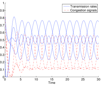
Figure 2: The unmodified dynamics (44) running on the network given in Figure 1 with all link capacities set to $1$ and the utility functions are $\log(1+x)$ and $1-e^{-x}$ for the sources at $1$ and $2$ respectively. In this network the condition (45) holds, and there is oscillatory behaviour which does not decay.

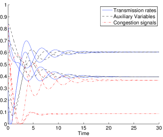
Figure 3: The modified dynamics (48) running on the network given in Figure 1 with all link capacities set to $1$, $\kappa_{j}=1$ for all $j$. The utility functions are $\log(1+x)$ and $1-e^{-x}$ for the sources at $1$ and $2$ respectively. In this network the condition (45) holds, but the modification of the dynamics causes rapid convergence to equilibrium.

Figure 4: A second example network. A single source at $1$ transmits to the destination $7$. It has a choice of two routes.

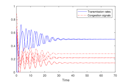
Figure 5: The unmodified dynamics (44) running on the network given in Figure 4 with all link capacities set to $0.5$ and the utility function is $\log(1+x)$. The system is asymptotically stable, but displays transient oscillatory behaviour.

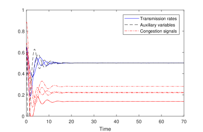
Figure 6: The modified dynamics (48) running on the network given in Figure 4 with all link capacities set to $0.5$, $\kappa_{j}=1$ for all $j$ and the utility function is $\log(1+x)$. The oscillatory behaviour of the unmodified dynamics in Figure 5 is damped, and the system rapidly converges to equilibrium.

V-B4 Numerical examples

In this subsection we present numerical simulations to illustrate the results described above. We consider the two networks in Figure 1 and Figure 4.

In Figure 2 and Figure 3 we use the network in Figure 1 with capacities all set to $1$. The utility functions were chosen as $\log(1+x)$ and $1-e^{-x}$ for the sources at $1$ and $2$ respectively. The parameters $\kappa_{j}$ were all set to $1$. This network satisfies the condition (45) and this is apparent in the oscillating modes of the unmodified dynamics (44), shown in Figure 2, that do not decay. However, when we apply the modified dynamics (48) to this network, we obtain the rapid convergence to the equilibrium shown in Figure 3.

In Figure 5 and Figure 6 we use the network in Figure 4. We take the utility function as $\log(1+x)$, and the capacities all set to $0.5$. The parameters $\kappa_{j}$ were all set to $1$. On this network the original dynamics (44) converge to equilibrium, shown in Figure 5, but there is transient oscillatory behaviour. When we instead implement the modified dynamics (48), shown in Figure 6, we see an improved performance with more rapid convergence and damping of the oscillations.

VI Conclusion

In this paper we considered the problem of convergence to a saddle point of a concave convex function via subgradient dynamics that provide a restriction in an arbitrary convex domain. We showed that despite the nonlinear and non-smooth character of these dynamics, when these have an equilibrium point their $\omega$-limit set is comprised of trajectories that are solutions to only linear ODEs. In particular, we showed that these ODEs are subgradient dynamics on affine subspaces which is a class of dynamics the asymptotic properties of which have been exactly characterized in part I. Various convergence criteria have been deduced from these results that can guarantee convergence to a saddle point. Several examples have also been discussed throughout the manuscript to illustrate the results in the paper.

Appendix A Proofs of the main results

In this appendix we prove the main results of the paper, which are stated in section IV in the main text.

A-A Outline of the proofs

We first give a brief outline of the derivations of the results to improve their readability.

A-A1 Pathwise stability and convex projections

In section A-B of this appendix we prove the results described in subsection IV-B in the main text.

We revisit some of the literature on topological dynamical systems [7], quoting a more general result subsection A-B, from which subsection IV-B is deduced. These results allow us to prove the main result of the subsection, subsection IV-B, using the fact that the convex projection term cannot break the isometry property of the flow on the $\omega$-limit set.

A-A2 Subgradient method

In sections A-C, A-D in this appendix we prove the results in subsections IV-C, IV-D, respectively, in the main text using the results in subsection IV-B.

A-B Convergence to a flow of isometries

In this section we provide the proofs of subsection IV-B and subsection IV-B.

We begin by revisiting the literature on topological dynamical systems, in which a type of incremental stability is studied, and show how this leads to an invariance principle for pathwise stability.

Definition (Equicontinuous semi-flow).

We say that a flow (resp. semi-flow) $(\phi,X,\rho)$ is equicontinuous if for any $x(0)\in X$ and $\varepsilon>0$ there is a $\delta=\delta(x(0),\varepsilon)$ such that if $\rho(x^{\prime}(0),x(0))<\delta$ then

$$\rho(x(t),x^{\prime}(t))\leq\varepsilon\text{ for all }t\in\mathbb{R}\text{ (resp. $\mathbb{R}_{+}$)}.$$ (50)

Remark .

In the control literature equicontinuity of a semi-flow would correspond to ‘semi-global non-asymptotic incremental stability’, but we shall keep the term equicontinuity for brevity and consistency with [7].

Definition (Uniformly almost periodic flow).

We say that a flow $(\phi,X,\rho)$ is uniformly almost periodic if for any $\varepsilon>0$ there is a syndetic set $A\subseteq\mathbb{R}$, (i.e. $\mathbb{R}=A+B$ for some compact set $B\subseteq\mathbb{R}$), for which

$$\rho(\phi(t,x),x)\leq\varepsilon\text{ for all }t\in A,x\in X.$$ (51)

For the readers convenience we reproduce the results, [7, Theorem 8] and [12, Proposition 4.4.], that we will use.

Theorem (G. Della Riccia [7]).

Let $(\phi,X,\rho)$ be an equicontinuous semi-flow and let $X$ be either locally compact or complete. Let $\Omega$ be its $\omega$-limit set. Then $(\phi,\Omega,\rho)$ is an equicontinuous semi-flow of homeomorphisms of $\Omega$ onto $\Omega$. This generates an equicontinuous flow.

The backwards flow given by subsection A-B is only unique on $\Omega$, (see subsection IV-B which also applies here).

Proposition (R. Ellis [12]).

Let $(\phi,X,\rho)$ be a flow, with $X$ compact. Then the following are equivalent:

1. The flow is equicontinuous.

2. The flow is uniformly almost periodic.

In our case we study pathwise stability which is a particular form of equicontinuity. We prove stronger results in this special case.

Proof of subsection IV-B.

By subsection A-B $(\phi,\Omega,d)$ is an equicontinuous flow with an equilibrium point $\mathbf{\bar{z}}$. Let $R>0$ be arbitrary, and define

$$Y_{R}=\left\{\mathbf{z}(0)\in\Omega:\sup_{t\in\mathbb{R}}d(\mathbf{z}(t),\mathbf{\bar{z}})\leq R\right\}.$$ (52)

As the flow is equicontinuous, $Y_{R}$ is a closed bounded subset of $\mathbb{R}^{n+m}$ and hence compact, and moreover, the union of the sets $Y_{R}$ over $R\geq 0$ is $\Omega$. By subsection A-B the flow $(\phi,Y_{R},d)$ is uniformly almost periodic. By pathwise stability, $d:Y_{R}\times Y_{R}\to\mathbb{R}$ is a non-increasing along the direct product flow, and is a continuous function on a compact set. Hence we have the inequality, for any two points $\mathbf{z}(0),\mathbf{z}^{\prime}(0)\in Y_{R}$,

$$\lim_{t\to-\infty} d(\mathbf{z}(t),\mathbf{z}^{\prime}(t))=\sup_{t\in\mathbb{R}}d(\mathbf{z}(t),\mathbf{z}^{\prime}(t))$$ (53)

$$\geq\inf_{t\in\mathbb{R}}d(\mathbf{z}(t),\mathbf{z}^{\prime}(t))=\lim_{t\to\infty}d(\mathbf{z}(t),\mathbf{z}^{\prime}(t)).$$

We claim that the two limits are equal. Indeed, by uniform almost periodicity there are sequences $t_{n}\to\infty$ and $t_{n}^{\prime}\to-\infty$ as $n\to\infty$ for which

$$0=\lim_{n\to\infty}d(\mathbf{z}(t_{n}),\mathbf{z}(0))=\lim_{n\to\infty}d(\mathbf{z}(t_{n}^{\prime}),\mathbf{z}(0))$$ (54)

and the analogous limits hold for $\mathbf{z}^{\prime}$ for the same sequences $t_{n},t_{n}^{\prime}$. Hence, by continuity of $d$, we have

$$\lim_{t\to-\infty}d(\mathbf{z}(t),\mathbf{z}^{\prime}(t))=d(\mathbf{z}(0),\mathbf{z}^{\prime}(0))=\lim_{t\to\infty}d(\mathbf{z}(t),\mathbf{z}^{\prime}(t)).$$ (55)

Hence $d(\mathbf{z}(t),\mathbf{z}^{\prime}(t))$ is constant. By picking $R$ big enough, this holds for any $\mathbf{z}(0),\mathbf{z}^{\prime}(0)\in\Omega$, which completes the proof that the sub-semi-flow generates a flow of isometries.

It remains to show that $\Omega$ is convex. To this end let $\mathbf{z}(t),\mathbf{z}^{\prime}(t)$ be two trajectories of $(\phi,\Omega,d)$. Let that $\lambda\in(0,1)$ and define $\mathbf{z}^{\prime\prime}(t)=\lambda\mathbf{z}(t)+(1-\lambda)\mathbf{z}^{\prime}(t)$. By the same argument as used in the proof of [21, Proposition 32] we deduce that $\mathbf{z}^{\prime\prime}(t)$ is a trajectory of the original semi-flow, but (as argued above) by uniform almost periodicity of $(\phi,\Omega,d)$ we have a sequence of times $t_{n}\to\infty$ for which $d(\mathbf{z}(t_{n}),\mathbf{z}(0))\to 0$ as $n\to\infty$ and the same limit for $\mathbf{z}^{\prime}(t)$. Hence $d(\mathbf{z}^{\prime\prime}(t_{n}),\mathbf{z}^{\prime\prime}(0))\to 0$ also, showing that $\mathbf{z}^{\prime\prime}(0)$ is in the $\omega$-limit set. ∎

We now use the isometry property together with the geometry of the convex projection term to obtain the key result of this section, subsection IV-B, which states that the limiting dynamics of a pathwise stable ODE restricted to a convex set $K$ have $C^{1}$ smooth vector field and lie inside one of the faces of $K$.

To prove the theorem we will make use of a simple lemma on faces of convex sets.

Lemma .

Let $K\subseteq\mathbb{R}^{n}$ be non-empty closed and convex and $A\subseteq K$. Let $F$ be the minimal face of $K$ containing $A$, (see subsubsection II-A3), then $\operatorname*{relint}(F)$ intersects $\operatorname*{Conv}A$.

The statement of this lemma and the idea behind its proof are illustrated by Figure 7.

Figure 7: This figure illustrates the claim of subsection A-B. The triangle $F$ is the minimal face containing the convex set $A$ (shaded region). If $A$ intersects two subfaces of $F$, then, as shown, to be convex it must also intersect the relative interior of $F$.

Proof.

As faces are convex, the minimal face containing $A$ is the same as the minimal face containing $\operatorname*{Conv}A$. So we are free to assume without loss of generality that $A$ is convex. Assume for a contradiction that $A\cap\operatorname*{relint}(F)=\emptyset$. Define the set $\mathcal{F}$ as

$$\{C:C\text{ is a proper face of }F\text{ and }A\cap(\operatorname*{relint}C)\neq\emptyset\}.$$

Note that every point in the relative boundary of $F$ lies in the relative interior of some proper face of $F$ by property (e) below subsubsection II-A3. This implies that $\mathcal{F}$ is not empty. Now, either there is a face $C$ in $\mathcal{F}$ that contains all other faces in $\mathcal{F}$, or there are two faces $F_{1},F_{2}\in\mathcal{F}$ such that there is no face $F_{3}\in\mathcal{F}$ containing both $F_{1}$ and $F_{2}$. In the first case, $C$ is a face containing $A$ that is strictly contained in $F$, contradicting minimality of $F$. In the second case let $x_{i}\in(\operatorname*{relint}F_{i})\cap A$ for $i=1,2$, (note that $x_{1}\neq x_{2}$ by property (e) of faces), and let $x_{3}$ be some point in the open line segment between $x_{1}$ and $x_{2}$. By convexity of $A$, $x_{3}\in A$. Hence $x_{3}$ lies in $\operatorname*{relint}(F_{3})$ for some face $F_{3}$, and $F_{3}\in\mathcal{F}$, as otherwise $x_{3}$ would lie in $\operatorname*{relint}(F)$ contradicting the assumption that $(\operatorname*{relint}F)\cap A=\emptyset$. We claim that $F_{3}$ contains both $F_{1}$ and $F_{2}$, a contradiction. Indeed, first we note that $x_{1},x_{2}\in F_{3}$ by property (ii) in subsubsection II-A3 as $x_{3}\in F_{3}$. Then, as $F_{i}$ is convex and $x_{i}\in\operatorname*{relint}(F_{i})$, $F_{i}$ can be written as the union of line segments which have $x_{i}$ as an interior point (i.e. not an end point). But each of these line segments touches $F_{3}$ at $x_{i}$, so by subsubsection II-A3(ii) each lies entirely within $F_{3}$. ∎

Proof of subsection IV-B.

From the text above the statement of the Corollary we have that all trajectories of the semiflow converge to its $\omega$-limit set (denoted as $\Omega$). Also from subsection IV-B we have that $(\phi,\Omega,d)$ defines a flow of isometries.

Convergence to $\Omega$ can now be strengthened to convergence to a solution in $\Omega$ using the same arguments as in the proof of [21, Corollary 11] with set $\mathcal{S}$ replaced with $\Omega$. ∎

Proof of subsection IV-B.

Step 1: Identification of the limiting equation. First, by subsection IV-B and subsection IV-B $(\phi,\Omega,d)$ is a flow of isometries. Now let $F$ be the minimal face that contains $\Omega$, i.e. the intersection of all faces that contain $\Omega$, and $N_{F}$ be its normal cone (in step 2 of the proof we will identify this face more precisely). We note that the vector field in (15) must be directed parallel to $V$, as otherwise trajectories would leave $F$, contradicting $\Omega\subseteq F$.

It is sufficient to show that if $\mathbf{z}=\mathbf{z}(0)\in\Omega$ with $\mathbf{n}(t)=\mathbf{P}_{N_{K}(\mathbf{z}(t))}(\mathbf{f}(\mathbf{z}(t)))$ then $\mathbf{n}(t)$ is orthogonal to $F$. If $\mathbf{z}(t)\in\operatorname*{relint}K$ then $N_{K}(\mathbf{z}(t))=N_{F}$ and the orthogonality holds. Otherwise $\mathbf{z}(t)$ lies in the relative boundary of $F$.

As each solution of the differential equation (15) holds only for almost all times $t$ and we wish to consider an uncountably infinite family of solutions, we run the risk of taking an uncountable union of sets of measure zero, (which does not necessarily have zero measure). Avoiding this makes the proof technical. To better communicate the idea of the proof, we shall first give the proof that would work if the differential equations held for all times $t$.

Step 1.1: Heuristic (unrigorous) proof.

Let $C=\operatorname*{Conv}\Omega$, then, by the definition of a face, $\Omega\subseteq F$ implies that $C\subseteq F$. From subsection A-B and the minimality of $F$ we deduce that $C$ must intersect $\operatorname*{relint}F$. Thus there are $\mathbf{x}(0),\mathbf{y}(0)\in\Omega$ and $\lambda\in(0,1)$ with $\mathbf{w}=\lambda\mathbf{x}(0)+(1-\lambda)\mathbf{y}(0)\in\operatorname*{relint}F$. Set $W=\frac{1}{2}|\mathbf{x}(t)-\mathbf{z}(t)|^{2}$. By the isometry property of the flow we know that $\dot{W}=0$ at $t$. We also have,

$$\dot{W}(t) =(\mathbf{x}(t)-\mathbf{z}(t))^{T}(\mathbf{\dot{x}}(t)-\mathbf{\dot{z}}(t))$$ (56)

$$=(\mathbf{x}(t)-\mathbf{z}(t))^{T}(\mathbf{f}(\mathbf{x}(t))-\mathbf{f}(\mathbf{z}(t)))+$$

$$\quad-(\mathbf{x}(t)-\mathbf{z}(t))^{T}\mathbf{P}_{N_{K}(\mathbf{x}(t))}(\mathbf{f}(\mathbf{x}(t)))+$$

$$\quad+(\mathbf{x}(t)-\mathbf{z}(t))^{T}\mathbf{P}_{N_{K}(\mathbf{z}(t))}(\mathbf{f}(\mathbf{z}(t))).$$

The first term in (56) is non-positive due to the assumption that the ODE satisfies (15). The other two terms are non-positive due to the definition of the normal cone. Hence $\dot{W}=0$ implies that $(\mathbf{x}-\mathbf{z})^{T}\mathbf{n}=0$. Similarly we obtain $(\mathbf{y}-\mathbf{z})^{T}\mathbf{n}=0$. Taking a convex combination of these equalities, we obtain

$$(\mathbf{w}-\mathbf{z})^{T}\mathbf{n}=\lambda(\mathbf{x}-\mathbf{z})^{T}\mathbf{n}+(1-\lambda)(\mathbf{y}-\mathbf{z})^{T}\mathbf{n}=0+0=0$$ (57)

and as $\mathbf{w}$ is in the relative interior of $F$ this implies that $\mathbf{n}$ is orthogonal to $F$.

Step 1.2: Rigorous proof. We now give the fully rigorous proof. We must show that the set of times $t$ when $\mathbf{n}(t)$ is not orthogonal to $F$ is of measure zero. Let $\Omega^{\prime}$ be a countable dense subset of $\Omega$ that contains $\mathbf{z}(0)$. By invariance of $\Omega$ under the flow $\phi$, the set $\phi(t,\Omega^{\prime})=\{\phi(t,\mathbf{x}):\mathbf{x}\in\Omega^{\prime}\}$ is also dense in $\Omega$ for any $t\in\mathbb{R}$. Then the set

$$A=\{t \in[0,\infty):\exists\mathbf{x}(0)\in\Omega^{\prime}\text{ such that }$$ (58)

$$\dot{\mathbf{x}}(t)\neq\mathbf{f}(\mathbf{x}(t))-\mathbf{P}_{N_{K}(\mathbf{x}(t))}(\mathbf{f}(\mathbf{x}(t)))\}$$

is the countable union of measure zero sets, and is hence of measure zero. From the isometry property and by considering $W(t)=\frac{1}{2}|\mathbf{x}(t)-\mathbf{z}(t)|^{2}$ with $\mathbf{x}(0)\in\Omega^{\prime}$, it follows that $(\mathbf{x}(t)-\mathbf{z}(t))^{T}\mathbf{n}(t)=0$ for all $\mathbf{x}(0)\in\Omega^{\prime}$ and $t\in[0,\infty)\setminus A$. Thus, for $t\in[0,\infty)\setminus A$, $(\mathbf{x}-\mathbf{z}(t))^{T}\mathbf{n}(t)=0$ for all $\mathbf{x}$ in a dense subset of $\Omega$, and hence for any $\mathbf{x}\in\Omega$. The proof now follows as step 1.1. above.

Step 2: Identification of the limiting face. Finally we will show that the face $F$ defined above is in fact the minimal face $F^{\prime}$ containing the equilibrium points of the semi-flow $(\phi,K,d)$. We argue by contradiction. If $F\neq F^{\prime}$ then there must be some trajectory $\mathbf{z}(t)$ in $\Omega$ and a time $t_{0}$ with $\mathbf{z}(t_{0})\in F\setminus F^{\prime}$. For $T>0$ we define $\mathbf{z}(t;T)=\frac{1}{2T}\int^{T}_{-T}\mathbf{z}(t+s)\,ds$. For any finite $T$ this is a convex combination of trajectories in $\Omega$, and as $\Omega$ is convex by subsection IV-B, $t\mapsto\mathbf{z}(t;T)$ is a trajectory in $\Omega$. Next, as the semi-flow is uniformly almost periodic due to subsection A-B the trajectory $\mathbf{z}(t)$ is an almost periodic function. Therefore, the limit $T\to\infty$ of $\mathbf{z}(t;T)$ exists (see e.g. [12]), and this limit is clearly a constant ($\mathbf{z}^{\prime}$ say) independent of $t$. As $\Omega$ is closed, $\mathbf{z}^{\prime}\in\Omega$ and being a constant, is an equilibrium point of the semi-flow.

To obtain a contradiction we argue that $\mathbf{z}^{\prime}\not\in F^{\prime}$ which is impossible as $F^{\prime}$ contains all equilibrium points. Indeed, this follows as the trajectory $\mathbf{z}(t)$, being almost periodic and passing through $\mathbf{z}(t_{0})\in F\setminus F^{\prime}$ spends a positive proportion of its time in $F\setminus F^{\prime}$. Therefore, there is a $\delta>0$ such that for any sufficiently large $T$, the average $\mathbf{z}(t;T)$ satisfies $d(\mathbf{z}(t;T),F)\geq\delta$ and this property carries over to the limit $\mathbf{z}^{\prime}$. ∎

A-C Subgradient method

In this section we give the proofs of the results of subsection IV-C.

Proof of subsection IV-C.

We apply subsection IV-B, noting that $\mathbf{f}(\mathbf{z})$ in (9) satisfies the inequality in (15) [40], [17].

Case (i). This follows directly from subsection IV-B.

Case (ii). As $F$ must contain all $K$-restricted saddle points, it must contain a point in the interior of $K$. The only such face is $K$ itself whose affine span is $\mathbb{R}^{n+m}$ (as $K$ has non-empty interior) which has normal cone $\{\mathbf{0}\}$. Therefore in case (ii) (16) becomes the gradient method (8) and (18) holds.

The convexity and isometry properties of $\Omega$ stated follow from subsection IV-B. ∎

A-D A general convergence criterion

In this section we give the proofs of subsection IV-D.

Proof of subsection IV-D.

By subsection IV-C(i) any solution $\mathbf{z}(t)$ in the $\omega$-limit set of the subgradient method on $K$ solves (17). By using $\mathbf{\Pi}$, the orthogonal projection matrix onto the orthogonal complement of $N_{V}$, the ODE (17) can be written as (12). Noting also the isometry property of the $\omega$-limit set, we have by subsection IV-A (in Appendix IV-A), that $\mathbf{z}(t)$ satisfies (36) and (37) for all $t\in\mathbb{R}$ and $r\in[0,1]$. Therefore, if there are no non-constant trajectories of the subgradient method on $K$ satisfying these conditions then the $\omega$-limit set consists only of equilibrium points and the subgradient method on $K$ is globally convergent. ∎

Proof of subsection IV-D.

This follows from subsection IV-C and subsection IV-A using the arguments in the proof of subsection IV-D. ∎

Appendix B Proofs of the results in section V

B-A Modification methods

Proof of subsubsection V-A4:
We prove convergence of each modification method in turn.

B-A1 Auxiliary variables method

Proposition .

Let (38) hold, and assume that there exists a $K^{\prime}$-restricted saddle point. Then the subgradient method (9) on $K^{\prime}$ applied to $\varphi^{\prime}$ is globally convergent.

Proof.

We prove global convergence to an equilibrium point by making use of Theorem IV-D. In particular, we show that the only solutions of the subgradient method applied to $\phi^{\prime}$, which satisfy both (36) and (37), are equilibrium points.

Without loss of generality, we assume, by a translation of coordinates, that $\mathbf{\bar{z}}^{\prime}=(M\bar{x},\bar{x},\bar{y})=\mathbf{0}$ is an equilibrium point. Since the auxiliary variables are unconstrained the orthogonal complement of $N_{V}$ in Theorem IV-D is a subspace of the form $\mathbb{R}^{n^{\prime}}\times V^{\prime}$ where $V^{\prime}\subseteq\mathbb{R}^{n+m}$ is an affine subspace.

Let $\mathbf{\Pi}$ be the orthogonal projection matrix onto the subspace $\mathbb{R}^{n^{\prime}}\times V^{\prime}$. We decompose $\mathbf{\Pi}$ on $\mathbb{R}^{n^{\prime}}\times\mathbb{R}^{n+m}$ as

$$\mathbf{\Pi}=\begin{bmatrix}I&\mathbf{0}\\ \mathbf{0}&\mathbf{\Pi}^{\prime}\end{bmatrix}.$$ (59)

Now let $\mathbf{z}(t)=(x^{\prime}(t),x(t),y(t))$ be a solution of the modified subgradient method that satisfies (36) and (37), and let $(\tilde{x}(t),\tilde{y}(t))=\mathbf{\Pi}^{\prime}(x(t),y(t))$. The remainder of the proof is carried out in three steps.

Step 1: $x^{\prime}(t)$ is constant. By the form of $\mathbf{A}(\mathbf{0})$ in (36) we deduce that $\dot{x}^{\prime}(t)=0$.

Step 2: $\tilde{x}(t)$ and $\tilde{y}(t)$ are constant. From the condition (37) that ${\color[rgb]{0,0,0}{\mathbf{\Pi}}}\mathbf{B}(r\mathbf{z})\mathbf{\Pi}\mathbf{z}=0$ for $r\in[0,1]$, we have that

$$0=\mathbf{z}^{T}\mathbf{\Pi}\mathbf{B}(r\mathbf{z})\mathbf{\Pi}\mathbf{z}=u^{T}\psi_{uu}u+\tilde{x}^{T}\varphi_{xx}\tilde{x}-\tilde{y}^{T}\varphi_{yy}\tilde{y}$$ (60)

where $\psi_{uu}$ is the Hessian matrix of $\psi$ evaluated at $u=M\tilde{x}-x^{\prime}$. As each term is non-positive and $\psi$ is strictly concave we deduce that $M\tilde{x}-x^{\prime}=0$ and $\tilde{x}\in\ker(\varphi_{xx}(\mathbf{0}))$. Thus $M\tilde{x}(t)$ is constant. By the condition that $\ker(M)\cap\ker(\varphi_{xx})=\{0\}$ we deduce that $\tilde{x}(t)$ is constant. Then the form of $\mathbf{A}(\mathbf{0})$ allows us to deduce that $\tilde{y}(t)$ is also constant.

Step 3: $x(t)$ and $y(t)$ are constant. The vector field in (36) is orthogonal to $\ker(\mathbf{\Pi})$, so that $(\tilde{x}(t),\tilde{y}(t))$ being constant implies that $(x(t),y(t))$ are constant.

This completes the proof of convergence to an equilibrium point of the subgradient method applied to $\phi^{\prime}$ . ∎

B-A2 Penalty function method

Proposition .

Let $K\subseteq\mathbb{R}^{n+m}$ be non-empty closed and convex as in (1a). Let (39), (40) hold, and assume that there exists a $K$-restricted saddle point. Then the subgradient method (9) on $K$ applied to $\varphi^{\prime}$ is globally convergent.

Proof.

Without loss of generality, we may assume by a translation of coordinates that $\mathbf{0}$ is a $K$-restricted saddle point. We apply subsection IV-D and let $F,V,\mathbf{\Pi}$ be as in subsection IV-D and $\mathbf{z}(t)=(x(t),y(t))$ be a trajectory of the subgradient method on $K$ satisfying (36) and (37) for all $t\in\mathbb{R}$ and $r\in[0,1]$. Define $(\tilde{x}(t),\tilde{y}(t))=\tilde{\mathbf{z}}(t)=\mathbf{\Pi}\mathbf{z}(t)$. We compute that

$$\mathbf{A}(\mathbf{0})=\begin{bmatrix}0&g_{x}(0)^{T}\\ -g_{x}(0)&0\end{bmatrix}.$$ (61)

Step 1: $g_{x}(0)\tilde{x}(t)=0$.

The condition (37) implies that the following expression is zero for all $s\in[0,1]$,

$$\tilde{\mathbf{z}}^{T}\mathbf{B}(s\mathbf{z}){\color[rgb]{0,0,0}\tilde{\mathbf{z}}}=\tilde{x}^{T}\varphi_{xx}\tilde{x}+[g_{x}\tilde{x}]^{T}\psi_{uu}[g_{x}\tilde{x}]+\psi_{u}(\tilde{x}^{T}g_{xx}\tilde{x})$$ (62)

where $\varphi_{xx}$ is evaluated at $s\mathbf{z}$, with $g_{x},g_{xx}$ at $sx$, and $\psi_{uu},\psi_{u^{k}}$ at $u=g(sx)$, and where $x^{T}g_{xx}x$ is the vector with $i$th component $x^{T}g^{i}_{xx}x$ where $g=[g^{1},\dotsc,g^{m}]^{T}$. All the terms are non-positive by the assumptions on $\psi$ and $\varphi$. Strict concavity of $\psi$ and that (62) vanishes for all $s\in[0,1]$ implies that $g_{x}(sx)\tilde{x}=0$ for all $s\in[0,1]$. In particular $g_{x}(0)\tilde{x}(t)=0$.

Step 2: $\tilde{x}(t)$ is constant.

Let $\mathbf{\Pi}$ be decomposed on $\mathbb{R}^{n}\times\mathbb{R}^{m}$ as

$$\mathbf{\Pi}=\begin{bmatrix}\Pi_{11}&\Pi_{12}\\ \Pi_{21}&\Pi_{22}\end{bmatrix}.$$ (63)

Then $\tilde{x},\tilde{y}$ satisfy

$$\dot{\tilde{x}} =\Pi_{11}g_{x}(0)^{T}\tilde{y} \quad\dot{\tilde{y}} =-\Pi_{21}g_{x}(0)^{T}\tilde{y}.$$ (64)

Taking the time derivative of $g_{x}(0)\tilde{x}=0$ we obtain $g_{x}(0)\Pi_{11}g_{x}(0)^{T}\tilde{y}=0$. As $\Pi_{11}$ is positive semi-definite, $\ker(g_{x}(0)\Pi_{11}g_{x}(0)^{T})=\ker(\Pi_{11}g_{x}(0)^{T})$, and hence $\dot{\tilde{x}}=\Pi_{11}g_{x}(0)^{T}\tilde{y}=0$ and $\tilde{x}(t)$ is constant.

Step 3: $\tilde{y}(t)$ is constant.

The relation $\mathbf{\Pi}\dot{\tilde{\mathbf{z}}}=\dot{\tilde{\mathbf{z}}}$ implies that $\Pi_{11}\dot{\tilde{x}}+{\color[rgb]{0,0,0}\Pi_{12}}\dot{\tilde{y}}=\dot{\tilde{x}}=0$ and $0=\Pi_{12}\dot{\tilde{y}}=-\Pi_{12}\Pi_{21}g_{x}(0)^{T}\tilde{y}$. Therefore, again, as $\Pi_{12}\Pi_{21}$ is positive semi-definite we have $\tilde{y}^{T}g_{x}(0)\Pi_{12}\Pi_{21}g_{x}(0)^{T}\tilde{y}=0$ and $\Pi_{21}g_{x}(0)^{T}\tilde{y}=0=-\dot{\tilde{y}}$, which implies $\tilde{y}$ is constant.

The fact that $x(t)$, $y(t)$ are constant can be deduced as in Step 3 of the proof of subsubsection B-A1. ∎

B-A3 Constraint modification method

We first consider the case without constraints. The proof below shows that the method works by disrupting the linear structure of the oscillating solutions by changing $\mathbf{A}(\mathbf{z})$ to ensure it is not equal to $\mathbf{A}(\mathbf{0})$, (where $\mathbf{0}$ is a saddle).

Proposition .

Let (41) hold and $\bar{\mathcal{S}}\neq\emptyset$. Then $\mathcal{S}=\bar{\mathcal{S}}$ and the gradient method (8) applied to $\varphi^{\prime}$ is globally convergent.

Proof.

Without loss of generality we may assume that $\mathbf{0}$ is a saddle point of $\varphi$. We use the classification of $\mathcal{S}$ given by [21, Theorem 12] and use the notation therein. We first compute,

$$\mathbf{A}(\mathbf{z})=\begin{bmatrix}0&(\psi_{g}g_{x})^{T}\\ -\psi_{g}g_{x}&0\end{bmatrix}.$$ (65)

Let $\mathbf{z}(t)=(x(t),y(t))\in\mathcal{S}$ then we have

$$0 =\frac{d}{ds}[(\psi_{g}^{i}(g(sx))^{T}g_{x}(sx)x]_{s=0}\text{ for }i=1,\dotsc,m$$ (66)

Then by applying the chain rule we obtain

$$0=[g_{x}(0)x]^{T}\psi^{i}_{gg}(0)[g_{x}(0)x]+\psi^{i}_{g}(0)^{T}(x^{T}g_{xx}(0)x),$$ (67)

where $x^{T}g_{xx}(0)x$ is the vector with components $x^{T}g^{i}_{xx}x$ where $g=[g^{1},\dotsc g^{m}]^{T}$. All the terms are non-positive due to the assumptions on $\psi$ and $g$. As $\psi_{gg}^{i}<0$ we have $g_{x}(0)x=0$. Hence $\dot{y}=0$ and therefore $y$ is constant. As $|x|^{2}+|y|^{2}$ is also constant this means that $\dot{x}$ is zero. Therefore $\mathcal{S}=\bar{\mathcal{S}}$ and the gradient method is globally convergent. ∎

Now we extend the stability to the subgradient method on sets which have a product structure, by making use of subsection IV-C.

Corollary .

Let $K\subseteq\mathbb{R}^{n+m}$ be non-empty closed and convex as in (1a). Let (41) hold and there be a $K$-restricted saddle point. Then the subgradient method (9) on $K$ applied to $\varphi^{\prime}$ is globally convergent.

Proof.

By subsection IV-C it suffices to prove that the subgradient method on $\operatorname*{aff}(F)$ is globally convergent, where $F$ is an arbitrary face of $K$ that contains a $K$-restricted saddle point $\mathbf{\bar{z}}$. By translation of coordinates we may assume that $\mathbf{\bar{z}}=\mathbf{0}$. By the product structure of $K$, $V=\operatorname*{aff}(F)$ must also decompose into $V=V_{x}\times V_{y}$ with $V_{x}\subseteq\mathbb{R}^{n}$ and $V_{y}\subseteq\mathbb{R}^{m}$ affine subspaces. Let the orthogonal projection matrices onto $V_{x},V_{y}$, which exist as $(0,0)\in V_{x}\times V_{y}$, be $P,Q$ respectively. Then the subgradient method on $V$, satisfies, for $(x,y)\in V$,

$$\dot{x} =P\varphi^{\prime}_{x}=\varphi^{V}_{x}, \dot{y} =-Q\varphi^{\prime}_{y}=-\varphi^{V}_{y}$$ (68)

where $\varphi^{V}(x,y):=\varphi(Px,Qy)$. By a rotation of coordinate bases we may assume that $V_{x}=\mathbb{R}^{n^{\prime}}\times\{0\}$ and $V_{y}=\mathbb{R}^{m^{\prime}}\times\{0\}$ for some $n^{\prime}\leq n$ and $m^{\prime}\leq m$. Then $\varphi^{V}:\mathbb{R}^{n^{\prime}}\times\mathbb{R}^{m^{\prime}}\to\mathbb{R}$ is of the form (41) and subsubsection B-A3 gives convergence. ∎

B-B Multi-path congestion control

Proof of subsubsection V-B2.

The if claim follows directly from the discussion preceding the proposition. For the only if we explicitly construct a trajectory that does not converge. Let $u$ satisfy (45), then it can be directly verified that

$$\mathbf{z}(t)=\bar{\mathbf{z}}+ce^{t\mathbf{A}(\bar{\mathbf{z}})}\begin{bmatrix}u\\ -Au\end{bmatrix}$$

is a solution (for any $c>0$) of the unconstrained gradient method (8) applied to $\varphi$. By taking $c$ small enough using the fact that $\bar{\mathbf{z}}>0$ (and the skew-symmetry of $\mathbf{A}(\bar{\mathbf{z}})$) we can ensure that $\mathbf{z}(t)>0$ for all $t\in\mathbb{R}$, and hence $\mathbf{z}(t)$ is also a solution of the subgradient dynamics (44). ∎

References

- [1] K. J. Arrow, L. Hurwicz, and H. Uzawa. Studies in linear and non-linear programming. Standford University Press, 1958.
- [2] S. Boyd, N. Parikh, E. Chu, B. Peleato, and J. Eckstein. Distributed optimization and statistical learning via the alternating direction method of multipliers. Found. Trends Mach. Learn., 3(1):1–122, January 2011.
- [3] S. Boyd and L. Vandenberghe. Convex Optimization. Cambridge University Press, New York, NY, USA, 2004.
- [4] B. Brogliato, A. Daniilidis, C. Lemarechal, and V. Acary. On the equivalence between complementarity systems, projected systems and differential inclusions. Systems & Control Letters, 55(1):45–51, 2006.
- [5] A. Cherukuri, E. Mallada, and J. Cortés. Asymptotic convergence of constrained primal–dual dynamics. Systems & Control Letters, 87:10–15, 2016.
- [6] A. Cherukuri, E. Mallada, S. Low, and J. Corteés. The role of convexity on saddle-point dynamics: Lyapunov function and robustness. arXiv preprint arXiv:1608.08586, 2016.
- [7] G. Della Riccia. Equicontinuous semi-flows (one-parameter semi-groups) on locally compact or complete metric spaces. Mathematical systems theory, 4(1):29–34, 1970.
- [8] E. Devane, A. Kasis, M. Antoniou, and I. Lestas. Primary frequency regulation with load-side participation Part II: Beyond passivity approaches. IEEE Transactions on Power Systems, 32(5):3519–3528, 2017.
- [9] E. Devane, A. Kasis, C. Spanias, M. Antoniou, and I. Lestas. Distributed frequency control and demand-side management. Smarter Energy: From Smart Metering to the Smart Grid, pages 245–268, 2016.
- [10] E. Devane and I. Lestas. Stability and convergence of distributed algorithms for the OPF problem. In 52nd IEEE Conference on Decision and Control, December 2013.
- [11] F. Dörfler, J. Simpson-Porco, and F. Bullo. Breaking the hierarchy: Distributed control and economic optimality in microgrids. IEEE Transactions on Control of Network Systems, 3(3):241–253, 2016.
- [12] R. Ellis. Lectures on topological dynamics. Mathematics lecture note series. W. A. Benjamin, 1969.
- [13] D. Feijer and F. Paganini. Stability of primal-dual gradient dynamics and applications to network optimization. Automatica, 46(12):1974–1981, 2010.
- [14] W.J. Feng, L. Wang, and Q.G. Wang. A family of multi-path congestion control algorithms with global stability and delay robustness. Automatica, 50(12):3112 – 3122, 2014.
- [15] R.M. Freund. Penalty and barrier methods for constrained optimization. Lecture notes for nonlinear programming. MIT., 2004.
- [16] D. Gabay and B. Mercier. A dual algorithm for the solution of nonlinear variational problems via finite element approximation. Computers and Mathematics with Applications, 2(1):17–40, 1976.
- [17] R. Goebel. Stability and robustness for saddle-point dynamics through monotone mappings. Systems & Control Letters, 108:16–22, 2017.
- [18] P.M. Gruber and J.M. Wills. Handbook of Convex Geometry. Convex Geometry. North-Holland, 1993.
- [19] T. Holding and I. Lestas. Stability and instability in primal-dual algorithms for multi-path routing. In 54th IEEE Conference on Decision and Control, December 2015.
- [20] T. Holding and I. Lestas. On the emergence of oscillations in distributed resource allocation. Automatica, 85:22–33, 2017.
- [21] T. Holding and I. Lestas. Stability and instability in saddle point dynamics - Part I. arXiv preprint arXiv:1707.07349, 2017.
- [22] L. Hurwicz. The design of mechanisms for resource allocation. The American Economic Review, 63(2):1–30, May 1973.
- [23] K. Kar, S. Sarkar, and L. Tassiulas. Optimization based rate control for multipath sessions. Technical report, Univ. of Maryland, Inst. Systems Research, 2001. http://hdl.handle.net/1903/6225.
- [24] A. Kasis, E. Devane, C. Spanias, and I. Lestas. Primary frequency regulation with load-side participation Part I: Stability and Optimality. IEEE Transactions on Power Systems, 32(5):3505–3518, 2017.
- [25] A. Kasis, N. Monshizadeh, E. Devane, and I. Lestas. Stability and optimality of distributed secondary frequency control schemes in power networks. arXiv preprint arXiv:1703.00532, 2017.
- [26] F. Kelly, A. Maulloo, and D. Tan. Rate control in communication networks: shadow prices, proportional fairness and stability. Journal of the Operational Research Society, 49(3):237–252, March 1998.
- [27] H. K. Khalil. Nonlinear Systems. Prentice Hall, 2002.
- [28] G. Lee and J. Choi. A survey of multipath routing for traffic engineering.
- [29] I. Lestas and G. Vinnicombe. Combined control of routing and flow: a multipath routing approach. In 43rd IEEE Conference on Decision and Control, December 2004.
- [30] N. Li, C. Zhao, and L. Chen. Connecting automatic generation control and economic dispatch from an optimization view. IEEE Transactions on Control of Network Systems, 3(3):254–264, 2016.
- [31] X. Lin and N.B. Shroff. Utility maximization for communication networks with multipath routing. IEEE Transactions on Automatic Control, 51(5):766–781, 2006.
- [32] S. H. Low and D. E. Lapsley. Optimization flow control I: basic algorithm and convergence. IEEE/ACM Transactions on Networking, 7(6):861–874, 1999.
- [33] J. Lygeros, K. H. Johansson, S. N. Simić, J. Zhang, and S. S. Sastry. Dynamical properties of hybrid automata. IEEE Transactions on Automatic Control, 48(1):2–17, 2003.
- [34] E. Mallada, C. Zhao, and S. Low. Optimal load-side control for frequency regulation in smart grids. IEEE Transactions on Automatic Control, 62(3):6294–6309, 2017.
- [35] James D Meiss. Differential dynamical systems, volume 14. Siam, 2007.
- [36] A. Nedić and A. Ozdaglar. Subgradient methods for saddle-point problems. Journal of Optimization Theory and Applications, 142(1):205–228, 2009.
- [37] F. Paganini and E. Mallada. A unified approach to congestion control and node-based multipath routing. IEEE/ACM Transactions on Networking, 17(5):1413–1426, October 2009.
- [38] D. Richert and J. Cortés. Robust distributed linear programming. IEEE Transactions on Automatic Control, 60(10):2567–2582, 2015.
- [39] R. T. Rockafellar. Saddle-points and convex analysis. Differential games and related topics, 109, 1971.
- [40] R. T. Rockafellar. Convex analysis. Princeton University Press, 2nd edition, 1972.
- [41] J.S. Shamma and G. Arslan. Dynamic fictitious play, dynamic gradient play, and distributed convergence to nash equilibria. IEEE Transactions on Automatic Control, 50(3):312–327, March 2005.
- [42] R. Srikant. The mathematics of Internet congestion control. Birkhauser, 2004.
- [43] T. Stegink, C. De Persis, and A. van der Schaft. A unifying energy-based approach to stability of power grids with market dynamics. IEEE Transactions on Automatic Control, 62(6):2612–2622, 2017.
- [44] V.I. Venets. Continuous algorithms for solution of convex optimization problems and finding saddle points of contex-coneave functions with the use of projection operations. Optimization, 16(4):519–533, 1985.
- [45] T. Voice. Stability of multi-path dual congestion control algorithms. IEEE/ACM Transactions on Networking, 15(6):1231–1239, 2007.
- [46] Z. Wang and J. Crowcroft. Analysis of shortest-path routing algorithms in a dynamic network environment. ACM SIGCOMM Computer Communication Review, 22(2):63–71, 1992.
- [47] D Zhang and A Nagurney. On the stability of projected dynamical systems. Journal of Optimization Theory and Applications, 85(1):97–124, 1995.
- [48] C. Zhao, U. Topcu, N. Li, and S.H. Low. Design and stability of load-side primary frequency control in power systems. IEEE Transactions on Automatic Control, 59(5):1177–1189, 2014.