A global stability estimate for the photo-acoustic inverse problem in layered media

Abstract

This paper is concerned with the stability issue in determining absorption and diffusion coefficients in photoacoustic imaging. Assuming that the medium is layered and the acoustic wave speed is known we derive global Hölder stability estimates of the photo-acoustic inversion. These results show that the reconstruction is stable in the region close to the optical illumination source, and deteriorate exponentially far away. Several experimental pointed out that the resolution depth of the photo-acoustic modality is about tens of millimeters. Our stability estimates confirm these observations and give a rigorous quantification of this depth resolution.

Key words. Inverse problems, wave equation, diffusion equation, Lipschitz stability, multiwave inverse problems.

AMS subject classifications 2010. 35R30, 35J15, 35L05, 92C55

1 Introduction

Photoacoustic imaging (PAI) [6, 8, 13, 30, 32, 42, 46] is a recent hybrid imaging modality that couples diffusive optical waves with ultrasound waves to achieve high-resolution imaging of optical properties of heterogeneous media such as biological tissues.

In a typical PAI experiment, a short pulse of near infra-red photons is radiated into a medium of interest. A part of the photon energy is absorbed by the medium, which leads to the heating of the medium. The heating then results in a local temperature rise. The medium expanses due to this temperature rise. When the rest of the photons leave the medium, the temperature of the medium drops accordingly, which leads to the contraction of the medium. The expansion and contraction of the medium induces pressure changes which then propagate in the form of ultrasound waves. Ultrasound transducers located on an observation surface, usually a part of the surface surrounding the object, measure the generated ultrasound waves over an interval of time $(0,T)$ with $T$ large enough. The collected information is used to reconstruct the optical absorption and scattering properties of the medium.

Assuming that the ultrasound speed in the medium is known, the inversion procedure in PAI proceeds in two steps. In the first step, we reconstruct the initial pressure field, a quantity that is proportional to the local absorbed energy inside the medium, from measured pressure data. Mathematically speaking, this is a linear inverse source problem for the acoustic wave equation [2, 3, 7, 19, 21, 22, 24, 25, 26, 28, 29, 31, 37, 38, 39, 43, 44]. In the second step, we reconstruct the optical absorption and diffusion coefficients using the result of the first inversion as available internal data [4, 5, 16, 17, 34, 36, 40, 41].

In theory, photoacoustic imaging provides both contrast and resolution. The contrast in PAI is mainly due to the sensitivity of the optical absorption and scattering properties of the media in the near infra-red regime. For instance, different biological tissues absorbs NIR photons differently. The resolution in PAI comes in when the acoustic properties of the underlying medium is independent of its optical properties, and therefore the wavelength of the ultrasound generated provides good resolution (usually submillimeter).

In practice, it has been observed in various experiments that the imaging depth, i.e. the maximal depth of the medium at which structures can be resolved at expected resolution, of PAI is still fairly limited, usually on the order of millimeters. This is mainly due to the limitation on the penetration ability of diffusive NIR photons: optical signals are attenuated significantly by absorption and scattering. The same issue that is faced in optical tomography [12]. Therefore, the ultrasound signal generated decays very fast in the depth direction.

The objective of this work is to mathematically analyze the issue of imaging depth in PAI. To be more precise, assuming that the underlying medium is layered, we derive a stability estimate that shows that image reconstruction in PAI is stable in the region close to the optical illumination source, and deteriorates exponentially in the depth direction. This provides a rigorous explanation on the imaging depth issue of PAI.

In the first section we introduce the PAI model and give the main global stability estimates in Theorem 2.1. Section 2 is devoted to the acoustic inversion, we derive observability inequalities corresponding to the internal data generated by well chosen laser illuminations. We also provide an observability inequality from one side for general initial states in Theorem 3.2. In section 3, we solve the optical inversion and show weighted stability estimates of the recovery of the optical coefficients from the knowledge of two internal data. Finally, the main global stability estimates are obtained by combining stability estimates from the acoustic and optical inversions.

2 The main results

In our model we assume that the laser source and the ultrasound transducers are on the same side of the sample $\Gamma_{m}$; see Figure 1. This situation is quite realistic since in applications only a part of the boundary is accessible and in the exiting prototypes a laser source acts trough a small hole in the transducers. We also assume that the optical parameters $(D,\mu_{a})$, similar to the acoustic speed $c$, only depend on the variable $y$ following the normal direction to $\Gamma_{m}$. We further consider the optical parameters $(D(y),\mu_{a}(y))$ within the set

$$\mathcal{O}_{M}=\{(D,\mu)\in C^{3}([0,H])^{2};\;\;D>D_{0},\,\mu>\mu_{0};\;\;\|D\|_{C^{3}},\|\mu\|_{C^{3}}\leq M\},$$

where $D_{0}>0,\mu_{0}>0$ and $M>\max(D_{0},\mu_{0})$ are fixed real constants.

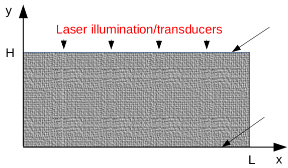
Figure 1: The geometry of the sample.

The propagation of the optical wave in the sample is modeled by the following diffusion equation

(5) $$\left\{\begin{array}[]{llllccc}-\nabla\cdot D(y)\nabla u({\bf x})+\mu_{a}(y)u({\bf x})=0&{\bf x}\in\Omega,\\ u({\bf x})=g({\bf x})&{\bf x}\in\Gamma_{m},\\ u({\bf x})=0&{\bf x}\in\Gamma_{0},\\ u(0,y)={u(L,y)}&y\in(0,H),\end{array}\right.$$

where $g$ is the laser illumination, $D$ and $\mu_{a}$ are respectively the diffusion and absorption coefficients. The part of the boundaries $\Gamma_{j}$ are given by

$$\Gamma_{m}\;=\;(0,L)\times\{y=H\}, \Gamma_{0}\;=\;(0,L)\times\{y=0\},$$

and $\partial_{\nu}$ is the derivative along $\nu$, the unit normal vector pointing outward of $\Omega$. We note that $\nu$ is everywhere defined except at the vertices of $\Omega$ and we denote by $\Gamma_{p}$ the complementary of $\overline{\Gamma_{0}}\cup\overline{\Gamma_{m}}$ in $\partial\Omega$.

We follow the approach taken in several papers [14, 15, 17] and consider two laser illuminations $g_{j},j=1,2$. Denote $u_{j},j=1,2,$ the corresponding laser intensities.

Let

$$V\,:=\,\{v\in H^{1}(\Omega);v(0,y)=v(L,y),\;y\in(0,H);u=0\,\textrm{ on }\Gamma_{0}\}.$$

We further assume that $g\in V_{\Gamma_{m}}$, where

$$V_{\Gamma_{m}}\,:=\,\{v|_{\Gamma_{m}}\in H^{1}(\Omega);v(0,y)=v(L,y),\;y\in(0,H);u=0\,\textrm{ on }\Gamma_{0}\}.$$

Then, there exists a unique solution $u\in V$ satisfying the system (5). The proof uses techniques developed in [23]. The first step is to show that the set

$$V_{0}\,:=\,\{v\in H^{1}(\Omega);v(0,y)=v(L,y),\;y\in(0,H);u=0\,\textrm{ on }\Gamma_{0}\cup\Gamma_{m}\},$$

is a closed sub space of $H^{1}(\Omega)$, using a specific trace theorem for regular curvilinear polygons (Theorem 1.5.2.8, page 50 in [23]). Then, applying the classical Lax-Milligram for elliptic operators in Lipschitz domain gives the existence and uniqueness of solution to the system (5).

Remark 2.1.

Using an explicit characterization of the trace theorem obtained in [23] one can derive the optimal local regularity for $g\in H^{\frac{1}{2}}(\Gamma_{m})$ that guarantees the existence and uniqueness of solutions to the system (5) (see also [9]).

For simplicity, we will further consider $g_{j}=\varphi_{k_{j}},j=1,2$, where $k_{1}<k_{2}$, and $\varphi_{k}(x),k\in\mathbb{N},$ is the Fourier orthonormal basis of $L^{2}(0,L)$ satisfying $-\varphi_{k}^{\prime\prime}(y)=\lambda_{k}^{2}\varphi_{k}(y)$, with $\lambda_{k}=\frac{2k\pi}{L},k\in\mathbb{Z}$. Direct calculation gives $\varphi_{k}(x)=\frac{1}{\sqrt{L}}e^{i\lambda_{k}x},k\in\mathbb{Z}$.

We assume that point-like ultrasound transducers, located on an observation surface $\Gamma_{m}$, are used to detect the values of the pressure $p({\bf x},t)$, where ${\bf x}\in\Gamma_{m}$ is a detector location and $t\geq 0$ is the time of the observation. We also assume that the speed of sound in the sample occupying $\Omega=(0,L)\times(0,H)$, is a smooth function and depends only on the vertical variable $y$, that is, $c=c(y)>0$. Then, the following model is known to describe correctly the propagating pressure wave $p({\bf x},t)$ generated by the photoacoustic effect

(11) $$\left\{\begin{array}[]{llllccc}\partial_{tt}p({\bf x},t)=c^{2}(y)\Delta p({\bf x},t)&{\bf x}\in\Omega,t\geq 0,\\ \partial_{\nu}p({\bf x},t)+\beta\partial_{t}p({\bf x},t)=0&{\bf x}\in\Gamma_{m},t\geq 0,\\ p({\bf x},t)=0&{\bf x}\in\Gamma_{0},t\geq 0,\\ p((0,y),t)=p((L,y),t)&y\in(0,H),t\geq 0,\\ p({\bf x},0)=f_{0}({\bf x}),\;\partial_{t}p({\bf x},0)=f_{1}({\bf x}),&{\bf x}\in\Omega,\end{array}\right.$$

Here $\beta>0$ is the damping coefficient, and $f_{j}({\bf x}),j=0,1,$ are the initial values of the acoustic pressure, which one needs to find in order to determine the optical parameters of the sample.

Remark 2.2.

Notice that in most existing works in photoacoustic imaging the initial state $f_{0}({\bf x})$ is given by $\mu_{a}({\bf x})u({\bf x})$, and is assumed to be compactly supported inside $\Omega$, while the initial speed $f_{1}({\bf x})$ is zero everywhere [29, 39, 43]. The compactly support assumption on $f_{0}({\bf x})$ simplifies the analysis of the inverse source initial-to-boundary problem and is necessary for almost all the existing uniqueness and stability results [10, 11, 27, 47]. Meanwhile the assumption is clearly in contradiction with the fact that $f_{0}({\bf x})$ coincides with $\mu_{a}({\bf x})u({\bf x})$ everywhere. We will show in section 4 that $\mu_{a}({\bf x})u({\bf x})$ is not only not compactly supported, it is also exponentially concentrated around the part of the boundary $\Gamma_{m}$ where we applied the laser illumination. In our model the initial speed $\partial_{t}p({\bf x},0)=f_{1}({\bf x})$ can be considered as the correction of the photoacoustic effect generated by the heat at $\Gamma_{m}$.

The following stability estimates are the main results of the paper, obtained by combining stability estimates from the acoustic and optical inversions.

Theorem 2.1.

Let $(D,\mu_{a})$,  $(\widetilde{D},\widetilde{\mu}_{a})$ in $\mathcal{O}_{M}$, and $k_{i},\,i=1,2$ be two distinct integers. Let $c(y)\in W^{1,\infty}(0,{H})$ with $0<c_{m}\leq c^{-2}(y)$ and set $\theta=\sqrt{\|c^{-2}\|_{L^{\infty}}}$. Denote $u_{k_{i}},\,i=1,2$ and $\widetilde{u}_{k_{i}},\,i=1,2$ the solutions to the system (24) for $g_{i}=\varphi_{k_{i}},i=1,2$, with coefficients $(D,\mu_{a})$ and $(\widetilde{D},\widetilde{\mu}_{a})$ respectively. Assume that $D(H)=\widetilde{D}(H)$, $D^{\prime}(H)=\widetilde{D}^{\prime}(H)$, $\mu_{a}^{\prime}(H)=\widetilde{\mu}_{a}^{\prime}(H),\,$ $k_{1}<k_{2}$, and $k_{1}$ is large enough.

Then, for $T>2\theta H$, there exists a constant $C>0$ that only depends on $\mu_{0},D_{0},k_{1},k_{2},M,L,$ and $H,$ such that the following stability estimates hold.

$$\|\underline{u}_{m}^{2}(\mu_{a}-\widetilde{\mu}_{a})\|_{C^{0}}\leq$$

$$C\left(\sum_{i=1}^{2}\int_{0}^{T}\left(\frac{C_{M}}{T-2\theta H}+\beta\right)\|\partial_{t}p_{i}-\partial_{t}\widetilde{p}_{i}\|^{2}_{L^{2}(\Gamma_{m})}+\|\partial_{x}p_{i}-\partial_{x}\widetilde{p}_{i}\|^{2}_{L^{2}(\Gamma_{m})}dt\right)^{\frac{1}{4}},$$

and

$$\|\underline{u}_{m}^{2}(D-\widetilde{D})\|_{C^{0}}\leq$$

$$C\left(\sum_{i=1}^{2}\int_{0}^{T}\left(\frac{C_{M}}{T-2\theta H}+\beta\right)\|\partial_{t}p_{i}-\partial_{t}\widetilde{p}_{i}\|^{2}_{L^{2}(\Gamma_{m})}+\|\partial_{x}p_{i}-\partial_{x}\widetilde{p}_{i}\|^{2}_{L^{2}(\Gamma_{m})}dt\right)^{\frac{1}{4}},$$

where

$$C_{M}=He^{\int_{0}^{H}c^{2}(s)|\partial_{y}(c^{-2}(s))|ds}(c^{-2}(H)+\beta^{2}),$$

$$\underline{u}_{m}(y)=\frac{D^{\frac{1}{2}}(H)}{D^{\frac{1}{2}}(y)}\frac{\sinh(\kappa_{m}^{\frac{1}{2}}y)}{\sinh(\kappa_{m}^{\frac{1}{2}}H)},\;\kappa_{m}=\min_{0\leq y\leq H}\left(\frac{(D^{\frac{1}{2}})^{\prime\prime}}{D^{\frac{1}{2}}}+\frac{\mu_{a}}{D}+\lambda_{k}^{2}\right).$$

Since the function $\underline{u}_{m}(y)$ is exponentially decreasing between the value $1$ on $\Gamma_{m}$ to the value $0$ on $\Gamma_{0}$, the stability estimates in Theorem 2.1 shows that the resolution deteriorate exponentially in the depth direction far from $\Gamma_{m}$.

3 The acoustic inversion

The data obtained by the point detectors located on the surface $\Gamma_{m}$ are represented by the function

$$p({\bf x},t)=d({\bf x},t)\qquad{\bf x}\in\Gamma_{m},\;t\geq 0.$$

Thus, the first inversion in photoacoustic imaging is to find, using the data $d({\bf x},t)$ measured by transducers, the initial value $f_{0}({\bf x})$ at $t=0$ of the solution $p({\bf x},t)$ of (11). We will also recover the initial speed $f_{1}({\bf x})$ inside $\Omega$, but we will not use it in the second inversion.

We first focus on the direct problem and prove existence and uniqueness of the acoustic problem (11). Denote by $L^{2}_{c}(\Omega)$ the Sobolev space of square integrable functions with weight $\frac{1}{c^{2}(y)}$. Since the speed $c^{2}$ is lower and upper bounded, the norm corresponding to this weight is equivalent to the classical norm of $L^{2}(\Omega)$. Let

$$V=\{p\in H^{1}(\Omega);\;p(0,y)=p(L,y),\;y\in(0,H);p=0\;\textrm{on}\;\Gamma_{0}\},$$

and consider in $V\times L^{2}_{c}(\Omega)$ the unbounded linear operator $A$ defined by

$$A(p,q)=(q,c^{2}\Delta p),\;D(A)=\{(p,q)\in V\times V;\;\Delta p\in L^{2}(\Omega);\;\partial_{\nu}p+\beta q=0\;\textrm{on}\;\Gamma_{m}\}.$$

We have the following existence and uniqueness result.

Proposition 3.1.

For $(f_{0},f_{1})\in D(A)$, the problem (11) has a unique solution $p(x,t)$ satisfying

$$(p,\partial_{t}p)\in C\left([0,+\infty),D(A)\right)\cap C^{1}\left([0,+\infty),V\times L^{2}_{c}(\Omega)\right).$$

Proof.

There are various methods for proving well-posedness of evolution problems: variational methods, the Laplace transform method and the semi-group method. Here, we will consider the semi-group method [45], and prove that the operator $A$ is m-dissipative on the Hilbert space $V\times L^{2}_{c}(\Omega)$.

Denote by $\langle\cdot,\cdot\rangle$ the scalar product in $V\times L^{2}_{c}(\Omega)$, that is, for $(p_{i},q_{i})\in V\times L^{2}_{c}(\Omega)$ with $i=1,2$,

$$\langle(p_{1},q_{1}),(p_{2},q_{2})\rangle = \int_{\Omega}\nabla p_{1}\nabla\overline{p}_{2}d{\bf x}+\int_{\Omega}q_{1}\overline{q}_{2}\frac{d{\bf x}}{c^{2}}.$$

Now let $(p,q)\in D(A)$. We have

$$\langle A(p,q),(p,q)\rangle = \int_{\Omega}\nabla q\nabla\overline{p}d{\bf x}+\int_{\Omega}\Delta p\overline{q}d{\bf x}.$$

Since $\Delta p\in L^{2}(\Omega)$ and $\partial_{\nu}p+\beta q=0\;\textrm{on}\;\Gamma_{m}$, applying Green formula leads to

$$\langle A(p,q),(p,q)\rangle = \int_{\Omega}\nabla q\nabla\overline{p}d{\bf x}-\int_{\Omega}\nabla\overline{q}\nabla pd{\bf x}-\beta\int_{\Gamma_{m}}|q|^{2}d\sigma({\bf x}).$$

Consequently

$$\Re(\langle A(p,q),(p,q)\rangle) = -\beta\int_{\Gamma_{m}}|q|^{2}d\sigma({\bf x}).$$

Therefore the operator $A$ is dissipative. The fact that $0$ is in the resolvent of $A$ is straightforward. Then $A$ is m-dissipative and hence, it is the generator of a strongly continuous semigroup of contractions [45]. Consequently, for $(f_{0},f_{1})\in D(A)$ there exists a unique strong solution to the problem (11). ∎

Now, back to the inverse problem of reconstructing the initial data $(f_{0},f_{1})$. We further assume that the initial data is generated by a finite number of Fourier modes, that is

(12) $$f_{j}(x,y) = \sum_{|k|\leq N}f_{jk}(y)\varphi_{k}(x)\qquad(x,y)\in\Omega\qquad j=0,1,$$

with $N$ being a fixed positive integer.

As it was already remarked in many works, this linear initial-to-boundary inverse problem is strongly related to boundary observability of the source from the set $\Gamma_{m}$ (see for instance [33, 43, 45, 48]). We will emphasize on the links between our findings and known results in this context later. Here we will use a different approach taking advantage of the fact that the wave speed $c(y)$ only depends in the vertical variable $y$.

Since $p({\bf x})$ is $L$-periodic in the $y$ variable, it has the following discrete Fourier decomposition

$$p(x,y) = \sum_{|k|\leq N}p_{k}(y,t)\varphi_{k}(x)\qquad(x,y)\in\Omega.$$

One can check that $p_{k}(y,t)\varphi_{k}(x)$ is exactly the solution to the problem (11) with initial data $(f_{0k}(y)\varphi_{k}(x),f_{1k}(y)\varphi_{k}(x))$. Precisely, if $\lambda_{k}=\frac{2k\pi}{L}$, the functions $p_{k}(y,t)$ satisfy the following one dimensional wave equation

(17) $$\left\{\begin{array}[]{llllccc}\frac{1}{c^{2}(y)}\partial_{tt}p(y,t)=\partial_{yy}p(y,t)-\lambda_{k}^{2}p(y,t),&y\in(0,H),t\geq 0,\\ \partial_{y}p(H,t)+\beta\partial_{t}p(H,t)=0&t\geq 0,\\ p(0,t)=0&t\geq 0,\\ p(y,0)=f_{0k}(y),\;\partial_{t}p(y,0)=f_{1k}(y),&y\in(0,H),\end{array}\right.$$

Next, we will focus on the boundary observability problem of the initial data $f_{k}$ at the extremity $y=H$. Taking advantage of the fact that the equation is one dimensional we will derive a boundary observability inequality with a sharp constant. Define $E(t)$ the total energy of the system (17) by

(18) $$E(t) = \int_{0}^{H}\left(c^{-2}(y)|\partial_{t}p(y,t)|^{2}+|\partial_{y}p(y,t)|^{2}+\lambda_{k}^{2}|p(y,t)|^{2}\right)dy.$$

Multiplying the first equation in the system (17) by $\partial_{t}p(y,t)$ and integrating over $(0,H)$ leads to

(19) $$E^{\prime}(t)=-\beta|\partial_{t}p(H,t)|^{2}\qquad\textrm{for}\quad t\geq 0.$$

Consequently, $E(t)$ is a non-increasing function, and the decay is clearly related to the magnitude of the dissipation on the boundary $\Gamma_{m}$.

It is well know that the system (17) has a unique solution. Here we establish an estimate of the continuity constant.

Proposition 3.2.

Assume that $c(y)\in W^{1,\infty}(0,{H})$ with $0<c_{m}\leq c^{-2}(y)$. Then, for any $T>0$ we have

$$\beta^{2}\int_{0}^{T}|\partial_{t}p_{k}(H,t)|^{2}dt\leq((C_{m}^{1}+C_{m}^{2}\lambda_{k})T+C_{m}^{3})E_{k}(0),$$

for $k\in\mathbb{N}$, where

$$E_{k}(0)=\int_{0}^{H}\left(c^{-2}(y)|f_{1k}(y)|^{2}+|f_{0k}^{\prime}(y)|^{2}+\lambda_{k}^{2}|f_{0k}(y)|^{2}\right)dy,$$

$$C_{m}^{1}=(1+Hc^{-2}(H))^{-1}\left(1+(1+\frac{H}{c_{m}})\|c^{-2}\|_{W^{1,\infty}}\right),$$

$$C_{m}^{3}=(1+Hc^{-2}(H))^{-1}\left(1+2H\|c^{-2}\|_{L^{\infty}}^{1/2}\right),$$

$$C_{m}^{2}=H(1+Hc^{-2}(H))^{-1}.$$

Proposition 3.3.

Assume that $c(y)\in W^{1,\infty}(0,{H})$ with $0<c_{m}\leq c^{-2}(y)$. Let $\theta=\sqrt{\|c^{-2}\|_{L^{\infty}}}$ and $T>2\theta H$. Then the following inequalities hold

$$\lambda_{k}^{2}\int_{0}^{H}|f_{0k}(y)|^{2}dy\leq\left(\frac{C_{M}}{T-2\theta H}+\beta\right)\int_{0}^{T}|\partial_{t}p_{k}(H,t)|^{2}dt$$

$$+\lambda_{k}^{2}\int_{0}^{T}|p_{k}(H,t)|^{2}dt,$$

for $k\in\mathbb{N}^{*}$,

$$\int_{0}^{H}c^{-2}(y)|f_{1k}(y)|^{2}+|f_{0k}^{\prime}(y)|^{2}dy\leq\left(\frac{C_{M}}{T-2\theta H}+\beta\right)\int_{0}^{T}|\partial_{t}p_{k}(H,t)|^{2}dt$$

$$+\lambda_{k}^{2}\int_{0}^{T}|p_{k}(H,t)|^{2}dt,$$

for $k\in\mathbb{N}$, with

$$C_{M}=He^{\int_{0}^{H}c^{2}(s)|\partial_{y}(c^{-2}(s))|ds}(c^{-2}(H)+\beta^{2}).$$

The proofs of these results are given in the Appendix. The main result of this section is the following.

Theorem 3.1.

Assume that $c(y)\in W^{1,\infty}(0,1)$ with $0<c_{m}\leq c^{-2}(y)$, and $f_{0},f_{1}$ have a finite Fourier expansion (12). Let $\theta=\sqrt{\|c^{-2}\|_{L^{\infty}}}$ and $T>2\theta H$. Then

$$\int_{\Omega}|\nabla f_{0}({\bf x})|^{2}d{\bf x}\leq\left(\frac{C_{M}}{T-2\theta H}+\beta\right)\int_{0}^{T}\|\partial_{t}p({\bf x},t)\|^{2}_{L^{2}(\Gamma_{m})}dt$$

$$+\int_{0}^{T}\|\partial_{x}p({\bf x},t)\|^{2}_{L^{2}(\Gamma_{m})}dt,$$

and

$$\int_{\Omega}c^{-2}(y)|f_{1}({\bf x})|^{2}d{\bf x}\leq\left(\frac{C_{M}}{T-2\theta H}+\beta\right)\int_{0}^{T}\|\partial_{t}p_{k}({\bf x},t)\|^{2}_{L^{2}(\Gamma_{m})}dt$$

$$+\int_{0}^{T}\|\partial_{x}p({\bf x},t)\|^{2}_{L^{2}(\Gamma_{m})}dt,$$

with

$$C_{M}=He^{\int_{0}^{H}c^{2}(s)|\partial_{y}(c^{-2}(s))|ds}(c^{-2}(H)+\beta^{2}).$$

Proof.

The estimates are direct consequences of Proposition 3.2 and Proposition 3.3. The fact that the Fourier series of $p({\bf x},t)$ has a finite number of terms justifies the regularity of the solution $p({\bf x},t)$, and allow interchanging the order between the Fourier series and the integral over $(0,T)$. ∎

Using microlocal analysis techniques it is known that the boundary observability in a rectangle holds if the set of boundary observation necessarily contains at least two adjacent sides [18, 20]. Then, we expect that the the Lipschitz stability estimate in Theorem 3.1 will deteriorate when the number of modes $N$ becomes larger. In fact the series on the right side does not converge because $\partial_{x}p({\bf x},t)$ does not belong in general to $L^{2}(\Gamma_{m}\times(0,T))$. We here provide a hölder stability estimate that corresponds to the boundary observability on only one side of the rectangle.

Theorem 3.2.

Assume that $c(y)\in W^{1,\infty}(0,1)$ with $0<c_{m}\leq c^{-2}(y)$, and $(f_{0},f_{1})\in H^{2}(\Omega)\times H^{1}(\Omega)$ satisfying $\|f_{0}\|_{H^{1}},\|f_{1}\|_{H^{2}}\leq\widetilde{M}$. Let $\theta=\sqrt{\|c^{-2}\|_{L^{\infty}}}$ and $T>2\theta H$. Then

$$\int_{\Omega}|\nabla f_{0}({\bf x})|^{2}d{\bf x}\leq\left(\frac{C_{M}}{T-2\theta H}+\beta\right)\int_{0}^{T}\|\partial_{t}p({\bf x},t)\|^{2}_{L^{2}(\Gamma_{m})}dt$$

$$+C_{\widetilde{M}}\left(\int_{0}^{T}\|p({\bf x},t)\|^{2}_{H^{\frac{1}{2}}(\Gamma_{m})}dt\right)^{\frac{2}{3}},$$

and

$$\int_{\Omega}c^{-2}(y)|f_{1}({\bf x})|^{2}d{\bf x}\leq\left(\frac{C_{M}}{T-2\theta H}+\beta\right)\int_{0}^{T}\|\partial_{t}p_{k}({\bf x},t)\|^{2}_{L^{2}(\Gamma_{m})}dt$$

$$+C_{\widetilde{M}}\theta^{\frac{2}{3}}\left(\int_{0}^{T}\|p({\bf x},t)\|^{2}_{H^{\frac{1}{2}}(\Gamma_{m})}dt\right)^{\frac{2}{3}},$$

with

$$C_{M}=He^{\int_{0}^{H}c^{2}(s)|\partial_{y}(c^{-2}(s))|ds}(c^{-2}(H)+\beta^{2}),\;C_{\widetilde{M}}=2\widetilde{M}^{\frac{2}{3}}.$$

Proof.

The proof is again based on the results of Proposition 3.3. We first deduce from Proposition 3.1 that $\partial_{t}p({\bf x},t)\in L^{2}(\Gamma_{m})$. Now, define

$$f_{j}^{N}({\bf x}) = \sum_{|k|\leq N}f_{jk}(y)\varphi_{k}(x)\qquad{\bf x}\in\Omega\qquad j=0,1,$$

with $f_{jk}(y)$ are the Fourier coefficients of $f_{j}({\bf x})$, and $N$ being a large positive integer.

Consequently

(20) $$\int_{\Omega}|\nabla f_{0}({\bf x})|^{2}d{\bf x}\leq\int_{\Omega}|\nabla f_{0}^{N}({\bf x})|^{2}d{\bf x}+\frac{\widetilde{M}^{2}}{\lambda_{N+1}^{2}},$$

(21) $$\int_{\Omega}c^{-2}(y)|f_{1}({\bf x})|^{2}d{\bf x}\leq\int_{\Omega}c^{-2}(y)|f_{1}^{N}({\bf x})|^{2}d{\bf x}+\frac{\theta^{2}\widetilde{M}^{2}}{\lambda_{N+1}^{2}},$$

for $N$ large. Applying now Proposition 3.3 to $(f_{0}^{N},f_{1}^{N})$, gives

$$\int_{\Omega}|\nabla f_{0}({\bf x})|^{2}d{\bf x}\leq\left(\frac{C_{M}}{T-2\theta H}+\beta\right)\int_{0}^{T}\|\partial_{t}p({\bf x},t)\|^{2}_{L^{2}(\Gamma_{m})}dt$$

$$+\lambda_{N}\int_{0}^{T}\|p({\bf x},t)\|^{2}_{H^{\frac{1}{2}}(\Gamma_{m})}dt+\frac{\widetilde{M}^{2}}{\lambda_{N+1}^{2}},$$

$$\int_{\Omega}c^{-2}(y)|f_{1}({\bf x})|^{2}d{\bf x}\leq\left(\frac{C_{M}}{T-2\theta H}+\beta\right)\int_{0}^{T}\|\partial_{t}p({\bf x},t)\|^{2}_{L^{2}(\Gamma_{m})}dt$$

$$+\lambda_{N}\int_{0}^{T}\|p({\bf x},t)\|^{2}_{H^{\frac{1}{2}}(\Gamma_{m})}dt+\frac{\theta^{2}\widetilde{M}^{2}}{\lambda_{N+1}^{2}}.$$

By minimizing the right hand terms with respect to the value of $\lambda_{N}$, we obtain the desired results.

∎

4 The optical inversion

Once the initial pressure $f_{0}({\bf x})$, generated by the optical wave has been reconstructed, a second step consists of determining the optical properties in the sample. Although this second step has not been well studied in biomedical literature due its complexity, it is of importance in applications. In fact the optical parameters are very sensitive to the tissue condition and their values for healthy and unhealthy tissues are extremely different.

The second inversion is to determine the coefficients $(D(y),\mu_{a}(y))$ from the initial pressures recovered in the first inversion, that is, ${h}_{j}({\bf x})=\mu_{a}(y)u_{j}({\bf x}),\;{\bf x}\in\Omega,\;j=1,2$.

For simplicity, we will consider $g_{j}({\bf x})=\varphi_{k_{j}}(x),\;j=1,2$ with $k_{1}$ and $k_{2}$ are two distinct Fourier eigenvalues that are large enough. We specify how large they should be later in the analysis.

The main result of this section is the following.

Theorem 4.1.

Let $(D,\mu_{a})$,  $(\widetilde{D},\widetilde{\mu}_{a})$ in $\mathcal{O}_{M}$, and $k_{i},\,i=1,2$ be two distinct integers. Denote $u_{k_{i}},\,i=1,2$ and $\widetilde{u}_{k_{i}},\,i=1,2$ the solutions to the system (24) for $g_{i}=\varphi_{k_{i}},i=1,2$, with coefficients $(D,\mu_{a})$ and $(\widetilde{D},\widetilde{\mu}_{a})$ respectively. Assume that $D(H)=\widetilde{D}(H)$, $D^{\prime}(H)=\widetilde{D}^{\prime}(H)$, $\mu_{a}^{\prime}(H)=\widetilde{\mu}_{a}^{\prime}(H),\,$ $k_{1}<k_{2}$, and $k_{1}$ is large enough. Then, there exists a constant $C>0$ that only depends on $(\mu_{0},D_{0},k_{1},k_{2},M,L,H)$, such that the following stability estimates hold.

$$\|\underline{u}_{m}^{2}(D-\widetilde{D})\|_{C^{0}}\leq C\left(\|h_{1}-\widetilde{h}_{1}\|_{C^{1}}+\|h_{2}-\widetilde{h}_{2}\|_{C^{1}}\right),$$

$$\|\underline{u}_{m}^{2}(\mu_{a}-\widetilde{\mu}_{a})\|_{C^{0}}\leq C\left(\|h_{1}-\widetilde{h}_{1}\|_{C^{1}}+\|h_{2}-\widetilde{h}_{2}\|_{C^{1}}\right).$$

Classical elliptic operator theory implies the following result for the direct problem [35].

Proposition 4.1.

Assume $(D,\mu_{a})$ be in $\mathcal{O}_{M}$ and $g\in V_{\Gamma_{m}}$. Then, there exists a unique solution $u\in V$ to the system (5). It verifies

$$\|u\|_{H^{1}(\Omega)}\leq C_{0}\|g\|_{H^{\frac{1}{2}}(\Gamma_{m})}^{2},$$

where $C_{0}=C_{0}(\mu_{0},D_{0},M,L,H)>0$.

For $g({\bf x})=\varphi_{k}(x)$, the unique solution $u$ has the following decomposition

$$u({\bf x}) = u_{k}(y)\varphi_{k}(x)\qquad{\bf x}\in\Omega,$$

where $u_{k}(y)$ satisfies the following one dimensional elliptic equation

(24) $$\left\{\begin{array}[]{llllccc}-\left(D(y)u^{\prime}(y)\right)^{\prime}+(\mu_{a}(y)+\lambda_{k}^{2}D(y))u(y)=0&y\in(0,H),\\ u(H)=1,\;\;u(0)=0,&\end{array}\right.$$

Next we will derive some useful properties of the solution to the system  (24).

Lemma 4.1.

Let $u(y)$ be the unique solution to the system  (24). Then $u(y)\in C^{2}([0,H])$ and there exists a constant $b=b(\mu_{0},D_{0},M,L,H)>0$ such that $\|u\|_{C^{2}}\leq b$ for all $(D,\mu_{a})\in\mathcal{O}_{M}$. In addition the following inequalities hold for $k$ large enough.

$$\underline{u}_{m}(y)\leq u(y)\leq\overline{u}_{M}(y),$$

for $0\leq y\leq H$, where

$$\underline{u}_{m}(y)=\frac{D^{\frac{1}{2}}(H)}{D^{\frac{1}{2}}(y)}\frac{\sinh(\kappa_{m}^{\frac{1}{2}}y)}{\sinh(\kappa_{m}^{\frac{1}{2}}H)},\quad\overline{u}_{M}(y)=\frac{D^{\frac{1}{2}}(H)}{D^{\frac{1}{2}}(y)}\frac{\sinh(\kappa_{M}^{\frac{1}{2}}y)}{\sinh(\kappa_{M}^{\frac{1}{2}}H)},$$

$$\kappa_{m}=\min_{0\leq y\leq H}\left(\frac{(D^{\frac{1}{2}})^{\prime\prime}}{D^{\frac{1}{2}}}+\frac{\mu_{a}}{D}+\lambda_{k}^{2}\right),\quad\kappa_{M}=\max_{0\leq y\leq H}\left(\frac{(D^{\frac{1}{2}})^{\prime\prime}}{D^{\frac{1}{2}}}+\frac{\mu_{a}}{D}+\lambda_{k}^{2}\right).$$

Proof.

We first make the Liouville change of variables and introduce the function

$$v(y)=\frac{D^{\frac{1}{2}}(y)}{D^{\frac{1}{2}}(H)}u(y).$$

Forward calculations show that $v(y)$ is the unique solution to the following system.

(27) $$\left\{\begin{array}[]{llllccc}-v^{\prime\prime}(y)+\kappa(y)v(y)=0&y\in(0,H),\\ v(H)=1,\;\;v(0)=0,&\end{array}\right.$$

where

$$\kappa(y)=\frac{(\sqrt{D})^{\prime\prime}}{\sqrt{D}}+\frac{\mu_{a}}{D}+\lambda_{k}^{2}.$$

Assume now that $k$ is large enough such that $\kappa_{m}>0$, and let $\underline{v}_{m}(y)$ and $\overline{v}_{M}(y)$ be the solutions to the system (27) when we replace $\kappa(y)$ by respectively the constants $\kappa_{m}$ and $\kappa_{M}$. They are explicitly given by

$$\underline{v}_{m}(y) = \frac{\sinh(\sqrt{\kappa_{m}}y)}{\sinh(\sqrt{\kappa_{m}}H)},$$

$$\overline{v}_{M}(y) = \frac{\sinh(\sqrt{\kappa_{M}}y)}{\sinh(\sqrt{\kappa_{M}}H)}.$$

The maximum principle [35] implies that $0<v(y),\underline{v}_{m}(y),\overline{v}_{M}(y)<1$ for $0<y<H$.

By applying again the maximum principle on the differences $v-\underline{v}_{m}$ and $v-\overline{v}_{M}$ we deduce that $\underline{v}_{m}(y)<v(y)<\overline{v}_{M}(y)$ for $0\leq y\leq H$, which leads to the desired lower and upper bounds.

We deduce from the regularity of the coefficients $D$ and $\mu_{a}$ and the classical elliptic regularity [35] that $u\in H^{3}(0,H)$. Moreover there exist a constant $b>$ that only depends on $(\mu_{0},D_{0},M,L,H)$ such that

(28) $$\|u\|_{H^{3}}\leq b.$$

Consequently the uniform $C^{2}$ bound of $u$ can be obtained using the continuous Sobolev embedding of $H^{3}(0,H)$ into $C^{2}([0,H])$ [1].

∎

Lemma 4.2.

Let $(D,\mu_{a})\in\mathcal{O}_{M}$, and $u(y)$ be the unique solution to the system (24). Then, for $k$ large enough there exists a constant $\varrho=\varrho(D_{0},\mu_{0},M,k)>0$ such that

$$u^{\prime}(y)\geq\varrho,$$

for $0\leq y\leq H$.

Proof.

Since $0$ is the global minimum of $u(y)$, we have $u^{\prime}(0)>0$. Moreover for $k$ large enough, Lemma 4.1 implies that

$$u(y)\geq\frac{\sqrt{D(H)}}{\sqrt{D(y)}}\frac{\sinh(\sqrt{\kappa_{m}}y)}{\sinh(\sqrt{\kappa_{m}}H)},$$

for all $y\in[0,H]$. Therefore

$$u^{\prime}(0)\geq\frac{\sqrt{D(H)}}{\sqrt{\|D\|_{L^{\infty}}}}\frac{\sqrt{\kappa_{m}}}{\sinh(\sqrt{\kappa_{m}}H)}$$

Now integrating equation (24) over $(0,y)$ we obtain

$$D(y)u^{\prime}(y)=D(0)u^{\prime}(0)+\int_{0}^{y}(\mu_{a}(s)+\lambda_{k}^{2}D(s))u(s)ds$$

$$D(y)u^{\prime}(y)\geq D(0)u^{\prime}(0)+\int_{0}^{y}(\mu_{a}(s)+\lambda_{k}^{2}D(s))\frac{\sqrt{D(H)}}{\sqrt{D(s)}}\frac{\sinh(\sqrt{\kappa_{m}}s)}{\sinh(\sqrt{\kappa_{m}}H)}ds$$

$$\geq\frac{\sqrt{D(H)}}{\sqrt{\|D\|_{L^{\infty}}}}\frac{\sqrt{\kappa_{m}}D_{0}}{\sinh(\sqrt{\kappa_{m}}H)}+(\mu_{0}+\lambda_{k}^{2}D_{0})\frac{\sqrt{D(H)}}{\sqrt{\|D\|_{L^{\infty}}}}\frac{\cosh(\sqrt{\kappa_{m}}y)-1}{\sinh(\sqrt{\kappa_{m}}H)}.$$

Taking into account the explicit expression of $\kappa_{m}$ finishes the proof. ∎

Since the illumination are chosen to coincide with the Fourier basis functions $\varphi_{k_{j}},\,j=1,2$, the data ${\bf h}_{j}({\bf x}),\,j=1,2$, can be rewritten as ${\bf h}_{j}({\bf x})=h_{j}(y)\varphi_{k_{j}}(x),\,j=1,2$, where $h_{j}(y)=\mu_{a}(y)u_{k_{j}}(y)$.

Therefore the optical inversion is reduced to the problem of identifying the optical pair $(D,\mu_{a})$ from the knowledge of the pair $(h_{1}(y),h_{2}(y))$ over $(0,H)$.

Let $(D,\mu_{a})$,  $(\widetilde{D},\widetilde{\mu}_{a})$ be two different pairs in $\mathcal{O}_{M}$, and denote $u_{k}$ and $\widetilde{u}_{k}$ the solutions to the system (24), with coefficients $(D,\mu_{a})$ and $(\widetilde{D},\widetilde{\mu}_{a})$ respectively.

We deduce from Lemma 4.1 that $\frac{1}{u_{k}}$ and $\frac{1}{\widetilde{u}_{k}}$ lie in $L^{p}(0,H)$ for $0<p<1$. Unfortunately for or $0<p<1$ the usual $\|\cdot\|_{L^{p}}$ is not anymore a norm on the vector space $L^{p}(0,H)$ because it does not satisfy the triangle inequality (see for instance [1]). In contrast with triangle inequality Hölder inequality holds for $0<p<1$, and we have

(29) $$\|\frac{v}{u_{k}}\|_{L^{r}}\leq\|\frac{1}{u_{k}}\|_{L^{p}}\|v\|_{L^{q}},$$

for all $v\in L^{q}(0,H)$ with $\frac{1}{r}=\frac{1}{p}+\frac{1}{q}$.

Consequently $h=\frac{h_{2}}{h_{1}}=\frac{u_{k_{2}}}{u_{k_{1}}}$ can be considered as a distribution that coincides with a $C^{2}$ function over $(0,H)$. A forward calculation shows that $h$ satisfies the equation

(30) $$-\left(Du_{k_{1}}^{2}h^{\prime}\right)^{\prime}+Du_{k_{1}}^{2}h(\lambda_{2}^{2}-\lambda_{1}^{2})=0,$$

over $(0,H)$.

Since $u_{k_{j}},\,j=1,2$ are in $C^{2}([0,H])$, an asymptotic analysis of $D(y)u_{k_{1}}^{2}(y)h^{\prime}(y)$ at $0$ and the results of Lemma 4.1, gives

$$\lim_{y\to 0}Du_{k_{1}}^{2}h^{\prime}=0.$$

Similarly, we have

$$\lim_{y\to 1}h=1.$$

Integrating the equation (30) over $(0,y)$, we get

$$D(y)u_{k_{1}}^{2}(y)h^{\prime}(y)=(\lambda_{2}^{2}-\lambda_{1}^{2})\int_{0}^{y}D(s)u_{k_{1}}(s)u_{k_{2}}(s)ds.$$

Dividing both sides by $D(y)u_{k_{1}}^{2}(y)$, and using again Lemma 4.1, imply

$$h^{\prime}(y)\geq(\lambda_{2}^{2}-\lambda_{1}^{2})D^{-1}(y)\overline{u}_{M}^{-2}(y)\int_{0}^{y}D(s)\underline{u}_{m}^{2}(s)ds,$$

which leads to

(31) $$h^{\prime}(y)\geq(\lambda_{2}^{2}-\lambda_{1}^{2})\min_{y\in(0,H)}D^{-1}(y)\overline{u}_{M}^{-2}(y)\int_{0}^{y}D(s)\underline{u}_{m}^{2}(s)ds>0.$$

The right hand constant is strictly positive and only depends on $D_{0},\mu_{0},M,H,L$ and $k$.

Now back to the optical inversion. The equation (30) can be written as

$$-(Du_{k_{1}}^{2})^{\prime}h^{\prime}+\left(h(\lambda_{2}^{2}-\lambda_{1}^{2})-h^{\prime\prime}\right)Du_{k_{1}}^{2}=0,$$

over $(0,H)$. Dividing both sides by $Du_{k_{1}}^{2}h^{\prime}$, and integrating over $(0,y)$, we obtain

(32) $$D(y)u_{k_{1}}^{2}(y)=h(0)-h(y)+e^{(\lambda_{2}^{2}-\lambda_{1}^{2})\int_{0}^{y}\frac{h}{h^{\prime}}ds}.$$

This allows us to show the following result.

Lemma 4.3.

Under the assumptions of Theorem 4.1, there exists a constant $C=C(\mu_{0},D_{0},k_{1},k_{2},M,L,H)>0$ such that the following inequality holds.

$$\|Du_{k_{1}}^{2}-\widetilde{D}\widetilde{u}_{k_{1}}^{2}\|_{C^{0}}\leq C\left(\|h_{1}-\widetilde{h}_{1}\|_{C^{1}}+\|h_{2}-\widetilde{h}_{2}\|_{C^{1}}\right).$$

Proof.

Recall that the relation (32) is also valid for the pair $(\widetilde{D},\widetilde{\mu}_{a})$, that is

$$\widetilde{D}(y)\widetilde{u}_{k_{1}}^{2}(y)=\widetilde{h}(0)-\widetilde{h}(y)+e^{(\lambda_{2}^{2}-\lambda_{1}^{2})\int_{0}^{y}\frac{\widetilde{h}}{\widetilde{h}^{\prime}}ds},$$

where $\widetilde{h}=\frac{\widetilde{u}_{k_{2}}}{\widetilde{u}_{k_{1}}}$. Taking the difference between the last equation and the equation (32) we find

$$\|Du_{k_{1}}^{2}-\widetilde{D}\widetilde{u}_{k_{1}}^{2}\|_{C^{0}}\leq\|h-\widetilde{h}\|_{C^{0}}+(\lambda_{2}^{2}-\lambda_{1}^{2})H\left\|\frac{h}{h^{\prime}}-\frac{\widetilde{h}}{\widetilde{h}^{\prime}}\right\|_{C^{0}}e^{(\lambda_{2}^{2}-\lambda_{1}^{2})H\left(\left\|\frac{h}{h^{\prime}}\right\|_{C^{0}}+\left\|\frac{\widetilde{h}}{\widetilde{h}^{\prime}}\right\|_{C^{0}}\right)}.$$

We then deduce the result from Lemma 4.1 and inequality (31).

∎

Now, we are ready to prove the main stability result of this section. We remark as in [14], that $\frac{1}{u_{k_{1}}}$ is a solution to the following equation.

$$-\left(Du_{k_{1}}^{2}\frac{1}{u_{k_{1}}}^{\prime}\right)^{\prime}+\lambda_{k_{1}}^{2}Du_{k_{1}}^{2}\frac{1}{u_{k_{1}}}=h_{1}, y\in(0,H).$$

Since $\frac{1}{\widetilde{u}_{k_{1}}}$ solves the same type of equation, we obtain that $w=\frac{1}{u_{k_{1}}}-\frac{1}{\widetilde{u}_{k_{1}}}$, is the solution to the following system

(35) $$\left\{\begin{array}[]{llcc}-\left(Du_{k_{1}}^{2}w^{\prime}\right)^{\prime}+\lambda_{k_{1}}^{2}Du_{k_{1}}^{2}w=e,&y\in(0,H),\\ w(H)=0,\;w^{\prime}(H)=\frac{1}{\mu_{a}(H)}(\widetilde{h}_{1}^{\prime}(H)-h_{1}^{\prime}(H)),&yw(y)\in L^{2}(0,H),\end{array}\right.$$

where

$$e=-\left((Du_{k_{1}}^{2}-\widetilde{D}\widetilde{u}_{k_{1}}^{2})\frac{1}{\widetilde{u}_{k_{1}}}^{\prime}\right)^{\prime}+\lambda_{k_{1}}^{2}(Du_{k_{1}}^{2}-\widetilde{D}\widetilde{u}_{k_{1}}^{2})\frac{1}{\widetilde{u}_{k_{1}}}+h_{1}-\widetilde{h}_{1}.$$

We remark that to solve this system we have to deal with two main difficulties, the first is that the operator is elliptic degenerate, and the second is that the solution $w(y)$ may be unbounded at $y=0$.

Multiplying by $\mathrm{sign}(w)$, and integrating over $(s,H)$ the first equation of the system leads to

$$D(s)u_{k_{1}}^{2}(s)|w|^{\prime}(s)=$$

$$\mathrm{sign}(w)\left(\frac{D(H)}{\mu_{a}(H)}(\widetilde{h}_{1}^{\prime}(H)-h_{1}^{\prime}(H))+\int_{s}^{H}e(y)dy-\lambda_{k_{1}}^{2}\int_{s}^{H}D(y)u_{k_{1}}^{2}(y)w(y)dy\right).$$

Integrating again over $(t,H)$ gives

$$\int_{t}^{H}D(s)u_{k_{1}}^{2}(s)|w|^{\prime}(s)ds\leq$$

$$\frac{MH}{\mu_{0}}\|h_{1}-\widetilde{h}_{1}\|_{C^{1}}+\int_{0}^{H}\left|\int_{s}^{H}e(y)dy\right|ds+\lambda_{k_{1}}^{2}H\int_{0}^{H}D(y)u_{k_{1}}^{2}(y)|w|(y)dy.$$

Since $u_{k_{1}}^{\prime}>0$ over $(0,H)$ (Lemma 4.2), $u_{k_{1}}$ is increasing, and we have

$$D(t)u_{k_{1}}^{2}(t)|w|(t)\leq$$

$$\frac{MH}{\mu_{0}}\|h_{1}-\widetilde{h}_{1}\|_{C^{1}}+\int_{0}^{H}\left|\int_{s}^{H}e(y)dy\right|ds+\lambda_{k_{1}}^{2}H\int_{0}^{H}D(y)u_{k_{1}}^{2}(y)|w|(y)dy.$$

Now, we focus on the second term on the right hand side.

(36) $$\int_{0}^{H}\left|\int_{s}^{H}e(y)dy\right|ds\leq$$

$$\int_{0}^{H}|Du_{k_{1}}^{2}-\widetilde{D}\widetilde{u}_{k_{1}}^{2}|\frac{|\widetilde{u}_{k_{1}}^{\prime}|}{|\widetilde{u}_{k_{1}}^{2}|}ds+\lambda_{k_{1}}^{2}H\int_{0}^{H}|Du_{k_{1}}^{2}-\widetilde{D}\widetilde{u}_{k_{1}}^{2}|\frac{1}{|\widetilde{u}_{k_{1}}|}dy+H\|h_{1}-\widetilde{h}_{1}\|_{C^{0}}.$$

Using the estimates in Lemma 4.3, we find

(37) $$\int_{0}^{H}\left|\int_{s}^{H}e(y)dy\right|ds\leq C\left(\|h_{1}-\widetilde{h}_{1}\|_{C^{1}}+\|h_{2}-\widetilde{h}_{2}\|_{C^{1}}\right).$$

Combining inequalities (36) and (37), leads to

(38) $$D(t)u_{k_{1}}^{2}(t)|w|(t)\leq$$

$$C_{1}\left(\|h_{1}-\widetilde{h}_{1}\|_{C^{1}}+\|h_{2}-\widetilde{h}_{2}\|_{C^{1}}\right)+C_{2}\int_{t}^{H}D(y)u_{k_{1}}^{2}(y)|w|(y)dy,$$

for $0\leq t\leq H$.

Using Gronwall’s inequality we get

$$D(t)u_{k_{1}}^{2}(t)|w|(t)\leq C_{1}e^{C_{2}\int_{0}^{H}D(y)u_{k_{1}}^{2}(y)dy}\left(\|h_{1}-\widetilde{h}_{1}\|_{C^{1}}+\|h_{2}-\widetilde{h}_{2}\|_{C^{1}}\right),$$

for $0\leq t\leq H$.
Finally, we obtain the following estimate.

(39) $${u}_{k_{1}}^{2}(t)|w|(t)\leq D_{0}^{-1}C_{1}e^{C_{2}\int_{0}^{H}D(y)u_{k_{1}}^{2}(y)dy}\left(\|h_{1}-\widetilde{h}_{1}\|_{C^{1}}+\|h_{2}-\widetilde{h}_{2}\|_{C^{1}}\right),$$

The following Lemma is a direct consequence of the previous inequality.

Lemma 4.4.

Under the assumptions of Theorem 4.1, there exists a constant $C=C(\theta,\mu_{0},D_{0},k_{1},k_{2},M,L,H)>0$ such that the following inequality holds.

$$\|{u}_{k_{1}}(u_{k_{1}}-\widetilde{u}_{k_{1}})\|_{C^{0}}\leq C\left(\|h_{1}-\widetilde{h}_{1}\|_{C^{1}}+\|h_{2}-\widetilde{h}_{2}\|_{C^{1}}\right).$$

Proof.

(Theorem 4.1) Recall that $h_{1}=\mu_{a}u_{k_{1}}$ and $\widetilde{h}_{1}=\widetilde{\mu}_{a}\widetilde{u}_{k_{1}}$ over $(0,H)$.

Therefore

$$u_{k_{1}}^{2}|\mu_{a}-\widetilde{\mu}_{a}|\leq u_{k_{1}}|h_{1}-\widetilde{h}_{1}|+\widetilde{\mu}_{a}u_{k_{1}}|u_{k_{1}}-\widetilde{u}_{k_{1}}|.$$

Lemma 4.4 implies

(40) $$\|u_{k_{1}}^{2}(\mu_{a}-\widetilde{\mu}_{a})\|_{C^{0}}\leq C\left(\|h_{1}-\widetilde{h}_{1}\|_{C^{1}}+\|h_{2}-\widetilde{h}_{2}\|_{C^{1}}\right).$$

A simple calculation yields

$$u_{k_{1}}^{2}|D-\widetilde{D}|\leq\widetilde{D}|u_{k_{1}}^{2}-\widetilde{u}_{k_{1}}^{2}|+|Du_{k_{1}}^{2}-\widetilde{D}\widetilde{u}_{k_{1}}^{2}|,$$

over $(0,H)$.

Lemma 4.3 and 4.4 leads to

(41) $$\|u_{k_{1}}^{2}(D-\widetilde{D})\|_{C^{0}}\leq C\left(\|h_{1}-\widetilde{h}_{1}\|_{C^{1}}+\|h_{2}-\widetilde{h}_{2}\|_{C^{1}}\right).$$

Applying the bounds in Lemma 4.1, we obtain the wanted results. ∎

5 Proof of Theorem 2.1

The main idea here is to combine the stability results of the acoustic and optic inversions in a result that shows how the reconstruction of the optical coefficients is sensitive to the noise in the measurements of the acoustic waves.

The principal difficulty is that the vector spaces used in both stability estimates are not the same due to the difference in the techniques used to derive them. We will use interpolation inequality between Sobolev spaces to overcome this difficulty.

We deduce from the uniform bound on the solutions $u_{i},\,i=1,2$ (see for instance (28) in the proof of Lemma 4.1) that

(42) $$\|h_{i}\|_{H^{3}},\|\widetilde{h}_{i}\|_{H^{3}}\leq Mb,\quad i=1,2,$$

for all pairs $(D,\mu_{a})$and $(\widetilde{D},\mu_{a})$ in $\mathcal{O}_{M}$.

The Sobolev interpolation inequalities and embedding theorems [1] imply

$$\|h_{i}-\widetilde{h}_{i}\|_{C^{1}}\leq C\|h_{i}-\widetilde{h}_{i}\|_{H^{2}}\leq\widetilde{C}\|h_{i}-\widetilde{h}_{i}\|_{H^{1}}^{\frac{1}{2}}\|h_{i}-\widetilde{h}_{i}\|_{H^{3}}^{\frac{1}{2}},\quad i=1,2,$$

which combined with (42) gives

(43) $$\|h_{i}-\widetilde{h}_{i}\|_{C^{1}}\leq\widetilde{\widetilde{C}}\|h_{i}-\widetilde{h}_{i}\|_{H^{1}}^{\frac{1}{2}},\quad i=1,2.$$

Since the acoustic inversion is linear we obtain from Theorem 3.1 (or Proposition 3.3) that,

$$\lambda_{k_{i}}^{2}\int_{0}^{H}|h_{i}-\widetilde{h}_{i}|^{2}dy\leq\left(\frac{C_{M}}{T-2\theta H}+\beta\right)\int_{0}^{T}|\partial_{t}p_{i}(H,t)-\partial_{t}\widetilde{p}_{i}(H,t)|^{2}dt$$

$$+\lambda_{k_{i}}^{2}\int_{0}^{T}|p_{i}(H,t)-\widetilde{p}_{i}(H,t)|^{2}dt,$$

for $i=1,2$, and

$$\int_{0}^{H}c^{-2}(y)|h_{i}^{\prime}-\widetilde{h}_{i}^{\prime}|^{2}dy\leq\left(\frac{C_{M}}{T-2\theta H}+\beta\right)\int_{0}^{T}|\partial_{t}p_{i}(H,t)-\partial_{t}\widetilde{p}_{i}(H,t)|^{2}dt$$

$$+\lambda_{k_{i}}^{2}\int_{0}^{T}|p_{i}(H,t)-\widetilde{p}_{i}(H,t)|^{2}dt,$$

for $i=1,2$.

Consequently,

$$\|h_{i}-\widetilde{h}_{i}\|_{C^{1}}\leq$$

$$\widetilde{C}\left(\int_{0}^{T}\left(\frac{C_{M}}{T-2\theta H}+\beta\right)|\partial_{t}p_{i}(H,t)-\partial_{t}\widetilde{p}_{i}(H,t)|^{2}+\lambda_{k_{i}}^{2}|p_{i}(H,t)-\widetilde{p}_{i}(H,t)|^{2}dt\right)^{\frac{1}{4}},$$

for $i=1,2$.

Using the optical stability estimates in Theorem 4.1, we obtain

$$\|\underline{u}_{m}^{2}(\mu_{a}-\widetilde{\mu}_{a})\|_{C^{0}}\leq$$

$$\widetilde{\widetilde{C}}\left(\sum_{i=1}^{2}\int_{0}^{T}\left(\frac{C_{M}}{T-2\theta H}+\beta\right)|\partial_{t}p_{i}(H,t)-\partial_{t}\widetilde{p}_{i}(H,t)|^{2}+\lambda_{k_{i}}^{2}|p_{i}(H,t)-\widetilde{p}_{i}(H,t)|^{2}dt\right)^{\frac{1}{4}},$$

and

$$\|\underline{u}_{m}^{2}(D-\widetilde{D})\|_{C^{0}}\leq$$

$$\widetilde{\widetilde{C}}\left(\sum_{i=1}^{2}\int_{0}^{T}\left(\frac{C_{M}}{T-2\theta H}+\beta\right)|\partial_{t}p_{i}(H,t)-\partial_{t}\widetilde{p}_{i}(H,t)|^{2}+\lambda_{k_{i}}^{2}|p_{i}(H,t)-\widetilde{p}_{i}(H,t)|^{2}dt\right)^{\frac{1}{4}},$$

which ends the proof.

6 Proof of Proposition 3.2

Multiplying the first equation of the system (17) by $y\partial_{y}p(y,t)$ and integrating by part one time over $(0,T)$, we obtain

$$\int_{0}^{T}|\partial_{y}p(H,t)|^{2}dt=\int_{0}^{T}\int_{0}^{H}|\partial_{y}p(y,t)|^{2}dydt-2\int_{0}^{T}\int_{0}^{H}c^{-2}\partial_{tt}p(y,t)y\partial_{y}p(y,t)dydt$$

$$-2\lambda_{k}^{2}\int_{0}^{T}\int_{0}^{H}p(y,t)y\partial_{y}p(y,t)dydt=A_{1}+A_{2}+A_{3}.$$

In the rest of the proof we shall derive bounds of each of the constants $A_{i},i=1,2,3,$ in terms of the energy $E(0)$. Due to the energy decay (19), we have

$$|A_{1}|\leq TE(0).$$

Integrating by part again over $(0,T)$ in the integral $A_{2}$, we get

$$A_{2}=-\int_{0}^{T}\int_{0}^{H}yc^{-2}\partial_{y}|\partial_{t}p(y,t)|^{2}dydt$$

$$+2\int_{0}^{H}yc^{-2}\partial_{t}p(y,T)\partial_{y}p(y,T)dy-2\int_{0}^{H}yc^{-2}\partial_{t}p(y,0)\partial_{y}p(y,0)dy.$$

Integrating by part now over $(0,H)$, we find

$$A_{2}+Hc^{-2}(H)\int_{0}^{T}|\partial_{t}p(H,t)|^{2}dt=\int_{0}^{T}\int_{0}^{H}\partial_{y}(yc^{-2})|\partial_{t}p(y,t)|^{2}dydt$$

$$+2\int_{0}^{H}yc^{-2}\partial_{t}p(y,T)\partial_{y}p(y,T)dy-2\int_{0}^{H}yc^{-2}\partial_{t}p(y,0)\partial_{y}p(y,0)dy,$$

which leads to the following inequality

$$\left|A_{2}+Hc^{-2}(H)\int_{0}^{T}|\partial_{t}p(H,t)|^{2}dt\right|\leq$$

$$\left\|c^{2}\partial_{y}(yc^{-2}(y))\right\|_{L^{\infty}}TE(0)+H\|c^{-1}(y)\|(E(T)+E(0)).$$

Using the energy decay (19), we finally obtain

$$\left|A_{2}+Hc^{-2}(H)\int_{0}^{T}|\partial_{t}p(H,t)|^{2}dt\right|\leq$$

$$\left((1+(1+\frac{H}{c_{m}})\|c^{-2}\|_{W^{1,\infty}})T+2H\|c^{-2}\|_{L^{\infty}}^{1/2}\right)E(0).$$

Similar arguments dealing with the integral $A_{3}$ show that

$$|A_{3}|\leq H\lambda_{k}TE(0).$$

Combining all the previous estimates on the constants $A_{i},i=1,2,3,$ achieve the proof.

7 Proof of Proposition 3.3

Let $\theta=\sqrt{\|c^{-2}\|_{L^{\infty}}}$ and $T>2\theta H,$ and introduce the following function

$$\Phi(y) = \int_{\theta y}^{T-\theta y}\left(c^{-2}(H-y)|\partial_{t}p(H-y,t)|^{2}+|\partial_{y}p(H-y,t)|^{2}+\lambda_{k}^{2}|p(H-y,t)|^{2}\right)dt,$$

$$= \int_{\theta y}^{T-\theta y}\varphi(y,t)dt,$$

for $0\leq y\leq H$. We remark that

(44) $$\Phi(0) = (c^{-2}(H)+\beta^{2})\int_{0}^{T}|\partial_{t}p(H,t)|^{2}dt+\lambda_{k}^{2}\int_{0}^{T}|p(H,t)|^{2}dt.$$

On the other hand a forward calculation of the derivative of $\Phi(y)$ gives

$$\Phi^{\prime}(y)=\int_{\theta y}^{T-\theta y}\partial_{y}\varphi(y,t)dt-\theta\varphi(y,T-\theta y)-\theta\varphi(y,\theta y).$$

Integrating by parts in the integral we deduce that

$$\Phi^{\prime}(y)=B_{\theta}(y)+\partial_{y}(c^{-2}(H-y))\int_{\theta y}^{T-\theta y}|\partial_{t}p(H-y,t)|^{2}dt,$$

where

$$B_{\theta}(y)=\left(-2c^{-2}(H-y)\partial_{t}p(H-y,t)\partial_{y}p(H-y,t)\right)\Big{|}_{t=\theta y}^{t=T-\theta y}$$

$$-\theta\left(c^{-2}(H-y)|\partial_{t}p(H-y,t)|^{2}+|\partial_{y}p(H-y,t)|^{2}+\lambda_{k}^{2}|p(H-y,t)|^{2}\right)\Big{|}_{t=\theta y}^{t=T-\theta y}.$$

The choice of $\theta$ implies $B_{\theta}(y)<0$ for $0\leq y\leq H$. Hence, we obtain

$$\Phi^{\prime}(y)\leq c^{2}(H-y)|\partial_{y}(c^{-2}(H-y))|\int_{\theta y}^{T-\theta y}c^{-2}(H-y)|\partial_{t}p(H-y,t)|^{2}dt$$

$$\leq c^{2}(H-y)|\partial_{y}(c^{-2}(H-y))|\Phi(y).$$

Using Gronwall’s inequality we get

(45) $$\Phi(y)\leq e^{\int_{0}^{H}c^{2}(s)|\partial_{y}(c^{-2}(s))|ds}\Phi(0),$$

for $0\leq y\leq H$.

We deduce from the energy decay (19) that

(46) $$(T-2\theta H)E(T)\leq(T-2\theta H)E(T-\theta H)\leq\int_{\theta H}^{T-\theta H}E(t)dt.$$

Rewriting now the right hand side in terms of the function $\varphi$ we found

$$\int_{\theta H}^{T-\theta H}E(t)dt=\int_{0}^{H}\int_{\theta H}^{T-\theta H}\varphi(y,t)dtdy.$$

Since $(\theta H,T-\theta H)\subset(\theta y,T-\theta y)$ for all $0\leq y\leq H$, we have

(47) $$\int_{\theta H}^{T-\theta H}E(t)dt\leq\int_{0}^{H}\Phi(y)dy.$$

Combining inequalities (45)-(46)-(47), we find

(48) $$(T-2\theta H)E(T)\leq He^{\int_{0}^{H}c^{2}(s)|\partial_{y}(c^{-2}(s))|ds}\Phi(0).$$

Back again to the energy derivative (19), and integrating the equality over $(0,T)$ we obtain

$$E(0)=E(T)+\beta\int_{0}^{T}|\partial_{t}p(H,t)|^{2}dt.$$

The last equality and energy estimate (48) give

$$E(0)\leq(T-2\theta H)^{-1}He^{\int_{0}^{H}c^{2}(s)|\partial_{y}(c^{-2}(s))|ds}\Phi(0)+\beta\int_{0}^{T}|\partial_{t}p(H,t)|^{2}dt.$$

Substituting $\Phi(0)$ by its expression in (44) we finally find

$$E(0)\leq$$

$$\left((T-2\theta H)^{-1}He^{\int_{0}^{H}c^{2}(s)|\partial_{y}(c^{-2}(s))|ds}(c^{-2}(H)+\beta^{2})+\beta\right)\int_{0}^{T}|\partial_{t}p(H,t)|^{2}dt$$

$$+\lambda_{k}^{2}\int_{0}^{T}|p(H,t)|^{2}dt,$$

which combined with the fact that

$$E(0) = \int_{0}^{H}\left(c^{-2}(y)|f_{1}(y)|^{2}+|f_{0}^{\prime}(y)|^{2}+\lambda_{k}^{2}|f_{0}(y)|^{2}\right)dy,$$

finishes the proof.

References

• [1] R. A. Adams and J. F. Fournier, Sobolev Spaces, Academic Press, 2nd ed., 2003.
• [2] M. Agranovsky, P. Kuchment, and L. Kunyansky, On reconstruction formulas and algorithms for the thermoacoustic tomography, in Photoacoustic Imaging and Spectroscopy, L. V. Wang, ed., CRC Press, 2009, pp. 89–101.
• [3] M. Agranovsky and E. T. Quinto, Injectivity sets for the Radon transform over circles and complete systems of radial functions, J. Funct. Anal., 139 (1996), pp. 383–414.
• [4] H. Ammari, E. Bonnetier, Y. Capdeboscq, M. Tanter, and M. Fink, Electrical impedance tomography by elastic deformation, SIAM J. Appl. Math., 68 (2008), pp. 1557–1573.
• [5] H. Ammari, E. Bossy, V. Jugnon, and H. Kang, Mathematical modelling in photo-acoustic imaging of small absorbers, SIAM Rev., 52 (2010), pp. 677–695.
• [6] H. Ammari, E. Bretin, J. Garnier, and V. Jugnon, Coherent interferometry algorithms for photoacoustic imaging, SIAM J. Numer. Anal., (2012).
• [7] H. Ammari, E. Bretin, V. Jugnon, and A. Wahab, Photo-acoustic imaging for attenuating acoustic media, in Mathematical Modeling in Biomedical Imaging II, H. Ammari, ed., vol. 2035 of Lecture Notes in Mathematics, Springer-Verlag, 2012, pp. 53–80.
• [8] H. Ammari, H. Kang, and S. Kim, Sharp estimates for Neumann functions and applications to quantitative photo-acoustic imaging in inhomogeneous media, J. Diff. Eqn., 253 (2012), pp. 41–72.
• [9] K. Ammari and M. Choulli, Logarithmic stability in determining a boundary coefficient in an IBVP for the wave equation, Dynamics of PDE, 14 (2017), pp. 33–45.
• [10] K. Ammari, M. Choulli, and F. Triki, Determining the potential in a wave equation without a geometric condition. extension to the heat equation, Proc. Amer. Math. Soc., 144 (2016), pp. 4381–4392.
• [11]  , Hölder stability in determining the potential and the damping coefficient in a wave equation, arXiv:1609.06102, (2016).
• [12] S. R. Arridge, Optical tomography in medical imaging, Inverse Probl., 15 (1999), pp. R41–R93.
• [13] G. Bal, Hybrid inverse problems and internal functionals, in Inside Out: Inverse Problems and Applications, G. Uhlmann, ed., vol. 60 of Mathematical Sciences Research Institute Publications, Cambridge University Press, 2012, pp. 325–368.
• [14] G. Bal and K. Ren, Multi-source quantitative PAT in diffusive regime, Inverse Problems, 27 (2011). 075003.
• [15]  , Non-uniqueness result for a hybrid inverse problem, in Tomography and Inverse Transport Theory, G. Bal, D. Finch, P. Kuchment, J. Schotland, P. Stefanov, and G. Uhlmann, eds., vol. 559 of Contemporary Mathematics, Amer. Math. Soc., Providence, RI, 2011, pp. 29–38.
• [16] G. Bal and G. Uhlmann, Inverse diffusion theory of photoacoustics, Inverse Problems, 26 (2010). 085010.
• [17]  , Reconstructions of coefficients in scalar second-order elliptic equations from knowledge of their solutions, Comm. Pure Appl. Math., 66 (2013), pp. 1629–1652.
• [18] C. Bardos, G. Lebeau, and J. Rauch, Sharp sufficient conditions for the observation, control and stabilization of waves from the boundary, SIAM J. Cont. Optim., 30 (1992), pp. 1024–1065.
• [19] P. Burgholzer, G. J. Matt, M. Haltmeier, and G. Paltauf, Exact and approximative imaging methods for photoacoustic tomography using an arbitrary detection surface, Phys. Rev. E, 75 (2007). 046706.
• [20] N. Burq, Contrôle de l’équation des ondes dans des ouverts comportant des coins, Bulletin de la S.M.F., 126 (1998), pp. 601–637.
• [21] B. T. Cox, S. R. Arridge, and P. C. Beard, Photoacoustic tomography with a limited-aperture planar sensor and a reverberant cavity, Inverse Problems, 23 (2007), pp. S95–S112.
• [22] D. Finch, M. Haltmeier, and Rakesh, Inversion of spherical means and the wave equation in even dimensions, SIAM J. Appl. Math., 68 (2007), pp. 392–412.
• [23] P. Grisvard, Elliptic Problems in Nonsmooth Domains, Pitman Publishing Inc., 1985.
• [24] M. Haltmeier, Inversion formulas for a cylindrical Radon transform, SIAM J. Imag. Sci., 4 (2011), pp. 789–806.
• [25] M. Haltmeier, T. Schuster, and O. Scherzer, Filtered backprojection for thermoacoustic computed tomography in spherical geometry, Math. Methods Appl. Sci., 28 (2005), pp. 1919–1937.
• [26] Y. Hristova, Time reversal in thermoacoustic tomography - an error estimate, Inverse Problems, 25 (2009). 055008.
• [27] V. Isakov, Inverse Problems for Partial Differential Equations, Springer-Verlag, New York, second ed., 2002.
• [28] A. Kirsch and O. Scherzer, Simultaneous reconstructions of absorption density and wave speed with photoacoustic measurements, SIAM J. Appl. Math., 72 (2013), pp. 1508–1523.
• [29] P. Kuchment and L. Kunyansky, Mathematics of thermoacoustic tomography, Euro. J. Appl. Math., 19 (2008), pp. 191–224.
• [30]  , Mathematics of thermoacoustic and photoacoustic tomography, in Handbook of Mathematical Methods in Imaging, O. Scherzer, ed., Springer-Verlag, 2010, pp. 817–866.
• [31] L. Kunyansky, Thermoacoustic tomography with detectors on an open curve: an efficient reconstruction algorithm, Inverse Problems, 24 (2008). 055021.
• [32] C. Li and L. Wang, Photoacoustic tomography and sensing in biomedicine, Phys. Med. Biol., 54 (2009), pp. R59–R97.
• [33] J.-L. Lions and E. Magenes, Non-Homogeneous Boundary Value Problems, Springer, Berlin, 1972.
• [34] A. V. Mamonov and K. Ren, Quantitative photoacoustic imaging in radiative transport regime, Comm. Math. Sci., 12 (2014), pp. 201–234.
• [35] W. McLean, Strongly Elliptic Systems and Boundary Integral Equations, Cambridge University Press, Cambridge, 2000.
• [36] W. Naetar and O. Scherzer, Quantitative photoacoustic tomography with piecewise constant material parameters, SIAM J. Imag. Sci., 7 (2014), pp. 1755–1774.
• [37] L. V. Nguyen, A family of inversion formulas in thermoacoustic tomography, Inverse Probl. Imaging, 3 (2009), pp. 649–675.
• [38] S. K. Patch and O. Scherzer, Photo- and thermo- acoustic imaging, Inverse Problems, 23 (2007), pp. S1–S10.
• [39] J. Qian, P. Stefanov, G. Uhlmann, and H. Zhao, An efficient Neumann-series based algorithm for thermoacoustic and photoacoustic tomography with variable sound speed, SIAM J. Imaging Sci., 4 (2011), pp. 850–883.
• [40] L. Qiu and F. Santosa, Analysis of the magnetoacoustic tomography with magnetic induction, SIAM J. Imag. Sci., 8 (2015), pp. 2070–2086.
• [41] K. Ren, H. Gao, and H. Zhao, A hybrid reconstruction method for quantitative photoacoustic imaging, SIAM J. Imag. Sci., 6 (2013), pp. 32–55.
• [42] O. Scherzer, Handbook of Mathematical Methods in Imaging, Springer-Verlag, 2010.
• [43] P. Stefanov and G. Uhlmann, Thermoacoustic tomography with variable sound speed, Inverse Problems, 25 (2009). 075011.
• [44] J. Tittelfitz, Thermoacoustic tomography in elastic media, Inverse Problems, 28 (2012). 055004.
• [45] M. Tucsnak and G. Weiss, Observation and Control for Operator Semigroups, Birkhauser Verlag, Basel, 2009.
• [46] L. V. Wang, ed., Photoacoustic Imaging and Spectroscopy, Taylor & Francis, 2009.
• [47] M. Yamamoto, Stability, reconstruction formula and regularization for an inverse source hyperbolic problem by a control method, Inverse Probl., 11 (1995), pp. 481–496.
• [48] E. Zuazua, Some results and open problems on the controllability of linear and semilinear heat equations, in Carleman Estimates and Applications to Uniqueness and Control Theory, F. Colombini and C. Zuily, eds., Birkhaüser, Boston, MA, 2001.