Hierarchical Plug-and-Play Voltage/Current Controller of DC Microgrid Clusters with Grid-Forming/Feeding Converters: Line-independent Primary Stabilization and Leader-based Distributed Secondary Regulation

Abstract

Considering the single MG composed of grid-forming/feeding converters and the MG clusters, the hierarchical Plug-and-Play (PnP) voltage/current controller of MG clusters is proposed. Different from existing methods, the main contributions are provided as follows:

• In a single MG, a PnP controller for the current-controlled distributed generation units (CDGUs) is proposed to achieve grid-feeding current tracking while guaranteeing the stability of the whole system. Moreover, the set of stabilizing controllers for CDGUs is characterized explicitly in terms of simple inequalities on the control coefficients. With the proposed controller, CDGUs can plug-in/out of the MG seamlessly without knowing any information of the MG system and without changing control coefficients for other units.

• Interconnected with singel consisting of CDGU and voltage-controlled DGUs (VDGU), MG clusters are formed. To be specific, the CDGU is used for renewable energy sources (RES) to feed current and VDGU is used for energy storage system (ESS) to provide voltage support. A PnP voltage/current controller is proposed to achieve simultaneous grid-forming/feeding function irrespective of the power line parameters. Also in this case, the stabilizing controller is related only to local parameters of a MG and is characterized by explicit inequalities. With the proposed controller, MGs can plug-in/out of the MG clusters seamlessly without knowing any information of the system and changing coefficients for other MGs.

• For the system with interconnection of MGs, a leader-based voltage/current distributed secondary controller is proposed to achieve both the voltage and current regulation without specifying the individual setpoints for each MGs. The proposed controller requires communication network and each controller exchanges information with its communication neighbors only. By approximating the primary PnP controller with unitary gains, the model of leader-based secondary controller with the PI interface is established and the stability of the closed-loop MG is proven by Lyapunov theory.

Proofs of the closed-loop stability of proposed system for CDGUs and MG clusters exploits structured Lyapunov functions, the LaSalle invariance theorem and properties of graph Laplacians. Finally, theoretical results are demonstrated by hardware-in-loop tests.

1 Introduction

With the increasing penetration of renewable energies into modern electric systems, the concept of microgrid (MG) receives increasing attention from both electric industry and academia. One MG should be formed by interconnecting a number of renewable energy sources (RESes), energy storage systems (ESSes) and different types of loads, which can be realistic if the final user is able to generate, store, control, and manage part of the energy that it will consume [1, 2]. Power converters are the key components applied in both ac and dc MGs to interface different sorts of energy resources and loads into the system. To be specific, in ac MG, power converters can be classified into grid-forming and grid-feeding converters [3], and the same classification can also be applied for dc MGs. While remarkable progress has been made in improving the performance of ac MGs during the past decade, dc MGs (which are studied in this paper) have been recognized as more and more attractive due to higher efficiency, more natural interface to many types of RESes and ESSes [4].

Grid-forming converters can be seen as the interface between ESSes and the system to provide voltage support in the dc MG. In order to achieve simultaneous voltage support and communication-less current sharing among ESSes, voltage-current (V-I) droop control [1] is widely adopted by imposing virtual impedance for the output voltages, but voltage deviations and current sharing errors still exist due to different line impedances. Meanwhile, another key challenge is that the stability of connected ESSes is sensitive to the chosen virtual impedances which should be designed taking the specific MG topology and the values of line impedances into consideration [5, 6, 7]. In addition, the droop controller combined with inner voltage-current control loop forms the decentralized primary control level in which at least five control coefficients must be designed [1]. Recently, an alternative class of decentralized primary controllers, called PnP controller according to the terminology used in [8, 9], has been proposed in [10]. PnP controllers form a decentralized control architecture where each regulator can be synthesized using information about the corresponding ESSes [11] or at most, parameters of the power lines connected to the ESS [10]. In particular, the latter pieces of information are not required in the design procedure of [11] which is therefore termed line-independent method. The main feature of the PnP controller is to preserve the global stability of the whole MG independently of the MG topology. Moreover, when ESSes are plugged-in/out of the system, local controllers can be designed on the fly, without knowing the model of other ESSes and yet preserving global stability of the new MG. However, in both [10] and [11], the synthesis of a PnP controller requires to solve a convex optimization problem, if unfeasible, the plug-in/out of corresponding ESSes should be denied.

The proposed controllers in [10, 11] are only applied for grid-forming converters. However, grid-feeding converters for CDGUs should be also considered when RESes such as PV source are joined in dc MGs. The current-based PnP controller should be designed for grid-feeding converters to track current reference given by e.g. maximum power point tracking (MPPT) algorithm. Meanwhile, the current stabilization should also be guaranteed. In [12], a current-based PI primary droop control is proposed considering the constant current load, however, if the current reference and the constant current load are different, the voltage deviations can become large. In addition, while several literature [13, 14, 15] considered the problem of energy management operation between RESes and ESSes, the global stability problem about MG and MG clusters has always been ignored from the point view of system level.

In this paper, main contributions are concluded as follows:

1. Considering the grid-feeding converters in single MG, the current-based PnP controller is proposed for CDGUs to achieve current tracking. In order to guarantee the current stability of the MG joined by CDGUs, the control coefficients of each controller only need to fulfill simple inequalities. Hence, different from the method in [10, 11], no optimization problem need to be solved for designing local regulators which means the design of stabilizing regulators is always feasible independent of system parameters.

2. Considering the MG clusters interconnected with MGs composed of grid-forming/feeding converters, a PnP voltage/current controller is proposed for the system to achieve both the voltage and current tracking simultaneously. The set of control coefficients is characterized explicitly through a set of inequalities. Hence, the controller design is always feasible and does not require to solve an optimization problem. It is proven that the global stability can be guaranteed by implementing PnP controller for each MG, which is independent of line impedances.

3. As in [11], the proofs of closed-loop asymptotic stability of using the proposed controller for MGs and MG clusters exploit structured Lyapunov functions, the LaSalle invariance theorem and properties of graph Laplacians. This shows that these tools offer a feasible theoretical framework for analyzing different kinds of MGs equipped with various types PnP decentralized control architectures.

4. For MG clusters, a leader-based voltage/current distributed secondary controller is proposed to achieve both the voltage and current tracking with the information from the higher control level. Each MG only requires its own information and the information of its neighbours on the communication network graph. Instead of implementing only integral controller as the interface between primary and secondary control level, PI controller is applied as the interface to improve the dynamic control performance. By approximating the primary PnP controller with unitary gains, the model of leader-based secondary controller with the PI interface is established whose stability is proven by Lyapunov theory.

The paper is structured as follows. In Section 2 and 3.1, the CDGU model and proposed current-based PnP controllers are introduced. In Section 3.2, the closed-loop stability for CDGU is proven. In Section 4 and 5.1, the proposed voltage/current PnP controller for MGs are introduced. In Section 5.2, the closed-loop stability for MG clusters is proven. The leader-based voltage/current distributed secondary controller and its stability proof are introduced in Section 6. Finally, the hardware-in-loop tests are described in Section 7.

Notation. We use $P>0$ (resp. $P\geq 0$) for indicating the real symmetric matrix $P$ is positive-definite (resp. positive-semidefinite). Let $A\in\mathbb{R}^{n\times m}$ be a matrix inducing the linear map $A:\mathbb{R}^{m}\rightarrow\mathbb{R}^{n}$. $I\in\mathbb{R}^{n\times n}$ represent unit matrix. The average of a vector $v\in\mathbb{R}^{n}$ is $\left\langle v\right\rangle=\frac{1}{n}\sum v_{i}$. We denote with $H^{1}$ the subspace composed by all vectors with zero average i.e. $H^{1}=\{v\in\mathbb{R}^{n}:\left\langle v\right\rangle=0\}$. The space orthogonal to $H^{1}$ is $H_{\perp}^{1}$. It holds $H_{\perp}^{1}=\{\alpha\mathbf{1_{n}}:\alpha\in\mathbb{R}\}$ and $dim(H_{\perp}^{1})=1$ [16]. Moreover, the decomposition $\mathbb{R}^{n}=H^{1}\oplus H_{\perp}^{1}$ is direct [17].

2 Grid-Feeding Converters of Current-controlled DGUs in dc Microgrid

2.1 Electrical model of CDGUs

In this subsection, the electrical model for CDGUs is described. The control objective for CDGU is to feed current for the MG according to a given current reference. The electrical scheme of the $i$-th CDGU is represented within upper part of Fig. 1. It is assumed that loads including both a resistive load and a current disturbance($I_{Li}$) are unknown.

We consider a system composed of $N$ CDGUs and define the set ${\mathcal{D}}^{C}=\{1,\dots,N\}$. Two CDGUs are neighbors if there is a power line connecting them. ${\mathcal{N}}_{i}^{C}\subset{\mathcal{D}}^{C}$ denotes the subset of neighbors of CDGU $i$. The neighboring relation is symmetric which means $j\in{\mathcal{N}}_{i}^{C}$ implies $i\in{\mathcal{N}}_{j}^{C}$. Furthermore, let $\mathcal{E}=\{(i,j):$ $i\in{\mathcal{D}}^{C},$ $j\in{\mathcal{N}}_{i}^{C}\}$ collect unordered pairs of indices associated to lines. Each line is described by a $RL$ model. The topology of the multiple CDGUs is then described by the undirected graph ${\mathcal{G}}_{el}$ with nodes ${\mathcal{D}}^{C}$ and edges ${\mathcal{E}}$.

From Fig. 1, by applying Kirchoff’s voltage and current laws, and exploiting QSL approximation of power lines [10, 18], the model of CDGU $i$ is obtained

$$\text{CDGU}~{}i:\quad\left\{\begin{aligned} \frac{dV_{i}}{dt}&=\frac{1}{C_{ti}}I_{ti}^{C}+\sum\limits_{j\in{\mathcal{N}}_{i}}\left(\frac{V_{j}}{C_{ti}R_{ij}}-\frac{V_{i}}{C_{ti}R_{ij}}\right)-\frac{1}{C_{ti}}(I_{Li}+\frac{V_{i}}{R_{Li}})\\ \frac{dI_{ti}^{C}}{dt}&=-\frac{1}{L_{ti}^{C}}V_{i}-\frac{R_{ti}^{C}}{L_{ti}^{C}}I_{ti}^{C}+\frac{1}{L_{ti}^{C}}V_{ti}^{C}\\ \end{aligned}\right.$$ (1)

where variables $V_{i}$, $I_{ti}^{C}$, are the $i$-th PCC voltage and filter current, respectively, $V_{ti}^{C}$ represents the command to the converter, and $R_{ti}^{C}$, $L_{ti}^{C}$ and $C_{ti}$ represent the electrical parameters of converters. Moreover, $V_{j}$ is the voltage at the PCC of each neighboring CDGU $j\in{\mathcal{N}}_{i}^{C}$ and $R_{ij}$ is the resistance of the power line connecting CDGUs $i$ and $j$.

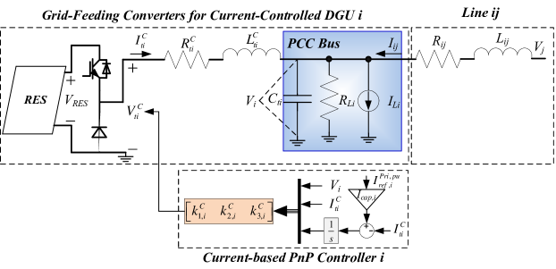
Figure 1: Electrical Scheme of CDGU $i$ and current-based PnP controller.

Remark 1.

In practical, the grid-feeding converters need the voltage support from the grid-forming converters at the PCC point. In this section, only the controller and stability for the interconnected CDGU is designed and analyzed. Thus, it is assumed that the voltage at the PCC point has already been supported by the grid-forming devices. In section 4 and 5, the PnP controllers to achieve both the voltage support and current feeding are proposed, designed and analyzed.

2.2 State-space model of multiple CDGUs

Dynamics (1) provides the state-space equations:

$$\text{ ${\Sigma}_{[i]}^{CDGU}:$}\left\{\begin{aligned} {\dot{x}}_{[i]}^{C}(t)&=A_{ii}^{C}{x}_{[i]}^{C}(t)+B_{i}^{C}{u}_{[i]}^{C}(t)+M_{i}^{C}{d}_{[i]}^{C}(t)+{\xi}_{[i]}^{C}(t)+A_{load,i}^{C}{x}_{[i]}^{C}(t)\\ {z}_{[i]}^{C}(t)&=H_{i}^{C}{x}_{[i]}^{C}(t)\\ \end{aligned}\right.$$

where ${x}_{[i]}^{C}=[V_{i},I_{ti}^{C}]^{T}$ is the state, ${u}_{[i]}^{C}=V_{ti}^{C}$ the control input, ${d}_{[i]}^{C}=I_{Li}^{C}$ the exogenous input including different current loads and ${z}_{[i]}^{C}=I_{ti}^{C}$ the controlled variable of the system. The term ${\xi}_{[i]}^{C}=\sum_{j\in{\mathcal{N}}_{i}}A_{ij}^{C}({x}_{[j]}^{C}-{x}_{[i]}^{C})$ accounts for the coupling with each CDGU $j\in{\mathcal{N}}_{i}^{C}$ and the term $A_{load,i}^{C}$ accounts for the resistive load for each CDGU. The matrices of ${\Sigma}_{[i]}^{CDGU}$ are obtained from (1) as:

$$A_{ii}^{C}=\begin{bmatrix}0&\frac{1}{C_{ti}}\\ -\frac{1}{L_{ti}^{C}}&-\frac{R_{ti}^{C}}{L_{ti}^{C}}\\ \end{bmatrix},\hskip 8.53581ptA_{load,i}^{C}=\begin{bmatrix}-\frac{1}{R_{Li}C_{ti}}&0\\ 0&0\end{bmatrix},\hskip 8.53581ptA_{ij}^{C}=\begin{bmatrix}\frac{1}{R_{ij}C_{ti}}&0\\ 0&0\end{bmatrix},$$

$$B_{i}^{C}=\begin{bmatrix}0\\ \frac{1}{L_{ti}^{C}}\end{bmatrix},\qquad M_{i}^{C}=\begin{bmatrix}-\frac{1}{C_{ti}}\\ 0\\ \end{bmatrix},\qquad H_{i}^{C}=\begin{bmatrix}0&1\end{bmatrix}.$$

Remark 2.

To be emphasized, there are two main differences between the proposed model for CDGU in (1) and the one proposed in [11]. The first one is that the resistive load is considered as part of the load. The second one is that the control variable is changed from voltage in [11] for grid-forming converters to current in (1) for grid-feeding converters.

The overall model with multiple CDGUs is given by

$$\mathbf{\dot{x}^{C}}(t) =\mathbf{A^{C}x^{C}}(t)+\mathbf{B^{C}u^{C}}(t)+\mathbf{M^{C}d^{C}}(t)$$ (2)

$$\mathbf{z}^{C}(t) =\mathbf{H^{C}x^{C}}(t)$$

where $\mathbf{x^{C}}=({x}_{[1]}^{C},\ldots,{x}_{[N]}^{C})\in\mathbb{R}^{2N}$, $\mathbf{u^{C}}=({u}_{[1]}^{C},\ldots,{u}_{[N]}^{C})\in\mathbb{R}^{N}$, $\mathbf{d^{C}}=({d}_{[1]}^{C},\ldots,{d}_{[N]}^{C})\in\mathbb{R}^{N}$, $\mathbf{z^{C}}=({z}_{[1]}^{C},\ldots,{z}_{[N]}^{C})\in\mathbb{R}^{N}$. Matrices $\mathbf{A^{C}}$, $\mathbf{B^{C}}$, $\mathbf{M^{C}}$ and $\mathbf{H^{C}}$ are reported in Appendix A.1.

3 Design of stabilizing current controllers

3.1 Structure of current-based PnP controllers

In order to track with references $\mathbf{z_{ref}^{C}}(t)$, when $\mathbf{d^{C}}(t)=\mathbf{\bar{d}^{C}}$ is constant, the CDGU model is augmented with integrators [19]. A necessary condition for making error $\mathbf{e^{C}}(t)=\mathbf{z_{ref}^{C}}(t)-\mathbf{z^{C}}(t)$ equal to zero as $t\rightarrow\infty$, is that, there are equilibrium states and inputs $\mathbf{\bar{x}^{C}}$ and $\mathbf{\bar{u}^{C}}$ verifying (2). The existence of these equilibrium points can be shown following the proof of Proposition 1 in [10].

One obtain the integrator dynamics is (as shown in Fig. 1, setting $z_{ref_{[i]}}^{C}=I_{ref,i}^{Pri,pu}*I_{cap,i}$, $I_{cap,i}$ is the maximum capability of CDGU $i$ and $I_{ref,i}^{Pri,pu}$ is the p.u. reference)

$${\dot{v}}_{[i]}^{C}(t)={e}_{[i]}^{C}(t) ={z_{ref}}_{[i]}^{C}(t)-{z}_{[i]}^{C}(t)$$ (3)

$$={z_{ref}}_{[i]}^{C}(t)-H_{i}^{C}{x}_{[i]}^{C}(t),$$

and hence, the augmented CDGU model is

$${\hat{\Sigma}}_{[i]}^{CDGU}:\left\{\begin{aligned} {\dot{\hat{x}}}_{[i]}^{C}(t)&=\hat{A}_{ii}^{C}{\hat{x}}_{[i]}^{C}(t)+\hat{B}_{i}^{C}{u}_{[i]}^{C}(t)+\hat{M}_{i}^{C}{\hat{d}}_{[i]}^{C}(t)+{\hat{\xi}}_{[i]}^{C}(t)+\hat{A}_{load,i}^{C}{\hat{x}}_{[i]}^{C}(t)\\ {z}_{[i]}^{C}(t)&=\hat{H}_{i}^{C}{\hat{x}}_{[i]}^{C}(t)\end{aligned}\right.$$ (4)

where ${\hat{x}}_{[i]}^{C}=[[{x}_{[i]}^{C}]^{T},{v}_{[i]}^{C}]^{T}\in\mathbb{R}^{3}$ is the state, ${\hat{d}}_{[i]}^{C}=[{d}_{[i]}^{C},{z_{ref}}_{[i]}^{C}]^{T}\in\mathbb{R}^{2}$ collects the exogenous signals and ${\hat{\xi}}_{[i]}^{C}=\sum_{j\in{\mathcal{N}}_{i}}\hat{A}_{ij}^{C}({\hat{x}}_{[j]}^{C}-{\hat{x}}_{[i]}^{C})$. By direct calculation, the matrices appeared in (4) are as follows

$$\hat{A}_{ii}^{C} =\begin{bmatrix}A_{ii}^{C}&0\\ -H_{i}^{C}&0\end{bmatrix},\hskip 5.69054pt\hat{A}_{ij}^{C}=\begin{bmatrix}A_{ij}^{C}&0\\ 0&0\end{bmatrix},\hskip 5.69054pt\hat{A}_{load,i}^{C}=\begin{bmatrix}A_{load,i}^{C}&0\\ 0&0\end{bmatrix},$$

$$\hat{B}_{i}^{C} =\begin{bmatrix}B_{i}^{C}\\ 0\end{bmatrix},\hskip 5.69054pt\hat{M}_{i}^{C}=\begin{bmatrix}M_{i}^{C}&0\\ 0&1\end{bmatrix},\hskip 5.69054pt\hat{H}_{i}^{C}=\begin{bmatrix}H_{i}^{C}&0\end{bmatrix}.$$

Based on Proposition 2 of [10], the pair $(\hat{A}_{ii}^{C},\hat{B}_{i}^{C})$ can be proven to be controllable. Hence, system (4) can be stabilized.

Given from (4), the overall augmented system is

$$\left\{\begin{aligned} \mathbf{\dot{\hat{x}}^{C}}(t)&=\mathbf{\hat{A}^{C}\hat{x}^{C}}(t)+\mathbf{\hat{B}^{C}u^{C}}(t)+\mathbf{\hat{M}^{C}\hat{d}^{C}}(t)\\ \mathbf{z}^{C}(t)&=\mathbf{\hat{H}^{C}\hat{x}^{C}}(t)\end{aligned}\right.$$ (5)

where $\mathbf{\hat{x}^{C}}$ and $\mathbf{\hat{d}^{C}}$ include all variables ${\hat{x}}_{[i]}^{C}$ and ${\hat{d}}_{[i]}^{C}$ respectively from all the CDGUs, and matrices $\mathbf{\hat{A}^{C}},\mathbf{\hat{B}^{C}},\mathbf{\hat{M}^{C}}$ and $\mathbf{\hat{H}^{C}}$ are derived from systems (4).

Now each CDGU ${\hat{\Sigma}}_{[i]}^{CDGU}$ is equip with the following state-feedback controller

$${{\mathcal{C}}}_{[i]}^{C}:\qquad{u}_{[i]}^{C}(t)=K_{i}^{C}{\hat{x}}_{[i]}^{C}(t)$$ (6)

where $K_{i}^{C}=\left[k_{1,i}^{C}\text{ }k_{2,i}^{C}\text{ }k_{3,i}^{C}\right]\in\mathbb{R}^{1\times 3}$.

It turns out that, together with the integral action (3), controllers ${{\mathcal{C}}}_{[i]}^{C}$, define a multivariable PI regulator, see lower part of Fig. 1. In particular, the overall control architecture is decentralized since the computation of ${u}_{[i]}^{C}$ requires the state of ${\hat{\Sigma}}_{[i]}^{CDGU}$ only. In the following, it is shown that structured Lyapunov functions can be used to ensure asymptotic stability of the system with multiple CDGUs with controllers (6).

3.2 Conditions for stability of the closed-loop multiple CDGUs

As in [11], the design of gain $K_{i}^{C}$ hinges on the use of separable local Lyapunov function for certifying the closed-loop stability. Indeed, the structure will also allow us to show that local stability implies stability of the whole system. Here after, the candidate Lyapunov function are considered as

$$V_{i}^{C}({\hat{x}}_{[i]}^{C})=[{\hat{x}}_{[i]}^{C}]^{T}P_{i}^{C}{\hat{x}}_{[i]}^{C}$$ (7)

where positive definite matrices $P_{i}^{C}\in\mathbb{R}^{3\times 3}$ has the structure

$$P_{i}^{C}=\left[\begin{array}[]{c|c}\eta_{i}&\mathbf{0}_{1\times 2}\\ \hline\cr\mathbf{0}_{2\times 1}&{\mathcal{P}}_{22,i}^{C}\\ \end{array}\right],$$ (8)

where $\eta_{i}>0$ is a parameter and the entries of ${\mathcal{P}}_{22,i}^{C}$ are arbitrary and denoted as

$${\mathcal{P}}_{22,i}^{C}=\left[\begin{array}[]{cc}p_{22,i}^{C}&p_{23,i}^{C}\\ p_{23,i}^{C}&p_{33,i}^{C}\end{array}\right].$$ (9)

We also assume that given a constant parameter common to all CDGUs $\bar{\sigma}>0$ just for proof process, the parameters $\eta_{i}$ in (8) are set as

$$\eta_{i}=\bar{\sigma}C_{ti}\hskip 19.91692pti\in{\mathcal{D}}^{C}.$$ (10)

In absence of coupling terms ${\hat{\xi}}_{[i]}^{C}(t)$, and load terms $\hat{A}_{load,i}^{C}{\hat{x}}_{[i]}^{C}(t)$, one would like to stabilize the closed-loop CDGU

$${\dot{\hat{x}}}_{[i]}^{C}(t)=\underbrace{(\hat{A}_{ii}^{C}+\hat{B}_{i}^{C}K_{i}^{C})}_{F_{i}^{C}}{\hat{x}}_{[i]}^{C}(t)+\hat{M}_{i}^{C}{{\hat{d}}}_{[i]}^{C}(t).\\$$ (11)

By direct calculation, one has

$$F_{i}^{C}=\left[\begin{array}[]{c|cc}0&\frac{1}{C_{t}}&0\\ \hline\cr\frac{(k_{1,i}^{C}-1)}{L_{ti}^{C}}&\frac{(k_{2,i}^{C}-R_{ti}^{C})}{L_{ti}^{C}}&\frac{k_{3,i}^{C}}{L_{ti}^{C}}\\ 0&-1&0\end{array}\right]=\left[\begin{array}[]{c|cc}0&{\mathcal{F}}_{12,i}^{C}\\ \hline\cr{\mathcal{F}}_{21,i}^{C}&{\mathcal{F}}_{22,i}^{C}\end{array}\right].$$ (12)

From Lyapunov theory, asymptotic stability of (11) can be certified by the existence of a Lyapunov function as shown in (7) and

$$Q_{i}^{C}=[F_{i}^{C}]^{T}P_{i}^{C}+P_{i}^{C}F_{i}^{C}$$ (13)

is negative definite.

Based on (8) and (12), eq. (13) can be rewritten as

$$Q_{i}^{C}=\left[\begin{array}[]{c|cc}0&[{\mathcal{F}}_{21,i}^{C}]^{T}{\mathcal{P}}_{22,i}^{C}+\eta_{i}{\mathcal{F}}_{12,i}^{C}\\ \hline\cr[{\mathcal{F}}_{12,i}^{C}]^{T}\eta_{i}+{\mathcal{P}}_{22,i}^{C}{\mathcal{F}}_{21,i}^{C}&[{\mathcal{F}}_{22,i}^{C}]^{T}{\mathcal{P}}_{22,i}^{C}+{\mathcal{P}}_{22,i}^{C}{\mathcal{F}}_{22,i}^{C}\end{array}\right]$$ (14)

The next result shows that, Lyapunov theory certifies, at most, marginal stability of (11).

Firstly, we recall the following elementary properties of the positive definite matrix $P_{i}^{C}$ and the negative semi-definite matrix $Q_{i}^{C}$.

Proposition 1.

[11] If $Q=Q^{T}\leq 0$ and an element $q_{ii}$ on the diagonal verified $q_{ii}=0$, then

1. The matrix $Q$ cannot be negative definite.

2. The $i$-th row and column have zero entries.

Proposition 2.

Matrices $P_{i}^{C}>0$ and $Q_{i}^{C}\leq 0$ verifying (8) and (14) have the following structure:

$$P_{i}^{C}=\left[\begin{array}[]{c|cc}\eta_{i}&0&0\\ \hline\cr 0&p_{22,i}^{C}&0\\ 0&0&\frac{k_{3,i}^{C}}{L_{ti}^{C}}p_{22,i}^{C}\\ \end{array}\right],\hskip 14.22636ptQ_{i}^{C}=\left[\begin{array}[]{c|c|c}0&0&0\\ \hline\cr 0&2\frac{(k_{2,i}^{C}-R_{ti}^{C})}{L_{ti}^{C}}p_{22,i}^{C}&0\\ \hline\cr\ 0&0&0\\ \end{array}\right],$$ (15)

Moreover, for having $P_{i}^{C}>0$, $Q_{i}^{C}\leq 0$ and $Q_{i}^{C}\neq 0$, the control coefficients must verify

$$\left\{\begin{aligned} k_{1,i}^{C}&<1\\ k_{2,i}^{C}&<R_{ti}^{C}\\ k_{3,i}^{C}&>0\end{aligned}\right.$$ (16)

Proof.

Based on (9) and (12), the upper right block of (14) can be written as

$$[{\mathcal{F}}_{21,i}^{C}]^{T}{\mathcal{P}}_{22,i}^{C}+\eta_{i}{\mathcal{F}}_{12,i}^{C}=\left[\begin{array}[]{c|cc}\frac{(k_{1,i}^{C}-1)}{L_{ti}^{C}}p_{22,i}^{C}+\frac{1}{C_{ti}}\eta_{i}&\frac{(k_{1,i}^{C}-1)}{L_{ti}^{C}}p_{23,i}^{C}\end{array}\right],$$ (17)

Based on Proposition 1, (17) should be equal to zero vector which means

$$\frac{(k_{1,i}^{C}-1)}{L_{ti}^{C}}p_{22,i}^{C} =-\frac{1}{C_{ti}}\eta_{i}$$ (18a)

$$\frac{(k_{1,i}^{C}-1)}{L_{ti}^{C}}p_{23,i}^{C} =0$$ (18b)

Because $\eta_{i}$ is positive, one has

$$k_{1,i}^{C} <1$$ (19a)

$$p_{23,i}^{C} =0$$ (19b)

From (19), the lower right block of (14) can be rewritten as

$$[{\mathcal{F}}_{22,i}^{C}]^{T}{\mathcal{P}}_{22,i}^{C}+{\mathcal{P}}_{22,i}^{C}{\mathcal{F}}_{22,i}^{C}=\left[\begin{array}[]{c|cc}2\frac{(k_{2,i}^{C}-R_{ti}^{C})}{L_{ti}^{C}}p_{22,i}^{C}&-p_{33,i}^{C}+\frac{k_{3,i}^{C}}{L_{ti}^{C}}p_{22,i}^{C}\\ \hline\cr-p_{33,i}^{C}+\frac{k_{3,i}^{C}}{L_{ti}^{C}}p_{22,i}^{C}&0\\ \end{array}\right],$$ (20)

Again from Proposition 1, the off diagonal entities of (20) must be equal to zero which means

$$\frac{k_{3,i}^{C}}{L_{ti}^{C}}p_{22,i}^{C}=p_{33,i}^{C}\\$$ (21)

Furthermore, based on (19b), (21) and $P_{i}^{C}>0$

$$k_{3,i}^{C}>0\\$$ (22)

Finally, for verifying $Q_{i}^{C}\neq 0$, one has

$$k_{2,i}^{C}<R_{ti}^{C}\\$$ (23)

Thus, the $P_{i}^{C}$ in (15) can be derived by substituting (19b) and (21) into (8) and then $Q_{i}^{C}$ in (15) can be derived from (20) and (21), finally (19a), (23) and (22) consist of the set (16) for control coefficients. ∎

An immediate consequence of Proposition 2 is the following results which will be exploited for proving the stability of the whole system through the LaSalle theorem.

Lemma 1.

Let $g_{i}(w_{i})=w_{i}^{T}Q_{i}^{C}w_{i}$. Under the Proposition 2, $\forall i\in{\mathcal{D}}^{C}$, only vectors $\bar{w}_{i}$ in the form

$$\bar{w}_{i}=\left[\begin{array}[]{ccc}\alpha_{i}&0&\beta_{i}\end{array}\right]^{T}$$

with $\alpha_{i}$, $\beta_{i}\in\mathbb{R}$, fulfill

$$g_{i}(\bar{w}_{i})=\bar{w}_{i}^{T}Q_{i}^{C}\bar{w}_{i}=0.$$ (24)

Now the overall closed-loop model with multiple CDGUs is considered as

$$\left\{\begin{aligned} \mathbf{\dot{\hat{x}}}^{C}(t)&=(\mathbf{\hat{A}^{C}+\hat{B}^{C}K^{C}})\mathbf{\hat{x}}^{C}(t)+\mathbf{\hat{M}^{C}{\hat{d}}^{C}}(t)\\ \mathbf{z}^{C}(t)&=\mathbf{\hat{H}^{C}\hat{x}^{C}}(t)\end{aligned}\right.$$ (25)

obtained by combining (5) and (6), with $\mathbf{K}^{C}={\mbox{diag}}(K_{1}^{C},\dots,K_{N}^{C})$. Also the collective Lyapunov function

$${\mathcal{V}}^{C}(\mathbf{{\hat{x}}^{C}})=\sum_{i=1}^{N}{\mathcal{V}}_{i}^{C}(\hat{x}_{[i]}^{C})=\mathbf{[{\hat{x}}^{C}]}^{T}\mathbf{P^{C}}\mathbf{{\hat{x}}^{C}}$$ (26)

is considered, where $\mathbf{P^{C}}={\mbox{diag}}(P_{1}^{C},\dots,P_{N}^{C})$.

One has $\dot{\mathcal{V}}^{C}(\mathbf{{\hat{x}}^{C}})=\mathbf{[{\hat{x}}^{C}]}^{T}\mathbf{Q^{C}}\mathbf{{\hat{x}}^{C}}$ where

$$\mathbf{Q}^{C}=(\mathbf{\hat{A}^{C}}+\mathbf{\hat{B}^{C}K^{C}})^{T}\mathbf{P^{C}}+\mathbf{P^{C}}(\mathbf{\hat{A}^{C}}+\mathbf{\hat{B}^{C}K^{C}}).$$

A consequence of Proposition 2 is that, the matrix $\mathbf{Q^{C}}$ cannot be negative definite. At most, one has

$$\mathbf{Q^{C}}\leq 0.$$ (27)

Moreover, even if $Q_{i}^{C}\leq 0$ holds for all $i\in{\mathcal{D}}^{C}$, the inequality (27) might be violated because of the nonzero coupling terms $\hat{A}_{ij}^{C}$ and load terms $\hat{A}_{load,i}^{C}$ in matrix $\mathbf{\hat{A}}$. The next result shows that this cannot happen if (10) holds.

Proposition 3.

If gains $K_{i}^{C}$ are chosen according to the (16) in Proposition 2 and (10) holds, then (27) holds.

Proof.

Consider the following decomposition of matrix $\mathbf{\hat{A}^{C}}$

$$\mathbf{\hat{A}^{C}}=\mathbf{\hat{A}_{D}^{C}}+\mathbf{\hat{A}_{\Xi}^{C}}+\mathbf{\hat{A}_{L}^{C}}+\mathbf{\hat{A}_{C}^{C}},$$ (28)

where $\mathbf{\hat{A}_{D}^{C}}={\mbox{diag}}(\hat{A}_{ii}^{C},\dots,\hat{A}_{NN}^{C})$ collects the local dynamics only, $\mathbf{\hat{A}_{C}^{C}}$ collects the coupling dynamic representing the off-diagonal items of matrix $\mathbf{\hat{A}^{C}}$, while $\mathbf{\hat{A}_{\Xi}^{C}}={\mbox{diag}}(\hat{A}_{\xi 1}^{C},\dots,\hat{A}_{\xi N}^{C})$ and $\mathbf{\hat{A}_{L}^{C}}={\mbox{diag}}(\hat{A}_{load,1}^{C},\dots,\hat{A}_{load,N}^{C})$ with

$$\hat{A}_{\xi i}^{C}=\begin{bmatrix}-\sum\limits_{j\in{\mathcal{N}}_{i}}\frac{1}{R_{ij}C_{ti}}&0&0\\ 0&0&0\\ 0&0&0\end{bmatrix},\hat{A}_{load,i}^{C}=\begin{bmatrix}-\frac{1}{R_{Li}C_{ti}}&0&0\\ 0&0&0\\ 0&0&0\end{bmatrix},$$

takes into account the dependence of each local state on the neighboring CDGUs and the local resistive load. According to the decomposition (28), the inequality (27) is equivalent to

$$\underbrace{\mathbf{(\hat{A}_{D}^{C}+\hat{B}^{C}K^{C})^{T}P^{C}+P^{C}(\hat{A}_{D}^{C}+\hat{B}^{C}K^{C})}}_{({a})}+\underbrace{\mathbf{2({\hat{A}_{\Xi}^{C}}+\mathbf{\hat{A}_{L}^{C}})P^{C}}}_{(b)}+\underbrace{\mathbf{(\hat{A}_{C}^{C})^{T}P^{C}+P^{C}\hat{A}_{C}}}_{(c)}\leq 0.$$ (29)

By means of $Q_{i}^{C}\leq 0$, matrix $(a)=\mathrm{diag}(Q_{1}^{C},\dots,Q_{N}^{C})$ is negative semidefinite. Then the contribution of $(b)+(c)$ in (29) is studied. Matrix $(b)$, by construction, is block diagonal and collects on its diagonal blocks in the form

$$2({\hat{A}_{\xi i}^{C}}+\hat{A}_{load,i}^{C})P_{i}^{C} =\begin{bmatrix}-2\frac{1}{R_{Li}C_{ti}}-2\sum\limits_{j\in{\mathcal{N}}_{i}}\frac{1}{R_{ij}C_{ti}}&0&0&\\ 0&0&0\\ 0&0&0\\ \end{bmatrix}\left[\begin{array}[]{c|c}\eta_{i}&\mathbf{0}_{1\times 2}\\ \hline\cr\mathbf{0}_{2\times 1}&{\mathcal{P}}_{22,i}^{C}\end{array}\right]=$$ (30)

$$=\begin{bmatrix}-2\tilde{\eta}_{i}-2\sum\limits_{j\in{\mathcal{N}}_{i}}\tilde{\eta}_{ij}&0&0\\ 0&0&0\\ 0&0&0\\ \end{bmatrix},$$

where

$$\tilde{\eta}_{ij}=\frac{\eta_{i}}{R_{ij}C_{ti}},\text{ }\tilde{\eta}_{Li}=\frac{\eta_{i}}{R_{Li}C_{ti}}$$ (31)

Considering matrix $(c)$, each the block in position $(i,j)$ is equal to

$$\left\{\begin{array}[]{ll}P_{i}^{C}\hat{A}_{ij}^{C}+(\hat{A}_{ji}^{C})^{T}P_{j}^{C}&\hskip 19.91692pt\mbox{if }j\in\mathcal{N}_{i}\\ 0&\hskip 19.91692pt\mbox{otherwise}\end{array}\right.$$

where

$$P_{i}^{C}\hat{A}_{ij}^{C}+(\hat{A}_{ji}^{C})^{T}P_{j}^{C} =\begin{bmatrix}\tilde{\eta}_{ij}+\tilde{\eta}_{ji}&0&0\\ 0&0&0\\ 0&0&0\\ \end{bmatrix}.$$ (32)

From (30) and (32), except for the elements in position $(1,1)$ of each $3\times 3$ block of $(b)+(c)$, others are equals to zero. Thus, to evaluate the positive/negative definiteness of the matrix $(b)+(c)$, the $N\times N$ matrix can be equivalently considered by deleting the second and third rows and columns as

$${\mathcal{L}}^{C}=\left[\begin{array}[]{cccc}(-2\tilde{\eta}_{1}-2\sum\limits_{j\in{\mathcal{N}}_{1}}\tilde{\eta}_{1j})&\bar{\eta}_{12}&\dots&\bar{\eta}_{1N}\\ \bar{\eta}_{21}&\ddots&\ddots&\vdots\\ \vdots&\ddots&(-2\tilde{\eta}_{N-1}-2\sum\limits_{j\in{\mathcal{N}}_{N-1}}\tilde{\eta}_{N-1j})&\bar{\eta}_{N-1N}\\ \bar{\eta}_{N1}&\dots&\bar{\eta}_{NN-1}&(-2\tilde{\eta}_{N}-2\sum\limits_{j\in{\mathcal{N}}_{N}}\tilde{\eta}_{Nj})\end{array}\right]$$ (33)

One has ${\mathcal{L}}^{C}={\mathcal{M}}^{C}+{\mathcal{U}}^{C}+{\mathcal{G}}^{C}$, where

$$\mathcal{M^{C}}=\begin{bmatrix}-2\sum\limits_{j\in{\mathcal{N}}_{1}}\tilde{\eta}_{1j}&0&\dots&0\\ 0&-2\sum\limits_{j\in{\mathcal{N}}_{2}}\tilde{\eta}_{2j}&\ddots&\vdots\\ \vdots&\ddots&\ddots&0\\ 0&\dots&0&-2\sum\limits_{j\in{\mathcal{N}}_{N}}\tilde{\eta}_{Nj}\end{bmatrix},\mathcal{U^{C}}=\begin{bmatrix}-2\tilde{\eta}_{L1}&0&\dots&0\\ 0&-2\tilde{\eta}_{L2}&\ddots&\vdots\\ \vdots&\ddots&\ddots&0\\ 0&\dots&0&-2\tilde{\eta}_{LN}\end{bmatrix},$$

and

$$\mathcal{G^{C}}=\left[\begin{array}[]{cccc}0&\bar{\eta}_{12}&\dots&\bar{\eta}_{1N}\\ \bar{\eta}_{21}&0&\ddots&\vdots\\ \vdots&\ddots&\ddots&\bar{\eta}_{N-1N}\\ \bar{\eta}_{N1}&\dots&\bar{\eta}_{NN-1}&0\end{array}\right].$$ (34)

Notice that each off-diagonal element $\bar{\eta}_{ij}$ in (34) is equal to

$$\bar{\eta}_{ij}=\left\{\begin{array}[]{ll}(\tilde{\eta}_{ij}+\tilde{\eta}_{ji})&\hskip 19.91692pt\mbox{if }j\in\mathcal{N}_{i}\\ 0&\hskip 19.91692pt\mbox{otherwise}\end{array}\right.$$ (35)

At this point, from (10), one obtains that $\tilde{\eta}_{ij}=\tilde{\eta}_{ji}$ (see (31)) and, consequently, $\bar{\eta}_{ij}=\bar{\eta}_{ji}=2\tilde{\eta}_{ij}$ (see (35)). Hence, ${\mathcal{L}}^{C}$ is symmetric and has non negative off-diagonal elements. It follows that $-{\mathcal{L}}^{C}$ is equal to a Laplacian matrix [20, 21] plus an positive definite diagonal matrix. Thus, it verifies ${\mathcal{L}}^{C}<0$ by construction. By adding the deleted second and third rows and columns in each block of $(b)+(c)$, then (29) holds. ∎

Our next goal is to show asymptotic stability of the system with multiple CDGUs using the marginal stability result in Proposition 3 together with LaSalle invariance theorem. To this purpose, the main result is then given in Theorem 1 which relies on characterizing states $\mathbf{\hat{x}^{C}}$ deriving $\dot{\mathcal{V}}^{C}(\mathbf{\hat{x}}^{C})=0$.

Theorem 1.

If (10) holds and $Q_{i}^{C}\neq 0$ and the connectivity of the graph ${\mathcal{G}}_{el}$ is guaranteed, control coefficients are chosen according to (16), the origin of (25) is asymptotically stable.

Proof.

From Proposition 3, $\dot{\mathcal{V}}^{C}(\mathbf{\hat{x}}^{C})$ is negative semidefinite meaning that (27) holds. We aim at showing that the origin of the system with multiple CDGUs is also attractive using the LaSalle invariance Theorem [22]. For this purpose, the set is computed $R^{C}=\{\mathbf{x}^{C}\in\mathbb{R}^{3N}:(\mathbf{x^{C}})^{T}\mathbf{Q^{C}}\mathbf{x^{C}}=0\}$ by means of the decomposition in (29), which coincides with

$$R^{C} =\{\mathbf{x^{C}}:\mathbf{(x^{C})}^{T}\left((a)+(b)+(c)\right)\mathbf{x^{C}}=0\}$$ (36)

$$=\{\mathbf{x^{C}}:\mathbf{(x^{C})}^{T}(a)\mathbf{x^{C}}+\mathbf{(x^{C})}^{T}(b)\mathbf{x^{C}}+\mathbf{(x^{C})}^{T}(c)\mathbf{x^{C}}=0\}$$

$$=\underbrace{\{\mathbf{x^{C}}:\mathbf{(x^{C})}^{T}(a)\mathbf{x^{C}}=0\}}_{X_{1}^{C}}\cap\underbrace{\{\mathbf{x^{C}}:\mathbf{(x^{C})}^{T}\left[(b)+(c)\right]\mathbf{x^{C}}=0\}}_{X_{2}^{C}}.$$

In particular, the last equality follows from the fact that $(a)$ and $(b)+(c)$ are negative semidefinite matrices (see the proof of Proposition 3).

First, based on Lemma 1, the set $X_{1}^{C}$ is characterized as

$$X_{1}^{C}=\{\mathbf{x^{C}}:\mathbf{x^{C}}=\left[\text{ }\alpha_{1}\text{ }0\text{ }\beta_{1}\text{ }|\text{ }\cdots\text{ }|\text{ }\alpha_{N}\text{ }0\text{ }\beta_{N}\text{ }\right]^{T},\alpha_{i},\beta_{i}\in\mathbb{R}\},$$ (37)

Then, we focus on the elements of set $X_{2}^{C}$ based on Proposition 3. Since matrix $(b)+(c)$ can be seen as an ”expansion” of a matrix which is negative definite matrix with zero entries on the second and third rows and columns of $3\times 3$ block, by construction, vectors in the form

$$X_{2}^{C}=\{\mathbf{x^{C}}:\mathbf{x^{C}}=\left[\text{ }0\text{ }\tilde{x}_{12}\text{ }\tilde{x}_{13}\text{ }|\text{ }\cdots\text{ }|\text{ }0\text{ }\tilde{x}_{N2}\text{ }\tilde{x}_{N3}\text{ }\right]^{T},\tilde{x}_{i2},\tilde{x}_{i3}\in\mathbb{R}\},$$ (38)

Hence, by merging (37) and (38), and from (36), it derives that

$$R^{C}=\{\mathbf{x}:\mathbf{x}=\left[\text{ }0\text{ }0\text{ }\beta_{1}\text{ }|\text{ }\cdots\text{ }|\text{ }0\text{ }0\text{ }\beta_{N}\text{ }\right]^{T},\beta_{i}\in\mathbb{R}\}.$$ (39)

Finally, in order to conclude the proof, it should be shown that the largest invariant set $M^{C}\subseteq R$ is the origin. To this purpose, (11) is considered, by adding the coupling terms ${\hat{\xi}}_{[i]}$ and the resistance load term $\hat{A}_{load,i}^{C}\hat{x}_{i}^{C}(0)$, setting load disturbance $\hat{d}_{[i]}^{C}=0$, choosing the initial state $\mathbf{\hat{x}}^{C}(0)=\left[\hat{x}_{1}^{C}(0)|\dots|\hat{x}_{N}^{C}(0)\right]^{T}\in R^{C}$. In order to find conditions on the elements of $\mathbf{\hat{x}}^{C}(0)$ that must hold for having $\mathbf{\dot{\hat{x}}^{C}}\in R^{C}$, one has

$$\dot{\hat{x}}_{i}^{C}(0) ={F_{i}^{C}}\hat{x}_{i}^{C}(0)+\hat{A}_{load,i}^{C}\hat{x}_{i}^{C}(0)+\sum\limits_{j\in{\mathcal{N}}_{i}}\underbrace{\hat{A}_{ij}^{C}\left(\hat{x}_{j}^{C}(0)-\hat{x}_{i}^{C}(0)\right)}_{=0}$$

$$=\left[\begin{array}[]{ccc}-\frac{1}{R_{Li}C_{ti}}&\frac{1}{C_{ti}}&0\vspace{2mm}\\ \frac{k_{1,i}^{C}-1}{L_{ti}^{C}}&\frac{k_{2,i}^{C}-R_{ti}^{C}}{L_{ti}^{C}}&\frac{k_{3,i}^{C}}{L_{ti}^{C}}\vspace{2mm}\\ 0&-1&0\\ \end{array}\right]\left[\begin{array}[]{c}0\vspace{2mm}\\ 0\vspace{2mm}\\ \beta_{i}\end{array}\right]$$

$$=\left[\begin{array}[]{c}0\vspace{2mm}\\ \frac{k_{3,i}^{C}}{L_{ti}^{C}}\beta_{i}\vspace{2mm}\\ 0\end{array}\right]\normalsize$$

for all $i\in{\mathcal{D}}^{C}$. It follows that $\mathbf{\dot{\hat{x}}^{C}}(0)\in R$ only if $\beta_{i}=0$. Since $M^{C}\subseteq R$, from (39) one has $M^{C}=\{0\}$. ∎

Remark 3.

The design of stabilizing controller for each CDGU can be conducted according to Proposition 2. In particular, differently from the approach in [11], no optimization problem has to be solved for computing a local controller. Indeed, it is enough to choose control coefficient $k_{1,i}^{C}$, $k_{2,i}^{C}$ and $k_{3,i}^{C}$ from inequality set (16). Note that these inequalities are always feasible, implying that a stabilizing controller always exists. Moreover, the inequalities depend only on the parameter $R_{ti}^{C}$ of the CDGU $i$. Therefore, the control synthesis is independent of parameters of CDGUs and power lines which means that controller design can be executed only once for each CDGU in a plug-and play fashion. From Theorem 1, local controllers also guarantee stability of the whole MG. When new CDGUs are plugged in the MG, their controller are designed as described above, the connectivity of the electrical graph ${\mathcal{G}}_{el}$ is preserved and have Theorem 1 applied to the whole MG. Instead, when a CDGU is plugged out, the electrical graph ${\mathcal{G}}_{el}$ might be disconnected and split into two connected graphs. Theorem 1 can still be applied to show the stability of each sub-MG.

4 DC MG with Grid-Forming/Feeding Converters and Its Clusters

4.1 Electrical model of one MG

As mentioned before, the CDGU should be cooperative operated with voltage support in the MGs. The ESS is interfaced with the MG by means of the grid-forming converter of VDGU to provide necessary voltage support for the PCC bus based on which, the RES is interfaced with the MG through the grid-feeding converters of CDGU to provide current for the loads. Thus, in this section, the combination of oen VDGU and one CDGU is considered as one MG through connecting to the same common bus achieving both voltage support and current feeding simultaneously. And the MG clusters are formed by interconnecting several MGs through line impedances.

Here, a MG cluster system composed of $N$ MGs is considered belonging to set ${\mathcal{D}}=\{1,\dots,N\}$. Two MGs are neighbors if there is a power line connecting them. ${\mathcal{N}}_{i}\subset{\mathcal{D}}$ denotes the subset of neighbors of MG $i$. The neighboring relation is symmetric which means $j\in{\mathcal{N}}_{i}$ implies $i\in{\mathcal{N}}_{j}$.

The electrical scheme of the $i$-th MG is represented with Fig. 2

$$\text{Module}~{}i:\quad\left\{\begin{aligned} \frac{dV_{i}}{dt}&=\frac{1}{C_{ti}}I_{ti}^{C}+\frac{1}{C_{ti}}I_{ti}^{V}+\sum\limits_{j\in{\mathcal{N}}_{i}}\left(\frac{V_{j}}{C_{ti}R_{ij}}-\frac{V_{i}}{C_{ti}R_{ij}}\right)-\frac{1}{C_{ti}}(I_{Li}+\frac{V_{i}}{R_{Li}})\\ \frac{dI_{ti}^{C}}{dt}&=-\frac{1}{L_{ti}^{C}}V_{i}-\frac{R_{ti}^{C}}{L_{ti}^{C}}I_{ti}^{C}+\frac{1}{L_{ti}^{C}}V_{ti}^{C}\\ \frac{dI_{ti}^{V}}{dt}&=-\frac{1}{L_{ti}^{V}}V_{i}-\frac{R_{ti}^{V}}{L_{ti}^{V}}I_{ti}^{V}+\frac{1}{L_{ti}^{V}}V_{ti}^{V}\\ \end{aligned}\right.$$ (40)

where variables $V_{i}$, $I_{ti}^{C}$, $I_{ti}^{V}$ are the $i$-th PCC voltage and filter current from RES and filter current from ESS, respectively, $V_{ti}^{C}$ represents the command to the grid-feeding converter, $V_{ti}^{V}$ represents the command to the grid-forming converter, and $R_{ti}^{C}$, $L_{ti}^{C}$ the electrical parameters for grid-feeding converter, $R_{ti}^{V}$, $L_{ti}^{V}$ the electrical parameters for grid-forming converter, $C_{ti}$ is the capacitor at the common PCC bus. Moreover, $V_{j}$ is the voltage at the PCC of each neighboring MG $j\in{\mathcal{N}}_{i}$ and $R_{ij}$ and $L_{ij}$ is the resistance and inductance of the power DC line connecting MGs $i$ and $j$.

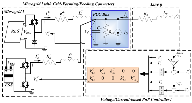
Figure 2: Electrical Scheme of MG $i$ and voltage/current-based PnP controller.

4.2 State-space model of MG clusters

Dynamics (40) provides the state-space variables equations:

$$\text{ ${\Sigma}_{[i]}^{MG}:$}\left\{\begin{aligned} {\dot{x}}_{[i]}(t)&=A_{ii}{x}_{[i]}(t)+B_{i}{u}_{[i]}(t)+M_{i}{d}_{[i]}(t)+{\xi}_{[i]}(t)+A_{load,i}{x}_{[i]}(t)\\ {z}_{[i]}(t)&=H_{i}{x}_{[i]}(t)\\ \end{aligned}\right.$$

where ${x}_{[i]}=[V_{i},I_{ti}^{C},I_{ti}^{V}]^{T}$ is the state of the system, ${u}_{[i]}=[V_{ti}^{C},V_{ti}^{V}]$ is the control input, ${d}_{[i]}=I_{Li}$ is the exogenous input and ${z}_{[i]}=[I_{i}^{C},V_{i}]$ is the controlled variable of the system. The term ${\xi}_{[i]}=\sum_{j\in{\mathcal{N}}_{i}}A_{ij}({x}_{[j]}-{x}_{[i]})$ accounts for the coupling with each MG $j\in{\mathcal{N}}_{i}$. The matrices of ${\Sigma}_{[i]}^{MG}$ are obtained from (40) as:

$$A_{ii}=\begin{bmatrix}0&\frac{1}{C_{ti}}&\frac{1}{C_{ti}}\\ -\frac{1}{L_{ti}^{C}}&-\frac{R_{ti}^{C}}{L_{ti}^{C}}&0\\ -\frac{1}{L_{ti}^{V}}&0&-\frac{R_{ti}^{V}}{L_{ti}^{V}}\\ \end{bmatrix},\hskip 8.53581ptA_{load,i}=\begin{bmatrix}-\frac{1}{R_{Li}C_{ti}}&0&0\\ 0&0&0\\ 0&0&0\\ \end{bmatrix},\hskip 8.53581ptA_{ij}=\begin{bmatrix}\frac{1}{R_{ij}C_{ti}}&0&0\\ 0&0&0\\ 0&0&0\\ \end{bmatrix},$$

$$B_{i}=\begin{bmatrix}0&0\\ \frac{1}{L_{ti}^{C}}&0\\ 0&\frac{1}{L_{ti}^{V}}\end{bmatrix},\qquad M_{i}=\begin{bmatrix}-\frac{1}{C_{ti}}\\ 0\\ 0\\ \end{bmatrix},\qquad H_{i}=\begin{bmatrix}0&1&0\\ 1&0&0\\ \end{bmatrix}.$$

The overall model of MG clusters is given by

$$\mathbf{\dot{x}}(t) =\mathbf{Ax}(t)+\mathbf{Bu}(t)+\mathbf{Md}(t)$$ (41)

$$\mathbf{z}(t) =\mathbf{Hx}(t)$$

where $\mathbf{x}=({x}_{[1]},\ldots,{x}_{[N]})\in\mathbb{R}^{3N}$, $\mathbf{u}=({u}_{[1]},\ldots,{u}_{[N]})\in\mathbb{R}^{2N}$, $\mathbf{d^{C}}=({d}_{[1]},\ldots,{d}_{[N]})\in\mathbb{R}^{N}$, $\mathbf{z}=({z}_{[1]},\ldots,{z}_{[N]})\in\mathbb{R}^{2N}$. Matrices $\mathbf{A}$, $\mathbf{B}$, $\mathbf{M}$ and $\mathbf{H}$ are reported in Appendix A.2.

5 Design of stabilizing voltage/current controllers

5.1 Structure of PnP Voltage/Current controllers

In order to track constant references $\mathbf{z_{ref}}(t)$, when $\mathbf{d}(t)$ is constant as well, the MG model is augmented with integrators [19]. A necessary condition for making error $\mathbf{e}(t)=\mathbf{z_{ref}}(t)-\mathbf{z}(t)$ equal to zero as $t\rightarrow\infty$, is that, for arbitrary $\mathbf{\bar{d}}$ and $\mathbf{\bar{z}_{ref}}$, there are equilibrium states and inputs $\mathbf{\bar{x}}$ and $\mathbf{\bar{u}}$ verifying (41). The existence of these equilibrium points can be proven by following the proof of Proposition 1 in [10].

The dynamics of integrators are (as shown in Fig. 2, where $z_{ref_{[i]}}^{Pri,C}=I_{ref,i}^{Pri,pu}*I_{cap,i}$ , $z_{ref_{[i]}}^{Pri,V}={V_{ref,i}^{Pri}}$)

$${\dot{v}}_{[i]}^{C}(t) ={e}_{[i]}^{C}(t)=z_{ref_{[i]}}^{Pri,C}(t)-I_{ti}^{C}(t)$$ (42a)

$${\dot{v}}_{[i]}^{V}(t) ={e}_{[i]}^{V}(t)=z_{ref_{[i]}}^{Pri,V}(t)-V_{i}(t)$$ (42b)

and hence, the augmented model is

$${\hat{\Sigma}}_{[i]}^{MG}:\left\{\begin{aligned} {\dot{\hat{x}}}_{[i]}(t)&=\hat{A}_{ii}{\hat{x}}_{[i]}(t)+\hat{B}_{i}{u}_{[i]}(t)+\hat{M}_{i}{\hat{d}}_{[i]}(t)+{\hat{\xi}}_{[i]}(t)+\hat{A}_{load,i}{\hat{x}}_{[i]}(t)\\ {z}_{[i]}(t)&=\hat{H}_{i}{\hat{x}}_{[i]}(t)\end{aligned}\right.$$ (43)

where ${\hat{x}}_{[i]}=[V_{i},I_{ti}^{C},v_{i}^{C},I_{ti}^{V},v_{i}^{V}]^{T}\in\mathbb{R}^{5}$ is the state, ${\hat{d}}_{[i]}=[{d}_{[i]},{z_{ref}}_{[i]}^{Pri,C},{z_{ref}}_{[i]}^{Pri,V}]^{T}\in\mathbb{R}^{3}$ collects the exogenous signals and ${\hat{\xi}}_{[i]}=\sum_{j\in{\mathcal{N}}_{i}}\hat{A}_{ij}({\hat{x}}_{[j]}-{\hat{x}}_{[i]})$. Matrices in (43) are defined as follows

$$\hat{A}_{ii} =\begin{bmatrix}0&\frac{1}{C_{ti}}&0&\frac{1}{C_{ti}}&0\\ -\frac{1}{L_{ti}^{C}}&-\frac{R_{ti}^{C}}{L_{ti}^{C}}&0&0&0\\ 0&-1&0&0&0\\ -\frac{1}{L_{ti}^{V}}&0&0&-\frac{R_{ti}^{V}}{L_{ti}^{V}}&0\\ -1&0&0&0&0\\ \end{bmatrix},\hat{B}_{i}=\begin{bmatrix}0&0\\ -\frac{1}{L_{ti}^{C}}&0\\ 0&0\\ 0&-\frac{1}{L_{ti}^{V}}\\ 0&0\\ \end{bmatrix},\hat{M}_{i}=\begin{bmatrix}-\frac{1}{C_{ti}}&0&0\\ 0&0&0\\ 0&1&0\\ 0&0&0\\ 0&0&1\\ \end{bmatrix},\hskip 14.22636pt$$

$$\hat{A}_{ij} =\begin{bmatrix}A_{ij}&\mathbf{0}_{1\times 2}\\ \mathbf{0}_{2\times 1}&\mathbf{0}_{2\times 2}\\ \end{bmatrix},\hat{A}_{load,i}=\begin{bmatrix}A_{load,i}&\mathbf{0}_{1\times 2}\\ \mathbf{0}_{2\times 1}&\mathbf{0}_{2\times 2}\\ \end{bmatrix},\hat{H}_{i}=\begin{bmatrix}H_{i}&\mathbf{0}_{2\times 2}\end{bmatrix}.$$

Based on Proposition 2 in [10], it can be proven that the pair $(\hat{A}_{ii},\hat{B}_{i})$ is controllable. Hence, system (43) can be stabilized.

The overall augmented system is obtained from (43) as

$$\left\{\begin{aligned} \mathbf{\dot{\hat{x}}}(t)&=\mathbf{\hat{A}\hat{x}}(t)+\mathbf{\hat{B}u}(t)+\mathbf{\hat{M}\hat{d}}(t)\\ \mathbf{z}(t)&=\mathbf{\hat{H}\hat{x}}(t)\end{aligned}\right.$$ (44)

where $\mathbf{\hat{x}}$ and $\mathbf{\hat{d}}$ collect variables ${\hat{x}}_{[i]}$ and ${\hat{d}}_{[i]}$ respectively, and matrices $\mathbf{\hat{A}},\mathbf{\hat{B}},\mathbf{\hat{M}}$ and $\mathbf{\hat{H}}$ are obtained from systems (43).

Each MG ${\hat{\Sigma}}_{[i]}^{MG}$ is with the following state-feedback controller

$${{\mathcal{C}}}_{[i]}^{MG}:\qquad{u}_{[i]}(t)=K_{i}{\hat{x}}_{[i]}(t)$$ (45)

where

$$K_{i}=\begin{bmatrix}k_{1,i}^{C}&k_{2,i}^{C}&k_{3,i}^{C}&0&0\\ k_{1,i}^{V}&0&0&k_{2,i}^{V}&k_{3,i}^{V}\end{bmatrix}\in\mathbb{R}^{2\times 5}.$$

Noting that the control variables $V_{ti}^{C}$ and $V_{ti}^{V}$ are coupled through the coefficients $k_{1,i}^{C}$ and $k_{1,i}^{V}$ appearing in the first column of $K_{i}$. In other words, measurement of $V_{i}$ are used for generating both $V_{ti}^{C}$ and $V_{ti}^{V}$. It turns out that, together with the integral actions (42), controllers ${{\mathcal{C}}}_{[i]}^{MG}$, define a multivariable PI regulator, see Fig. 2. In particular, the overall control architecture is decentralized since the computation of ${u}_{[i]}$ requires the state of ${\hat{\Sigma}}_{[i]}^{MG}$ only. In the sequel, we show how structured Lyapunov functions can be used to ensure asymptotic stability of the MG clusters, when MGs are equipped with controllers (45).

5.2 Conditions for stability of the closed-loop with MG Clusters

Assumption 1.

As same in Section 3.2, we will use local structured Lyapunov function

$$V_{i}({\hat{x}}_{[i]})=[{\hat{x}}_{[i]}]^{T}P_{i}{\hat{x}}_{[i]}$$ (46)

where the positive definite matrix $P_{i}\in\mathbb{R}^{5\times 5}$ has the structure

$$P_{i}=\left[\begin{array}[]{c|c|c}\eta_{i}&\mathbf{0}_{1\times 2}&\mathbf{0}_{1\times 2}\\ \hline\cr\mathbf{0}_{2\times 1}&{\mathcal{P}}_{22,i}^{C}&\mathbf{0}_{2\times 2}\\ \hline\cr\mathbf{0}_{2\times 1}&\mathbf{0}_{2\times 2}&{\mathcal{P}}_{44,i}^{V}\end{array}\right],$$ (47)

where

$${\mathcal{P}}_{22,i}^{C}=\left[\begin{array}[]{cc}p_{22,i}^{C}&p_{23,i}^{C}\\ p_{23,i}^{C}&p_{33,i}^{C}\end{array}\right],{\mathcal{P}}_{44,i}^{V}=\left[\begin{array}[]{cc}p_{44,i}^{V}&p_{45,i}^{V}\\ p_{54,i}^{V}&p_{55,i}^{V}\end{array}\right].$$ (48)

And $\eta_{i}>0$ is a local parameter and satisfy the eq. (10).

In absence of coupling terms ${\hat{\xi}}_{[i]}(t)$,and load terms $\hat{A}_{load,i}{\hat{x}}_{[i]}(t)$, we would like to guarantee asymptotic stability of the nominal closed-loop model

$${\dot{\hat{x}}}_{[i]}(t)=\underbrace{(\hat{A}_{ii}+\hat{B}_{i}K_{i})}_{F_{i}}{\hat{x}}_{[i]}(t)+\hat{M}_{i}{{\hat{d}}}_{[i]}(t).\\$$ (49)

By direct calculation, one can show that $F_{i}$ has the following structure

$$F_{i}= \left[\begin{array}[]{c|cc|cc}0&f_{12,i}&0&f_{14,i}&0\\ \hline\cr f_{21,i}&f_{22,i}&f_{23,i}&0&0\\ 0&f_{32,i}&0&0&0\\ \hline\cr f_{41,i}&0&0&f_{44,i}&f_{45,i}\\ f_{51,i}&0&0&0&0\end{array}\right]$$ (50)

$$= \left[\begin{array}[]{c|cc|cc}0&\frac{1}{C_{ti}}&0&\frac{1}{C_{ti}}&0\\ \hline\cr\frac{(k_{1,i}^{C}-1)}{L_{ti}^{C}}&\frac{(k_{2,i}^{C}-R_{ti}^{C})}{L_{ti}^{C}}&\frac{k_{3,i}^{C}}{L_{ti}^{C}}&0&0\\ 0&-1&0&0&0\\ \hline\cr\frac{(k_{1,i}^{V}-1)}{L_{ti}^{V}}&0&0&\frac{(k_{2,i}^{V}-R_{ti}^{V})}{L_{ti}^{V}}&\frac{k_{3,i}^{V}}{L_{ti}^{V}}\\ -1&0&0&0&0\end{array}\right]=\left[\begin{array}[]{c|c|c}0&{\mathcal{F}}_{12,i}^{C}&{\mathcal{F}}_{14,i}^{V}\\ \hline\cr{\mathcal{F}}_{21,i}^{C}&{\mathcal{F}}_{22,i}^{C}&0\\ \hline\cr{\mathcal{F}}_{41,i}^{V}&0&{\mathcal{F}}_{44,i}^{V}\end{array}\right].$$

From Lyapunov theory, asymptotic stability of (49) can be certified by the existence of a Lyapunov function ${\mathcal{V}}_{i}({{\hat{x}}}_{[i]})=[{{\hat{x}}}_{[i]}]^{T}P_{i}{{\hat{x}}}_{[i]}$ where $P_{i}\in\mathbb{R}^{5\times 5}$, $P_{i}=P_{i}^{T}>0$ and

$$Q_{i}=F_{i}^{T}P_{i}+P_{i}F_{i}$$ (51)

is negative definite. In presence of nonzero coupling terms, we will show that asymptotic stability can be achieved under Assumption 1.

Based on (47) and (50), the (51) can be rewritten as

$$Q_{i}= \left[\begin{array}[]{c|c|c}0&[{\mathcal{F}}_{21,i}^{C}]^{T}{\mathcal{P}}_{22,i}^{C}+\eta_{i}{\mathcal{F}}_{12,i}^{C}&[{\mathcal{F}}_{41,i}^{V}]^{T}{\mathcal{P}}_{44,i}^{V}+\eta_{i}{\mathcal{F}}_{14,i}^{V}\\ \hline\cr[{\mathcal{F}}_{12,i}^{C}]^{T}\eta_{i}+{\mathcal{P}}_{22,i}^{C}{\mathcal{F}}_{21,i}^{C}&[{\mathcal{F}}_{22,i}^{C}]^{T}{\mathcal{P}}_{22,i}^{C}+{\mathcal{P}}_{22,i}^{C}{\mathcal{F}}_{22,i}^{C}&\mathbf{0}_{2\times 2}\\ \hline\cr[{\mathcal{F}}_{14,i}^{V}]^{T}\eta_{i}+{\mathcal{P}}_{44,i}^{V}{\mathcal{F}}_{41,i}^{V}&\mathbf{0}_{2\times 2}&[{\mathcal{F}}_{44,i}^{V}]^{T}{\mathcal{P}}_{44,i}^{V}+{\mathcal{P}}_{44,i}^{V}{\mathcal{F}}_{44,i}^{V}\end{array}\right]$$ (52)

$$= \left[\begin{array}[]{c|c|c}0&{\mathcal{Q}}_{12,i}^{C}&{\mathcal{Q}}_{14,i}^{V}\\ \hline\cr[{\mathcal{Q}}_{12,i}^{C}]^{T}&{\mathcal{Q}}_{22,i}^{C}&\mathbf{0}_{2\times 2}\\ \hline\cr[{\mathcal{Q}}_{14,i}^{V}]^{T}&\mathbf{0}_{2\times 2}&{\mathcal{Q}}_{44,i}^{V}\end{array}\right]$$

Lemma 2.

Under Assumption 1, if $Q_{i}\leq 0$, $Q_{i}$ has the following structure

$$Q_{i}=\left[\begin{array}[]{c|c|c}0&\mathbf{0}_{1\times 2}&\mathbf{0}_{1\times 2}\\ \hline\cr\mathbf{0}_{2\times 1}&{\mathcal{Q}}_{22,i}^{C}&\mathbf{0}_{2\times 2}\\ \hline\cr\mathbf{0}_{2\times 1}&\mathbf{0}_{2\times 2}&{\mathcal{Q}}_{44,i}^{V}\end{array}\right]\\$$ (53)

Furthermore, the diagonal block matrix must verify

$${\mathcal{Q}}_{22,i}^{C} \leq 0$$ (54a)

$${\mathcal{Q}}_{44,i}^{V} \leq 0$$ (54b)

Proof.

If $Q_{i}\leq 0$ is satisfied, from Proposition 1, the first block-row and block-column in (53) are null. Then $x^{T}Q_{i}x\leq 0$, $\forall x\in\mathbb{R}^{5}$. Partitioning $x$ as

$$x=\left[\begin{array}[]{ccc}x_{11}\\ \tilde{x}_{2}\\ \tilde{x}_{4}\\ \end{array}\right]\\$$

where $\tilde{x}_{11}\in\mathbb{R}$, $\tilde{x}_{2}\in\mathbb{R}^{2}$, $\tilde{x}_{4}\in\mathbb{R}^{2}$.
We obtain

$$x^{T}Q_{i}x={\tilde{x}_{2}}^{T}{\mathcal{Q}}_{22,i}^{C}\tilde{x}_{2}+{\tilde{x}_{4}}^{T}{\mathcal{Q}}_{44,i}^{V}\tilde{x}_{4}.$$

For $\tilde{x}_{2}=0$ and $\tilde{x}_{4}\neq 0$, one has

$$x^{T}Q_{i}x={\tilde{x}_{4}}^{T}{\mathcal{Q}}_{44,i}^{V}\tilde{x}_{4}\leq 0,\text{ }\forall\tilde{x}_{4}\in\mathbb{R}^{2}$$

which means

$${\mathcal{Q}}_{44,i}^{V}\leq 0$$

Setting $\tilde{x}_{4}=0$ and $\tilde{x}_{2}\neq 0$, one has

$$x^{T}Q_{i}x={\tilde{x}_{2}}^{T}{\mathcal{Q}}_{22,i}^{C}\tilde{x}_{2}\leq 0,\text{ }\forall\tilde{x}_{2}\in\mathbb{R}^{2}$$

which means

$${\mathcal{Q}}_{22,i}^{C}\leq 0$$

∎

Remark 4.

Because the block of matrix $Q_{i}$ as ${\mathcal{Q}}_{22,i}^{C}$ and ${\mathcal{Q}}_{44,i}^{V}$ belong to $\mathbb{R}^{2\times 2}$, based on Lemma 2, ${\mathcal{Q}}_{22,i}^{C}\leq 0$ and ${\mathcal{Q}}_{44,i}^{V}\leq 0$, the determinants of ${\mathcal{Q}}_{22,i}^{C}$ and ${\mathcal{Q}}_{44,i}^{V}$ are nonnegative.

Proposition 4.

Under Assumption 1, then $P_{i}$ and $Q_{i}$ have the following structure:

$$P_{i} =\left[\begin{array}[]{c|cc|cc}\eta_{i}&0&0&0&0\\ \hline\cr 0&p_{22,i}^{C}&0&0&0\\ 0&0&\frac{k_{3,i}^{C}}{L_{ti}^{C}}p_{22,i}^{C}&0&0\\ \hline\cr 0&0&0&\frac{L_{ti}^{V}}{C_{ti}^{V}}\frac{(k_{2,i}^{V}-R_{ti}^{V})}{h_{i}}&\frac{L_{ti}^{V}}{C_{ti}}\frac{k_{3,i}^{V}}{h_{i}}\\ 0&0&0&\frac{L_{ti}^{V}}{C_{ti}}\frac{k_{3,i}^{V}}{h_{i}}&\frac{1}{C_{ti}}\frac{k_{3,i}^{V}(k_{1,i}^{V}-1)}{h_{i}}\end{array}\right]$$ (55f)

$$\hskip 5.69054ptQ_{i} =\left[\begin{array}[]{c|cc|cc}0&0&0&0&0\\ \hline\cr 0&2\frac{(k_{2,i}^{C}-R_{ti}^{C})}{L_{ti}^{C}}p_{22,i}^{C}&0&0&0\\ 0&0&0&0&0\\ \hline\cr\ 0&0&0&2\frac{(k_{2,i}^{V}-R_{ti}^{V})^{2}}{C_{ti}h_{i}}&2\frac{(k_{2,i}^{V}-R_{ti}^{V})k_{3,i}^{V}}{C_{ti}h_{i}}\\ 0&0&0&2\frac{(k_{2,i}^{V}-R_{ti}^{V})k_{3,i}^{V}}{C_{ti}h_{i}}&2\frac{(k_{3,i}^{V})^{2}}{C_{ti}h_{i}}\end{array}\right]$$ (55l)

where $h_{i}=L_{ti}^{V}k_{3,i}^{V}-(k_{1,i}^{V}-1)(k_{2,i}^{V}-R_{ti}^{V})$. Moreover, if $P_{i}>0$, $Q_{i}\leq 0$ and $Q_{i}\neq 0$, one has

$$\quad\left\{\begin{aligned} k_{1,i}^{C}&<1\\ k_{2,i}^{C}&<R_{ti}^{C}\\ k_{3,i}^{C}&>0\end{aligned}\right.\hskip 28.45274pt\quad\left\{\begin{aligned} k_{1,i}^{V}&<1\\ k_{2,i}^{V}&<R_{ti}^{V}\\ 0&<k_{3,i}^{V}<\frac{1}{L_{ti}^{V}}(k_{1,i}^{V}-1)(k_{2,i}^{V}-R_{ti}^{V})\end{aligned}\right.$$ (56)

Proof.

Based on (47) and (50), the upper middle block of (52) ${\mathcal{Q}}_{12,i}^{C}$ can be written as

$$[{\mathcal{F}}_{21,i}^{C}]^{T}{\mathcal{P}}_{22,i}^{C}+\eta_{i}{\mathcal{F}}_{12,i}^{C}=\left[\begin{array}[]{c|cc}\frac{(k_{1,i}^{C}-1)}{L_{ti}^{C}}p_{22,i}^{C}+\frac{1}{C_{ti}}\eta_{i}&\frac{(k_{1,i}^{C}-1)}{L_{ti}^{C}}p_{23,i}^{C}\end{array}\right],$$ (57)

From Proposition 1, ${\mathcal{Q}}_{12,i}^{C}$ should be equal to zero vector which means

$$\frac{(k_{1,i}^{C}-1)}{L_{ti}^{C}}p_{22,i}^{C} =-\frac{1}{C_{ti}}\eta_{i}$$ (58a)

$$\frac{(k_{1,i}^{C}-1)}{L_{ti}^{C}}p_{23,i}^{C} =0$$ (58b)

Because $\eta_{i}$ is positive, thus it derives that

$$k_{1,i}^{C} <1$$ (59a)

$$p_{23,i}^{C} =0$$ (59b)

With the results (59), the diagonal item of (52) ${\mathcal{Q}}_{22,i}^{C}$ can be direct recalculated as

$$[{\mathcal{F}}_{22,i}^{C}]^{T}{\mathcal{P}}_{22,i}^{C}+{\mathcal{P}}_{22,i}^{C}{\mathcal{F}}_{22,i}^{C}=\left[\begin{array}[]{c|cc}2\frac{(k_{2,i}^{C}-R_{ti}^{C})}{L_{ti}^{C}}p_{22,i}^{C}&-p_{33,i}^{C}+\frac{k_{3,i}^{C}}{L_{ti}^{C}}p_{22,i}^{C}\\ \hline\cr-p_{33,i}^{C}+\frac{k_{3,i}^{C}}{L_{ti}^{C}}p_{22,i}^{C}&0\\ \end{array}\right]$$ (60)

Again from Proposition 1, the off diagonal item of (60) should be equal to zero which means

$$\frac{k_{3,i}^{C}}{L_{ti}^{C}}p_{22,i}^{C}=p_{33,i}^{C}\\$$ (61)

Thus,based on (61) and $P_{i}>0$

$$k_{3,i}^{C}>0\\$$ (62)

From Proposition 1, $Q_{i}$ should be at least negative semidefinite, thus

$$k_{2,i}^{C}<R_{ti}^{C}\\$$ (63)

Because the upper left corner $3\times 3$ matrix of $P_{i}$ is diagonal matrix and the matrix $P_{i}$ is positive definite, one has

$$p_{44,i}^{V}>0$$ (64)

Based on (47) and (50), the off diagonal of (52) ${\mathcal{Q}}_{14,i}^{V}$ can be written as

$$[{\mathcal{F}}_{41,i}^{V}]^{T}{\mathcal{P}}_{44,i}^{V}+\eta_{i}{\mathcal{F}}_{14,i}^{V}=\left[\begin{array}[]{c|cc}\frac{(k_{1,i}^{V}-1)}{L_{ti}^{V}}p_{44,i}^{V}-p_{45,i}^{V}+\frac{1}{C_{ti}}\eta_{i}&\frac{(k_{1,i}^{V}-1)}{L_{ti}^{V}}p_{45,i}^{V}-p_{55,i}^{V}\end{array}\right],$$ (65)

From Proposition 1, ${\mathcal{Q}}_{14,i}^{V}$ is a zero vector which means

$$p_{45,i}^{V} =\frac{(k_{1,i}^{V}-1)}{L_{ti}^{V}}p_{44,i}^{V}+\frac{1}{C_{ti}}\eta_{i}$$ (66a)

$$p_{55,i}^{V} =\frac{(k_{1,i}^{V}-1)}{L_{ti}^{V}}p_{45,i}^{V}$$ (66b)

Then by explicitly computation of ${\mathcal{Q}}_{44,i}^{V}$, we can derive that

$$[{\mathcal{F}}_{44,i}^{V}]^{T}{\mathcal{P}}_{44,i}^{V}+{\mathcal{P}}_{44,i}^{V}{\mathcal{F}}_{44,i}^{V}=\left[\begin{array}[]{c|cc}2\frac{(k_{2,i}^{V}-R_{ti}^{V})}{L_{ti}^{V}}p_{44,i}^{V}&\frac{(k_{2,i}^{V}-R_{ti}^{V})}{L_{ti}^{V}}p_{45,i}^{V}+\frac{k_{3,i}^{V}}{L_{ti}^{V}}p_{44,i}^{V}\\ \hline\cr\frac{(k_{2,i}^{V}-R_{ti}^{V})}{L_{ti}^{V}}p_{45,i}^{V}+\frac{k_{3,i}^{V}}{L_{ti}^{V}}p_{44,i}^{V}&2\frac{k_{3,i}^{V}}{L_{ti}^{V}}p_{45,i}^{V}\end{array}\right],$$ (67)

Based on the Lemma 2 and eq. (64)

$$2\frac{(k_{2,i}^{V}-R_{ti}^{V})}{L_{ti}^{V}}p_{44,i}^{V}\leq 0\Longrightarrow k_{2,i}^{V}\leq R_{ti}^{V}$$ (68)

Computing the determinant of ${\mathcal{Q}}_{44,i}^{V}$, one obtains

$$det({\mathcal{Q}}_{44,i}^{V})=-\left[\frac{(k_{2,i}^{V}-R_{ti}^{V})}{L_{ti}^{V}}p_{45,i}^{V}-\frac{k_{3,i}^{V}}{L_{ti}^{V}}p_{44,i}^{V}\right]^{2}$$ (69)

Based on the Lemma 2, the second principal minor of ${\mathcal{Q}}_{44,i}^{V}$ which is also the determinant ${\mathcal{Q}}_{44,i}^{V}$ is nonnegative. From (69), the maximum value is zero, thus the determinant of ${\mathcal{Q}}_{44,i}^{V}$ should be equal to zero. It follows that

$$\frac{(k_{2,i}^{V}-R_{ti}^{V})}{L_{ti}^{V}}p_{45,i}^{V}=\frac{k_{3,i}^{V}}{L_{ti}^{V}}p_{44,i}^{V}\Longrightarrow p_{44,i}^{V}=\frac{(k_{2,i}^{V}-R_{ti}^{V})}{k_{3,i}^{V}}p_{45,i}^{V}$$ (70)

By solving the system of equation given by (66) and (70), it derives that

$$p_{44,i}^{V} =\frac{L_{ti}^{V}}{C_{ti}^{V}}\frac{(k_{2,i}^{V}-R_{ti}^{V})}{h_{i}}$$ (71a)

$$p_{45,i}^{V} =\frac{L_{ti}^{V}}{C_{ti}}\frac{k_{3,i}^{V}}{h_{i}}$$ (71b)

$$p_{55,i}^{V} =\frac{1}{C_{ti}}\frac{k_{3,i}^{V}(k_{1,i}^{V}-1)}{h_{i}}$$ (71c)

where $h_{i}=L_{ti}^{V}k_{3,i}^{V}-(k_{1,i}^{V}-1)(k_{2,i}^{V}-R_{ti}^{V})$.

Because $P_{44,i}^{V}$ is positive definite, all its principal minor should be positive definite. Then

• $det\left(\frac{L_{ti}^{V}}{C_{ti}^{V}}\frac{(k_{2,i}^{V}-R_{ti}^{V})}{h_{i}}\right)>0$, combining this result with (68), the feasible parameters $k_{2,i}^{V}$ and $h_{i}$ set should be $Z_{1}={\{k_{2,i}^{V}<R_{ti}^{V}\}}\cap{\{h_{i}<0\}}$

• $det\left(\left[\begin{array}[]{c|cc}\frac{L_{ti}^{V}}{C_{ti}^{V}}\frac{(k_{2,i}^{V}-R_{ti}^{V})}{h_{i}}&\frac{L_{ti}^{V}}{C_{ti}}\frac{k_{3,i}^{V}}{h_{i}}\\ \hline\cr\frac{L_{ti}^{V}}{C_{ti}}\frac{k_{3,i}^{V}}{h_{i}}&\frac{1}{C_{ti}}\frac{k_{3,i}^{V}(k_{1,i}^{V}-1)}{h_{i}}\end{array}\right]\right)=-\frac{L_{ti}^{V}K_{3,i}^{V}}{C_{ti}^{2}h_{i}}>0$, considering this result, the feasible parameters $k_{3,i}^{V}$ and $h_{i}$ set should be $Z_{2}=\{\{k_{3,i}^{V}<0\}\cap\{h_{i}>0\}\}\cup\{\{k_{3,i}^{V}>0\}\cap\{h_{i}<0\}\}$

By combing the $Z_{1}$ and $Z_{2}$ together, one has

$$\boldsymbol{Z}=\{Z_{1}\}\cap\{Z_{2}\}=\{k_{2,i}^{V}<R_{ti}^{V}\}\cap\{k_{3,i}^{V}>0\}\cap\{h_{i}<0\}$$ (72)

Because $k_{3,i}^{V}>0$, the set $\{h_{i}<0\}$ can be further split. Then, combining the set with (72), it can derive that

$$\boldsymbol{Z}=\{k_{1,i}^{V}<1\}\cap\{k_{2,i}^{V}<R_{ti}^{V}\}\cap\{0<k_{3,i}^{V}<\frac{1}{L_{ti}^{V}}(k_{1,i}^{V}-1)(k_{2,i}^{V}-R_{ti}^{V})\}$$ (73)

Thus, (55) can be derived by combining the result in (59b), (61) and(71). Then, combining the results in (59a), (62), (63) and (73), the set for control coefficients (56) is derived. ∎

Lemma 3.

Let Assumptions 1 and Proposition 4 hold, let us define $h_{i}(v_{i})=v_{i}^{T}{\mathcal{Q}}_{44,i}^{V}v_{i}$, with $v_{i}\in\mathbb{R}^{2}$. If $Q_{i}\leq 0$ and $Q_{i}\neq 0$ is guaranteed, then

$$h_{i}(\bar{v}_{i})=0\Longleftrightarrow\bar{v}_{i}\in\mathrm{Ker}({\mathcal{F}}_{44,i}^{V}).$$

Proof.

The proof is same as the proof for Proposition 3 in [11]. ∎

Proposition 5.

Let $g_{i}(w_{i})=w_{i}^{T}Q_{i}w_{i}$. Under the same Assumptions of Lemma 3, $\forall i\in{\mathcal{D}}$, and Proposition 4 and Lemma 3, only vectors $\bar{w}_{i}$ in the form

$$\bar{w}_{i}=\left[\begin{array}[]{ccccc}\alpha_{i}&0&\gamma_{i}&\beta_{i}&\delta_{i}\beta_{i}\end{array}\right]^{T}$$

with $\alpha_{i}$, $\gamma_{i}$, $\beta_{i}\in\mathbb{R}$, and $\delta_{i}=-\frac{k_{2,i}^{V}-R_{ti}^{V}}{k_{3,i}^{V}}$, fulfill

$$g_{i}(\bar{w}_{i})=\bar{w}_{i}^{T}Q_{i}\bar{w}_{i}=0.$$ (74)

Proof.

In the sequel, the subscript $i$ is omitted for convenience. From (55f), $g(w)$ is equal to

$$\left[\begin{array}[]{c|c|c}w_{1}&{w}_{2}^{T}&{w}_{3}^{T}\end{array}\right]\left[\begin{array}[]{c|cc|cc}0&0&0&0&0\\ \hline\cr 0&2\frac{(k_{2}^{C}-R_{t}^{C})}{L_{t}^{C}}p_{22}^{C}&0&0&0\\ 0&0&0&0&0\\ \hline\cr\ 0&0&0&q_{44}^{V}&q_{45}^{V}\\ 0&0&0&q_{45}^{V}&q_{55}^{V}\end{array}\right]\left[\begin{array}[]{c}w_{1}\\ \hline\cr{w}_{2}\\ \hline\cr{w}_{3}\end{array}\right],$$ (75)

where $w_{2},w_{3}\in\mathbb{R}^{2}$. Since $Q$ is negative semidefinite, the vectors $\bar{w}$ satisfying (74) also maximize $g(\cdot)$. Hence, it must hold $\frac{\mathrm{d}g}{\mathrm{d}w}(\bar{w})=Q\bar{w}=0$, i.e.

$$\left[\begin{array}[]{c|cc|cc}0&0&0&0&0\\ \hline\cr 0&2\frac{(k_{2}^{C}-R_{t}^{C})}{L_{t}^{C}}p_{22}^{C}&0&0&0\\ 0&0&0&0&0\\ \hline\cr\ 0&0&0&q_{44}^{V}&q_{45}^{V}\\ 0&0&0&q_{45}^{V}&q_{55}^{V}\end{array}\right]\left[\begin{array}[]{c}\bar{w}_{1}\\ \hline\cr\bar{{w}}_{2}\\ \hline\cr\bar{{w}}_{3}\end{array}\right]=0.$$ (76)

Based on the results in Proposition 4, it is easy to show that, by direct calculation, a set of solutions to (74) and (76) is composed of vectors in the form

$$\bar{w}=\left[\begin{array}[]{ccccc}\alpha&0&\gamma&0&0\end{array}\right]^{T},\quad\alpha,\gamma\in\mathbb{R}.$$ (77)

Moreover, from (75), we have that (74) is also verified if there exist vectors

$$\tilde{w}=\left[\begin{array}[]{c|c|c}w_{1}&w_{2}^{T}&{\underline{w}}_{3}^{T}\end{array}\right]^{T},\quad{\underline{w}}_{3}\neq[0\text{ }0]^{T},$$ (78)

such that $w_{1}\in\mathbb{R}$, $w_{2}\in\mathbb{R}^{2}$and

$${\underline{w}}_{3}^{T}Q_{44}^{V}{\underline{w}}_{3}=0.$$ (79)

By exploiting the result of Lemma 3, we know that vectors $\underline{w}_{3}$ fulfilling (79) belong to $\text{Ker}(F_{44}^{V})$, which, recalling (50), can be explicitly computed as follows

$$\mathrm{Ker}({\mathcal{F}}_{44}^{V}) =\left\{x\in\mathbb{R}^{2}:\left[\begin{array}[]{cc}f_{44}^{V}&f_{45}^{V}\\ 0&0\end{array}\right]x=0\right\}=$$ (80)

$$=\left\{x\in\mathbb{R}^{2}:x=[\text{ }\beta\text{ }\delta\beta\text{ }]^{T},\beta\in\mathbb{R},\delta=-\frac{k_{2}^{V}-R_{t}^{V}}{k_{3}^{V}}\right\}.$$

The proof ends by merging (77) and (78), with ${\underline{w}}_{3}$ as in (80). ∎

Consider the overall closed-loop MG cluster model

$$\left\{\begin{aligned} \mathbf{\dot{\hat{x}}}(t)&=(\mathbf{\hat{A}+\hat{B}K})\mathbf{\hat{x}}(t)+\mathbf{\hat{M}{\hat{d}}}(t)\\ \mathbf{z}(t)&=\mathbf{\hat{H}\hat{x}}(t)\end{aligned}\right.$$ (81)

obtained by combining (44) and (45), with $\mathbf{K}={\mbox{diag}}(K_{1},\dots,K_{N})$. Considering also the collective Lyapunov function

$${\mathcal{V}}(\mathbf{{\hat{x}}})=\sum_{i=1}^{N}{\mathcal{V}}_{i}(\hat{x}_{[i]})=\mathbf{{\hat{x}}}^{T}\mathbf{P}\mathbf{{\hat{x}}}$$ (82)

where $\mathbf{P}={\mbox{diag}}(P_{1},\dots,P_{N})$. One has $\dot{\mathcal{V}}(\mathbf{{\hat{x}}})=\mathbf{{\hat{x}}}^{T}\mathbf{Q}\mathbf{{\hat{x}}}$ where

$$\mathbf{Q}=(\mathbf{\hat{A}}+\mathbf{\hat{B}K})^{T}\mathbf{P}+\mathbf{P}(\mathbf{\hat{A}}+\mathbf{\hat{B}K}).$$ (83)

A consequence of Proposition 1 is that, under Assumption 1, the matrix $\mathbf{Q}$ cannot be negative definite. At most, one has

$$\mathbf{Q}\leq 0.$$ (84)

Moreover, even if $Q_{i}\leq 0$ holds for all $i\in{\mathcal{D}}$, the inequality (84) might be violated because of the nonzero coupling terms $\hat{A}_{ij}$ and load terms $\hat{A}_{load,i}$ in matrix $\mathbf{\hat{A}}$. The next result shows that this cannot happen.

Proposition 6.

If gains $K_{i}$ are chosen according to (56) and then $Q_{i}\leq 0$ for all $i\in{\mathcal{D}}$, then (84) holds.

Proof.

Consider the following decomposition of matrix $\mathbf{\hat{A}}$

$$\mathbf{\hat{A}}=\mathbf{\hat{A}_{D}}+\mathbf{\hat{A}_{\Xi}}+\mathbf{\hat{A}_{L}}+\mathbf{\hat{A}_{C}},$$ (85)

where $\mathbf{\hat{A}_{D}}={\mbox{diag}}(\hat{A}_{ii},\dots,\hat{A}_{NN})$ collects the local dynamics only, $\mathbf{\hat{A}_{C}}$ collects the coupling dynamic representing the off-diagonal items of matrix $\mathbf{\hat{A}}$. Meanwhile, $\mathbf{\hat{A}_{\Xi}}={\mbox{diag}}(\hat{A}_{\xi 1},\dots,\hat{A}_{\xi N})$ and $\mathbf{\hat{A}_{L}}={\mbox{diag}}(\hat{A}_{load,1},\dots,\hat{A}_{load,N})$ with

$$\hat{A}_{\xi i}=\begin{bmatrix}-\sum\limits_{j\in{\mathcal{N}}_{i}}\frac{1}{R_{ij}C_{ti}}&\mathbf{0}_{1\times 4}\\ \mathbf{0}_{4\times 1}&\mathbf{0}_{4\times 4}\end{bmatrix},\hat{A}_{load,i}=\begin{bmatrix}-\frac{1}{R_{Li}C_{ti}}&\mathbf{0}_{1\times 4}\\ \mathbf{0}_{4\times 1}&\mathbf{0}_{4\times 4}\end{bmatrix}.$$

takes into account the dependence of each local state on the neighboring MGs and the local resistive load. According to the decomposition (85), the inequality (84) is equivalent to show that

$$\underbrace{\mathbf{(\hat{A}_{D}+\hat{B}K)^{T}P+P(\hat{A}_{D}+\hat{B}K)}}_{({a})}+\underbrace{\mathbf{2({\hat{A}_{\Xi}}+\mathbf{\hat{A}_{L}})P}}_{(b)}+\underbrace{\mathbf{\hat{A}_{C}^{T}P+P\hat{A}_{C}}}_{(c)}\leq 0$$ (86)

By means of Proposition 1, matrix $(a)=\mathrm{diag}(Q_{1},\dots,Q_{N})$ is negative semidefinite. Then, the contribution of $(b)+(c)$ in (86) is studied as follows. Matrix $(b)$, by construction, is block diagonal and collects on its diagonal blocks in the form

$$2({\hat{A}_{\xi i}}+\hat{A}_{load,i}^{C})P_{i} =\begin{bmatrix}-2\frac{1}{R_{Li}C_{ti}}-2\sum\limits_{j\in{\mathcal{N}}_{i}}\frac{1}{R_{ij}C_{ti}}&\mathbf{0}_{1\times 4}\\ \mathbf{0}_{4\times 1}&\mathbf{0}_{4\times 4}\end{bmatrix}\left[\begin{array}[]{c|c|c}\eta_{i}&\mathbf{0}_{1\times 2}&\mathbf{0}_{1\times 2}\\ \hline\cr\mathbf{0}_{2\times 1}&{\mathcal{P}}_{22,i}^{C}&\mathbf{0}_{2\times 2}\\ \hline\cr\mathbf{0}_{2\times 1}&\mathbf{0}_{2\times 2}&{\mathcal{P}}_{44,i}^{V}\end{array}\right]=$$ (87)

$$=\begin{bmatrix}-2\tilde{\eta}_{i}-2\sum\limits_{j\in{\mathcal{N}}_{i}}\tilde{\eta}_{ij}&\mathbf{0}_{1\times 4}\\ \mathbf{0}_{4\times 1}&\mathbf{0}_{4\times 4}\end{bmatrix}$$

where

$$\tilde{\eta}_{ij}=\frac{\eta_{i}}{R_{ij}C_{ti}},\text{ }\tilde{\eta}_{Li}=\frac{\eta_{i}}{R_{Li}C_{ti}}$$ (88)

Considering matrix $(c)$, each the block in position $(i,j)$ is equal to

$$\left\{\begin{array}[]{ll}(\hat{A}_{ji})^{T}P_{j}+P_{i}\hat{A}_{ij}&\hskip 19.91692pt\mbox{if }j\in\mathcal{N}_{i}\\ 0&\hskip 19.91692pt\mbox{otherwise}\end{array}\right.$$

where

$$P_{i}\hat{A}_{ij}+\hat{A}_{ji}^{T}P_{j} =\begin{bmatrix}\tilde{\eta}_{ij}+\tilde{\eta}_{ji}&\mathbf{0}_{1\times 4}\\ \mathbf{0}_{4\times 1}&\mathbf{0}_{4\times 4}\end{bmatrix}.$$ (89)

From (87) and (89), we notice that only the elements in position $(1,1)$ of each $5\times 5$ block of $(b)+(c)$ can be different from zero. Hence, in order to evaluate the positive/negative definiteness of the $5N\times 5N$ matrix $(b)+(c)$, we can equivalently consider the $N\times N$ matrix as

$${\mathcal{L}}=\left[\begin{array}[]{cccc}(-2\tilde{\eta}_{1}-2\sum\limits_{j\in{\mathcal{N}}_{1}}\tilde{\eta}_{1j})&\bar{\eta}_{12}&\dots&\bar{\eta}_{1N}\\ \bar{\eta}_{21}&\ddots&\ddots&\vdots\\ \vdots&\ddots&(-2\tilde{\eta}_{N-1}-2\sum\limits_{j\in{\mathcal{N}}_{N-1}}\tilde{\eta}_{N-1j})&\bar{\eta}_{N-1N}\\ \bar{\eta}_{N1}&\dots&\bar{\eta}_{NN-1}&(-2\tilde{\eta}_{N}-2\sum\limits_{j\in{\mathcal{N}}_{N}}\tilde{\eta}_{Nj})\end{array}\right]$$ (90)

obtained by deleting the second to fifth rows and columns in each block of $(b)+(c)$. One has ${\mathcal{L}}={\mathcal{M}}+{\mathcal{U}}+{\mathcal{G}}$, where

$$\mathcal{M}=\begin{bmatrix}-2\sum\limits_{j\in{\mathcal{N}}_{1}}\tilde{\eta}_{1j}&0&\dots&0\\ 0&-2\sum\limits_{j\in{\mathcal{N}}_{2}}\tilde{\eta}_{2j}&\ddots&\vdots\\ \vdots&\ddots&\ddots&0\\ 0&\dots&0&-2\sum\limits_{j\in{\mathcal{N}}_{N}}\tilde{\eta}_{Nj}\end{bmatrix},\mathcal{U}=\begin{bmatrix}-2\tilde{\eta}_{L1}&0&\dots&0\\ 0&-2\tilde{\eta}_{L2}&\ddots&\vdots\\ \vdots&\ddots&\ddots&0\\ 0&\dots&0&-2\tilde{\eta}_{LN}\end{bmatrix}$$

and

$$\mathcal{G}=\left[\begin{array}[]{cccc}0&\bar{\eta}_{12}&\dots&\bar{\eta}_{1N}\\ \bar{\eta}_{21}&0&\ddots&\vdots\\ \vdots&\ddots&\ddots&\bar{\eta}_{N-1N}\\ \bar{\eta}_{N1}&\dots&\bar{\eta}_{NN-1}&0\end{array}\right].$$ (91)

Notice that each off-diagonal element $\bar{\eta}_{ij}$ in (91) is equal to

$$\bar{\eta}_{ij}=\left\{\begin{array}[]{ll}(\tilde{\eta}_{ij}+\tilde{\eta}_{ji})&\hskip 19.91692pt\mbox{if }j\in\mathcal{N}_{i}\\ 0&\hskip 19.91692pt\mbox{otherwise}\end{array}\right.$$ (92)

At this point, from Assumption 1, one obtains that $\tilde{\eta}_{ij}=\tilde{\eta}_{ji}$ (see (88)) and, consequently, $\bar{\eta}_{ij}=\bar{\eta}_{ji}=2\tilde{\eta}_{ij}$ (see (92)). Hence, ${\mathcal{L}}$ is symmetric and has non negative off-diagonal elements. It follows that $-{\mathcal{L}}$ is equal to a Laplacian matrix [20, 21] plus an positive definite diagonal matrix. As such, it verifies ${\mathcal{L}}<0$ by construction. By adding the deleted second to fifth rows and columns in each block of $(b)+(c)$, we have shown that (86) holds. ∎

Theorem 2.

If Assumptions 1 is fulfilled, the graph ${\mathcal{G}}_{el}$ is connected, control coefficients are chosen according to (56), the origin of (44) is asymptotically stable.

Proof.

From Proposition 6, $\dot{\mathcal{V}}(\mathbf{\hat{x}})$ is negative semidefinite (i.e. (84) holds). It should be shown that the origin of the MG is also attractive by using the LaSalle invariance Theorem [22]. For this purpose, the set $R=\{\mathbf{x}\in\mathbb{R}^{5N}:(\mathbf{x})^{T}\mathbf{Q}\mathbf{x}=0\}$ is first computed by means of the decomposition in (86), which coincides with

$$R =\{\mathbf{x}:\mathbf{(x)}^{T}\left((a)+(b)+(c)\right)\mathbf{x}=0\}$$ (93)

$$=\{\mathbf{x}:\mathbf{(x)}^{T}(a)\mathbf{x}+\mathbf{(x)}^{T}(b)\mathbf{x}+\mathbf{(x)}^{T}(c)\mathbf{x}=0\}$$

$$=\underbrace{\{\mathbf{x}:\mathbf{(x)}^{T}(a)\mathbf{x}=0\}}_{X_{1}}\cap\underbrace{\{\mathbf{x}:\mathbf{(x)}^{T}\left[(b)+(c)\right]\mathbf{x}=0\}}_{X_{2}}.$$

In particular, the last equality follows from the fact that matrix $(a)$ and $(b)+(c)$ are negative semidefinite matrices based on the proof of Proposition 4 and 6.

First, we characterize the set $X_{1}$. By exploiting Proposition 5, it follows that

$$X_{1}=\{\mathbf{x}:\mathbf{x}=\left[\text{ }\alpha_{1}\text{ }0\text{ }\gamma_{1}\text{ }\beta_{1}\text{ }\delta_{1}\beta_{1}|\text{ }\cdots\text{ }|\text{ }\alpha_{N}\text{ }0\text{ }\gamma_{N}\text{ }\beta_{N}\text{ }\delta_{N}\beta_{N}\text{ }\right]^{T},\alpha_{i},\gamma_{i},\beta_{i}\in\mathbb{R}\},$$ (94)

Then, the elements of set $X_{2}$ can be characterized with Proposition 6. Since matrix $(b)+(c)$ can be seen as an ”expansion” of a matrix which is negative definite matrix with zero entries on the second to fifth rows and columns of each $5\times 5$ block, by construction, the vectors in the form

$$X_{2}=\{\mathbf{x}:\mathbf{x}=\left[\text{ }0\text{ }\tilde{x}_{12}\text{ }\tilde{x}_{13}\text{ }\tilde{x}_{14}\text{ }\tilde{x}_{15}\text{ }|\text{ }\cdots\text{ }|\text{ }0\text{ }\tilde{x}_{N2}\text{ }\tilde{x}_{N3}\text{ }\tilde{x}_{N4}\text{ }\tilde{x}_{N5}\text{ }\right]^{T},\tilde{x}_{i2},\tilde{x}_{i3},\tilde{x}_{i4},\tilde{x}_{i5}\in\mathbb{R}\},$$ (95)

Hence, by merging (94) and (95), it derives that

$$R=\{\mathbf{x}:\mathbf{x}=\left[\text{ }0\text{ }0\text{ }\gamma_{1}\text{ }\beta_{1}\text{ }\delta_{1}\beta_{1}|\text{ }|\text{ }\cdots\text{ }|\text{ }0\text{ }0\text{ }\gamma_{N}\text{ }\beta_{N}\text{ }\delta_{N}\beta_{N}|\text{ }\right]^{T},\gamma_{i},\delta_{i},\beta_{i}\in\mathbb{R}\}.$$ (96)

To conclude the proof, it should be shown that the largest invariant set $M\subseteq R$ is the origin. To this purpose, we consider (49), include coupling terms ${\hat{\xi}}_{[i]}$, resistance load term $\hat{A}_{load,i}\hat{x}_{i}(0)$, set $\hat{d}_{[i]}=0$ and choose as initial state $\mathbf{\hat{x}}(0)=\left[\hat{x}_{1}(0)|\dots|\hat{x}_{N}(0)\right]^{T}\in R$. We aim to find conditions on the elements of $\mathbf{\hat{x}}(0)$ that must hold for having $\mathbf{\dot{\hat{x}}}\in R$. One has

$$\dot{\hat{x}}_{i}(0) ={F_{i}}\hat{x}_{i}(0)+\hat{A}_{load,i}\hat{x}_{i}(0)+\sum\limits_{j\in{\mathcal{N}}_{i}}\underbrace{\hat{A}_{ij}\left(\hat{x}_{j}(0)-\hat{x}_{i}(0)\right)}_{=0}$$

$$=\left[\begin{array}[]{c|cc|cc}-\frac{1}{R_{Li}C_{ti}}&\frac{1}{C_{t}i}&0&\frac{1}{C_{t}i}&0\\ \hline\cr\frac{(k_{1,i}^{C}-1)}{L_{ti}^{C}}&\frac{(k_{2,i}^{C}-R_{ti}^{C})}{L_{ti}^{C}}&\frac{k_{3,i}^{C}}{L_{ti}^{C}}&0&0\\ 0&-1&0&0&0\\ \hline\cr\frac{(k_{1,i}^{V}-1)}{L_{ti}^{V}}&0&0&\frac{(k_{2,i}^{V}-R_{ti}^{V})}{L_{ti}^{V}}&\frac{k_{3,i}^{V}}{L_{ti}^{V}}\\ -1&0&0&0&0\end{array}\right]\left[\begin{array}[]{c}0\vspace{3mm}\\ 0\vspace{3mm}\\ \gamma_{i}\vspace{3mm}\\ \beta_{i}\vspace{3mm}\\ \delta_{i}\beta_{i}\vspace{3mm}\end{array}\right]$$

$$=\left[\begin{array}[]{c}\frac{\beta_{i}}{C_{ti}}\vspace{3mm}\\ \frac{k_{3,i}^{C}}{L_{ti}^{C}}\gamma_{i}\vspace{3mm}\\ 0\vspace{3mm}\\ \underbrace{\frac{k_{2,i}^{V}-R_{ti}^{V}}{L_{ti}^{V}}\beta_{i}+\frac{k_{3,i}^{V}}{L_{ti}^{V}}\delta_{i}\beta_{i}}_{=0}\vspace{3mm}\\ 0\vspace{3mm}\end{array}\right]=\left[\begin{array}[]{c}\frac{\beta_{i}}{C_{ti}}\vspace{3mm}\\ \frac{k_{3,i}^{C}}{L_{ti}^{C}}\gamma_{i}\vspace{3mm}\\ 0\vspace{3mm}\\ 0\vspace{3mm}\\ 0\vspace{3mm}\end{array}\right]\normalsize$$

for all $i\in{\mathcal{D}}$. It follows that $\mathbf{\dot{\hat{x}}}(0)\in R$ only if $\beta_{i}=0$ and $\gamma_{i}=0$. Since $M\subseteq R$, from (96) one has $M=\{0\}$. ∎

Remark 5.

The design of stabilizing controller for each MG can be conducted according to Proposition 4. In particular, differently from the approach in [11], no optimization problem has to be solved for computing a local controller. Indeed, it is enough to choose control coefficient $k_{1,i}^{C}$, $k_{2,i}^{C}$, $k_{3,i}^{C}$ and $k_{1,i}^{V}$, $k_{2,i}^{V}$, $k_{3,i}^{V}$ from inequality set (56). Note that these inequalities are always feasible, implying that a stabilizing controller always exists. Moreover, the inequalities depend only on the parameters $R_{ti}^{C}$ and $R_{ti}^{V}$ of the MG $i$. Therefore, the control synthesis is independent of parameters of MGs and power lines which means that controller design can be executed only once for each converter in a plug-and play fashion. From Theorem 2, local controllers also guarantee stability of the whole MG cluster. When new MGs are plugged in the MG cluster, their controller are designed as described above, the connectivity of the electrical graph ${\mathcal{G}}_{el}$ is preserved and have Theorem 2 applied to the whole MG cluster. Instead, when a MG is plugged out, the electrical graph ${\mathcal{G}}_{el}$ might be disconnected and split into two connected graphs. Theorem 2 can still be applied to show the stability of each sub-cluster.

6 Leader-based Distributed Secondary Controller

The proposed primary PnP controller can achieve both the voltage and current tracking control in which the reference is given by the local controller. However, to achieve the coordination among MGs, references should be provided by the upper control layer to achieve voltage tracking and current sharing reasonably. Furthermore, to avoid using the centralized controller to send the reference value for each PnP controller, the leader-based distributed consensus algorithm is proposed in the secondary control level including leader-based voltage and current controllers by which not each controller need to know the leader reference.

In this section, the proposed primary PnP controller is approximated as unitary gains from the perspective of secondary control level. Then the leader-based voltage and current controller is proposed in the secondary control level. Finally, combining with the proposed leader-based voltage and current controller, the asymptotic stability of the proposed controller is proven by Lyapunov stability theory.

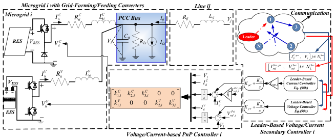
Figure 3: Electrical Scheme of MG $i$ with Leader-based Voltage/Current Distributed Secondary Controller.

6.1 Leader-based Voltage/Current Distributed Secondary Controller

The leader-based voltage and current distributed secondary controller is proposed in this subsection to achieve transfer reference information in a distributed way.

Based on (49) and (50), the transfer function from voltage reference $z_{ref_{[i]}}^{Pri,V}$ and current reference $z_{ref_{[i]}}^{Pri,C}$ to output voltage $V_{i}$ and output current $I_{ti}^{C}$ can be written as $\hat{H}_{i}(sI-\hat{F}_{i})\tilde{M}_{i}$ where $\tilde{M}_{i}$ collects the second and third columns of $\hat{M}_{i}$. If setting $s=0Hz$, the unit matrix is obtained which means the primary PnP controller can be approximated as unit-gain

$$V_{i} =V_{ref,i}^{Pri}$$ (97a)

$$\frac{I_{ti}^{C}}{I_{cap,i}} =I_{ti}^{C,pu}=I_{ref,i}^{Pri,pu}$$ (97b)

The secondary control layer exploit a communication network interconnecting MGs and fulfilling the following Assumption

Assumption 2.

The communication graph ${\mathcal{G}}^{Sec}=({\mathcal{D}},{\mathcal{E}}^{Sec})$ is connected and undirected implying that communication links within MG clusters are bidirectional. Over each communication link $(i,j)\in{\mathcal{E}}^{Sec}$, the pairs of variables $(I_{ti}^{C,pu},V_{i})$ and $(I_{tj}^{C,pu},V_{j})$ are transmitted. Furthermore, the graph ${\mathcal{G}}^{Sec}$ is endowed with an additional node termed the leader node, carrying the reference values $(I_{ref}^{Sec,pu},V_{ref}^{Sec})$ and connected to at least one node belongs to ${\mathcal{D}}$.

The proposed leader-based voltage and current distributed secondary controller can be written as

$$e_{Vi} =\sum\limits_{j\in{\mathcal{N}}_{i}^{Sec}}a_{ij}\left({V_{i}}-{V_{j}}\right)+g_{i}\left({V_{i}}-{V_{ref}^{Sec}}\right)$$ (98a)

$$e_{Ci} =\sum\limits_{j\in{\mathcal{N}}_{i}^{Sec}}a_{ij}\left({I_{i}}^{C,pu}-{I_{j}}^{C,pu}\right)+g_{i}\left({I_{i}}^{C,pu}-{I_{ref}^{Sec,pu}}\right)$$ (98b)

where ${\mathcal{N}}_{i}^{Sec}$ is the set of communication neighbors of MG $i$, $a_{ij}=1$ if MGs $i$ and $j$ can communicate with each other through a communication link, $g_{i}=1$ if MG $i$ can receive the reference values about voltage and per-unit current which means $i\in{\mathcal{N}}_{L}^{Sec}$ and ${\mathcal{N}}_{L}^{Sec}$ is the set for MG who can receive the reference values.

To be specific, the current reference value $I_{ref}^{Sec,pu}$ is a per-unit value considering the total load requirement and the total system capacity. If the per-unit values of all the output currents from MGs are equals to the reference value, it means that MGs within the cluster share the output current properly according to their own capacities.

In matrix form, (98) is given by the equations:

$$e_{V} =(L+G)(V-V_{ref}^{Sec}\boldsymbol{1_{N}})$$ (99a)

$$e_{C} =(L+G)(I_{t}^{C,pu}-I_{ref}^{Sec,pu}\boldsymbol{1_{N}})$$ (99b)

where $e_{V}=[\text{ }e_{V1}\text{ }e_{V2}\text{ }\dots\text{ }e_{VN}]^{T}$, $V=[\text{ }V_{1}\text{ }V_{2}\text{ }\dots\text{ }V_{N}]^{T}$,$I_{t}^{C,pu}=[\text{ }I_{t1}^{C,pu}\text{ }I_{t2}^{C,pu}\text{ }\dots\text{ }I_{tn}^{C,pu}]^{T}$, and $G$ is a diagonal matrix with diagonal entries equal to the gains $g_{i}$. Based on Assumption 2, $L$ is symmetric Laplacian matrix.

Then, the error $e_{Vi}$ and $e_{Ci}$ are filtered by PI controllers respectively. In order to provide the output $\Delta V_{i}$ and $\Delta I_{ti}^{C,pu}$ of the secondary controller layer, it can be written as

$$\Delta V =-K_{pV}e_{V}-\int{K_{iV}e_{V}}$$ (100a)

$$\Delta I_{t}^{C,pu} =-K_{pC}e_{C}-\int{K_{iC}e_{C}}$$ (100b)

where $\Delta V=[\text{ }\Delta V_{1}\text{ }\Delta V_{2}\text{ }\dots\text{ }\Delta V_{N}]^{T}$, $\Delta I_{t}^{C,pu}=[\text{ }\Delta I_{t1}^{C,pu}\text{ }\Delta I_{t2}^{C,pu}\text{ }\dots\text{ }\Delta I_{tn}^{C,pu}]^{T}$, in addition, $K_{pV}$ and $K_{iV}$ are proportional and integral coefficients of the leader-based voltage controller and $K_{pC}$ and $K_{iC}$ are proportional and integral coefficients of the leader-based current controller. All the coefficients are common to all MGs, thus these are scalar variables.

Remark 6.

Here, for the consensus-based algorithm, in the literature[23], consider only the integral controllers interfacing with the consensus algorithm and the primary control level. In this paper, PI controller is used in order to improve the convergence speed of the secondary controller.

The relationship between the primary PnP controller and the leader-based secondary controller are shown in Fig. 3. Exploiting the unit gain approximation of primary loops, one obtains that (97) is replaced by

$$V =V_{ref}^{Pri}+\Delta V$$ (101a)

$$I_{t}^{C,pu} =I_{ref}^{Pri,pu}+\Delta I_{t}^{C,pu}$$ (101b)

where $V_{ref}^{Pri}=[\text{ }V_{ref,1}^{Pri}\text{ }V_{ref,2}^{Pri}\text{ }\dots\text{ }V_{ref,n}^{Pri}]^{T}$, $I_{ref}^{Pri,pu}=[\text{ }I_{ref,1}^{Pri,pu}\text{ }I_{ref,2}^{Pri,pu}\text{ }\dots\text{ }I_{ref,n}^{Pri,pu}]^{T}$.

Focusing the time derivative of (101), we get

$$\dot{V} =-K_{iV}[I+K_{pV}(L+G)]^{-1}e_{V}$$ (102a)

$$\dot{I}_{t}^{C,pu} =-K_{iC}[I+K_{pC}(L+G)]^{-1}e_{C}$$ (102b)

6.2 Stability Analysis

The aim is to show that under the effect of secondary control layer, all PCC voltage converge to the leader value $V_{ref}^{Sec}$ and all the output current converge to the same per-unit value $I_{ref}^{Sec,pu}$.

Lemma 4.

Under Assumption 2, $L$ is symmetric Laplacian matrix, $G=diag{[g_{1},g_{2},\dots,g_{n}]}$ is diagonal matrix in which $g_{i}\geq 0$ and at least one $g_{i}>0$, then matrix $L+G$ is positive definite.

Proof.

As mentioned in $\mathbf{Notation}$ at the beginning of this technical report, each vector $x\in\mathbb{R}^{n}$ can always be written in a unique way as

$$x=\hat{x}+\bar{x}\text{ }\text{with }\hat{x}\in H^{1}\text{ and }\bar{x}\in H_{\perp}^{1}$$ (103)

Then, one has

$$x^{T}(L+G)x=\hat{x}^{T}L\hat{x}+x^{T}Gx$$ (104)

(104) is equivalent to the two following cases

$$\text{If }\hat{x}\neq 0\text{, }\underbrace{\hat{x}^{T}L\hat{x}}_{>0}+\underbrace{{x}^{T}G{x}}_{\geq 0} >0$$ (105a)

$$\text{If }\hat{x}=0\text{, }\underbrace{\bar{x}^{T}L\bar{x}}_{=0}+\underbrace{\bar{x}^{T}G\bar{x}}_{>0} >0$$ (105b)

Thus, matrix $L+G$ is positive definite matrix. ∎

Corollary 1.

Under Lemma 4, matrix $(L+G)^{-1}$ is positive definite and matrix $[I+\alpha(L+G)]^{-1}$ where scalar $\alpha>0$ is also positive definite.

We recall that if $\alpha$ is a scalar, $A$ is positive definite matrix and $I$ is unit matrix which is also positive definite matrix, from Woodbury matrix identity theory [24] , one has

$$[I+\alpha A]^{-1}=\alpha^{-1}A^{-1}-\alpha^{-1}A^{-1}(\alpha^{-1}A^{-1}+I)^{-1}\alpha^{-1}A^{-1}$$ (106)

Lemma 5.

[25] Let $A$, $B$ $\in\mathbb{R}^{n\times n}$ be positive definite matrices. If $AB=BA$ is satisfied, then $AB$ is positive definite.

Lemma 6.

Under Lemma 5 and Corollary 1 and eq. (106), it is known that scalar $K_{pV}>0$ and $(L+G)$ is positive definite matrix, matrix $(L+G)[I+K_{pV}(L+G)]^{-1}$ is positive definite.

Proof.

From Corollary 1, matrix $[I+K_{pV}(L+G)]^{-1}$ is positive. Then, from (106), one has

$$(L+G)[I+K_{pV}(L+G)]^{-1} =K_{pV}^{-1}I-\left(K_{pV}^{-1}\right)^{2}\left[K_{pV}^{-1}(L+G)^{-1}+I\right]^{-1}\left(L+G\right)^{-1}$$ (107)

$$=K_{pV}^{-1}I-\left(K_{pV}^{-1}\right)^{2}\left[K_{pV}^{-1}+(L+G)\right]^{-1}$$

Then

$${}^{-1}(L+G) =K_{pV}^{-1}I-\left(K_{pV}^{-1}\right)^{2}\left(L+G\right)^{-1}\left[K_{pV}^{-1}(L+G)^{-1}+I\right]^{-1}$$ (108)

$$=K_{pV}^{-1}I-\left(K_{pV}^{-1}\right)^{2}\left[K_{pV}^{-1}+(L+G)\right]^{-1}$$

Comparing (107) with (108), we have

$$(L+G)[I+K_{pV}(L+G)]^{-1}=[I+K_{pV}(L+G)]^{-1}(L+G)$$ (109)

To conclude, from Lemma 5, since both matrices $(L+G)$ and $[I+K_{pV}(L+G)]^{-1}$ are positive definite, combined with (109), the matrix $(L+G)[I+K_{pV}(L+G)]^{-1}$ is positive definite. ∎

Note that the consensus schemes (98a)-(100a) and (98b)-(100b) have the same structure. Then, in the following, we show convergence to the leader reference value only for voltages.

We consider the following candidate as Lyapunov function

$$Z=\frac{1}{2}e_{V}^{T}P^{Sec}e_{V},\text{ where }P^{Sec}>0$$ (110)

The time derivative of (110) is

$$\dot{Z} =e_{V}^{T}P^{Sec}(L+G)\dot{V}$$ (111)

$$=-K_{iV}e_{V}^{T}P^{Sec}(L+G)[I+K_{pV}(L+G)]^{-1}e_{V}$$

$$=\frac{-K_{iV}}{2}e_{V}^{T}[P^{Sec}O+O^{T}P^{Sec}]e_{V}$$

where $O=(L+G)[I+K_{pV}(L+G)]^{-1}$.

Based on Lemma 6, matrix $O$ is positive definite. Based on Lyapunov theory [26], there exists positive definite matrix $P^{Sec}$ which can make $P^{Sec}O+O^{T}P^{Sec}$ is positive definite. Therefore

$$\dot{Z}=\frac{-K_{iV}}{2}e_{V}^{T}[P^{Sec}O+O^{T}P^{Sec}]e_{V}<\frac{-K_{iV}}{2}\sigma_{min}(P^{Sec}O+O^{T}P^{Sec})||e_{V}||^{2}<0$$ (112)

where $\sigma_{min}(P^{Sec}O+O^{T}P^{Sec})$ denotes the minimal eigenvalues of the symmetric matrix $P^{Sec}O+O^{T}P^{Sec}$. From (112), one has that the tracking error $e_{V}$ goes to zero, and that all PCC voltages converge to the reference value provided by the leader. The convergence of output currents to the reference value is the same as above.

7 Hardware-in-Loop Tests

In order to verify the effectiveness of proposed primary PnP controller combined with leader-based voltage/current distributed controllers for MG clusters, real-time HiL tests are carried out based on dSPACE 1006. The real-time simulation model comprises four MGs with meshed electrical topology shown in Fig. 4. The capacity ratio for four MGs rated capacity is $1:2:3:4$ from MGs $1-4$. Communication network has the same topology of the electrical network. And MG $1$ is the only one receiving the leader information. The nominal voltage for the dc MG is 48V. In addition, in Appendix B, the electrical setup information is shown in TABLE 1, the transmission lines parameters are shown in TABLE 2 and the control coefficients are shown in TABLE 3.

Figure 4: System Configuration of Hardware-in-Loop Test.

7.1 Case 1: PnP Test considering Primary Control Level

In this subsection, the effectiveness of the proposed primary PnP controller is verified. Each MG is started separately. At the beginning, we set different voltage and current references for different MGs. At $t=T1$, MGs $1-3$ are connected together without changing the control coefficients. As shown in Fig. 5(a), after the connection of MGs $1-3$, only small disturbances exist in the voltage waveform. Moreover, there is no major disturbance affecting the output currents as shown in Fig. 5(b). Then at $t=T2$, MG $4$ is connected to the system. Similarly, as shown in Fig. 5, after small disturbance, both the output voltage and current track the respective reference values.

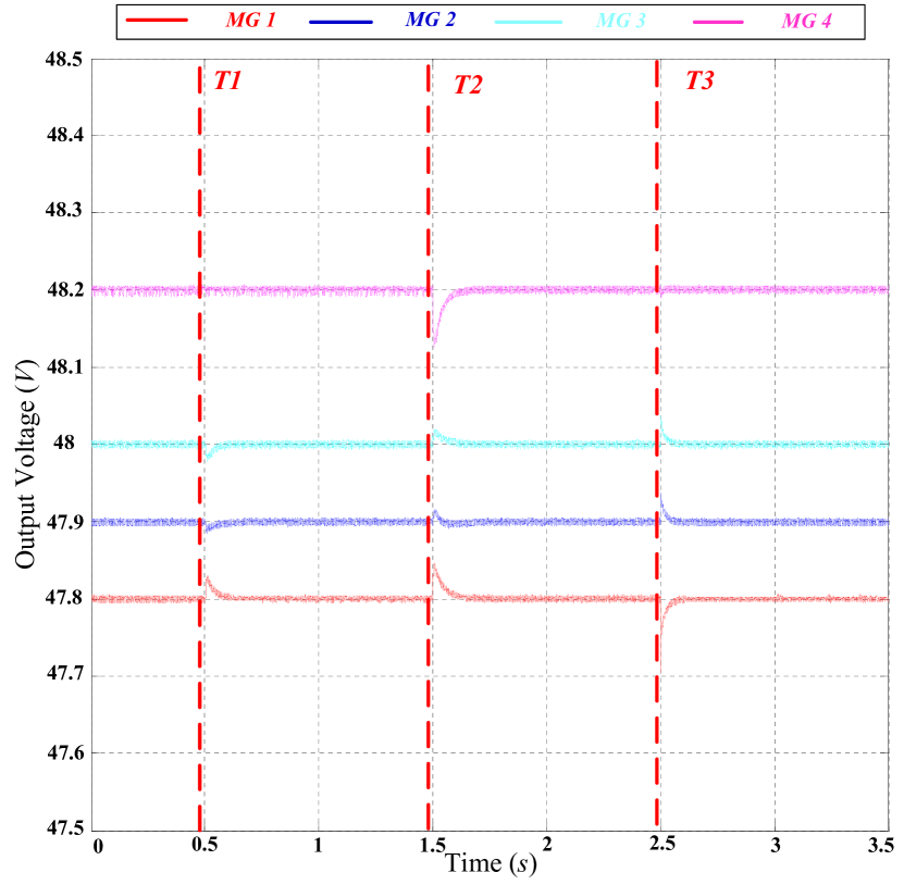
(a) Voltage Performance for PnP Test.

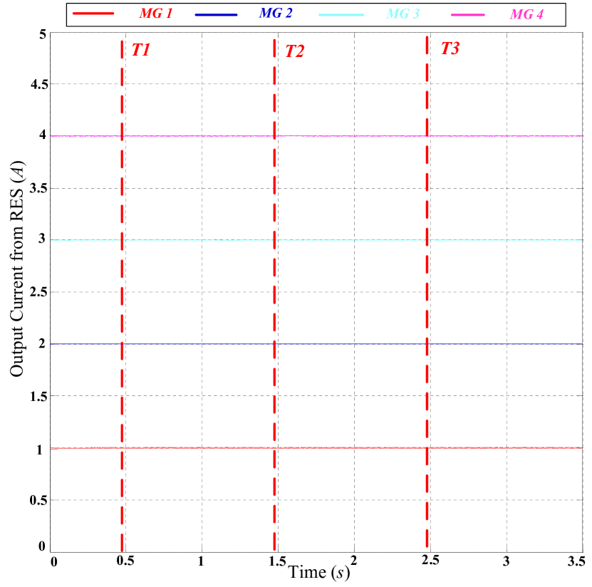
(b) Current Performance for PnP Test.

Figure 5: The Plug-in/-out Performance of primary PnP controllers.

Fig. 6 illustrates the current tracking performance by changing the current references for different modules. At $t=T1$, four MGs are connected together simultaneously. At $t=T2$, the current reference for MG $1$ is changed from $1A$ to $2.5A$. At $t=T3$, the current reference for MG $2$ is changed from $2A$ to $3.5A$. At $t=T4$, the current reference for MG $3$ is changed from $3A$ to $1.5A$. At $t=T5$, the current reference for MG $4$ is changed from $4A$ to $5.5A$. As shown in Fig. 6(b), whether the current references are increased or decreased, the output currents can track the changed reference. In addition, as shown in Fig. 6(a), when the current references are changed, the output voltages are only affected by little oscillations approximately $0.05V$.

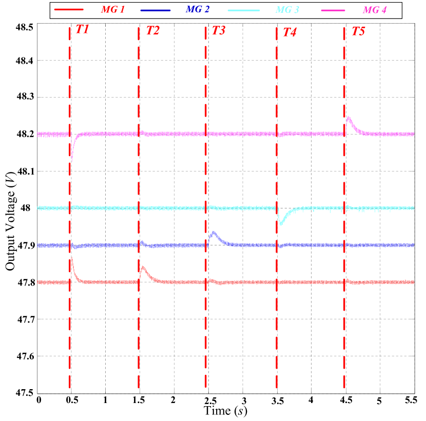
(a) Voltage Tracking Performance.

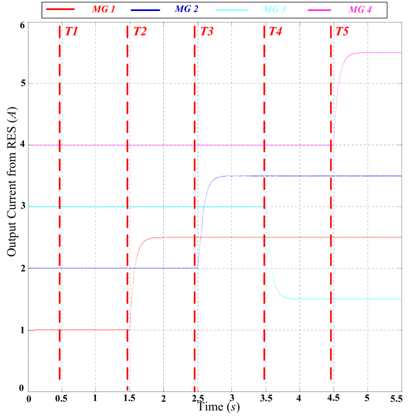
(b) Current Tracking Performance.

Figure 6: Voltage and Current Tracking Performance of PnP decentralized controllers

7.2 Case 2: Leader-Based Voltage/Current Distributed Secondary Controller Test

In this subsection, the effect of proposed leader-based voltage/current distributed secondary controller is verified. At $t=T1$, four MGs are connected together simultaneously. At $t=T2$, the proposed leader-based voltage controller is enabled and the leader value is set as $48V$. It is illustrated in Fig. 7(a) that after $t=T2$, the output voltages converge to the leader reference under $0.3s$. Then, at $t=T3$, the proposed leader-based current controller is enabled and leader value is set as $0.3p.u.$. As shown in Fig. 8(a), the proposed current controller can achieve current sharing in proportional and Fig. 8(b) illustrates that the per-unit current values can converge to the leader value within $1s$. In addition, Fig. 7(b) illustrates that only $0.04V$ oscillations exist in the output voltages when enabling the leader-based current controller. Furthermore, when the reference for leader-based voltage controller is changed from $48V$ to $49V$ at $t=T4$, the output voltage still track the leader reference, as shown in Fig. 7(a). Similarly, when the reference for leader-based current controller is changed from $0.3p.u.$ to $0.4p.u.$ at $t=T5$, the output current can also track the new value as shown in Fig. 8(b). Fig. 7(c) illustrates that when the reference for leader-based current is changed, the output voltages are not affected.

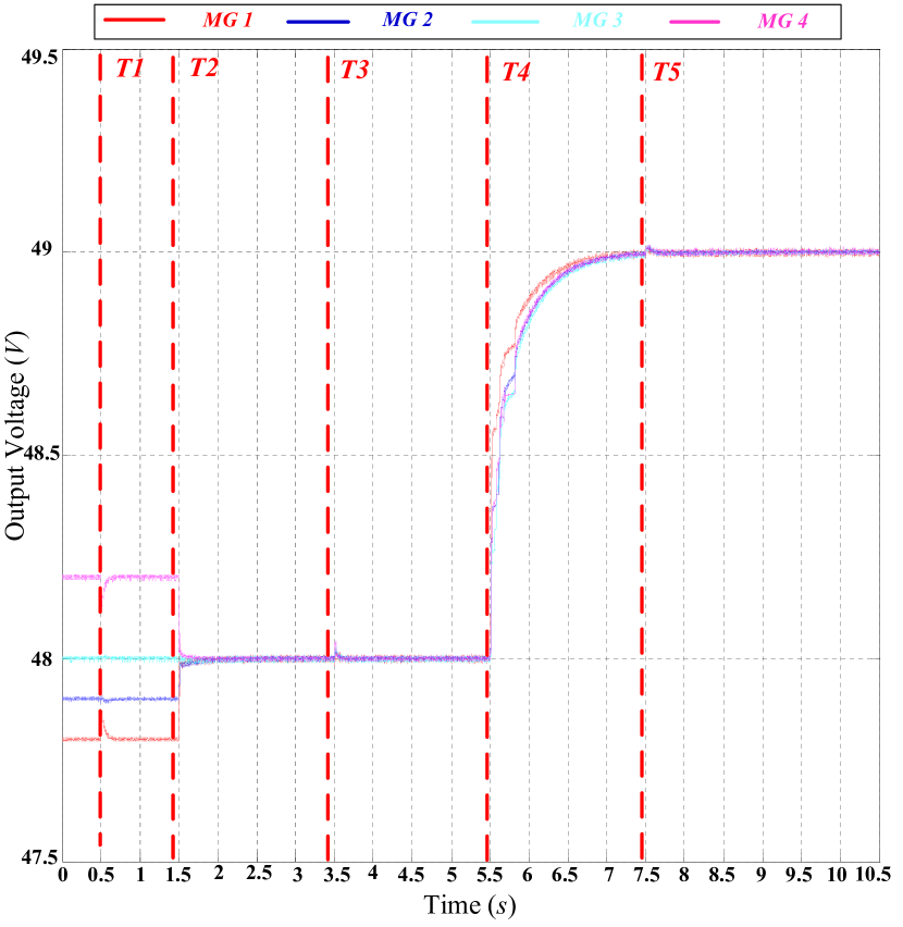
(a) Voltage Performance.

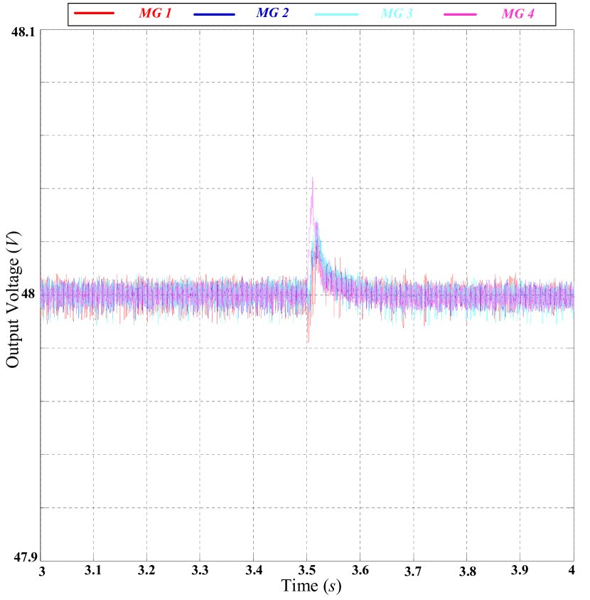
(b) Zoomed in Voltage Performance Between $3s$ and $4s$.

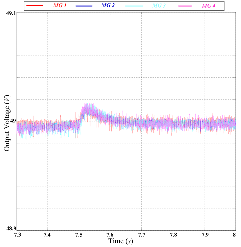
(c) Zoomed in Voltage Performance Between $7.3s$ and $8s$.

Figure 7: Voltage Performance for Leader-Based Voltage Secondary Controllers.

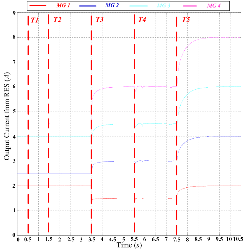
(a) Current Performance.

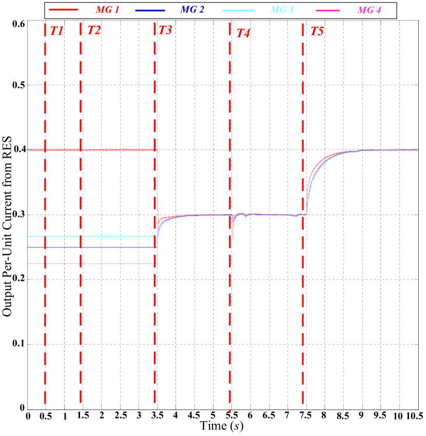
(b) Per-Unit Current Performance.

Figure 8: Current Performance for Leader-Based Current Secondary Controllers.

7.3 Case 3: PnP Test Considering Both Primary and Secondary Control Level

In this subsection, the PnP effect of both primary and secondary controllers is tested. At $t=T1$, four MFs are connected together simultaneously. At $t=T2$ and $T3$, the proposed leader-based voltage controller and leader-based current controller are enabled, respectively. At $t=T4$, MG $2$ is plugged out of the MG cluster which means the communication links and electrical lines are all disconnected with the MG cluster. As shown in Figs. 9 and 10, the other three MGs still operate in a stable way and then keep tracking the leader reference from the secondary control level. Meanwhile, MG $2$ can still use its own primary controller following the reference from the primary control level which are $47.8V$ for voltage and $0.25p.u.$ for current. At $t=T5$, MG $2$ is plugged into the cluster and the communication links of MG $2$ are also enabled. As shown in Fig. 9 and 10 after $t=T5$, both the output voltage and current of MG $2$ start to track the reference value of the leader node. Overall, the simulation results shows that even in presence of plug-in/out events, the MG cluster can behave in a stable way. And both output voltage and current tracking performance can be guaranteed. Furthermore, during the whole test, the control coefficients for each MG are not changed.

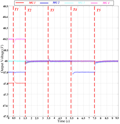
Figure 9: Voltage Performance for PnP Test considering both the Primary and Secondary Level.

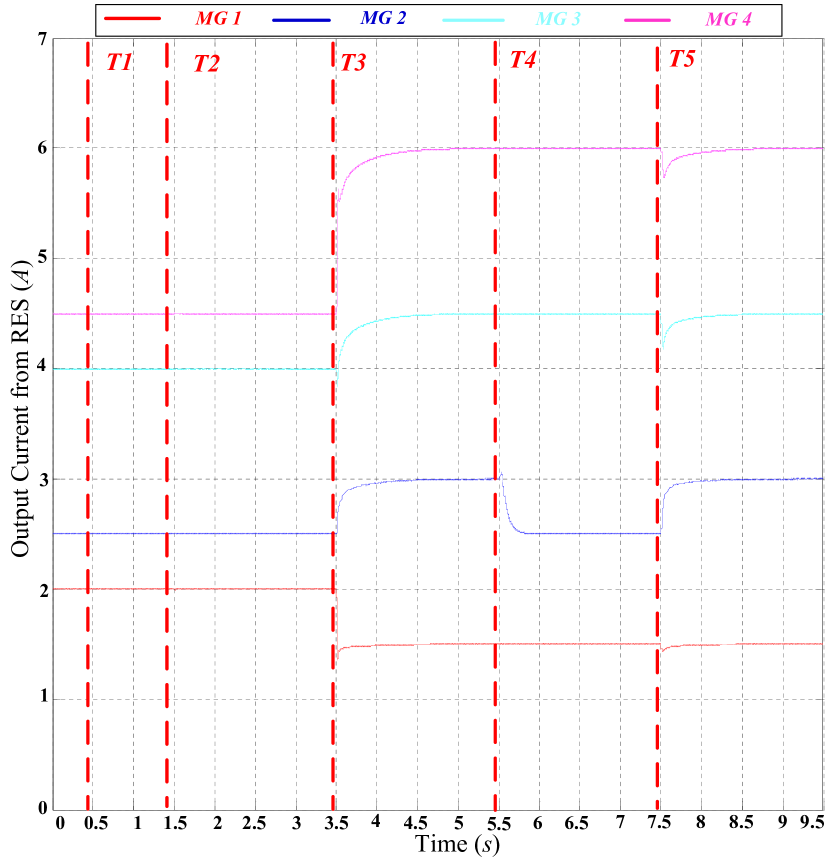
(a) Current Performance.

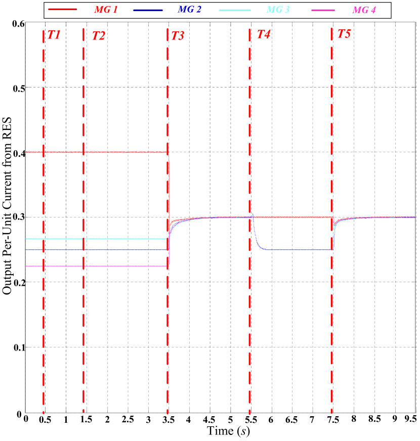
(b) Per-Unit Current Performance.

Figure 10: Current Performance for PnP Test considering both the Primary and Secondary Level.

8 Conclusions

In this paper, a hierarchical PnP Voltage/Current Controller for DC microgrid clusters with grid-forming/feeding modules is proposed including primary control level and secondary control level. In the primary control level, a novel PnP controller is proposed for a MG with grid-forming/feeding converters to achieve both the output voltages and currents tracking with the local control reference. A set only related to the local system information for control coefficients is found by which the controller can always be stable avoiding solving LMI problem. Meanwhile, the MG can achieve plug-in/out operation without changing the control coefficients to guarantee global stability of the MG cluster. In the secondary control level, the leader-based voltage/current distributed secondary controller is proposed to achieve both the voltage and current tracking with the information from the higher control level. Each MG only requires its own information and the information of its neighbours on the communication network graph. By approximating the primary PnP controller with unitary gains, the model of the whole system is established whose stability is proved by Lyapunov stability theory. Finally, the theoretical results are proven by the hardware in loop tests.

Appendix A Matrices appearing in microgrid models

A.1 Matrices in the model of CDGU

This appendix collects all matrices appearing in Section 2.

Overall model of a MG composed by $N$ CDGUs

$$\begin{bmatrix}{{\dot{x}}}_{[1]}^{C}\\ {{\dot{x}}}_{[2]}^{C}\\ {{\dot{x}}}_{[3]}^{C}\\ \vdots\\ {{\dot{x}}}_{[N]}^{C}\end{bmatrix} =\underbrace{\left[\begin{array}[]{ccccc}A_{11}^{C}+A_{load,1}^{C}&A_{12}^{C}&A_{13}^{C}&\dots&A_{1N}^{C}\\ A_{21}^{C}&A_{22}+A_{load,2}^{C}&A_{23}&\dots&A_{2N}^{C}\\ A_{31}^{C}&A_{32}^{C}&A_{33}+A_{load,3}^{C}&\dots&A_{3N}^{C}\\ \vdots&\vdots&\vdots&\ddots&\vdots\\ A_{N1}^{C}&A_{N2}^{C}&A_{N3}^{C}&\dots&A_{NN}+A_{load,N}^{C}\end{array}\right]}_{\mathbf{A^{C}}}\begin{bmatrix}{x}_{[1]}^{C}\\ {x}_{[2]}^{C}\\ {x}_{[3]}^{C}\\ \vdots\\ {x}_{[N]}^{C}\end{bmatrix}+$$ (113)

$$+\,\underbrace{\begin{bmatrix}B_{1}^{C}&0&\dots&0\\ 0&B_{2}^{C}&\ddots&\vdots\\ \vdots&\ddots&\ddots&0\\ 0&\dots&0&B_{N}^{C}\end{bmatrix}}_{\mathbf{B^{C}}}\begin{bmatrix}{u}_{[1]}^{C}\\ {u}_{[2]}^{C}\\ \vdots\\ {u}_{[N]}^{C}\end{bmatrix}+\underbrace{\begin{bmatrix}M_{1}^{C}&0&\dots&0\\ 0&M_{2}^{C}&\ddots&\vdots\\ \vdots&\ddots&\ddots&0\\ 0&\dots&0&M_{N}^{C}\end{bmatrix}}_{\mathbf{M^{C}}}\begin{bmatrix}{d}_{[1]}^{C}\\ {d}_{[2]}^{C}\\ \vdots\\ {d}_{[N]}^{C}\end{bmatrix}$$

$$\begin{bmatrix}{z}_{[1]}^{C}\\ {z}_{[2]}^{C}\\ {z}_{[3]}^{C}\\ \vdots\\ {z}_{[N]}^{C}\end{bmatrix} =\underbrace{\begin{bmatrix}H_{1}^{C}&0&0&\dots&0\\ 0&H_{2}^{C}&0&\ddots&\vdots\\ 0&0&H_{3}^{C}&\ddots&0\\ \vdots&\ddots&\ddots&\ddots&0\\ 0&\dots&0&0&H_{N}^{C}\end{bmatrix}}_{\mathbf{H^{C}}}\begin{bmatrix}{x}_{[1]}^{C}\\ {x}_{[2]}^{C}\\ {x}_{[3]}^{C}\\ \vdots\\ {x}_{[N]}^{C}\end{bmatrix}.$$

A.2 Matrices in the model of MG Clusters

This appendix provides all matrices appearing in Section 4.

Overall model of MG clusters composed by $N$ MGs

$$\begin{bmatrix}{{\dot{x}}}_{[1]}\\ {{\dot{x}}}_{[2]}\\ {{\dot{x}}}_{[3]}\\ \vdots\\ {{\dot{x}}}_{[N]}\end{bmatrix} =\underbrace{\left[\begin{array}[]{ccccc}A_{11}+A_{load,1}&A_{12}&A_{13}&\dots&A_{1N}\\ A_{21}&A_{22}+A_{load,2}&A_{23}&\dots&A_{2N}\\ A_{31}&A_{32}&A_{33}+A_{load,3}&\dots&A_{3N}\\ \vdots&\vdots&\vdots&\ddots&\vdots\\ A_{N1}&A_{N2}&A_{N3}&\dots&A_{NN}+A_{load,N}\end{array}\right]}_{\mathbf{A}}\begin{bmatrix}{x}_{[1]}\\ {x}_{[2]}\\ {x}_{[3]}\\ \vdots\\ {x}_{[N]}\end{bmatrix}+$$ (114)

$$+\,\underbrace{\begin{bmatrix}B_{1}&0&\dots&0\\ 0&B_{2}&\ddots&\vdots\\ \vdots&\ddots&\ddots&0\\ 0&\dots&0&B_{N}\end{bmatrix}}_{\mathbf{B}}\begin{bmatrix}{u}_{[1]}\\ {u}_{[2]}\\ \vdots\\ {u}_{[N]}\end{bmatrix}+\underbrace{\begin{bmatrix}M_{1}&0&\dots&0\\ 0&M_{2}&\ddots&\vdots\\ \vdots&\ddots&\ddots&0\\ 0&\dots&0&M_{N}\end{bmatrix}}_{\mathbf{M}}\begin{bmatrix}{d}_{[1]}\\ {d}_{[2]}\\ \vdots\\ {d}_{[N]}\end{bmatrix}$$

$$\begin{bmatrix}{z}_{[1]}\\ {z}_{[2]}\\ {z}_{[3]}\\ \vdots\\ {z}_{[N]}\end{bmatrix} =\underbrace{\begin{bmatrix}H_{1}&0&0&\dots&0\\ 0&H_{2}&0&\ddots&\vdots\\ 0&0&H_{3}&\ddots&0\\ \vdots&\ddots&\ddots&\ddots&0\\ 0&\dots&0&0&H_{N}\end{bmatrix}}_{\mathbf{H}}\begin{bmatrix}{x}_{[1]}\\ {x}_{[2]}\\ {x}_{[3]}\\ \vdots\\ {x}_{[N]}\end{bmatrix}.$$

Appendix B Electrical Parameters and Control Coefficients for HiL Test

In this appendix, all the electrical parameters and HiL control coefficients used in Section 7 are provided.

Table 1: Electrical setup parameters

Parameter	Symbol	Value
Output capacitance	$C_{t*}$	2.2 $mF$
Inductance for CDGU	$L_{t*}^{C}$	0.018$\mbox{ }H$
Inductor + switch loss resistance for CDGU	$R_{t*}^{C}$	0.2 $\Omega$
Inductance for VDGU	$L_{t*}^{V}$	0.0018$\mbox{ }H$
Inductor + switch loss resistance for VDGU	$R_{t*}^{V}$	0.1 $\Omega$
Switching frequency	$f_{sw}$	10 kHz

Table 2: Transmission lines parameters

Connected MGs $(i,j)$	Resistance $R_{i,j}(\Omega)$	Inductance $L_{i,j}(mH)$
$(1,2)$	0.3	1.8
$(2,3)$	0.6	5.4
$(3,4)$	0.8	7.2
$(4,1)$	0.7	3.6

Table 3: Control Coefficients

Control Coefficients		Symbol	Value
Primary Control Level for Single MG	Coefficients for CDGUs	$k_{1,*}^{C}$	-0.01
		$k_{2,*}^{C}$	-2.7015
		$k_{3,*}^{C}$	40.4018
	Coefficients for VDGUs	$k_{1,*}^{V}$	-0.480
		$k_{2,*}^{V}$	-0.108
		$k_{3,*}^{V}$	30.673
Secondary Control Level for MG Cluster	Leader-based Voltage Controllers	$k_{pV}$	4
		$k_{iV}$	22
	Leader-based Current Controllers	$k_{pC}$	3
		$k_{iC}$	20

References

• [1] J. M. Guerrero, J. C. Vasquez, J. Matas, D. Vicuna, L. García, and M. Castilla, “Hierarchical control of droop-controlled AC and DC microgrids - A general approach toward standardization,” IEEE Transactions on Industrial Electronics, vol. 58, no. 1, pp. 158–172, 2011.
• [2] R. Han, L. Meng, G. Ferrari-Trecate, E. A. A. Coelho, J. C. Vasquez, and J. M. Guerrero, “Containment and consensus-based distributed coordination control to achieve bounded voltage and precise reactive power sharing in islanded ac microgrids,” IEEE Transactions on Industry Applications, vol. PP, no. 99, pp. 1–1, 2017.
• [3] J. Rocabert, A. Luna, F. Blaabjerg, and P. Rodríguez, “Control of power converters in ac microgrids,” IEEE Transactions on Power Electronics, vol. 27, no. 11, pp. 4734–4749, Nov 2012.
• [4] T. Dragičević, X. Lu, J. Vasquez, and J. Guerrero, “DC microgrids–part I: A review of control strategies and stabilization techniques,” IEEE Transactions on Power Electronics, vol. 31, no. 7, pp. 4876–4891, 2016.
• [5] H. Wang, M. Han, R. Han, J. Guerrero, and J. Vasquez, “A decentralized current-sharing controller endows fast transient response to parallel dc-dc converters,” IEEE Transactions on Power Electronics, vol. PP, no. 99, pp. 1–1, 2017.
• [6] Q. Shafiee, T. Dragičević, J. C. Vasquez, and J. M. Guerrero, “Hierarchical Control for Multiple DC-Microgrids Clusters,” IEEE Transactions on Energy Conversion, vol. 29, no. 4, pp. 922–933, 2014.
• [7] V. Nasirian, S. Moayedi, A. Davoudi, and F. L. Lewis, “Distributed cooperative control of dc microgrids,” IEEE Transactions on Power Electronics, vol. 30, no. 4, pp. 2288–2303, April 2015.
• [8] S. Riverso, M. Farina, and G. Ferrari-Trecate, “Plug-and-Play Model Predictive Control based on robust control invariant sets,” Automatica, vol. 50, no. 8, pp. 2179–2186, 2014.
• [9] S. Bansal, M. Zeilinger, and C. Tomlin, “Plug-and-play model predictive control for electric vehicle charging and voltage control in smart grids,” in IEEE 53rd Conference on Decision and Control,, 2014, pp. 5894–5900.
• [10] M. Tucci, S. Riverso, J. C. Vasquez, J. M. Guerrero, and G. Ferrari-Trecate, “A decentralized scalable approach to voltage control of dc islanded microgrids,” IEEE Transactions on Control Systems Technology, vol. 24, no. 6, pp. 1965–1979, Nov 2016.
• [11] M. Tucci, S. Riverso, and G. Ferrari-Trecate, “Line-independent plug-and-play controllers for voltage stabilization in dc microgrids,” IEEE Transactions on Control Systems Technology, vol. PP, no. 99, pp. 1–9, 2017.
• [12] J. Zhao and F. Dörfler, “Distributed control and optimization in DC microgrids,” Automatica, vol. 61, pp. 18–26, 2015.
• [13] D. Wu, F. Tang, T. Dragicevic, J. M. Guerrero, and J. C. Vasquez, “Coordinated control based on bus-signaling and virtual inertia for islanded dc microgrids,” IEEE Transactions on Smart Grid, vol. 6, no. 6, pp. 2627–2638, Nov 2015.
• [14] X. Zhao, Y. W. Li, H. Tian, and X. Wu, “Energy management strategy of multiple supercapacitors in a dc microgrid using adaptive virtual impedance,” IEEE Journal of Emerging and Selected Topics in Power Electronics, vol. 4, no. 4, pp. 1174–1185, Dec 2016.
• [15] T. Dragicevic, J. M. Guerrero, J. C. Vasquez, and D. Skrlec, “Supervisory control of an adaptive-droop regulated DC microgrid with battery management capability,” IEEE Transactions on Power Electronics, vol. 29, no. 2, pp. 695–706, Feb 2014.
• [16] G. Ferrari-Trecate, A. Buffa, and M. Gati, “Analysis of coordination in multi-agent systems through partial difference equations,” IEEE Transactions on Automatic Control, vol. 51, no. 6, pp. 1058–1063, 2006.
• [17] F. M. Callier and C. A. Desoer, Linear system theory.   Springer Science & Business Media, 2012.
• [18] R. Han, L. Meng, J. M. Guerrero, and J. C. Vasquez, “Distributed nonlinear control with event-triggered communication to achieve current-sharing and voltage regulation in dc microgrids,” IEEE Transactions on Power Electronics, vol. PP, no. 99, pp. 1–1, 2017.
• [19] S. Skogestad and I. Postlethwaite, Multivariable feedback control: analysis and design.   New York, NY, USA: John Wiley & Sons, 1996.
• [20] R. Grone, R. Merris, and V. S. Sunder, “The Laplacian spectrum of a graph,” SIAM Journal on Matrix Analysis and Applications, vol. 11, no. 2, pp. 218–238, 1990.
• [21] C. Godsil and G. Royle, “Algebraic graph theory, volume 207 of graduate texts in mathematics,” 2001.
• [22] H. K. Khalil, Nonlinear systems (3rd edition).   Prentice Hall, 2001.
• [23] M. Tucci, L. Meng, J. M. Guerrero, and G. Ferrari-Trecate, “Consensus algorithms and plug-and-play control for current sharing in DC microgrids,” CoRR, vol. abs/1603.03624, 2016. [Online]. Available: http://arxiv.org/abs/1603.03624
• [24] N. Higham, Accuracy and Stability of Numerical Algorithms, 2nd ed.   Society for Industrial and Applied Mathematics, 2002. [Online]. Available: http://epubs.siam.org/doi/abs/10.1137/1.9780898718027
• [25] R. A. Horn and C. R. Johnson, Matrix analysis.   Cambridge university press, 2012.
• [26] Z. Qu, “Cooperative control of dynamical systems: applications to autonomous vehicles,” 2009.