Impulse-induced optimum control of chaos in dissipative driven systems

Abstract

Taming chaos arising from dissipative non-autonomous nonlinear systems by applying additional harmonic excitations is a reliable and widely used procedure nowadays. But the suppressory effectiveness of generic non-harmonic periodic excitations continues to be a significant challenge both to our theoretical understanding and in practical applications. Here we show how the effectiveness of generic suppressory excitations is optimally enhanced when the impulse transmitted by them (time integral over two consecutive zeros) is judiciously controlled in a not obvious way. This is demonstrated experimentally by means of an analog version of a universal model, and confirmed numerically by simulations of such a damped driven system including the presence of noise. Our theoretical analysis shows that the controlling effect of varying the impulse is due to a correlative variation of the energy transmitted by the suppressory excitation.

Obtaining full control of the chaotic dynamics of generic dissipative non-linear systems represents a fundamental interdisciplinary scientific and technological challenge. Among the different control procedures which have been proposed [1-3], the application of judiciously chosen periodic excitations [4-20] constitutes a reliable procedure in the context of dissipative non-autonomous systems. Hitherto, experimental control of chaos by periodic excitations has been demonstrated in many diverse systems, including laser systems [8,10,13,16], neurological systems [11], ferromagnetic systems [5], chemical reactions [17], and electronic systems [7,20]. It has been shown that the effectiveness of this non-feedback control procedure in non-autonomous systems depends critically upon the resonance condition and the initial phase difference between the primary (or chaos-inducing) periodic excitation and the secondary (or suppressory) periodic excitation, which has given rise to its denomination as phase control [19,20]. In such previous works, however, the flexibility of the control scenario against diversity in the suppressory excitations (SEs) was not studied since harmonic excitations have been overwhelmingly considered for the compelling reason of their simplicity. Clearly, the assumption of harmonic excitations means that the driving systems$-$whatever they might be$-$are effectively taken as linear. This mathematically convenient choice imposes a drastic and unnecessary restriction in the control scenario which is untenable for most natural and artificial systems due to their irreducible nonlinear nature [21]. Thus, to fully explore and exploit the physics of the control scenario, it seems appropriate to consider SEs exhibiting general features of periodic excitations which are the output of nonlinear systems, therefore being appropriately represented by Fourier series$-$not just by a single harmonic term. It has been shown, in particular, that the suppressory effectiveness of periodic excitations seems to be highly sensitive to their wave forms [2]. Since there are infinitely many different waveforms, an important question, both scientifically and technologically, is how can one explain in physical terms$-$providing in turn a quantitative characterization$-$the effect of the SE’s waveform on the control scenario.

Here, we experimentally demonstrate that a relevant quantity properly characterizing the effectiveness of generic SEs $f(t)$ having equidistant zeros in the control scenario is the impulse transmitted by the excitation over a half-period (hereafter referred to simply as the excitation’s impulse,

$$I\equiv\int_{0}^{T/2}f(t)dt,$$ (1)

with $T$ being the period)$-$ a quantity integrating the conjoint effects of the excitation’s amplitude, period, and waveform. The relevance of the excitation’s impulse has been observed previously in such different contexts as adiabatically ac-driven periodic Hamiltonian systems [22], chaotic dynamics of lasers [23], and discrete soliton ratchets [24], to cite just a few instances. For the sake of clarity, we consider an analog implementation of a simple universal model to discuss the impulse-induced chaos-control scenario: A damped-driven two-well Duffing oscillator described by the equation:

$$\overset{..}{x}=x-\beta\left[1+\eta f(t)\right]x^{3}-\delta\overset{.}{x}+\gamma\cos\left(\omega t\right),$$ (2)

where all the variables and parameters are dimensionless $\left(\beta,\eta,\delta,\gamma>0\right)$, while $f(t)$ is an unit-amplitude $T$-periodic excitation chosen to satisfy three remarkable properties. First, its waveform (and hence its impulse) is changed by solely varying a single parameter, the shape parameter $m$, between 0 and 1. Second, when $m=0$, then $f\left(t\right)_{m=0}=\sin\left(2\pi t/T+\varphi\right)$, with $\varphi$ being the initial phase difference between the two excitations involved for all values of the shape parameter, i.e., one recovers the standard case [20] of an harmonic excitation, while for the limiting value $m=1$ the excitation and its impulse vanish. And third, as a function of $m$, the SE’s impulse presents a single maximum at a certain value $m=m_{\max}^{impulse}$ (see Fig. 1 and [25] for the definition and additional properties of $f(t)$). Here, $\gamma\cos\left(\omega t\right)$ and $-\beta\eta x^{3}f\left(t\right)$ are to be regarded for convenience as the primary and suppressory excitations, respectively.

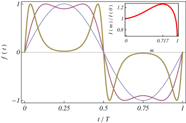
Figure 1: Suppressory $T$-periodic excitation $f(t)$ versus $t/T$ for three values of the shape parameter: $m=0$ (sinusoidal pulse, thin line), $m=0.717\simeq m_{\max}^{impulse}$ (nearly square-wave pulse, medium line), and $m=0.9999$ (double-humped pulse, thick line). The inset shows the corresponding normalized impulse $I(m)/I(m=0)$ versus $m$.

Also, we assume that, in the absence of any SE $\left(\eta=0\right)$, the Duffing oscillator (2) presents steady chaotic behavior which ultimately comes from a homoclinic bifurcation [26], while we will focus here on the effective case of the main resonance $\left(T=2\pi/\omega\right)$ between the two involved excitations in the presence of SEs $\left(\eta>0\right)$. As shown below, the simple and natural choice for $f(t)$ allows us to characterize experimentally the genuine effect on the chaos-control scenario of the impulse transmitted by generic SEs, as well as to explain theoretically that the controlling effect of varying the impulse is due to a correlative variation of the energy transmitted by the SE, allowing us to obtain useful analytical estimates of the chaotic threshold in the $\varphi-\eta$ control plane from Melnikov [26] and energy-based analyses, as is detailed in the Supplemental Material [25].

We investigated the impulse-induced chaos-control scenario in the laboratory by implementing an analog version of the Duffing oscillator (2) (see [25] for additional details). Our experimental results systematically indicate that complete regularization (i.e., periodic responses of any periodicity order) mainly appears inside two maximal islands in the $\varphi-\eta$ control plane which are roughly symmetric with respect to the two optimal suppressory values $\varphi_{opt}\equiv\left\{\pi/2,3\pi/2\right\}$, respectively, for all values of the shape parameter (see Fig. 2).

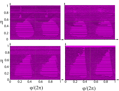
Figure 2: Experimentally obtained regions in the $\varphi-\eta$ control plane with $\varphi\in\left[0,2\pi\right]$ and $\eta\in\left[0,1\right]$ corresponding to chaos (non-uniform magenta regions), low-energy periodic orbits around some of the two fixed points $\left(x=\pm\beta^{-1/2},\overset{.}{x}=0\right)$ of the unperturbed Duffing oscillator (uniform light magenta regions), and higher-energy periodic orbits encircling both fixed points (uniform dark magenta regions) for four values of the shape parameter: (a) $m=0$, (b) $m=0.717\simeq m_{\max}^{impulse}$, (c) $m=0.9$, and (d) $m=0.95$. Fixed parameters: $\delta=0.25,\gamma=0.29,\beta=1,\omega=1$.

The analysis of the experimental data gives rise to the following genuine features of the present chaos-control scenario. While both the size and the form of the boundaries of the maximal regularization islands vary as the SE’s impulse changes by solely varying $m$, they remain roughly centered around the optimal values $\varphi_{opt}\equiv\left\{\pi/2,3\pi/2\right\}$ (note that the entire diagrams of Fig. 2 are periodic along the $\varphi$-axis, with fundamental period equal to $\pi$), confirming thus the theoretical predictions from Melnikov and energy-based analyses [25].

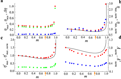
Figure 3: Experimental values of threshold amplitudes and regularization area in the control parameter plane versus shape parameter: (a) Lower threshold amplitude $\eta_{\min}$ (circles), upper threshold amplitude $\eta_{\max}$ (squares), and difference $\Delta\eta\equiv\eta_{\max}-\eta_{\min}$ (triangles) versus shape parameter $m$. (b) Normalized lower threshold amplitude $\eta_{\min,norm}=\eta_{\min,norm}\left(m\right)\equiv\eta_{\min}(m)/\eta_{\min}(m=0)$ (circles), normalized upper threshold amplitude $\eta_{\max,norm}=\eta_{\max,norm}(m)\equiv\eta_{\max}(m)/\eta_{\max}(m=0)$ (squares), and inverse of the normalized impulse $\left[I(m)/I(m=0)\right]^{-1}$ (solid line; cf. Eq. (S3) in Supplemental Material [25]). (c) Threshold amplitude $\eta_{\max}^{\prime}$ leading the Duffing oscillator to small-amplitude periodic oscillations around one of the fixed points $\left(x=\pm\beta^{-1/2},\overset{.}{x}=0\right)$ of the unperturbed Duffing oscillator (squares), its normalized version $\eta_{\max,norm}^{\prime}=\eta_{\max,norm}^{\prime}(m)\equiv\eta_{\max}^{\prime}(m)/\eta_{\max}^{\prime}(m=0)$ (circles), and analytical estimate of the latter [solid line; cf. Eq. (3)]. (d) Normalized areas of regularized regions in the $\varphi-\eta$ control plane, $A_{norm}=A_{norm}(m)\equiv A(m)/A\left(m=0\right)$ (squares), $A_{norm}^{\prime}=A_{norm}^{\prime}\left(m\right)\equiv A(m)/A_{total}$ (circles), in which $A(m)$ and $A_{total}$ are the regularization area and the total area, respectively. The solid line denotes the inverse of the normalized impulse $\left[I(m)/I(m=0)\right]^{-1}$, whereas the orange arrows indicate the value $m=m_{\max}^{impulse}\simeq 0.717$, i.e., the $m$ value at which the SE’s impulse is maximum. Fixed parameters: $\delta=0.25,\gamma=0.29,\beta=1,\omega=1$.

The lower, $\eta_{\min}$, and upper, $\eta_{\max}$, threshold values of the SE’s amplitude measured at the optimal suppressory values $\varphi=\varphi_{opt}\equiv\left\{\pi/2,3\pi/2\right\}$ as well as the difference $\Delta\eta\equiv\eta_{\max}-\eta_{\min}$ present, as functions of the shape parameter, a behavior quite similar to that of the inverse of the SE’ impulse [see Fig. 3(a)]. This can be seen more clearly in Fig. 3(b) in which it is shown the normalized amplitude thresholds $\eta_{\max}(m)/\eta_{\max}(m=0)$, $\eta_{\min}(m)/\eta_{\min}(m=0)$ together with the inverse of the normalized impulse $\left[I(m)/I(m=0)\right]^{-1}$ for the sake of comparison (see Supplemental Material [25]). In particular, we can see that the respective minima occur at values of the shape parameter which are very close in the sense that the difference between the corresponding values of the SE’s impulse is hardly noticeable.

Although we have not gotten a definitive explanation of the apparently anomalous behavior of $\eta_{\min}$ over a certain range of small values of $m$, it seems to be originated in the fractal character of the boundary for chaos in parameter space [27] together with the fact that over such a range of $m$ values the changes of the SE’s impulse are hardly noticeable [25]. The experimental results shown in Fig. 3(a) indicate that ever lower amplitudes $\eta_{\min}$ can suppress chaos as the impulse transmitted by the SE approaches its maximum value, whereas the corresponding suppressory ranges $\Delta\eta$ also decrease in the same way as $\eta_{\min}$ owing to the impulse-induced enhancement of the chaos-inducing effectiveness of the SE. This dependence of $\eta_{\min},\eta_{\max},\Delta\eta$ on the SE’s impulse, which is theoretically anticipated from Melnikov analysis [25], represents an essential feature of the present chaos-control scenario which is expected to be independent of the particular choice for the SE.

The lower values of the SE’s amplitude which suppress chaos by leading the Duffing oscillator to small-amplitude periodic oscillations around one of the fixed points $\left(x=\pm\beta^{-1/2},\overset{.}{x}=0\right)$ of the unperturbed Duffing oscillator $\left(\delta=\gamma=\eta=0\right)$, $\eta_{\max}^{\prime}$, present, as a function of the shape parameter, a behavior quite similar to that of the inverse of the SE’s impulse [see Fig. 3(c)]. Remarkably, we can see in Fig. 3(c) that the theoretical estimate of its normalized version,

$$\frac{\eta_{\max}^{\prime}(m)}{\eta_{\max}^{\prime}(m=0)}=\left[\frac{I(m)}{I(m=0)}\right]^{-1},$$ (3)

fits quite well the corresponding experimental values. Since the energy-based analysis giving rise to Eq. (3) is general in the sense that it can be applied to damped-driven systems of type (1) with generic (analytical) potentials $U(x)$ (see Supplemental Material [25]), one may expect that the dependence of $\eta_{\max}^{\prime}$ on the SE’s impulse represents an additional universal feature of the present chaos-control scenario.

The total area of regularized regions (i.e., those associated with periodic responses of any periodicity order), $A$, in the $\varphi-\eta$ control plane presents, as a function of the shape parameter, a behavior which exhibits relevant features that are common to those of the inverse of the SE’s impulse. Specifically, Fig. 3(d) shows that its normalized versions $A_{norm}\equiv A(m)/A\left(m=0\right)$ and $A_{norm}^{\prime}\equiv A(m)/A_{total}$ present a single minimum just at $m=m_{\max}^{impulse}\simeq 0.717$, i.e., the $m$ value at which the SE’s impulse is maximum (see Fig. 1). It is worth noting that the same behavior is theoretically anticipated for the area of the aforementioned maximal islands from the application of the Melnikov analysis to the crudest approximation of the SE $f(t)$, i.e., when solely the main harmonic of its Fourier expansion is retained (see Supplemental Material [25] for an analytical estimate of the maximal islands’ area). This inverse dependence of the regularization areas in the $\varphi-\eta$ control plane on the SE’s impulse represents an additional essential feature of the present chaos-control scenario which is expected to be especially useful in technological applications owing to it provides an universal criterion to guide the design of optimal SEs.

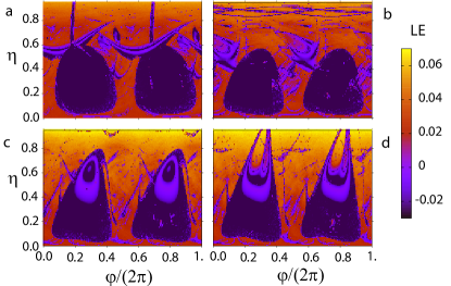
Figure 4: Numerically calculated maximal Lyapunov exponent in the $\varphi-\eta$ control plane for four values of the shape parameter: (a) $m=0$, (b) $m=0.717\simeq m_{\max}^{impulse}$ (i.e., the $m$ value at which the SE’s impulse is maximum), (c) $m=0.9$, and (d) $m=0.95$. Fixed parameters: $\delta=0.25,\gamma=0.29,\beta=1,\omega=1$.

Extensive computer simulations of Eq. (1) yielded numerical results from which we constructed three complementary types of diagrams providing useful information on both regularization regions in the $\varphi-\eta$ control plane and the nature of the regularized (periodic) responses: maximal Lyapunov exponent, period-distribution, and isospike diagrams (see Supplemental Material [25]). The conclusions arising from the analysis of these diagrams systematically agree with all the aforementioned experimental features of the present chaos-control scenario, as can be appreciated by comparing the maximal Lyapunov exponent diagrams shown in Fig. 4 with the respective experimental diagrams shown in Fig. 3.

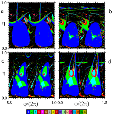
Figure 5: Numerically calculated regularization regions according to the waveform complexity (number of spikes or local maxima per period) of their solutions and chaotic regions (black) in the $\varphi-\eta$ control plane for four values of the shape parameter: (a) $m=0$, (b) $m=0.717\simeq m_{\max}^{impulse}$ (i.e., the $m$ value at which the SE’s impulse is maximum), (c) $m=0.9$, and (d) $m=0.95$. Fixed parameters: $\delta=0.25,\gamma=0.29,\beta=1,\omega=1$.

Regarding the nature of the regularized responses, the period-distribution and isospike diagrams inform us of the existence of a wide spectrum of periodic responses in different regions of the $\varphi-\eta$ control plane, the period-1 solutions being the prevailing responses over the two maximal regularization islands irrespective of the values of the SE’s impulse (see Figs. 5 and 6).

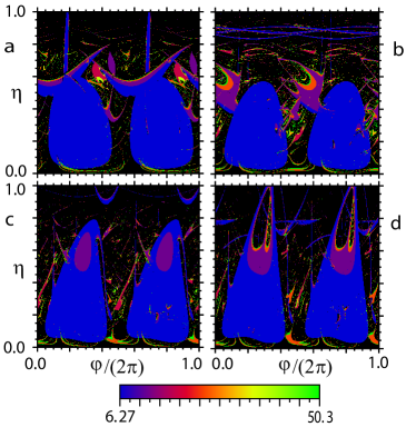
Figure 6: Numerically calculated regularization regions according to the period of their periodic solutions and chaotic regions (black) in the $\varphi-\eta$ control plane for four values of the shape parameter: (a) $m=0$, (b) $m=0.717\simeq m_{\max}^{impulse}$ (i.e., the $m$ value at which the SE’s impulse is maximum), (c) $m=0.9$, and (d) $m=0.95$. Fixed parameters: $\delta=0.25,\gamma=0.29,\beta=1,\omega=1$.

Importantly, our numerical results show that the present chaos-control scenario is robust against the presence of moderate-intensity Gaussian noise, with the two maximal regularization islands being the robustest regularization regions, which represents an invaluable feature due to the unavoidable presence of thermal noise in many physical contexts, including for instance many nanoscale devices. Specific examples are shown in [25].

During the last three decades or so [1-3], and on the basis of an overwhelming use of harmonic SEs, the effectiveness of this particular type of SE has been systematically explored in a vast diversity of physical contexts by independently varying its amplitude and frequency as control parameters. However, by taking into account the irreducible nonlinear nature of real-world periodic excitations, the present results demonstrate that the SE’s impulse is the relevant quantity providing a complete characterization of the suppressory effectiveness of generic SEs by means of an exquisite control of the injection of energy into a chaotic damped-driven system. Future work may extend the present impulse-induced chaos-control scenario to the control of diverse quantum phenomena associated with the so-called quantum chaos, such as dynamical localization [28] and quantum entanglement in systems in contact with environment [29].

Supplemental Material: Impulse-induced optimum control of chaos in dissipative driven systems

I Theoretical methods

I.1 Fourier expansion of the suppressory excitation (SE)

In our study we consider the elliptic SE

$$f(t)\equiv N\operatorname*{sn}\left(4Kt/T+\Phi\right)\operatorname*{dn}\left(4Kt/T+\Phi\right),$$ (S1)

in which $\operatorname*{sn}\left(\cdot\right)\equiv\operatorname*{sn}\left(\cdot;m\right)$ and $\operatorname*{dn}\left(\cdot\right)\equiv\operatorname*{dn}\left(\cdot;m\right)$ are Jacobian elliptic functions of parameter $m$ ($K\equiv K(m)$ is the complete elliptic integral of the first kind) S_1 , $\Phi=\Phi\left(m,\varphi\right)\equiv 2K(m)\varphi/\pi$, $\varphi\in\left[0,2\pi\right]$, $T\equiv 2\pi/\omega$, and

$$N=N(m)\equiv\left[a+b\left(1+\exp\left\{\frac{m-c}{d}\right\}\right)^{-1}\right]^{-1},$$ (S2)

is a normalization function ($a\equiv 0.43932,b\equiv 0.69796,c\equiv 0.3727,d\equiv 0.26883$) which is introduced for the elliptic excitation to have the same amplitude, 1, and period $T$, for any waveform (i.e., $\forall m\in\left[0,1\right]$). When $m=0$, then $f\left(t\right)_{m=0}=\sin\left(2\pi t/T+\varphi\right)$, i.e., one recovers the standard case of an harmonic SE, while for the limiting value $m=1$ the excitation vanishes. The effect of renormalization of the elliptic arguments is clear: with $T$ constant, solely the excitation’s impulse is varied by increasing the shape parameter $m$ from $0$ to $1$. Note that, as a function of $m$, the SE’s impulse per unit of amplitude and unit of period

$$I=I(m)\equiv\frac{N\left(m\right)}{2K\left(m\right)}$$ (S3)

presents a single maximum at $m=m_{\max}^{impulse}\simeq 0.717$ (see Fig. 1 of the main text).

The Fourier expansion of the elliptic SE (Eq. S1) reads

$$f(t) =\sum_{n=0}^{\infty}a_{n}(m)\sin\left[\left(2n+1\right)\left(\frac{2\pi t}{T}+\varphi\right)\right],$$ (S4)

$$a_{n}(m) \equiv\frac{\pi^{2}N(m)(n+\frac{1}{2})}{\sqrt{m}K^{2}(m)}\operatorname{sech}\left[\frac{(n+\frac{1}{2})\pi K(1-m)}{K(m)}\right],$$ (S5)

in which its Fourier coefficients satisfy the properties: i) $\lim_{m\rightarrow 1}a_{n}(m)=0$, ii) $a_{n}(m)$ exhibits a single maximum at $m=m_{\max}\left(n\right)$ such that $m_{\max}\left(n+1\right)>m_{\max}\left(n\right)$, $n=0,1,...$, iii) the normalized functions $a_{0}(m)/a_{0}(m=0)$ and $I(m,T)/I(m=0,T)\equiv\pi N(m)/(2K(m))$ present, as functions of $m$, similar behaviours while their maxima verify that $m_{\max}\left(n=0\right)\simeq 0.65$ is very close to $m_{\max}^{impulse}\simeq 0.717$ (see Fig. S1), and iv) the Fourier expansion (Eq. S4) is rapidly convergent over a wide range of values of the shape parameter. The following remarks may now be in order.

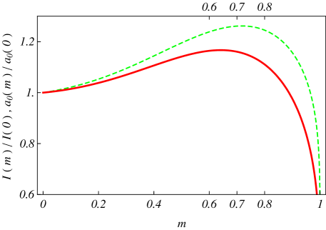
Figure S1: Comparison between the SE’s impulse and its first Fourier coefficient as functions of the shape parameter. Normalized first Fourier coefficient $a_{0}(m)/a_{0}(m=0)$ (Eq. S5, solid line) and SE’s impulse $I(m)/I(m=0)\equiv\pi N(m)/(2K(m))$ (Eq. S3, dashed line) versus shape parameter $m$. We can see that the respective single maxima occur at very close values of the shape parameter: $m_{\max}\left(n=0\right)\simeq 0.642$ and $m_{\max}^{impulse}\simeq 0.717$, respectively.

First, regarding analytical estimates, the property (iii) is relevant in the sense that it allows us to obtain an useful effective estimate of the chaotic threshold in the $\varphi-\eta$ control plane from Melnikov analysis (MA) S_2 ; S_3 by solely retaining the first harmonic of the Fourier expansion (Eq. S4):

$$f(t)\approx a_{0}(m)\sin\left(\omega t+\varphi\right).$$ (S6)

Second, regarding experiments, the property (iv) is relevant in the sense that it allows us to effectively approximate the elliptic SE by solely retaining the first two harmonics of its Fourier expansion over the range of values of the shape parameter of our interest ($0\leqslant m\lesssim 0.95$; see Fig. S2):

$$f(t;T,m,\varphi)\approx a_{0}(m)\sin\left(\omega t+\varphi\right)+a_{1}(m)\sin\left(3\omega t+3\varphi\right).$$ (S7)

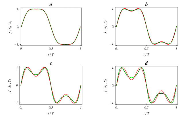
Figure S2: Comparison between the elliptic SE and its two- and three-harmonics approximations over a period for four values of the shape parameter. Plots of the elliptic SE (Eq. S1, dashed line), its two-harmonics approximation $S_{2}(t)\equiv a_{0}(m)\sin\left(\omega t+\varphi\right)+a_{1}(m)\sin\left(3\omega t+3\varphi\right)$ (cf. Eqs. S4 and S5, solid line), and its three-harmonics approximation $S_{3}(t)\equiv a_{0}(m)\sin\left(\omega t+\varphi\right)+a_{1}(m)\sin\left(3\omega t+3\varphi\right)+a_{2}(m)\sin\left(5\omega t+5\varphi\right)$ (cf. Eqs. S4 and S5, thin solid line ) versus time for four values of the shape parameter: a, $m=0.5$; b, $m=0.717\simeq m_{\max}^{impulse}$; c, $m=0.9$; d, $m=0.95$.

Third, regarding numerical simulations, we considered the entire Fourier expansion of the elliptic SE in order to obtain useful information concerning the effectiveness of the approximations used in the theoretical analysis and experiments (cf. Eqs. S6 and S7, respectively).

I.2 Chaotic threshold from Melnikov analysis

Melnikov introduced a function (now known as the Melnikov function (MF), $M\left(t_{0}\right)$) which measures the distance between the perturbed stable and unstable manifolds in the Poincaré section at $t_{0}$. If the MF presents a simple zero, the manifolds intersect transversally and chaotic instabilities result. See Refs.S_2 ; S_3 for more details about MA. Regarding Eq. (2) in the main text, note that keeping with the assumption of the MA, it is assumed that one can write $\delta=\varepsilon\overline{\delta},\gamma=\varepsilon\overline{\gamma},\eta=\varepsilon\overset{\_}{\eta}$ where $0<\varepsilon\ll 1$ while $\overset{\_}{\delta},\overline{\gamma},\overset{\_}{\eta},\beta,\omega$ are of order one. Thus, the application of MA to Eq. (2) in the main text yields the MF

$$M^{\pm}\left(t_{0}\right) =-D\pm A\sin\left(\omega t_{0}\right)+\frac{\pi\eta}{6\beta}\sum_{p=0}^{\infty}a_{p}\left(m\right)b_{p}\left(T\right)\cos\left[\Omega_{p}\left(T\right)t_{0}+\left(2p+1\right)\varphi\right],$$ (S8)

$$D \equiv\frac{4\delta}{3\beta},$$ (S9)

$$A \equiv\sqrt{\frac{2}{\beta}}\pi\gamma\omega\operatorname{sech}\left(\pi\omega/2\right),$$ (S10)

$$\Omega_{p}\left(T\right) \equiv\left(2p+1\right)\frac{2\pi}{T},$$ (S11)

$$b_{p}\left(T\right) \equiv\Omega_{p}^{2}\left(4+\Omega_{p}^{2}\right)\operatorname{csch}\left(\frac{\pi\Omega_{p}}{2}\right),$$ (S12)

where the coefficients $a_{p}\left(m\right)$ are given by Eq. S5, and where the positive (negative) sign refers to the right (left) homoclinic orbit of the underlying conservative Duffing oscillator $\left(\delta=\eta=\gamma=0\right)$:

$$x_{0,\pm}\left(t\right) =\pm\sqrt{\frac{2}{\beta}}\operatorname{sech}\left(t\right),$$ (S13)

$$\overset{.}{x}_{0,\pm}\left(t\right) =\mp\sqrt{\frac{2}{\beta}}\operatorname{sech}\left(t\right)\tanh\left(t\right).$$ (S14)

Let us assume that, in the absence of any SE $\left(\eta=0\right)$, the damped driven two-well Duffing oscillator (Eq. 2 in the main text) presents chaotic behaviour for which the respective MF,

$$M_{0}^{\pm}\left(t_{0}\right)\equiv-D\pm A\sin\left(\omega t_{0}\right),$$ (S15)

has simple zeros, i.e., $D\leqslant A$ or

$$\gamma\geqslant\gamma_{th}\equiv\frac{2\sqrt{2}\delta\cosh\left(\pi\omega/2\right)}{3\pi\sqrt{\beta}\omega},$$ (S16)

where the equal sign corresponds to the case of tangency between the stable and unstable manifolds S_3 . If we now let the SE act on the Duffing oscillator such that $B^{\ast}\leqslant A-D$, with

$$B^{\ast}\equiv\max_{t_{0}}\left\{\frac{\pi\eta}{6\beta}\sum_{p=0}^{\infty}a_{p}\left(m\right)b_{p}\left(T\right)\cos\left[\Omega_{p}t_{0}+\left(2p+1\right)\varphi\right]\right\},$$ (S17)

then this relationship represents a sufficient condition for $M^{\pm}\left(t_{0}\right)$ to change sign at some $t_{0}$. Thus, a necessary condition for $M^{\pm}\left(t_{0}\right)$ to always have the same sign is

$$B^{\ast}>A-D\equiv B_{\min}.$$ (S18)

Since $a_{p}\left(m\right)>0,b_{p}\left(T\right)>0,p=0,1,2,...$, one straightforwardly obtains

$$B^{\ast}\leqslant\frac{\pi\eta}{6\beta}\sum_{p=0}^{\infty}a_{p}\left(m\right)b_{p}\left(T\right),$$ (S19)

and hence,

$$\eta >\eta_{\min}\equiv\left(1-\frac{D}{A}\right)R,$$ (S20)

$$R \equiv\frac{6\beta A}{\pi\sum_{p=0}^{\infty}a_{p}\left(m\right)b_{p}\left(T\right)}.$$ (S21)

Note that Eq. S20 provides a lower threshold for the amplitude of the SE. Similarly, an upper threshold is obtained by imposing the condition that the SE may not enhance the initial chaotic state (i.e., it does not increase the (initial) gap from the homoclinic tangency condition),

$$B^{\ast}\leqslant\frac{\pi\eta}{6\beta}\sum_{p=0}^{\infty}a_{p}\left(m\right)b_{p}\left(T\right)<A+D\equiv B_{\max},$$ (S22)

and hence,

$$\eta<\eta_{\max}\equiv\left(1+\frac{D}{A}\right)R,$$ (S23)

which is a necessary condition for $M^{\pm}\left(t_{0}\right)$ to always have the same sign. Thus, the suitable (suppressory) amplitudes of the SE must satisfy

$$\eta_{\min}<\eta<\eta_{\max},$$ (S24)

while the width of the range of suitable amplitudes reads

$$\Delta\eta\equiv\eta_{\max}-\eta_{\min}=\frac{16\delta}{\pi\sum_{p=0}^{\infty}a_{p}\left(m\right)b_{p}\left(T\right)}.$$ (S25)

Figures S3 and S4 show how both the width of the range of suitable amplitudes $\Delta\eta$ (Eq. S25) and the threshold amplitudes $\eta_{\min},\eta_{\max}$ present a single minimum at $m=m_{\min}$ as the shape parameter $m$ is increased from 0 to 1 due to the dependence of the function $R$ on the shape parameter. While this minimum $m_{\min}\equiv m_{\min}(T)$ is very near $m_{\max}^{impulse}\simeq 0.717$ over a wide range of periods, one cannot expect an exact agreement between $m_{\min}$ and $m_{\max}^{impulse}$ for all periods owing to the dependence of the chaotic threshold on the common excitation period (main resonance). This means that ever lower amplitudes $\eta_{\min}$ can suppress chaos as the impulse transmitted by the SE approaches its maximum value, whereas the corresponding suppressory ranges $\Delta\eta$ also decrease in the same way as $\eta_{\min}$ owing to the impulse-induced enhancement of the chaos-inducing effectiveness of the SE. This dependence of $\eta_{\max},\eta_{\min},\Delta\eta$ on the SE’s impulse represents a genuine feature of the impulse-induced chaos-control scenario.

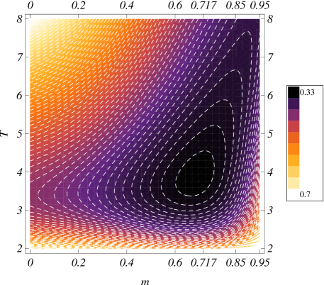
Figure S3: Width of the range of suitable suppressory amplitudes in the $m-T$ control plane. Contour plot of the function $\Delta\eta\equiv\eta_{\max}-\eta_{\min}$ (Eq. S24) versus shape parameter $m$ and period $T$. Note the existence of an absolute minimum at $m\simeq m_{\max}^{impulse},T\simeq 4$. System parameters: $\gamma=0.29,\delta=0.25,\beta=1.$

Figure S4: Threshold amplitudes and width of the range of suitable suppressory amplitudes versus shape parameter. Upper threshold amplitude $\eta_{\max}$ (Eq. S22, dotted line), lower threshold amplitude $\eta_{\min}$ (Eq. S19, solid line), and difference $\Delta\eta\equiv\eta_{\max}-\eta_{\min}$ (Eq. S24, dashed line) versus shape parameter $m$. $\omega=1$ and the remaining parameters as in Fig. S3.

Regarding suitable values of the initial phase difference $\varphi$, note that $\varphi$ determines the relative phase between $M_{0}^{\pm}\left(t_{0}\right)$ and

$$\frac{\pi\eta}{6\beta}\sum_{p=0}^{\infty}a_{p}\left(m\right)b_{p}\left(T\right)\cos\left[\Omega_{p}t_{0}+\left(2p+1\right)\varphi\right]$$

irrespective of the shape parameter value. We, therefore, conclude from previous theory S_4 that a sufficient condition for $\eta_{\min}<\eta<\eta_{\max}$ to also be a sufficient condition for suppressing chaos is that $M_{0}^{\pm}\left(t_{0}\right)$ and

$$\frac{\pi\eta_{\min,\max}}{6\beta}\sum_{p=0}^{\infty}a_{p}\left(m\right)b_{p}\left(T\right)\cos\left[\Omega_{p}t_{0}+\left(2p+1\right)\varphi\right]$$

are in opposition. This yields the optimum suppressory values

$$\varphi_{opt}\equiv\left\{\frac{\pi}{2},\frac{3\pi}{2}\right\}$$ (S26)

for all $m\in\left[0,1\right]$ in the sense that they allow the widest amplitude ranges for the elliptic SE.

To obtain an useful analytical estimate of the boundaries of the regions in the $\varphi-\eta$ control plane where chaos is suppressed, we assume the first-harmonic approximation given by Eq. S6 instead of the entire Fourier expansion (cf. Eq. S4) in the remainder of this section. Indeed, recall that the value $m_{\max}^{impulse}\simeq 0.717$ at which the SE’s impulse presents a single maximum is very close to the value $m=m_{\max}\left(n=0\right)\simeq 0.642$ where the amplitude $a_{0}\left(m\right)$ (cf. Eq. S5) presents a single maximum (see Fig. S1). Thus, we apply MA to the effective MF

$$M_{eff}^{\pm}\left(t_{0}\right) =-D\pm A\sin\left(\omega t_{0}\right)+B_{0}\cos\left(\omega t_{0}+\varphi\right),$$ (S27)

$$B_{0} \equiv\frac{\pi\eta}{6\beta}a_{0}\left(m\right)b_{0}\left(T\right),$$ (S28)

while the effectiveness of the first-harmonic approximation $\left(\eta>0\right)$ at suppressing chaos will be examined by considering for example the effective MF $M_{eff}^{+}\left(t_{0}\right)$ (the analysis of $M_{eff}^{-}\left(t_{0}\right)$ is similar and leads to the same conclusions). To this end, it is convenient to use the normalized MF $M_{n}^{+}\left(t_{0}\right)\equiv M_{eff}^{+}\left(t_{0}\right)/D$ to write

$$M_{n}^{+}\left(t_{0}\right) =-1+\left(R^{\prime}-R^{\prime\prime}\sin\varphi\right)\sin\left(\omega t_{0}\right)+R^{\prime\prime}\cos\varphi\cos\left(\omega t_{0}\right)$$

$$\leqslant-1+\sqrt{\left(R^{\prime}-R^{\prime\prime}\sin\varphi\right)^{2}+R^{\prime\prime 2}\cos^{2}\varphi},$$ (S29)

where $R^{\prime}\equiv A/D,R^{\prime\prime}\equiv B_{0}/D$. If one now lets the first-harmonic approximation act on the system such that

$$\left(R^{\prime}-R^{\prime\prime}\sin\varphi\right)^{2}+R^{\prime\prime 2}\cos^{2}\varphi\leqslant 1,$$ (S30)

this relationship represents a sufficient condition for $M_{n}^{+}\left(t_{0}\right)$ to be negative (or null)  for all $t_{0}$. The equals sign in Eq. S30 yields the boundary of the region in the $\varphi-\eta$ plane where chaos is suppressed:

$$\eta=\frac{6\sqrt{2\beta}\gamma\tanh\left(\pi\omega/2\right)}{a_{0}\left(m\right)\omega\left(4+\omega^{2}\right)}\left[\sin\varphi\pm\sqrt{\frac{\gamma_{th}^{2}}{\gamma^{2}}-\cos^{2}\varphi}\right],$$ (S31)

with $\gamma>\gamma_{th}$ (cf. Eq. S16), and where the two signs before the square root correspond to the two branches of the boundary (see Fig. S5). The following remarks may now be in order.

First, the boundary function (Eq. S31) represents two loops encircling the regularization regions in the $\varphi-\eta$ plane which are symmetric with respect to the optimal suppressory values

$$\varphi_{opt}\equiv\left\{\frac{\pi}{2},\frac{3\pi}{2}\right\},$$ (S32)

respectively, i.e., those values of the initial phase difference for which the range of suitable suppressory values of $\eta$ is maximum. As expected, they are the same suppressory values than those found in the exact case of representing the elliptic SE by its entire Fourier expansion (cf. Eq. S26).

Second, the area, $A_{R}$, enclosed by the boundary function (Eq. S31) is straightforwardly obtained from previous theory S_4 :

$$A_{R}=\frac{32\delta\sinh\left(\pi\omega/2\right)}{\pi a_{0}(m)\left(4\omega^{2}+\omega^{4}\right)}.$$ (S33)

Observe that one finds $A_{R}\rightarrow 0$ as $\delta\rightarrow 0$, which corresponds to the limiting Hamiltonian case, as expected. More importantly, the normalized regularization area

$$\frac{A_{R}(m)}{A_{R}(m=0)}=\frac{a_{0}(m=0)}{a_{0}(m)}$$ (S34)

presents, as a function of the shape parameter, a single minimum at the $m$ value where $a_{0}(m)$ presents a single maximum (see Fig. S1): $m_{\max}\left(n=0\right)\simeq 0.642$, which is very close to $m_{\max}^{impulse}\simeq 0.717$. This inverse dependence of the regularization area on the SE’s impulse represents a genuine feature of the impulse-induced chaos-control scenario.

Third, the regularization area shrinks as the ratio $\gamma_{th}/\gamma$ diminishes, which means that the impulse-induced chaos-control scenario is sensitive to the strength of the initial chaotic state in the sense of its proximity to the threshold condition (cf. Eq. S16).

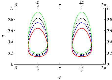
Figure S5: Analytical estimate of the regularization boundaries in the suppressory $\varphi-\eta$ control plane. Boundary function (cf. Eq. S31) encircling the region where chaos is suppressed in the $\varphi-\eta$ control plane for four values of the shape parameter: $m=0$ (dashed line), $m=0.717\simeq m_{\max}^{impulse}$ (solid line), $m=0.93$ (dotted line), and $m=0.96$ (thin solid line). System parameters as in Fig. S4.

I.3 Energy-based analysis

By analyzing the variation of the Duffing oscillator’s energy, one straightforwardly obtains an alternative physical explanation of the foregoing MA-based predictions. Indeed, Eq. 2 in the main text has the associated energy equation

$$\frac{dE}{dt}=-\delta\overset{.}{x}^{2}+\gamma\overset{.}{x}\sin\left(\omega t\right)-\beta\eta\overset{.}{x}x^{3}f(t),$$ (S35)

where, for the sake of convenience, we introduced the shift $t\rightarrow t+T/4$, and hence $\varphi\rightarrow\varphi-\pi/2$, and where $E(t)\equiv\left(1/2\right)\overset{.}{x}^{2}\left(t\right)+U\left[x\left(t\right)\right]$ $\left[U(x)\equiv-x^{2}/2+\beta x^{4}/4\right]$ is the energy function. Integration of Eq. S35 over any interval $\left[nT,nT+T/2\right]$, $n=0,1,2,...$, yields

$$E\left(nT+T/2\right) =E(nT)-\delta\int_{nT}^{nT+T/2}\overset{.}{x}^{2}\left(t\right)dt-\beta\eta\int_{nT}^{nT+T/2}\overset{.}{x}\left(t\right)x^{3}\left(t\right)f\left(t\right)dt$$

$$+\gamma\int_{nT}^{nT+T/2}\overset{.}{x}\left(t\right)\sin\left(\omega t\right)dt.$$ (S36)

Now, if we consider fixing the parameters $\left(\delta,\gamma,\beta,T\right)$ for the Duffing oscillator to undergo chaotic behaviour at $\eta=0$, there always exists an $n=n^{\ast}$ such that the energy increment $\Delta E\equiv$ $E\left(n^{\ast}T+T/2\right)-E(n^{\ast}T)$ is positive before chaotic escape from one of the two potential wells. Thus, after applying  the first mean value theorem for integrals S_5 together with well-known properties of the Jacobian elliptic functions S_1 to the last two integrals on the right-hand side of Eq. S36,

$$E\left(n^{\ast}T+T/2\right) =E(n^{\ast}T)-\delta\int_{n^{\ast}T}^{n^{\ast}T+T/2}\overset{.}{x}^{2}\left(t\right)dt+\frac{\gamma T}{\pi}\overset{.}{x}\left(t^{\ast}\right)$$

$$-\frac{\beta\eta T\overset{.}{x}\left(t^{\ast\ast}\right)x^{3}\left(t^{\ast\ast}\right)}{2}F\left(\varphi,m\right),$$ (S37)

where $t^{\ast},t^{\ast\ast}\in\left[n^{\ast}T,n^{\ast}T+T/2\right]$ and

$$F\left(\varphi,m\right)\equiv\frac{\sqrt{1-m}N(m)}{K(m)}\operatorname{sd}\left[\frac{2K(m)\varphi}{\pi}\right],$$ (S38)

with $\operatorname{sd}\left(\cdot\right)\equiv\operatorname{sn}\left(\cdot;m\right)/\operatorname*{dn}\left(\cdot;m\right)$ being the Jacobian elliptic function of parameter $m$, one has

$$\gamma T\overset{.}{x}\left(t^{\ast}\right)/\pi>\delta\int_{n^{\ast}T}^{n^{\ast}T+T/2}\overset{.}{x}^{2}\left(t\right)dt$$ (S39)

at $\eta=0$ when the Duffing oscillator exhibits chaotic behaviour. It is straightforward to see that $F\left(\varphi,m\right)$ presents an absolute maximum (minimum) at $m=m_{\max}^{impulse}\simeq 0.717,\varphi=\pi/2$ ($m=m_{\max}^{impulse}\simeq 0.717,\varphi=3\pi/2$). It is a $2\pi$-periodic function in $\varphi$, and presents the noteworthy properties (see Fig. S6):

$$F\left(\pi/2,m\right) =-F\left(3\pi/2,m\right)=\frac{N(m)}{K(m)}=2I(m),$$ (S40)

$$F\left(0,m\right) =F\left(\pi,m\right)=0,$$ (S41)

$$\lim_{m\rightarrow 1}F\left(\pi/2,m\right) =\lim_{m\rightarrow 1}F\left(3\pi/2,m\right)=0,$$ (S42)

$$\lim_{m\rightarrow 0}F\left(\pi/2,m\right) =-\lim_{m\rightarrow 0}F\left(3\pi/2,m\right)=\frac{2}{\pi}.$$ (S43)

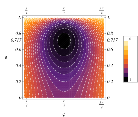
Figure S6: Function $F\left(\varphi,m\right)$ describing the effect of the SE’s impulse in the energy equation. Contour plot of the function $F\left(\varphi,m\right)$ (see Eq. S38) versus the initial phase difference $\varphi$ and the shape parameter $m$ showing an absolute maximum at $\varphi=\varphi_{opt}=\pi/2,m=m_{\max}^{impulse}\simeq 0.717$. Note that the region around the value $\varphi=\varphi_{opt}=3\pi/2$ is not shown because of the symmetry $F\left(\pi/2,m\right)=-F\left(3\pi/2,m\right)=N(m)/K(m)$ (cf. Eq. S40).

In this situation, one lets the elliptic SE act on the Duffing oscillator while holding the remaining parameters constant. For sufficiently small values of $\eta>0$, one expects that both the dissipation work (the integral in Eq. S37) and $\overset{.}{x}\left(t^{\ast}\right)$ will approximately maintain their initial values (at $\eta=0$) while the function $F\left(\varphi,m\right)$ will increase (decrease) from 0 (at $\varphi=0,\pi$), so that, in some cases depending upon the remaining parameters and the sign of $\overset{.}{x}\left(t^{\ast\ast}\right)x^{3}\left(t^{\ast\ast}\right)$, the energy increment just before the chaotic escape existing for $\eta=0$, $\Delta E$, could be sufficiently large and negative to suppress the initial chaotic state in the sense of leading the Duffing oscillator to the basin of a certain periodic attractor. Clearly, the probability of suppressing the initial chaotic state is maximal at $m=m_{\max}^{impulse}\simeq 0.717,\varphi=\pi/2\ \left(\varphi=3\pi/2\right)$ (i.e., when the impulse transmitted by the SE is maximum, cf. Eq. S40), which is in complete agreement with the foregoing MA-based predictions.

Remarkably, we can obtain an useful alternative estimate of the suppressory amplitude, $\eta^{\prime}$, by requiring that the sum of the two excitation terms in Eq. S37 be approximately cancelled:

$$\frac{\beta\eta^{\prime}\overset{.}{x}\left(t^{\ast\ast}\right)x^{3}\left(t^{\ast\ast}\right)}{2}F\left(\varphi,m\right)\approx\frac{\gamma}{\pi}\overset{.}{x}\left(t^{\ast}\right).$$ (S44)

In such a case, the remaining integral in Eq. S37 (dissipation work) yields an energy decrease over time which suppresses the initial chaotic state, ultimately leading the Duffing oscillator to small-amplitude periodic oscillations around some of the two fixed points $\left(x=\pm\beta^{-1/2},\overset{.}{x}=0\right)$ of the unperturbed Duffing oscillator $\left(\delta=\gamma=\eta=0\right)$. From the properties of the function $F\left(\varphi,m\right)$ (cf. Eqs. S40-S43), one sees that the lower values of $\eta^{\prime}$ are obtained for $\varphi=\varphi_{opt}=\left\{\pi/2,3\pi/2\right\}$, and hence an alternative estimate of the upper suppressory amplitude, $\eta_{\max}^{\prime}$, reads

$$\frac{\eta_{\max}^{\prime}(m)}{\eta_{\max}^{\prime}(m=0)}\approx\frac{2/\pi}{\left|F\left(\pm\pi/2,m\right)\right|}\equiv\frac{2K(m)}{\pi N(m)}\equiv\left[\frac{I(m)}{I(m=0)}\right]^{-1},$$ (S45)

which presents a single minimum at $m=m_{\max}^{impulse}\simeq 0.717$, while its behaviour, as a function of the shape parameter, is similar to that of the MA-based upper suppressory amplitude (cf. Eq. S23):

$$\frac{\eta_{\max}(m,T)}{\eta_{\max}(m=0,T)}=\left[\frac{a_{0}(m)}{a_{0}(m=0)}+\sum_{p=1}^{\infty}\frac{a_{p}(m)b_{p}(T)}{a_{0}(m=0)b_{0}(T)}\right]^{-1}.$$ (S46)

It is worth noticing that the approximate character of the suppressory condition given by Eq. S44 prevents us from ensuring that, even in certain cases corresponding to particular values of the initial conditions and system parameters, the SE can effectively lead the Duffing oscillator to some of the two fixed points $\left(x=\pm\beta^{-1/2},\overset{.}{x}=0\right)$. Indeed, Eq. S37 tell us that any decrease of the Duffing oscillator’s energy over half a period implies a subsequent decrease of the dissipation work over the next half a period, such that this decrease process continues until some of the mismatches of the (approximate) cancellation of the two excitation terms is sufficiently large to compensate the dissipation work in the sense of yielding an increase of the energy, over a certain half a period, and a subsequent energy oscillation later. This means that the steady behaviour becomes a small-amplitude periodic oscillation around some of the fixed points from a certain instant $t=n^{s}T$, while the corresponding dissipation work is proportional to the action of the periodic orbit in the phase space:

$$\delta\int_{n^{s}T}^{n^{s}T+T/2}\overset{.}{x}^{2}\left(t\right)dt=\delta\int_{n^{s}T}^{n^{s}T+T/2}\overset{.}{x}\left(t\right)dx=\delta\pi J,$$ (S47)

where $J\equiv\frac{1}{2\pi}\oint pdq$ is the action integral S_6 . Alternatively, one can show the same behavior as follows. After linearizing Eq. (2) in the main text around $x=\pm\beta^{-1/2}$, one straightforwardly obtains the equation governing the linear stability of the two equilibria:

$$\overset{..}{z}+\omega_{0}^{2}z=-\delta\overset{.}{z}-\eta\left(3z\pm\beta^{-1/2}\right)f(t)+\gamma\cos\left(\omega t\right),$$ (S48)

where $\omega_{0}\equiv\sqrt{2}$ and $z\equiv x\mp\beta^{-1/2}$, respectively. Equation S48 has the associated energy equation

$$\frac{dE_{0}}{dt}=-\delta\overset{.}{z}^{2}+\gamma\overset{.}{z}\sin\left(\omega t\right)-\eta\left(3z\pm\beta^{-1/2}\right)zf(t),$$ (S49)

where we introduced the shift $t\rightarrow t+T/4$, and hence $\varphi\rightarrow\varphi-\pi/2$, and where $E_{0}(t)\equiv\left(1/2\right)\overset{.}{z}^{2}\left(t\right)+U_{0}\left[z\left(t\right)\right]$ $\left[U_{0}(z)\equiv\omega_{0}^{2}z^{2}/2\right]$ is the energy function of the linearized system. Integration of Eq. S49 over any interval $\left[nT,nT+T/2\right]$, $n=0,1,2,...$, yields

$$E_{0}\left(nT+T/2\right) =E_{0}(nT)-\delta\int_{nT}^{nT+T/2}\overset{.}{z}^{2}\left(t\right)dt+\gamma\int_{nT}^{nT+T/2}\overset{.}{z}\left(t\right)\sin\left(\omega t\right)dt$$

$$-\eta\int_{nT}^{nT+T/2}\overset{.}{z}\left(t\right)\left[3z(t)\pm\beta^{-1/2}\right]f\left(t\right)dt.$$ (S50)

After applying  the first mean value theorem for integrals together with well-known properties of the Jacobian elliptic functions to the last two integrals on the right-hand side of Eq. S50, one obtains

$$E_{0}\left(nT+T/2\right) =E_{0}(nT)-\delta\int_{nT}^{nT+T/2}\overset{.}{z}^{2}\left(t\right)dt+\frac{\gamma T}{\pi}\overset{.}{z}\left(t^{\prime}\right)$$

$$-\frac{\eta T\overset{.}{z}\left(t^{\prime\prime}\right)\left[3z(t^{\prime\prime})\pm\beta^{-1/2}\right]}{2}F\left(\varphi,m\right),$$ (S51)

where $t^{\prime},t^{\prime\prime}\in\left[nT,nT+T/2\right]$. Note that the suppressory condition given by Eq. S44 implies the approximate cancellation of the sum of the two excitation terms in Eq. S51, and hence the same reasoning applied above to the general energy $E$ can now be directly applied to the small-amplitude energy $E_{0}$ (compare Eqs. S37 and S51), thus allowing us to conclude that the regularized small-amplitude periodic oscillations around any of the fixed points $\left(x=\pm\beta^{-1/2},\overset{.}{x}=0\right)$ are linearly stable attractors.

II Numerical methods

In our numerical simulations, we studied the purely deterministic case as well as the robustness of the impulse-induced chaos-control scenario against the presence of additive noise in the Duffing equation:

$$\overset{..}{x}=x-\beta\left[1+\eta f(t)\right]x^{3}-\delta\overset{.}{x}+\gamma\cos\left(\omega t\right)+\sqrt{\sigma}\xi\left(t\right),$$ (S52)

where $\xi\left(t\right)$ is a Gaussian white noise with zero mean and $\left\langle\xi\left(t\right)\xi\left(t+s\right)\right\rangle=\delta\left(s\right)$, and $\sigma=2k_{b}T^{\ast}$ with $k_{b}$ and $T^{\ast}$ being the Boltzmann constant and temperature, respectively. For the sake of completeness, we computed three types of complementary diagrams.

On the one hand, we compare the theoretical predictions obtained from MA with the Lyapunov exponent (LE) calculations for Eq. S52. In this regard, it is worth recalling that, even in the case of small values of $\gamma,\delta$ and $\eta$, one cannot expect too good a quantitative agreement between these two kinds of approaches because MA is a perturbative technique generally related to transient chaos, while LE provides information solely concerning steady responses. We computed the LEs using a version of the algorithm introduced in S_7 , with integration typically up to $10^{4}$ drive cycles for each fixed set of parameters. In the absence of the SE $\left(\eta=0\right)$, the Eq. S52 with $\sigma=0,\delta=0.25,\gamma=0.29,\beta=1,\omega=1$ exhibits a strange chaotic attractor with a maximal LE $\lambda^{+}\left(\eta=0\right)=0.025$ bits/s. To construct the LE diagrams we followed two steps. First, the maximal LE was calculated for each point on a $N\times N$ grid with phase difference $\varphi$ and amplitude $\eta$ along the horizontal and vertical axes. Second, a diagram was constructed by only plotting points on the grid according to a colour code.

On the other hand, we computed period-distribution and isospike diagrams S_8 to obtain detailed information regarding the periodicity order of the regularized solutions as well as useful information regarding the complexity of their waveforms in the $\varphi-\eta$ control plane. Isospike diagrams are based on computing the number of local maxima per period for the periodic solutions after a sufficiently long transient for each point on a $N\times N$ grid with phase difference $\varphi$ and amplitude $\eta$ along the horizontal and vertical axes. To this end, after the first $10^{4}$ drive cycles, we continued the integration for $200$ additional drive cycles recording up to $800$ extrema (maxima and minima) of the variable of interest and checking whether pulses repeated or not. In isospike diagrams, black is used to represent chaos; i.e., lack of numerically detected periodicity. To represent maxima, we used a palette of 17 colors. Patterns with more than 17 maxima are plotted by recycling the 17 basic colors modulo 17. Period-distribution diagrams are based on computing the period of periodic solutions after a sufficiently long transient ($10^{4}$ drive cycles) for each point on a $N\times N$ grid with phase difference $\varphi$ and amplitude $\eta$ along the horizontal and vertical axes. In period-distribution diagrams we used a colour code to detect periodic solutions with periods between $T$ (period-1 solution) and $8T$ (period-8 solution). In period-distribution diagrams, black is used to represent chaos; i.e., lack of numerically detected periodicity.

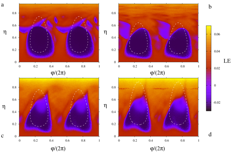
Figure S7: Robustness of the impulse-induced chaos-control scenario against the presence of noise. LE diagrams in the $\varphi-\eta$ control plane in the presence of noise for four values of the shape parameter: a, $m=0$; b, $m=0.717\simeq m_{\max}^{impulse}$; c, $m=0.9$; d, $m=0.95$. The white contours indicate the respective predicted boundary functions for the purely deterministic case (cf. Eq. S31) which are symmetric with respect to the optimal suppressory values of the initial phase difference. Noise strength: $\sigma=0.006$, and the remaining parameters as in Fig. S4.

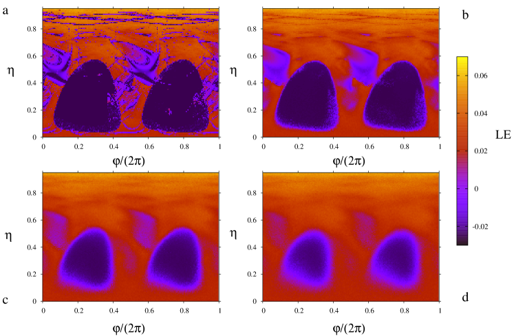
Figure S8: Robustness of the maximal islands of regularization against increasing noise. LE diagrams in the $\varphi-\eta$ control plane for four values of the noise strength: a, $\sigma=0$ (purely deterministic case); b, $\sigma=0.002$; c, $\sigma=0.018$; d, $\sigma=0.038$. Shape parameter: $m=0.717\simeq m_{\max}^{impulse}$, and the remaining parameters as in Fig. S4.

We studied the evolution of the regularization regions in the $\varphi-\eta$ control plane as the impulse transmitted by the SE is changed from its value at $m=0$ to its value at an $m$ value very close to $1$ by computing LE, isospike, and period-distribution diagrams. For the purely deterministic case, the results are respectively shown in Figs. 4, 5, and 6 of the main text, while Fig. S7 shows, for the same set of fixed parameters, four illustrative LE diagrams for the Duffing oscillator in the presence of noise $\left(\sigma>0\right)$. Although the presence of noise gives systematically rise to a decrease, or even a complete elimination, of secondary and minor islands of regularization in the $\varphi-\eta$ control plane (see Fig. S8), a comparison between the purely deterministic case $\left(\sigma=0\right)$ and the noisy case $\left(\sigma>0\right)$ for the same values of the shape parameter (compare Fig. 4 in the main text with Fig. S7) indicates that the impulse-induced chaos-control scenario is robust against the presence of moderate noise.

III Experimental methods

The experimental setup used in our analog implementation of the damped driven Duffing oscillator (Eq. 2 in the main text) is shown in Fig. S9. The circuit is governed by the equation

$$\zeta^{-2}\overset{..}{x} =x-\left[1+\eta f(t)\right]x^{3}-\zeta^{-1}\delta\overset{.}{x}+\gamma\cos\left(2\pi f_{d}t\right),$$ (S53)

$$f(t) \equiv a_{0}(m)\sin\left(2\pi f_{c}t+\varphi\right)+a_{1}(m)\sin\left(6\pi f_{c}t+3\varphi\right),$$ (S54)

where $\zeta=\left(RC\right)^{-1}$ with $R=10$ k$\Omega$, $C=10$ nF, while $\gamma=0.29$ and $f_{d}=1592.500$ Hz are the amplitude and frequency of the chaos-inducing signal, respectively, $\delta=0.25$, and $f(t)$ is the two-harmonics approximation of the elliptic SE (cf. Eq. S7). After the transformation $t\rightarrow\zeta^{-1}t$, Eq. S53 transforms into the dimensionless Eq. 2 in the main text with $\omega=1$. In the absence of any elliptic SE $\left(\eta=0\right)$, the circuit exhibits steady chaos for the above set of fixed parameters. The Duffing oscillator block with outputs $x$ and $y$ which is shown in Fig. S9 has been detailed described in Ref. S_9 .

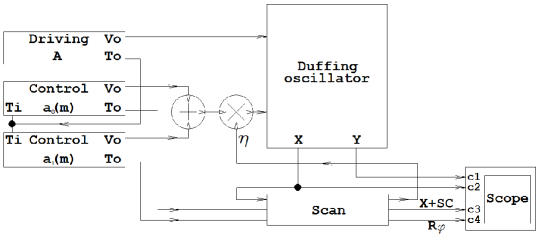
Figure S9: Scheme of the Duffing’s oscillator circuit. Blocks diagram of a damped two-well Duffing oscillator driven by a sinusoidal chaos-inducing signal and subjected to an elliptic suppressory signal in the form of a parametric perturbation of the cubic term. It includes the damped Duffing oscillator block with outputs $x$ and $y$, a driving block which generates the sinusoidal chaos-inducing signal, while the control blocks generate the two-harmonics approximation of the elliptic suppressory signal. The scan block performs an automatic scanning of the initial phase difference $\varphi$ and the suppressory amplitude $\eta$ through the ramp signal $R_{\phi}$ and the staircase signal $SC$.

The initial phase difference $\varphi$ has been implemented by selecting the frequency of the suppressory signal as $f_{c}=f_{d}+1/T_{sw}$ with $T_{sw}$ being the sweeping phase period during which a phase variation of $2\pi$ occurs, with $T_{sw}=2$ s in the experiments. The scan block generates two signals: a linear ramp $R_{\phi}$ for a phase variation of $2\pi$ and a $50$ levels staircase signal $SC$ (constant in amplitude during one phase sweep) allowing us to perform a sweeping of the suppressory amplitude $\eta$. The $x$ and $y$ signals from the Duffing oscillator block together with the phase-ramp and the $x+SC$ signals are monitored on a four trace oscilloscope.

Unlike the technique used in Ref. S_10 , where a real-time automatic indicator was considered to discriminate between regular (periodic) and chaotic behaviour, we inspect here the temporal series of the $x$ response signal for each point of the control-plane region $\varphi\in\left[0,2\pi\right],\eta\in\left[0,1\right]$ according to the aforementioned resolution. This procedure provides us not only a reliable discrimination between chaotic and periodic responses but also to discriminate whether the periodic responses are low-energy orbits around some of the two fixed points $\left(x=\pm\beta^{-1/2},\overset{.}{x}=0\right)$ of the unperturbed Duffing oscillator $\left(\delta=\gamma=\eta=0\right)$ or higher-energy orbits encircling both fixed points.

Acknowledgements

P.J.M. and R.C. acknowledge financial support from the Ministerio de Economía y Competitividad (MINECO, Spain) through FIS2011-25167 and FIS2012-34902 projects, respectively. R.C. acknowledges financial support from the Junta de Extremadura (JEx, Spain) through project GR15146. J. A. C. G. was supported by CNPq, Brazil.

References

(1)G. Chen and X. Dong, From Chaos to Order (World
Scientific, Singapore, 1998).
(2)R. Chacón, Control of Homoclinic Chaos by Weak
Periodic Perturbations (World Scientific, Singapore, 2005).
(3)Handbook of Chaos Control, 2nd ed., edited by E.
Schöll and H. G. Schuster (Wiley-VCH, Weinheim, 2008).
(4)G. Cicogna and L. Fronzoni, Phys. Rev. A 42, 1901 (1990).
(5)A. Azevedo and S. M. Rezende, Phys. Rev. Lett. 66, 1342 (1991).
(6)Y. Braiman and I. Goldhirsch, Phys. Rev. Lett. 66, 2545 (1991).
(7)E. R. Hunt, Phys. Rev. Lett. 68, 1953 (1991).
(8)R. Roy, T. W. Murphy, T. D. Maier, Z. Gills, and E. R. Hunt, Phys.
Rev. Lett. 68, 1259 (1992).
(9)S. Rajasekar, Pramana J. Phys. 41, 295 (1993).
(10)R. Meucci, W. Gadomski, M. Ciofini, and F. T. Arecchi, Phys. Rev.
E 49, R2528 (1994).
(11)S. J. Schiff, K. Jerger, D. H. Duong, T. Chang, M. L. Spano, and
W. L. Ditto, Nature (London) 370, 615 (1994).
(12)Z. Qu, G. Hu, G. Yang, and G. Qin, Phys. Rev. Lett. 74,
1736 (1995).
(13)V. N. Chizhevsky and R. Corbalán, Phys. Rev. E 54,
4576 (1996).
(14)J. Yang, Z. Qu, and G. Hu, Phys. Rev. E 53, 4402 (1996).
(15)D. Dangoisse, J.-C. Celet, and P. Glorieux, Phys. Rev. E56, 1396 (1997).
(16)A. Uchida, T. Sato, T. Ogawa, and F. Kannari, Phys. Rev. E
58, 7249 (1998).
(17)S. Alonso, F. Sagués, and A. S. Mikhailov, Science
299, 1722 (2003).
(18)H. Cao, X. Chi, and G. Chen, Int. J. Bifurcation Chaos Appl. Sci.
Eng. 14, 1115 (2004).
(19)S. Zambrano, J. M. Seoane, I. P. Mariño, M. A. F.
Sanjuán, S. Euzzor, R. Meucci, and F. T. Arecchi, New J. Phys.
10, 073030 (2008).
(20)R. Meucci, S. Euzzor, E. Pugliese, S. Zambrano, M. R. Gallas, and
J. A. C. Gallas, Phys. Rev. Lett. 116, 044101 (2016).
(21)S. H. Strogatz, Nonlinear Dynamics and Chaos
(Addison-Wesley, Reading, 1994).
(22)R. Chacón, M. Yu. Uleysky, and D. V. Makarov, Europhys. Lett.
90, 40003 (2010).
(23)M.-D. Wei and C.-C. Hsu, Opt. Commun. 285, 1366 (2012).
(24)P. J. Martínez and R. Chacón, Phys. Rev. Lett.
100, 144101 (2008).
(25)See Supplemental Material
(26)J. Guckenheimer and P. Holmes, Nonlinear Oscillations,
Dynamical Systems, and Bifurcations of Vector Fields (Springer-Verlag, New
York, 1983).
(27)F. C. Moon, Phys. Rev. Lett. 53, 962 (1984).
(28)R. Chacón, Phys. Rev. A 85, 013813 (2012).
(29)J. C. Gonzalez-Henao, E. Pugliese, S. Euzzor, S. F. Abdalah, R.
Meucci, and J. A. Roversi, Sci. Rep.5, 13152 (2015).

References

(1)Armitage, J. V & Eberlein, W. F. Elliptic Functions
(Cambridge University Press, 2006).
(2)Melnikov, V. K. On the stability of the center for time periodic
perturbations. Trans. Mosc. Math. Soc. 12, 1-57 (1963).
(3)Guckenheimer, J. & and Holmes, P. Nonlinear Oscillations,
Dynamical Systems, and Bifurcations of Vector Fields (Springer-Verlag, 1983).
(4)Chacón, R. Control of Homoclinic Chaos by Weak
Periodic Perturbations (World Scientific, 2005).
(5)Gradshteyn, I. S. & Ryzhik, I. M. Table of Integrals,
Series, and Products (Academic Press, 1980).
(6)Lichtenberg, A. J. & Lieberman, M. A. Regular and
Stochastic Motion (Springer-Verlag, 1983).
(7)Wolf, A., Swift, J. B., Swinney, H. L. & Vastano, J. A.
Determining Lyapunov exponents from a time series. Physica D 16,
285-317 (1985).
(8)Freire, J. G. & Gallas, J. A. C. Stern-Brocot trees in the
periodicity of mixed-mode oscillations. Phys. Chem. Chem. Phys.
13, 12191-12198 (2011).
(9)Meucci, R., Euzzor, S., Zambrano, S., Pugliese, E., Francini, F.
& Arecchi, F. T. Energy constraints in pulsed phase control of chaos.
Phys. Lett. A381, 82-86 (2017).
(10)Meucci, R., Euzzor, S., Pugliese, E., Zambrano, S., Gallas, M. R.
& Gallas, J. A. C. Optimal phase-control strategy for damped-driven Duffing
oscillators. Phys. Rev. Lett.116, 044101 (2016).