Fermionic bound states in Minkowski-space:
Light-cone singularities and structure

Abstract

The Bethe-Salpeter equation for two-body bound system with spin $1/2$ constituent is addressed directly in the Minkowski space. In order to accomplish this aim we use the Nakanishi integral representation of the Bethe-Salpeter amplitude and exploit the formal tool represented by the exact projection onto the null-plane. This formal step allows one i) to deal with end-point singularities one meets and ii) to find stable results, up to strongly relativistic regimes, that settles in strongly bound systems. We apply this technique to obtain the numerical dependence of the binding energies upon the coupling constants and the light-front amplitudes for a fermion-fermion $0^{+}$ state with interaction kernels, in ladder approximation, corresponding to scalar-, pseudoscalar- and vector-boson exchanges, respectively. After completing the numerical survey of the previous cases, we extend our approach to a quark-antiquark system in $0^{-}$ state, taking both constituent-fermion and exchanged-boson masses, from lattice calculations. Interestingly, the calculated light-front amplitudes for such a mock pion show peculiar signatures of the spin degrees of freedom.

1 Introduction

The standard approach to the relativistic bound state problem in quantum field theory was formulated, more than a half century ago, in a seminal work by Salpeter and Bethe BS51 . In principle, the Bethe-Salpeter equation (BSE) (see also the review Nakarev ) allows one to access the non perturbative regime of the dynamics inside a relativistic interacting system, as the Schrödinger equation does in a non relativistic regime. As it is well-known, apart the celebrated Wick-Cutkosky model wick1954properties ; cutkosky1954solutions , composed by two scalars exchanging a massless scalar, solving BSE is very difficult when one adopts the variables of the space where the physical processes take place, namely the Minkowski space. Furthermore the irreducible kernel itself cannot be written in a closed form. Nonetheless, in hadron physics, it could be highly desirable to develop non perturbative tools in Minkowski space suitable for supporting, e.g., experimental efforts that aim at unraveling the 3D structure of hadrons. It should be pointed out that the leading laboratories, like CERN (see Ref. adolph2013hadron , for recent COMPASS results) and JLAB (see, e.g., Ref. avakian2016studies ), as well as the future Electron-Ion Collider, have dedicated program focused on the investigations of Semi-inclusive DIS processes, i.e. the main source of information on the above issue.

Moreover, on the theory side we mention the present attempts of getting parton distributions as a limiting procedure applied to imaginary-time lattice calculations, following the suggestion of Ref. XJIPRL13 (see Ref.AlexPRD15 , for some recent lattice calculations), as well as the strong caveat contained in Ref. rossi2017note . All that motivates a detailed presentation of our novel method of solving BSE with spin degree of freedom in Minkowski space, which in perspective could give some reliable contribution to the coherent efforts toward an investigation of the 3D tomography of hadrons.

Our method is based on the so-called Nakanishi integral representation (NIR) of the Bethe-Salpeter (BS) amplitude (see, e.g., Ref. FSV1 for a recent introduction to the issue, and references quoted therein). This representation is given by a suitable integral of the Nakanishi weight-function (a real function) divided by a denominator depending upon both the external four-momenta and the integration variables. In this way, one has an explicit expression of the analytic structure of the BS amplitude, and proceeds to formal elaborations. We anticipate that the validity of NIR for obtaining actual solutions of the ladder BSE, i.e. the one we have investigated, is achieved a posteriori, once an equivalent generalized eigenvalue problem is shown to admit solutions. Within the NIR approach that will be illustrated in detail for the two-fermion case in what follows, several studies have been carried out. Among them, one has to mention the works devoted to the investigation of: (i) two-scalar bound and zero-energy states, in ladder approximation with a massive exchange Kusaka ; CK2006 ; FSV2 ; Tomio2016 ; FSV3 , as well as two-fermion ground states CK2010 ; dFSV1 ; (ii) two scalars interacting via a cross-ladder kernel CK2006b ; gigante2017bound . A major difference, that separates the above mentioned studies in two groups, is the technique to deal with the BSE analytic structure in momentum space. In Refs. FSV2 ; Tomio2016 ; FSV3 ; dFSV1 ; gigante2017bound , it has been exploited the light-front (LF) projection, which amounts to eliminate the relative LF time, between the two particles, by integrating over the component $k^{-}=k^{0}-k^{3}$ of the constituent relative momentum (see Refs. Sales:1999ec ; SalPRC01 ; marinho2008light ; Frederico:2010zh ; FSV2 for details). Such an elegant and physically motivated procedure, based on the non-explicitly covariant LF quantum-field theory (see Ref.Brod_rev ), perfectly combines with NIR, and, as discussed in the next Sections, it allows one to successfully deal with singularities (see Ref. Yan for an early discussion of those singularities) that stem from the spin degrees of freedom acting in the problem. In general, the LF projection is able to exactly transform BSE in Minkowski space into a numerically affordable integral equation for the Nakanishi weight function, without resorting to the so-called Wick rotation wick1954properties . Specifically, the ladder BSE is transformed into a generalized eigenvalue-problem, where the Nakanishi-weight functions play the role of eigenvectors. Differently, Refs. CK2006 ; CK2006b ; CK2010 adopted a formal elaboration based on the covariant version of the LF quantum-field theory CK_rev . This approach has not allowed to formally identify the singularities that plague BSE with spin degrees of freedom, and therefore, in this case, the eigenvalue equations to be solved are different from the ones we get. In particular, in Ref. CK2010 the $0^{+}$ two-fermion case is studied and a smoothing function is introduced for achieving stable eigenvalues (indeed the eigenvalues are the coupling constants, as shown in what follows). It should be pointed out that in the range of the binding energies explored in Ref. CK2010 , $B/m\in[0.01-0.5]$ ($m$ is the mass of the constituents), the eigenvalues fully agree with the outcomes of our elaboration for all the three interaction kernels considered (see dFSV1 and the next Sections). As to the eigenvectors, the only case discussed in CK2010 is in an overall agreement with our results (cf Sect. 6).

Aim of this work is to extend our previous investigations of the ladder BSE FSV1 ; FSV2 ; Tomio2016 ; FSV3 ; dFSV1 ; Pimentel:2016cpj for a $0^{+}$ two-fermion system, interacting through the exchange of massive scalar, pseudoscalar or vector bosons. Since Ref. dFSV1 was basically devoted to validate our method through the comparison of the obtained eigenvalues and the ones found in the literature, in the present paper we first provide the non trivial details of the formal approach, that can be adopted for future studies of systems with higher spins. Then we illustrate: i) for each interaction above mentioned, physical motivations for the numerical dependence of the binding energy upon the coupling constant $g^{2}$ we have got; and ii) the peculiar outcomes of the NIR+LF framework, represented by the eigenvectors of our coupled integral system. Let us recall that the eigenvectors are the Nakanishi-weight functions, namely the fundamental ingredient for recovering both the full BS amplitude and the LF amplitudes. Furthermore, we extend our analysis to a fermion-antifermion pseudoscalar system with a large binding energy, i.e. in a strongly relativistic regime. In particular, after tuning both the fermion mass and the mass of the exchanged vector-boson to the values suggested by lattice calculations, we show the LF amplitudes for such a mock pion. They feature the effects due to the spin degrees of freedom, and show the peculiarity of an approach addressing BSE directly in Minkowski space. This preliminary study, once it will be enriched with suitable phenomenological features, could be relevant in providing the initial scale for evolving pion transverse-momentum distributions (TMD) BaccJHEP15 .

The present paper is organized as follows. In section 2, we introduce 1) the basic equation for the homogeneous two-fermion Bethe-Salpeter equation, with a kernel in ladder approximation, based on three different kinds of massive exchanges, i.e. scalar, pseudoscalar and vector bosons; and 2) the general notation for the BS amplitude of a two-fermion $0^{+}$ state. In section 3, we illustrate the Nakanishi integral representation for the $0^{+}$ bound state of two fermions and review the LF projection technique, that allows one to formally infer an integral equation fulfilled by the Nakanishi weight function. In section 4, we introduce our distinctive method for formally obtaining the kernel of the integral equation fulfilled by the Nakanishi weight-function, and separate out the light-cone non-singular and singular contributions, by carefully analyzing the end-point singularities, related to the spin degree of freedom of the problem we are coping with. In section 5, we provide our numerical tools for solving the integral equation for the Nakanishi weight function, that is formally equivalent to get solution of the BSE in Minkowski space. In section 6, we discuss several numerical results for a two-fermion $0^{+}$ state, ranging from the dependence of the binding energy upon the coupling constant, peculiar for the three exchanges we consider to compute the LF amplitudes, building blocks of both LF distributions and TMDs. In a forthcoming paper dFSV2 we aim to address phenomenological, but realistic 4D kernel to study TMDs BarPRep02 . In section 7, we present an initial investigation of a fermion-antifermion $0^{-}$ state, featuring a mock pion, with input parameters inspired by standard lattice calculations. In section 8, we provide a summary and concluding remarks to close our work.

2 General formalism for the two-fermion homogeneous BSE

In this Section, the general formalism adopted for obtaining actual solutions of the BSE for a bound system composed by two spin-$1/2$ constituents is presented. Though the approach based on NIR is quite general, and it can be extended at least to BSE with analytic kernels, given our present knowledge, the ladder approximation is suitable to start our novel investigation on fermionic BSE, since it allows us to cope with some fundamental subtleties without considering additional, but irrelevant for our most urgent aim, complications. We can anticipate that the mentioned issues are related to the singularities onto the light-cone Yan , and the efforts for elucidating them are an unavoidable formal step in order to extend the NIR approach to higher spins (e.g. vector constituents). Among the two-fermion bound systems, the simplest one to be addressed is given by a $0^{+}$ bound state, that after taking into account the intrinsic parity can be trivially converted into a $0^{-}$ fermion-antifermion composite state, once the charge conjugation is applied.

In what follows, we adopt i) the ladder approximation for the interaction kernels, modeling scalar, pseudoscalar or vector exchanges, and ii) no self-energy and vertex corrections, apart a scalar form factor to be attached at the interaction vertexes (see below). With those assumptions, the fermion-antifermion BS amplitude, $\Phi(k,p)$ fulfills the following integral equation CK2010

$$\Phi(k,p)=~{}S(k+p/2)~{}\int\frac{d^{4}k^{\prime}}{(2\pi)^{4}}~{}F^{2}(k-k^{\prime})~{}$$

$$\times i{\cal K}(k,k^{\prime})~{}\Gamma_{1}~{}\Phi(k^{\prime},p)~{}\widehat{\Gamma}_{2}~{}S(k-p/2)\,,$$ (1)

where the off-mass-shell constituents have four-momenta given by $p_{1(2)}=p/2\pm k$, with $p^{2}_{1(2)}\neq m^{2}$, $p=p_{1}+p_{2}$ is the total momentum, with $M^{2}=p^{2}$ the bound-state square mass, and $k=(p_{1}-p_{2})/2$ the relative four-momentum. The Dirac propagator is given by

$$S(k)=~{}i~{}{/\!\!\!k+m\over k^{2}-m^{2}+i\epsilon}~{}~{},$$ (2)

and $\Gamma_{i}$ are the Dirac structures of the interaction vertex we will consider in what follows, namely $\Gamma_{i}\equiv I,~{}\gamma_{5},~{}\gamma^{\mu}$, for scalar, pseudoscalar and vector interactions, respectively. Moreover, using the charge-conjugation $4\times 4$ matrix $C=i\gamma^{2}\gamma^{0}$, we define $\widehat{\Gamma}_{2}=C\,\Gamma_{2}^{T}\,C$, and

$$F(k-k^{\prime})={\mu^{2}-\Lambda^{2}\over(k-k^{\prime})^{2}-\Lambda^{2}+i\epsilon}$$ (3)

is a suitable interaction-vertex form factor. Besides the Dirac structure, the interaction vertex contains also a momentum dependence (due to the exchanged-boson propagation) as well as a coupling constant. In particular, depending on the interaction, one has the following expression for $i{\cal K}$ in Eq. (1)

• for the scalar case

  $$i{\cal K}^{(Ld)}_{S}(k,k^{\prime})=-ig^{2}~{}{1\over(k-k^{\prime})^{2}-\mu^{2}+i\epsilon},$$ (4)

• for the pseudoscalar one,

  $$i{\cal K}^{(Ld)}_{PS}(k,k^{\prime})=ig^{2}~{}{1\over(k-k^{\prime})^{2}-\mu^{2}+i\epsilon},$$ (5)

• and finally for a vector exchange, in the Feynman gauge,

  $$i{\cal K}^{(Ld)\mu\nu}_{V}(k,k^{\prime})=-ig^{2}~{}{g^{\mu\nu}\over(k-k^{\prime})^{2}-\mu^{2}+i\epsilon}.$$ (6)

The BS amplitude $\Phi(k,p)$ can be decomposed as follows CK2010

$$\Phi(k,p)=\sum_{i=1}^{4}S_{i}(k,p)~{}\phi_{i}(k,p)~{},$$ (7)

where $\phi_{i}$ are suitable scalar functions of $(k^{2},\,p^{2},\,k\cdot p)$ with well-defined properties under the exchange $k\to-k$, namely they have to be even for $i=1,2,4$ and odd for $i=3$. The allowed Dirac structures are given by the $4\times 4$ matrices $S_{i}$, viz

$$S_{1}(k,p)=\gamma_{5}\,,\,S_{2}(k,p)={/\!\!\!p\over M}\,\gamma_{5}\,,\,$$

$$S_{3}(k,p)={k\cdot p\over M^{3}}/\!\!\!p~{}\gamma_{5}-{1\over M}/\!\!\!k\gamma_{5}~{},$$

$$S_{4}(k,p)={i\over M^{2}}\sigma^{\mu\nu}p_{\mu}k_{\nu}~{}\gamma_{5}~{}.$$ (8)

They satisfy the following orthogonality relation

$$Tr\Bigl{[}S_{i}(k,p)~{}S_{j}(k,p)\Bigr{]}={\cal N}_{i}(k,p)~{}\delta_{ij}.$$ (9)

Multiplying both sides of Eq. (1) by $S_{i}$ and carrying out the traces, one reduces to a system of four coupled integral equations, written as

$$\phi_{i}(k,p)=ig^{2}(\mu^{2}-\Lambda^{2})^{2}\sum_{j}~{}\int{d^{4}k^{\prime\prime}\over(2\pi)^{4}}$$

$$\times{c_{ij}(k,k^{\prime\prime},p)\over\Bigl{[}({p\over 2}+k)^{2}-m^{2}+i\epsilon\Bigr{]}\,\Bigl{[}({p\over 2}-k)^{2}-m^{2}+i\epsilon\Bigr{]}}$$

$$\times{\phi_{j}(k^{\prime\prime},p)\over\Bigl{[}(k-k^{\prime\prime})^{2}-\mu^{2}+i\epsilon\Bigr{]}\,\Bigl{[}(k-k^{\prime\prime})^{2}-\Lambda^{2}+i\epsilon\Bigr{]}^{2}}~{},$$

(10)

with $i,j=1,~{}2,~{}3,~{}4$. The coefficients $c_{ij}$ are obtained by performing the convenient traces:

$$c_{ij}(k,k^{\prime\prime},p)={1\over{\cal N}_{i}(k,p)}~{}Tr\left\{S_{i}(k,p)\left({/\!\!\!p\over 2}+/\!\!\!k+m\right)\right.$$

$$\times~{}\Gamma_{1}\left.~{}S_{j}(k^{\prime\prime},p)\widehat{\Gamma}_{2}\left({/\!\!\!p\over 2}-/\!\!\!k-m\right)\right\}$$ (11)

and are explicitly given in A (see also Ref. CK2010 ). Notice that the coefficients for a pseudoscalar exchange and a vector can be easily obtained from the coefficients for a scalar interaction, as explained in A.

3 Nakanishi integral representation and the light-front projection

In the sixties, for a bosonic case, Nakanishi (see Ref. nak71 for all the details) proposed and elaborated a new integral representation for perturbative transition amplitudes, relying on the parametric expression of the Feynman diagrams. The key point in his formal approach is the possibility to express a $n$-leg transition amplitude as a proper folding of a weight function and a denominator that contains all the independent scalar products of the $n$ external four-momenta. Noteworthy, by using NIR, the analytic properties of the transition amplitudes are dictated by the above mentioned denominator. As a final remark, one should remind that the weight function is unique, as demonstrated by Nakanishi exploiting the analyticity of the transition amplitude, expressed through NIR (see nak71 ).

A step forward of topical interest was carried out in Ref. CK2010 , where the generalization to the fermionic ground state was presented. It should be reminded that originally NIR was established only for the bosonic case, with some caveat about a straightforward application to the fermions, as recognized by Nakanishi himself, that was aware of the possible tricky role of the numerator in the Dirac propagator.

Following the spirit of Ref. CK2010 , one can apply NIR to each scalar function in Eq. (7), tentatively generalizing the Nakanishi approach to the fermionic case. Let us recall that the denominator of a generic Feynman diagram contributing to the fermionic transition amplitudes has the same expression as in the boson case analyzed by Nakanishi Nakarev , and this is the main feature leading to NIR. In conclusion, one can write for each $\phi_{i}(k,p)$ in Eq. (7)

$$\phi_{i}(k,p)=\int_{-1}^{1}dz^{\prime}\int_{0}^{\infty}d\gamma^{\prime}{g_{i}(\gamma^{\prime},z^{\prime};\kappa^{2})\over\left[{k}^{2}+z^{\prime}p\cdot k-\gamma^{\prime}-\kappa^{2}+i\epsilon\right]^{3}},$$

(12)

where $\kappa^{2}=m^{2}-M^{2}/4$. For each scalar function of the BS amplitude it is associated one weight function or Nakanishi amplitude $g_{i}(\gamma^{\prime},z^{\prime};\kappa^{2})$, which is conjectured to be unique and encodes all the non perturbative dynamical information. The power of the denominator in Eq. (12) can be chosen as any convenient integer. Actually, the power 3 is adopted following Ref. CK2010 . The scalar functions $\phi_{i}(k,p)$ must have well-defined properties under the exchange $k\to-k$: even for $i=1,2,4$ and odd for $i=3$. Those properties can be straightforwardly translated to the corresponding properties of the Nakanishi weight-function $g_{i}(\gamma^{\prime},z^{\prime};\kappa^{2})$ under the exchange $z^{\prime}\to-z^{\prime}$, i.e. they must be even for $i=1,2,4$ and odd for $i=3$.

By inserting Eq. (12) in Eq. (10), one can write the fermionic BSE as a system of coupled integral equations, given by

$$\int_{-1}^{1}dz^{\prime}\int_{0}^{\infty}d\gamma^{\prime}{g_{i}(\gamma^{\prime},z^{\prime};\kappa^{2})\over\left[{k}^{2}+z^{\prime}p\cdot k-\gamma^{\prime}-\kappa^{2}+i\epsilon\right]^{3}}=$$

$$=g^{2}~{}\sum_{j}\int_{-1}^{1}dz^{\prime}\int_{0}^{\infty}d\gamma^{\prime}~{}{K}_{ij}(k,p;\gamma^{\prime},z^{\prime})~{}g_{j}(\gamma^{\prime},z^{\prime};\kappa^{2}),$$

(13)

where the kernel that includes also the Nakanishi denominator of the BS amplitudes on the rhs is

$${K}_{ij}(k,p;\gamma^{\prime},z^{\prime})=i(\mu^{2}-\Lambda^{2})^{2}$$

$$\times\int{d^{4}k^{\prime\prime}\over(2\pi)^{4}}~{}{c_{ij}(k,k^{\prime\prime},p)\over\Bigl{[}({p\over 2}+k)^{2}-m^{2}+i\epsilon\Bigr{]}~{}\Bigl{[}({p\over 2}-k)^{2}-m^{2}+i\epsilon\Bigr{]}}$$

$$~{}\times{1\over\Bigl{[}(k-k^{\prime\prime})^{2}-\Lambda^{2}+i\epsilon\Bigr{]}^{2}~{}\Bigl{[}(k-k^{\prime\prime})^{2}-\mu^{2}+i\epsilon\Bigr{]}}$$

$$\times{1\over\Bigl{[}{k^{\prime\prime}}^{2}+z^{\prime}p\cdot k^{\prime\prime}-\gamma^{\prime}-\kappa^{2}+i\epsilon\Bigr{]}^{3}}~{}.$$ (14)

It is necessary to stress that the validity of the NIR for the BS amplitude is verified a posteriori. Namely, if the generalized eigen-equation in Eq. (13) admits eigen-solutions then NIR can be certainly applied to the scalar function $\phi_{i}(k,p)$. Let us recall that Eq. (10) formally follows from the BSE in Eq. (1).

One can perform the four-dimensional integration on $k^{\prime\prime}$ in Eq. (3), obtaining

$${K}_{ij}(k,p;\gamma^{\prime},z^{\prime})=$$

$$={1\over 8\pi^{2}M^{2}}~{}~{}(\mu^{2}-\Lambda^{2})^{2}~{}\sum_{n=1}^{3}{\cal P}^{(n)}_{ij}(k,p;\gamma^{\prime},z^{\prime})~{},$$

(15)

where

$${\cal P}^{(1)}_{ij}(k,p;\gamma^{\prime},z^{\prime})=$$

$$={a^{0}_{ij}+a^{1}_{ij}~{}(p\cdot k)+a^{2}_{ij}~{}(p\cdot k)^{2}+a^{3}_{ij}~{}k^{2}\over[(1-z)~{}(k^{-}-k^{-}_{d})+i\epsilon]~{}[(1+z)~{}(k^{-}-k^{-}_{u})-i\epsilon]}$$

$$\times~{}\int^{1}_{0}dv~{}v^{2}~{}(1-v)^{2}~{}F(k^{-},\gamma,z;\gamma^{\prime},z^{\prime};v)$$ (16)

$${\cal P}^{(2)}_{ij}(k,p;\gamma^{\prime},z^{\prime})=$$

$$={b^{0}_{ij}+b^{1}_{ij}~{}(p\cdot k)+b^{2}_{ij}~{}(p\cdot k)^{2}+b^{3}_{ij}~{}k^{2}\over~{}[(1-z)~{}(k^{-}-k^{-}_{d})+i\epsilon]~{}[(1+z)~{}(k^{-}-k^{-}_{u})-i\epsilon]}$$

$$\times~{}\int^{1}_{0}dv~{}v^{2}~{}(1-v)^{3}~{}F(k^{-},\gamma,z;\gamma^{\prime},z^{\prime};v)$$ (17)

$${\cal P}^{(3)}_{ij}(k,p;\gamma^{\prime},z^{\prime})=$$

$$={d^{0}_{ij}+d^{1}_{ij}~{}(p\cdot k)\over[(1-z)~{}(k^{-}-k^{-}_{d})+i\epsilon]~{}[(1+z)~{}(k^{-}-k^{-}_{u})-i\epsilon]}$$

$$\times\int^{1}_{0}dv~{}v^{2}~{}(1-v)^{3}\Bigl{[}(p\cdot k)^{2}-M^{2}k^{2}\Bigr{]}$$

$$\times~{}F(k^{-},\gamma,z;\gamma^{\prime},z^{\prime};v)~{}~{},$$ (18)

and the coefficients $a^{k}_{ij}$, $b^{k}_{ij}$ and $d^{k}_{ij}$ are given in A. In the above equations, one has

$$k^{-}_{d}=-{M\over 2}+{2\over M(1-z)}(\gamma+m^{2})$$

$$k^{-}_{u}={M\over 2}-{2\over M(1+z)}(\gamma+m^{2})$$ (19)

where the the LF variables $k^{\pm}=k^{0}\pm k^{3}$ have been used, and the following notation has been adopted: $\gamma=|{\bf k}_{\perp}|^{2}$ and $z=-2k^{+}/M$ $\in[-1,1]$ (see Ref. FSV1 for details on this range). Moreover, in Eqs. (16), (17) and (18), one has

$$F(k^{-},\gamma,z;\gamma^{\prime},z^{\prime};v)={1\over\Bigl{[}k^{-}~{}k^{+}_{D}+\ell_{D}+i\epsilon\Bigr{]}^{2}}$$

$${3(k^{-}~{}k^{+}_{D}+\ell_{D})+(1-v)\Bigl{(}\mu^{2}-\Lambda^{2}\Bigr{)}\over\Bigl{[}k^{-}~{}k^{+}_{D}+\ell_{D}+(1-v)\Bigl{(}\mu^{2}-\Lambda^{2}\Bigr{)}+i\epsilon\Bigr{]}^{3}}$$ (20)

with

$$k^{+}_{D}=v(1-v){M\over 2}~{}(z^{\prime}-z)$$

$$\ell_{D}=-v(1-v)\Bigl{(}\gamma+zz^{\prime}{M^{2}\over 4}-{z^{\prime}}^{2}{M^{2}\over 4}\Bigr{)}$$

$$-v\Bigl{[}\gamma^{\prime}+z^{\prime 2}m^{2}+(1-z^{\prime 2})\kappa^{2}\Bigr{]}-(1-v)\mu^{2}~{}~{}.$$ (21)

By a direct inspection of Eq. (20), one can realize that several poles affect the needed integration on the relative four-momentum. In order to treat the poles in a proper way, we adopt the so-called LF-projection onto the null-plane (see, e.g.Sales:1999ec ; Frederico:2010zh ; marinho2008light ), that amounts to integrate over the LF component $k^{-}$ both sides of Eq. (13). It should be pointed out that such a LF-projection is specific of the non-explicitly covariant version of the LF framework, and it is a key ingredient in our approach, as it will be clear in the next Sections. As to the present stage of the elaboration, the LF projection marks one of the differences with the explicitly covariant approach in Ref. CK2010 .

To conclude this Section, it should be emphasized that the announced difficulties in the fermionic case are related to the possible light-cone singularities generated by powers of $k^{-}$ contained in the coefficients $c_{ij}(k,k^{\prime\prime},p)$ (see also Ref. Yan and Refs. Bakker:2007ota ; bakker2005restoring ; Melikhov:2002mp for more details on the light-cone singularities). In the next Sections, the singularities will be identified and formally integrated out.

3.1 Light-front projection of the fermionic Bethe-Salpeter equation

The integration of the lhs is straightforward, since it is analogous to the scalar case. After the LF projection one gets what we shortly call light-front amplitudes

$$\psi_{i}(\gamma,\xi)=\int{dk^{-}\over 2\pi}~{}\phi_{i}(k,p)=$$

$$=-{i\over M}\int_{0}^{\infty}d\gamma^{\prime}{g_{i}(\gamma^{\prime},z;\kappa^{2})\over\left[\gamma+\gamma^{\prime}+m^{2}z^{2}+(1-z^{2})\kappa^{2}-i\epsilon\right]^{2}}$$

where $\xi=(1-z)/2$ belongs to $[0,1]$. Notice that $\psi_{i}$ are scalar functions rotationally invariant into the transverse plane and they will be used for constructing dFSV2 the so-called valence component of the two-fermion state, once a Fock expansion of this state is introduced. In Eq. (3.1), $i\epsilon$ can be removed, since we are dealing with a bound state and $\kappa^{2}>0$.

Differently, the integration on $k^{-}$ of the rhs of Eq. (13) has to be done very carefully and it represents the core of our approach. A first, but short, presentation can be found in Ref. dFSV1 , together with some important numerical outcomes.

Then, performing the LF projection as in Eq. (3.1), one can transform Eq. (13) into a new coupled integral-equation system for the Nakanishi weight-functions, viz

$$\int_{0}^{\infty}d\gamma^{\prime}{g_{i}(\gamma^{\prime},z;\kappa^{2})\over\left[\gamma+\gamma^{\prime}+m^{2}z^{2}+(1-z^{2})\kappa^{2}\right]^{2}}=iMg^{2}$$

$$\times~{}\sum_{j}\int_{0}^{\infty}d\gamma^{\prime}\int_{-1}^{1}dz^{\prime}{\cal L}_{ij}(\gamma,z;\gamma^{\prime},z^{\prime})~{}g_{j}(\gamma^{\prime},z^{\prime};\kappa^{2})\,,$$

where

$${\cal L}_{ij}(\gamma,z;\gamma^{\prime},z^{\prime})=$$

$$={(\mu^{2}-\Lambda^{2})^{2}\over 8\pi^{2}M^{2}}~{}\int{dk^{-}\over 2\pi}\sum_{n=1}^{3}{\cal P}^{(n)}_{ij}(k,p;\gamma^{\prime},z^{\prime})~{},$$ (24)

This coupled system has the attractive feature that one has to deal with a single non compact variable, $\gamma^{\prime}$, and a compact one, $z^{\prime}$ (like for $\gamma$ and $z$, respectively).

In the next subsection the integration on $k^{-}$ in Eq. (24) will be discussed in detail.

3.2 The kernel operator of the coupled integral-equation system

One can write the kernel ${\cal L}_{ij}$ as follows

$${\mathcal{L}}_{ij}(\gamma,z;\gamma^{\prime},z^{\prime})={(\mu^{2}-\Lambda^{2})^{2}\over 8\pi^{2}M^{2}}\int^{1}_{0}dv~{}v^{2}~{}(1-v)^{2}\,$$

$$\times\sum_{n=0}^{3}F_{n;ij}(v,\gamma,z,p)~{}{\cal C}_{n}$$ (25)

where the non vanishing $F_{0;ij}$, $F_{1;ij}$, $F_{2;ij}$ and $F_{3;ij}$ are listed in Table 1.

Table 1: Non vanishing coefficients $F_{0;ij}$, $F_{1;ij}$, $F_{2;ij}$ and $F_{3;ij}$.

$~{}ij~{}$	$F_{0;ij}$	$F_{1;ij}$	$F_{2;ij}$	$F_{3;ij}$
$11$	$m^{2}+M^{2}/4+\gamma$	$zM/2$	$0$	$0$
$12$	$mM$	$0$	$0$	$0$
$14$	$-(1-v)\left(\gamma+z^{2}{M^{2}\over 16}\right)$	$-(1-v)zM/4$	$-(1-v)/4$	$0$
$21$	$mM$	$0$	$0$	$0$
$22$	$m^{2}+M^{2}/4-\gamma-z^{2}{M^{2}/8}$	$0$	$-(1/2)$	$0$
$23$	$(1-v)z\left(\gamma+z^{2}{M^{2}\over 16}\right)/2$	$-(1-v)\left(\gamma-z^{2}{M^{2}\over 16}\right)/M$	$-(1-v)z/8$	$-(1-v)/(4M)$
$24$	$-(1-v)\left(\gamma+z^{2}{M^{2}\over 16}\right)2m/(M)$	$-(1-v)zm/2$	$-(1-v)m/(2M)$	$0$
$32$	$-z{M^{2}/2}$	$M$	$0$	$0$
$33$	$(1-v)\Bigl{[}m^{2}-M^{2}/4+\gamma+z^{2}{M^{2}/8}\Bigr{]}$	$0$	$(1-v)/2$	$0$
$34$	$-(1-v)zmM/2$	$(1-v)m$	$0$	$0$
$41$	$M^{2}$	$0$	$0$	$0$
$42$	$2mM$	$0$	$0$	$0$
$43$	$-(1-v)zmM/2$	$(1-v)m$	$0$	$0$
$44$	$(1-v)\Bigl{[}m^{2}-M^{2}/4-\gamma\Bigr{]}$	$-(1-v)zM/2$	$0$	$0$

Moreover, in Eq. (25) the functions ${\cal C}_{n}$ are integrals over $k^{-}$ defined by

$${\cal C}_{n}=\int{dk^{-}\over 2\pi}{(k^{-})^{n}~{}F(k^{-},\gamma,z;\gamma^{\prime},z^{\prime};v)\over\Bigl{[}(1-z)k^{-}-(1-z)k^{-}_{d}+i\epsilon\Bigr{]}}$$

$$\times~{}{1\over\Bigl{[}(1+z)k^{-}-(1+z)k^{-}_{u}-i\epsilon\Bigr{]}}=$$

$$=-{\partial\over\partial\ell_{D}}\int{dk^{-}\over 2\pi}{(k^{-})^{n}\over\Bigl{[}(1-z)k^{-}-(1-z)k^{-}_{d}+i\epsilon\Bigr{]}}$$

$$\times~{}{1\over\Bigl{[}(1+z)k^{-}-(1+z)k^{-}_{u}-i\epsilon\Bigr{]}}$$

$$\times~{}{1\over\Bigl{[}k^{+}_{D}k^{-}+\ell_{D}+(1-v)\Bigl{(}\mu^{2}-\Lambda^{2}\Bigr{)}+i\epsilon\Bigr{]}^{2}}$$

$$\times~{}{1\over\Bigl{[}k^{+}_{D}k^{-}+\ell_{D}+i\epsilon\Bigr{]}}~{},$$ (26)

with $n=0,1,2,3$.

It is fundamental to notice that the powers of $k^{-}$ in the numerator of Eq. (26) are dictated by the coefficients $c_{ij}(k,k^{\prime\prime},p)$ (see Eq. (11)), that in turn are determined by the Dirac structures of both the BS amplitude (cf Eq. (7)) and the interaction vertexes (cf, e.g., the matrix $\Gamma_{i}$ in the ladder BSE in Eq. (1)). Since the power of $k^{-}$ in the numerator lead to singular integrals, as discussed below, one has to bring in mind that the most severe singularities can be determined in advance, once the Dirac structures above mentioned are known. Therefore, if one has to deal with the BS amplitude of a fermion-boson system or a vector-vector one, the biggest power of $k^{-}$ can be easily singled out after modeling (in agreement to the required symmetries and the interaction) the needed Dirac structures.

As it is clearly shown in Eq. (26), the $k^{-}$ integration of the kernel ${\cal L}_{ij}$ could become tricky if the powers of $k^{-}$ in the numerator are not suitably balanced by the ones in the denominator for some values of $k^{+}_{D}$. The values $z=\pm 1$, that in principle could generate troubles, are made harmless by the vanishing values of the Nakanishi weight functions at those values (see the discussion of the boundaries for the scattering case in Ref. FSV3 , that can be adapted to the present discussion). In conclusion, to perform the projection of the kernel ${K}_{ij}$ onto the LF hyper-plane, one has to carefully study the integrals ${\cal C}_{n}$. In particular, we should analyze the behavior of the integrand when the contour arc goes to infinity in order to use the Cauchy’s residue theorem in Eq. (26). The critical situation occurs for $k^{+}_{D}=0$, that was not recognized as the source of the instabilities met in Ref. CK2010 (they were fixed only through a numerical procedure). Indeed, to single out the actual sources of instabilities makes more sound the NIR approach for systems with spin degrees of freedom.

4 The integration on $k^{-}$ of the kernel ${\cal L}_{ij}$ and the LF singularities

In this Section, we present the detailed results for the integration on $k^{-}$ in Eq. (26), considering in the next subsections two different cases: i) $k^{+}_{D}\neq 0$ that will lead us to obtain a result corresponding to Eq. (15) of Ref. CK2010 ; and ii) any $k^{+}_{D}$, i.e. including both the previous case and the tricky $k^{+}_{D}=0$. The analysis of the last case represents our main contribution to the topic, since we are able both to achieve a formal result, that explains why in Ref. CK2010 instabilities were found, and to obtain numerical results for the eigenvalues in full agreement with Ref. CK2010 , where the issue was fixed through the introduction of a smoothing function. Also the eigenvalues obtained in Ref. Dork by using a Euclidean BSE are recovered within our approach.

4.1 Non-singular kernel: $k^{+}_{D}\neq 0$

Let us first consider the case $k^{+}_{D}\neq 0$. Then, in the denominator of Eq. (26), for $n=0,1,2,3$, one has powers of $k^{-}$ large enough so that the arc contribution at infinity vanishes and one can safely apply the Cauchy’s residue theorem. For $k^{+}_{D}>0$ one can close the path in the upper semi-plane and pick up the contribution of the residue at the pole $k^{-}_{u}+i\epsilon$. It is understood that for $z\to~{}-1$ and $k^{+}_{D}>0$ one has a vanishing result, since the remaining poles belong to the same semi-plane. In this case, one gets

$${\cal C}^{(+)}_{n}(\eta)=-i~{}\theta(k^{+}_{D}-\eta)~{}{M\over 4}~{}{(k^{-}_{u})^{n}\over\Bigl{[}\gamma+z^{2}m^{2}+(1-z^{2})\kappa^{2}\Bigr{]}}$$

$$\times~{}F(k^{-}_{u},\gamma,z;\gamma^{\prime},z^{\prime};v)~{}~{},$$ (27)

where the small, positive quantity $\eta$ has been put in the theta function in order to strictly exclude the case $k^{+}_{D}=0$, and $\ell_{D}$ is given in Eq. (21). Moreover, it is noteworthy that the denominator $\gamma+z^{2}m^{2}+(1-z^{2})\kappa^{2}$ is always non vanishing for a bound state, since $\kappa^{2}\geq 0$.

Analogously, for $k^{+}_{D}<0$ we can close the path in the lower semi-plane and pick up the residue contribution at $k^{-}_{d}-i\epsilon$, obtaining

$${\cal C}^{(-)}_{n}(\eta)=-i~{}\theta(-k^{+}_{D}-\eta)~{}{M\over 4}~{}{(k^{-}_{d})^{n}\over\Bigl{[}\gamma+z^{2}m^{2}+(1-z^{2})\kappa^{2}\Bigr{]}}$$

$$\times~{}F(k^{-}_{d},\gamma,z;\gamma^{\prime},z^{\prime};v)~{}~{}.$$ (28)

If the condition $k^{+}_{D}\neq 0$ is satisfied, by defining

$${\cal C}^{(ns)}_{n}=\lim_{\eta\to 0}\Bigl{[}{\cal C}^{(+)}_{n}(\eta)+{\cal C}^{(-)}_{n}(\eta)\Bigr{]}$$ (29)

one can get what we call non singular contribution to the kernel ${\cal L}_{ij}$ i.e.

$${\cal L}^{(ns)}_{ij}(\gamma,z;\gamma^{\prime},z^{\prime})={(\mu^{2}-\Lambda^{2})^{2}\over 8\pi^{2}M^{2}}\times~{}$$

$$\int^{1}_{0}dv~{}v^{2}~{}(1-v)^{2}\,\sum_{n=0}^{3}F_{n;ij}(v,\gamma,z,p)~{}{\cal C}^{(ns)}_{n}~{}.$$ (30)

More explicitly

$${\cal L}^{(ns)}_{ij}(\gamma,z;\gamma^{\prime},z^{\prime})=~{}-{i\over M}{(\mu^{2}-\Lambda^{2})^{2}\over 32\pi^{2}}$$

$$\times~{}{1\over\Bigl{[}\gamma+z^{2}m^{2}+(1-z^{2})\kappa^{2}\Bigr{]}}~{}\int^{1}_{0}dv~{}v^{2}~{}(1-v)^{2}$$

$$\times~{}\Bigl{\{}\theta(k^{+}_{D}-\eta)~{}{\cal F}_{ij}(v,\gamma,z,k^{-}_{u},p)$$

$$\times F(k^{-}u,\gamma,z;\gamma^{\prime},z,;v)+\sigma_{ij}~{}\Bigl{[}z\to-z;~{}z^{\prime}\to-z^{\prime}\Bigr{]}\Bigr{\}},$$

(31)

where $\sigma_{ij}$ reads (cf Ref. CK2010 )

$\sigma=\left(\begin{array}[]{cccc}+1&+1&-1&+1\\ +1&+1&-1&+1\\ -1&-1&+1&-1\\ +1&+1&-1&+1\\ \end{array}\right)~{}~{}~{}~{}~{},$

and

$${\cal F}_{ij}(v,\gamma,z,k^{-}_{u},p)=\sum_{n=0}^{3}(k^{-}_{u})^{n}F_{n;ij}(v,\gamma,z)~{}.$$ (32)

The coefficients $C_{ij}(\gamma,z;v)$ in Ref. CK2010 are related to ${\cal F}_{ij}(v,\gamma,z,k^{-}_{d},p)$ as follows

$$C_{ij}(\gamma,z;v)={{\cal F}_{ij}(v,\gamma,z,k^{-}_{d},p)\over 4m^{2}}~{}.$$ (33)

The kernel ${\cal L}^{(ns)}_{ij}$, inserted in Eq. (3.1), exactly leads to Eq. (15) of Ref. CK2010 , though Eq. (31) has been obtained within the non-explicitly covariant version of the LF approach, while Ref. CK2010 has exploited the explicitly covariant one (see, e.g., Ref. CK_rev ).

4.2 The $k^{-}$ integration of the kernel ${\cal L}_{ij}$ for any $k^{+}_{D}$

For vanishing $k^{+}_{D}$ the powers of $k^{-}$ in the numerator of ${\cal L}_{ij}$ make the analytic integration tricky, since one cannot naively close the integration path with an arc at infinity. In B, all the needed details are given, while in this Subsection the results are summarized and commented.

The main formal tool we have exploited is given by the following singular integral studied in detail by Yan in Ref. Yan , that, indeed, belongs to a series of papers devoted to the analysis of the field theory in the infinite momentum frame. The mentioned integral is

$$\int_{-\infty}^{\infty}{dx\over 2\pi}~{}{1\over\Bigl{[}\beta~{}x-y\mp i\epsilon\Bigr{]}^{2}}=~{}\pm i~{}{\delta(\beta)\over\Bigl{[}-y\mp i\epsilon\Bigr{]}}~{}~{}.$$ (34)

In order to complete our analysis we also exploited the derivative with respect to $y$, i.e.

$$\int_{-\infty}^{\infty}{dx\over 2\pi}~{}{1\over\Bigl{[}\beta~{}x-y\mp i\epsilon\Bigr{]}^{n}}=\pm~{}{i\over n-1}~{}{\delta(\beta)\over\Bigl{[}-y\mp i\epsilon\Bigr{]}^{n-1}}~{},$$

with $n>2$. Indeed, in what follows, only first ($n=3$) and second ($n=4$) derivatives are used.

Then, the function ${\cal C}_{n}$ can be decomposed as follows

$${\cal C}_{0}={\cal C}^{(ns)}_{0}$$

$${\cal C}_{1}={\cal C}^{(ns)}_{1}$$

$${\cal C}_{2}={\cal C}^{(ns)}_{2}+{\cal C}^{(s)}_{2}$$

$${\cal C}_{3}={\cal C}^{(ns)}_{3}+{\cal C}^{(s)}_{3}~{}~{},$$ (36)

with ${\cal C}^{(ns)}_{n}$ as given in Eq. (29) and (see B)

$${\cal C}^{(s)}_{2}=-{i\over(1-z^{2})}~{}{\delta(k^{+}_{D})\over\ell_{D}\Bigl{[}\ell_{D}+(1-v)\Bigl{(}\mu^{2}-\Lambda^{2}\Bigr{)}+i\epsilon\Bigr{]}^{2}}~{},$$

$${\cal C}^{(s)}_{3}={i\over(1-z^{2})}~{}{\partial\over\partial k^{+}_{D}}\delta(k^{+}_{D})~{}{1\over\Bigl{[}(1-v)\Bigl{(}\mu^{2}-\Lambda^{2}\Bigr{)}\Bigr{]}^{2}}$$

$$\times~{}\left[\ln\left({\ell_{D}+(1-v)(\mu^{2}-\Lambda^{2})\over\ell_{D}}\right)\right.$$

$$\left.-{(1-v)(\mu^{2}-\Lambda^{2})\over\ell_{D}+(1-v)(\mu^{2}-\Lambda^{2})}\right]$$

$$-{i\over(1-z^{2})}~{}{(k^{-}_{u}+k^{-}_{d})~{}\delta(k^{+}_{D})~{}\over\ell_{D}\Bigl{[}\ell_{D}+(1-v)\Bigl{(}\mu^{2}-\Lambda^{2}\Bigr{)}+i\epsilon\Bigr{]}^{2}}~{}~{}.$$

According to the above decomposition, the kernel ${\cal L}_{ij}$ in Eq. (24) can be written

$${\cal L}_{ij}(\gamma,z;\gamma^{\prime},z^{\prime})={\cal L}^{(ns)}_{ij}(\gamma,z;\gamma^{\prime},z^{\prime})+{\cal L}^{(s)}_{ij}(\gamma,z;\gamma^{\prime},z^{\prime})$$

(38)

where ${\cal L}^{(ns)}_{ij}$ is given in Eq. (4.1) and ${\cal L}^{(s)}_{ij}$ is

$${\cal L}^{(s)}_{ij}(\gamma,z;\gamma^{\prime},z^{\prime})={(\mu^{2}-\Lambda^{2})^{2}\over 8\pi^{2}M^{2}}\int^{1}_{0}dv~{}v^{2}~{}(1-v)^{2}$$

$$\times~{}\Bigl{[}F_{2;ij}(v,\gamma,z)~{}{\cal C}^{(s)}_{2}+F_{3;ij}(v,\gamma,z)~{}{\cal C}^{(s)}_{3}\Bigr{]}~{}~{}.$$ (39)

Due to the factor $v^{2}(1-v)^{2}$ in Eq. (39), that helps us to get rid of the end-point issues at $v=0$ and $v=1$ one can safely write

$$\delta(k_{D}^{+})=\frac{2~{}\delta(z^{\prime}-z)}{M~{}v(1-v)}$$

$${\partial\over\partial k^{+}_{D}}\delta(k_{D}^{+})=\frac{4}{[M~{}v(1-v)]^{2}}~{}\Bigl{[}{\partial\over\partial z^{\prime}}\delta(z^{\prime}-z)\Bigr{]}$$ (40)

obtaining

$${\cal L}^{(s)}_{ij}(\gamma,z;\gamma^{\prime},z^{\prime})=-i~{}{2\over M(1-z^{2})}{(\mu^{2}-\Lambda^{2})^{2}\over 8\pi^{2}M^{2}}\int^{1}_{0}dv$$

$$\times~{}v(1-v)~{}\Bigl{\{}{\delta(z-z^{\prime})~{}\over\ell_{D}\Bigl{[}\ell_{D}+(1-v)\Bigl{(}\mu^{2}-\Lambda^{2}\Bigr{)}+i\epsilon\Bigr{]}^{2}}$$

$$\times\Bigl{[}F_{2;ij}(v,\gamma,z)+(k^{-}_{u}+k^{-}_{d})F_{3;ij}(v,\gamma,z)\Bigr{]}$$

$$-F_{3;ij}(v,\gamma,z)~{}\frac{2}{M~{}v(1-v)}~{}\Bigl{[}{\partial\over\partial z^{\prime}}\delta(z^{\prime}-z)\Bigr{]}~{}{\cal D}^{(s)}_{3}\Bigr{\}}~{}~{},$$

(41)

with

$${\cal D}^{(s)}_{3}={1\over\Bigl{[}(1-v)\Bigl{(}\mu^{2}-\Lambda^{2}\Bigr{)}\Bigr{]}^{2}}$$

$$\times\left[\ln\left({\ell_{D}+(1-v)(\mu^{2}-\Lambda^{2})\over\ell_{D}}\right)\right.$$

$$\left.-{(1-v)(\mu^{2}-\Lambda^{2})\over\ell_{D}+(1-v)(\mu^{2}-\Lambda^{2})}\right]~{}.$$ (42)

The following physical interpretation should be associated with the presence of singular contributions to the kernel of the integral equation when $k^{+}_{D}$ vanishes, since it is proportional to the plus momentum carried out by the exchanged quantum. Note that $k^{+}_{D}\propto(z^{\prime}-z)$, where the momentum fractions of the external and internal fermions are $0<\xi=(1-z)/2<1$ and $0<\xi^{\prime}=(1-z^{\prime})/2<1$, respectively. Hence, one can identify the contribution of a LF zero-mode to the kernel when the exchanged quanta propagates along the light-like direction ($k^{+}_{D}=0$). In some cases it can give rise to a LF singularity, as mentioned above.

Of course, the problem is avoided if the fermions propagate before the exchange of the light-like quanta. The high virtuality of the quanta with $k^{+}_{D}=0$ in general suppresses any intermediate propagation, as for example in the two-scalar BSE, unless the exchanged boson couples with higher spin particles. This happens when the so-called instantaneous terms and/or derivative coupling are considered.

In conclusion, the final form of the homogeneous ladder BSE for two fermions reduces to

$$\int_{0}^{\infty}d\gamma^{\prime}{g_{i}(\gamma^{\prime},z;\kappa^{2})\over\left[\gamma+\gamma^{\prime}+m^{2}z^{2}+(1-z^{2})\kappa^{2}\right]^{2}}=$$

$$=iMg^{2}\sum_{j}~{}\int_{-1}^{1}dz^{\prime}\int_{0}^{\infty}d\gamma^{\prime}~{}\Bigl{[}{\cal L}^{(ns)}_{ij}(\gamma,z,\gamma^{\prime},z^{\prime})$$

$$+{\cal L}^{(s)}_{ij}(\gamma,z,\gamma^{\prime},z^{\prime})\Bigr{]}~{}g_{j}(\gamma^{\prime},z^{\prime};\kappa^{2})~{},$$ (43)

where ${\cal L}^{(ns)}_{ij}(\gamma,z,\gamma^{\prime},z^{\prime})$ and ${\cal L}^{(s)}_{ij}$ are given by Eqs. (4.1) and (39), respectively.

In physical terms the essential contribution of the instantaneous terms and the light-like exchanged quanta should be associated with a two-fermion probability amplitude equally distributed along the light-like trajectory contained in the null-plane.

5 Numerical Method

For the $0^{+}$ two-fermion bound state, the system in Eq. (43) contains four coupled integral equations. In order to solve such a system, we introduce a basis expansion for the Nakanishi weight function

$$g_{i}(\gamma,z)=\sum_{m=0}^{\infty}\sum_{n=0}^{\infty}w_{mn}^{i}G^{\lambda_{i}}_{2m+r_{i}}(z)\,\mathcal{J}_{n}(\gamma)~{},$$ (44)

where i) $w_{mn}^{i}$ are suitable coefficients to be determined by solving the generalized eigenproblem given by the coupled-system of integral equations (43), ii) $G^{\lambda_{i}}_{2m+r_{i}}(z)$, with $r_{i}=0$ for $i=1,2,4$ and $r_{3}=1$ (due to the symmetry under the exchange $z\to-z$) are related to the Gegenbauer polynomials $C_{2m+r_{i}}^{\lambda_{i}}(z)$ and iii) $\mathcal{J}_{n}(\gamma)$ to the Laguerre $L_{n}(a\gamma)$. In particular, one has

$$G_{n}^{\lambda}(z)=(1-z^{2})^{q}\,\Gamma(\lambda)\sqrt{\frac{n!(n+\lambda)}{2^{1-2\lambda}\,\pi\,\Gamma(n+2\lambda)}}~{}C_{n}^{\lambda}(z)~{},$$

$$\mathcal{J}_{n}(\gamma)=\sqrt{a}\,L_{n}(a\gamma)e^{-a\gamma/2}~{}.$$ (45)

with $q=(2\lambda-1)/4$. The following orthonormality conditions are fulfilled

$$\int^{1}_{-1}dz~{}G^{\lambda_{i}}_{\ell}(z)~{}G^{\lambda_{i}}_{n}(z)=\delta_{\ell n}~{},$$

$$\int_{0}^{\infty}~{}d\gamma~{}{\cal J}_{j}(\gamma)~{}{\cal J}_{\ell}(\gamma)=~{}\delta_{j\ell}~{}.$$ (46)

Notice that the kernel ${\cal L}^{(s)}$ in Eq. (43) contains terms proportional to derivatives of the delta-function $\delta^{\prime}(z^{\prime}-z)$ and therefore the numerical evaluation needs derivatives of the basis functions $G^{\lambda_{i}}_{\ell}(z)$.

After inserting the above expansion in Eq. (43), one obtains a matrix form of the system, reducing to solve a discrete generalized eigenvalue problem as in the simple case of two scalars (see ref. FSV2 ). At the end, the generalized eigenvalue problem to be solved looks like

$$C~{}\vec{w}=g^{2}~{}D~{}\vec{w}~{}~{},$$

with i) $C$ and $D$ square matrices, and ii) $\vec{w}$ the eigenvector that allows one to reconstruct the Nakanishi-weight functions (cf Eq. (44)). The eigenvalue is $g^{2}$, as in the standard way for investigating the ladder BSE, since the binding energy, defined by $B=2m-M$ is a non linear parameter, and it is assigned in the range $2\geq B/m\geq 0$, given the well-known instability that occurs for odd numbers of boson fields (see, e.g., Baym for the $\phi^{3}$ case).

In Ref. dFSV1 , where the eigenvalues were shown for several cases, the calculations have been carried out taking as the biggest basis the one with $44$ Laguerre polynomials and $44$ Gegenbauer ones with indices for each Nakanishi weight functions $5/2,7/2,7/2,7/2$, respectively. To improve the convergence, in those calculations the parameter $a=6.0$ has been adopted, and the variable $\gamma$ has been rescaled according to $\gamma\to 2\gamma/a_{0}$ with $a_{0}=12$. The two parameters $a$ and $a_{0}$ help to take into account the range of relevance of the Laguerre polynomials and the structure of the kernel, respectively. Finally, a small quantity, $\epsilon=10^{-7}$, has been added to the diagonal elements of the discretized matrix on the lhs of the system in Eq. (43).

The study of the eigenvectors is more delicate, even if the final goal is the calculation of the LF amplitudes, Eq. (3.1), that have a behavior extraordinary stable against the increasing of the dimension of the basis. Indeed, the integration on the variable $\gamma^{\prime}$ acts as a filter with respect the oscillations that could affect the Nakanishi weight functions. To have a better numerical control on the singular contributions at the end-points $z=\pm 1$, we have multiplied both sides of Eq. (43) by a factor $(1-z^{2})^{3}$, rather than increasing the index $\lambda$ of the Gegenbauer polynomials. This second option entails an increasing of the oscillation amplitudes of the basis in $z$. The power of the factor $(1-z^{2})$ is suggested by the quantity ${\cal L}_{23}^{(s)}(a)$ defined in Eq. (70) and entering in the expression of ${\cal L}^{(s)}_{23}(\gamma,z,\gamma^{\prime},z^{\prime})$ (see Eq. (38)). Finally, for the cases with $B/m>1.0$, with the same aim of increasing the stability, we have chosen $a=3$, and only for $g_{3}(\gamma,z;\kappa^{2})$, odd in $z$, we have reduced the dimension of the basis from 44 to 22 Gegenbauer polynomials.

6 Results for Scalar, Pseudoscalar and Vector exchanges

The solution of the coupled set of integral equations for the Nakanishi weight-functions (43) was obtained for three different ladder kernels (see Sect. 2) featuring scalar, pseudoscalar and vector exchanges, besides an interaction vertex smoothed through a form factor (Eq. (3)). Our study aims at singling out signatures of the dynamics generated by the different kind of exchanges. Indeed, among the physical motivations of such a broad analysis, we have to put the application to the study of pseudoscalar mesons, originated by vector exchanges between quarks, and in what follows a first attempt, that we call mock pion, will be discussed (see Sect. 7).

The differences among the coefficients present in the kernel of the coupled equations are due to the peculiar Dirac structures entailed by scalar, pseudoscalar and vector exchanges (see Eqs. (A) and (A)). Such differences are naturally reflected in the corresponding Nakanishi functions, since they are suitably weighted in the integral equations through the above mentioned coefficients. Eventually, the differences show up in the LF amplitudes, Eq. (3.1).

In this section we focus on the scalar, pseudoscalar and vector cases, leaving the actual application to the mock pion to the next Section.

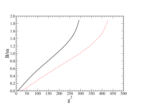
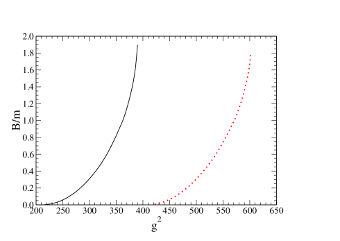
Figure 1: (color online) The binding energy $B/m$ vs $g^{2}$ for a scalar exchange (upper panel) and a pseudoscalar one (lower panel). In both cases, the vertex form-factor cutoff is $\Lambda/m=2$ (cf Eq. (3)). The masses of the exchanged scalar/pseudoscalar boson are $\mu/m=0.15$ (solid line) and $\mu/m=0.5$ (dotted line).

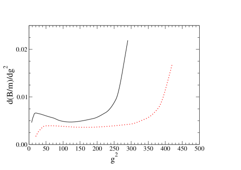
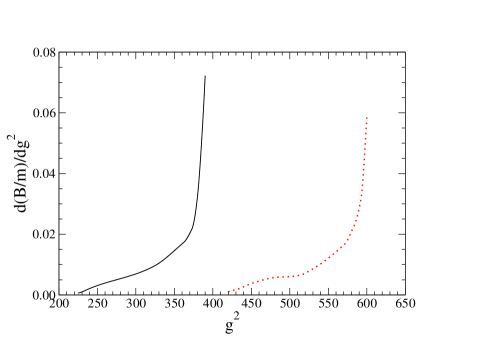
Figure 2: (color online) The same as in in Fig. 1, but for the corresponding derivatives $d(B/m)/dg^{2}$.

6.1 Binding energy vs Coupling Constants

We start by showing the binding energy $B/m$ as a function of $g^{2}$ for both scalar and pseudoscalar exchanges, fixing the cutoff in the vertex form factor, Eq. (3), to the value $\Lambda/m=2$. The results shown in Fig. 1, partially presented in Table I and II of Ref. dFSV1 , have been obtained by choosing the masses of the scalar and pseudoscalar exchanged bosons equal to $\mu/m=0.15$ and $\mu/m=0.50$. In particular, the lines shown in Fig. 1 allow one to illustrate interesting overall behaviors of the binding $B/m$, when the boson mass $\mu$ changes. In general, for fixed values of $\Lambda/m$ and $B/m$, the coupling constant $g^{2}$ increases as the mass of the exchanged boson increases. This feature is an expected one, if we take into account that the interaction has a range controlled by the inverse of $\mu$. Hence, if the range shrinks, then an increasing of the interaction strength is necessary for allocating a bound state with given $B/m$, as it is well-known also in the non relativistic case. In particular, for weakly bound systems, at fixed $B/m$, the correlation between the coupling constant $g^{2}$ and $\mu/m$ is almost linear (cf Tables I and II in Ref. dFSV1 for $B/m\leq 0.05$).

Moreover, the correlation between $g^{2}$ and $\mu$ is also driven by the nature of the exchanged boson, as shown by the quantitative differences illustrated in the upper and the lower panels in Fig. 1. As it is well-known in the non relativistic framework when the one-pion exchange is investigated, the pseudoscalar interaction is weak in a $0^{+}$ state. In particular, the tensor force obtained from the non relativistic reduction does not contribute in a $0^{+}$ state, and the remaining interaction gives a repulsive contribution, making impossible to bind the system. Only when the relativistic effects become important, the binding can be established, but for very large $g^{2}$ . In conclusion, in the pseudoscalar case, one is confronted with a much weaker attraction that requires, for a given binding energy, larger couplings than the scalar case needs.

When we approach the collapse of the bound state, i.e. when a composite massless particle is created since $B/m\to 2$, the shape of the binding becomes less sensitive to the variation of $g^{2}$ (a vertical asymptote is approached). By increasing the binding, the size of the system becomes smaller and smaller and therefore the range of the interaction, dictated by $\mu/m$, becomes less relevant for the functional dependence of the binding upon $g^{2}$ close to its critical value for $B/m=2$, namely the ultraviolet regime is now starting to govern the dynamics inside the system. This holds for both exchanges.

Let us now focus on the behavior of $d(B/m)/dg^{2}$, shown in Fig. 2. It is quite peculiar for the scalar case with respect to both pseudoscalar and vector cases (for the figure illustrating $B/m$ for the massless vector exchange see Ref. dFSV1 ), since it shows the presence of a minimum (less pronounced for $\mu/m=0.5$) positioned almost in the middle of the range of $g^{2}$ relevant for a given $\mu$. For the pseudoscalar case the minimum is close to the threshold, as a consequence of the repulsive contributions at low binding energies above mentioned. This observation suggests that also for the scalar case the appearance of a minimum be related to some repulsive contributions that develop for $B/m\to 2$ (i.e. $M\to 0$). As a matter of fact, from a direct inspection of Table 1, one can single out repulsive contributions that depends upon $1/M$.

6.2 Light-front amplitudes: Scalar case

The LF amplitudes $\psi_{i}(\gamma,\,\xi;\kappa^{2})$, Eq. (3.1), for the $0^{+}$ two-fermion system bound by a scalar exchange are presented in the Fig. 4. We compare two cases: weak binding $B/m=0.1$ (upper panels) and strong binding $B/m=1.0$ (lower panels). The motivation of such a comparison is given by the attempt of widening our intuition, based on non-relativistic physics, to the extreme binding, where the relativistic effects are expected to be relevant, like in the case of light pseudoscalar mesons. Indeed, in the present work an initial analysis of this physical case will be proposed by introducing and investigating a mock pion (see the next Sect. 7).

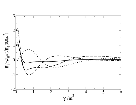
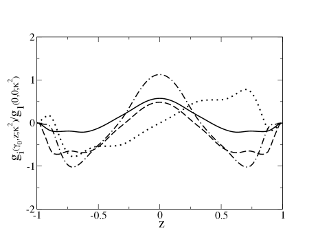
Figure 3: Nakanishi weight-functions $g_{i}(\gamma,\,z;\kappa^{2})$, Eqs. (12) and (13) evaluated for the $0^{+}$ two-fermion system with a scalar boson exchange such that $\mu/m=0.5$ and $B/m=0.1$ (the corresponding coupling is $g^{2}=52.817$ dFSV1 ). The vertex form-factor cutoff is $\Lambda/m=2$. Upper panel: $g_{i}(\gamma,\,z_{0};\kappa^{2})$ with $z_{0}=0.6$ and running $\gamma/m^{2}$. Lower panel: $g_{i}(\gamma_{0},\,z;\kappa^{2})$ with $\gamma_{0}/m^{2}=0.54$ and running $z$, The Nakanishi weight-functions are normalized with respect to $g_{1}(0,0;\kappa^{2})$. Solid line: $g_{1}$. Dashed line: $g_{2}$. Dotted line: $g_{3}$. Dot-dashed line: $g_{4}$.

To begin, it is useful to compare our results for the Nakanishi weight-functions with the outcomes obtained in Ref. CK2010 , within the Nakanishi framework, but inserting a smoothing function. In Fig. 3, the amplitudes $g_{i}(\gamma,z;\kappa^{2})$, corresponding to $\mu/m=0.5$ and $B/m=0.1$ (weak binding) as in Ref. CK2010 , are presented. The upper panel shows $g_{i}(\gamma,z;\kappa^{2})$ for a fixed values $z_{0}=0.6$ and running $\gamma$, while the lower panel illustrates the same quantities, but for $\gamma_{0}/m^{2}=0.54$ and running $z$. Recall that the results for the eigenvalues obtained in Ref. CK2010 coincide with ours (cf dFSV1 ) at the level of the published digits, while the eigenvectors, i.e. the Nakanishi weight-functions, are slightly different. Indeed, it is extremely encouraging to observe that so much different methods for taking into account the singularities in the BSE are able to achieve an overall agreement, (at least in weak-binding regime) in describing $g_{i}(\gamma,z;\kappa^{2})$, that have very rich structures.

In Fig. 4, results obtained with $\Lambda/m=2$ and $\mu/m=0.15$ are presented. It should be pointed out that the general behavior shown in Fig. 4 does not substantially change by increasing the mass of the exchanged boson up to $\mu/m=0.5$. Notice that the lhs of the figure contains $\psi_{i}(\gamma,\,\xi;\kappa^{2})$ for a fixed value of $\xi$ and running $\gamma$. The chosen value $\xi_{0}=0.2$ allows one to show in the same panel all the four $\psi_{i}$, since for $\xi=0.5$, where one should expect the maximal value (cf the rhs of the figure) $\psi_{3}$ vanishes. All the LF amplitudes are normalized to $\psi_{1}(\gamma=0,\xi=0.5)$, to quickly appreciate the relative strengths (in a forthcoming paper dFSV2 , it will be adopted the proper normalization through the BS amplitude for eventually obtaining the LF distributions).

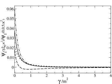
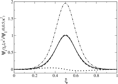
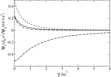
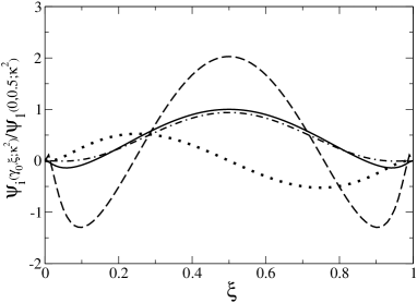
Figure 4: Light-front amplitudes $\psi_{i}(\gamma,\,\xi;\kappa^{2})$, Eq. (3.1), evaluated for the $0^{+}$ two-fermion system with a scalar boson exchange such that $\mu/m=0.15$. Upper panel: weak binding $B/m=0.1$ (the corresponding coupling is $g^{2}=23.12$ dFSV1 ). Lower panel: strong binding $B/m=1.0$ (the corresponding coupling is $g^{2}=187.8)$ dFSV1 ). The vertex form-factor cutoff is $\Lambda/m=2$. N.B. $\gamma_{0}=0$ and $\xi_{0}=0.2$ (see text). The LF distributions are normalized respect to $\psi_{1}(0,\xi=0.50;\kappa^{2})$. Solid line: $\psi_{1}$. Dashed line: $\psi_{2}$. Dotted line: $\psi_{3}$. Dot-dashed line: $\psi_{4}$.

The behavior for running $\gamma$ shows a difference between the weak and strong binding that can be directly ascribed to the size shrinking of the systems when the binding increases. Therefore the overall growing pattern of the amplitudes at higher $\gamma/m^{2}$ when $B/m$ increases (cf the lhs of Fig. 4 upper and lower panels) is an expected one. Remarkably, the characteristic momentum-width one can infer from the lines in Fig. 4 is of the order of $\gamma/m^{2}\sim B/m$. Another interesting feature is the growth of the amplitude $\psi_{2}$ when $B/m$ increases. This reflects the importance of singular terms in the ultraviolet region, since in this case one has the dominant role of the coefficient $c^{S}_{23}$ (see Eqs. (48) and (49) for counting the involved power of $k$). Already in Ref. CK2010 it was noted the strong singular contribution of the kernel at the end points when $c_{23}$ is nonzero, which is enhanced in the relativistic case of strong binding.

The dependence on $\xi$ of the LF amplitudes $\psi_{i}$ presented in rhs of Fig. 4 shows the expected peaks around 1/2, except for $\psi_{3}$, which is antisymmetric in $z$. Less trivial is the comparison between the weak- and strong-binding regime, in particular for $\psi_{2}$ and $\psi_{4}$. It can be seen that for $B/m=1$, the LF amplitude $\psi_{2}$ accumulates toward the end points, a property which seems to be slightly present also in $\psi_{1}$. This feature can be traced to the same effect seen for running $\gamma$, namely the relevance of the coefficient $c^{S}_{23}$, associated to the singular behavior at the end points. For the weak binding case, the effect is damped, as one could naively guess from the observation that $|\vec{k}|$ and $|\vec{k}^{\prime}|$ are of the order of $B\ll m$ (cf the upper left panel) and $c^{S}_{23}\sim B^{3}/M$, while for example $c^{S}_{21}=m\,M$. Noteworthy $\psi_{4}$, driving the spin-momentum correlation, appears to be maximal for a weakly bound system for $\gamma=0$ in a state $0^{+}$. The prominence of this component can be explained by considering the first two coefficients, $c^{S}_{14}$ and $c^{S}_{24}$ (see Eqs. (48) and (49)) that are proportional to $M^{2}$ and $M$ respectively. By comparing those coefficient with the corresponding $c^{S}_{11}$ and $c^{S}_{22}$ one can roughly understand the factor of two between $\psi_{4}$ and $\psi_{2}$ at the peak $\xi=0.5$ for weak binding. The same relevance of the $\psi_{4}$ component can be found for both the pseudoscalar and vector exchange (see below). In particular, this last case leads us to focus the previous discussion on the coefficients by excluding $c^{S}_{44}$, since $c^{V}_{44}=0$ but the effect is present. Moreover, given the smallness of $\psi_{3}$ one can pay attention only on $c^{S}_{14}$ and $c^{S}_{24}$.

As a final remark, one should notice in the rhs that the LF amplitudes enlarge their-own range when $B/m$ grows, as expected from the size shrinking of the system.

6.3 Light-front amplitudes: Pseudoscalar case

The general comments, with a particular emphasis on the relevance of the coefficients producing LF singularities, presented for the scalar case are suitable also for the LF amplitudes $\psi_{i}(\gamma,\,\xi;\kappa^{2})$ obtained by using a pseudoscalar exchange with $\mu/m=0.15$. But, a crucial difference is generated by the peculiar dynamics entailed by the spinor coupling characterizing the two cases, as already pointed out for Fig. 1. Such a difference plays a role in explaining the leading position of $\psi_{4}$, that is related to the spin-momentum correlations.

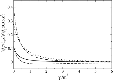
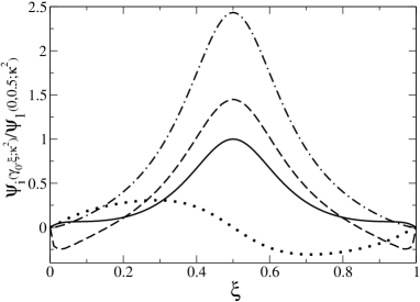
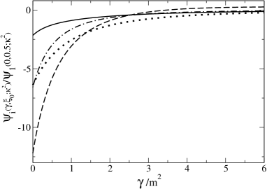
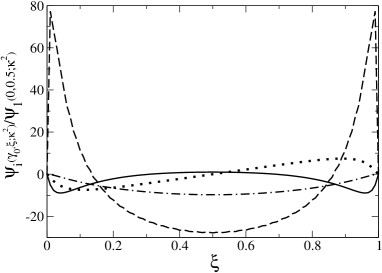
Figure 5: Light-front amplitudes $\psi_{i}(\gamma,\,\xi;\kappa^{2})$, Eq. (3.1), evaluated for the $0^{+}$ two-fermion system with a pseudoscalar boson exchange such that $\mu/m=0.15$. Upper panels: weak binding $B/m=0.1$ (the corresponding coupling is $g^{2}=262.1$ dFSV1 ). Lower panels: strong binding $B/m=1.0$ (the corresponding coupling is $g^{2}=362.3)$ dFSV1 ). The vertex form-factor cutoff is $\Lambda/m=2$. N.B. $\gamma_{0}=0$ and $\xi_{0}=0.2$ (see text). Solid line: $\psi_{1}$. Dashed line: $\psi_{2}$. Dotted line: $\psi_{3}$. Dot-dashed line: $\psi_{4}$.

The dependence of $\psi_{i}$ on $\xi$ is presented in the right panels of Fig. 5. For the weakly bound case, one notices that $\psi_{1}$ and $\psi_{2}$ are somewhat different while in the scalar case they almost coincide. We trace back the reason for that, by looking at the spinor structure associated to each $\psi_{i}$. The Dirac operator for $\psi_{1}$ is $\gamma_{5}$ and for $\psi_{2}$ is $/\!\!\!{p}\gamma_{5}/M$. For both cases in the weak binding limit, namely in the non-relativistic regime, the vector charge and scalar charge densities of the state are expected to be close, and in the scalar coupling case the corresponding operators commutes with the scalar coupling Dirac operator. For the pseudoscalar case, the $\gamma_{5}$ coupling has opposite commutation properties with the Dirac structure associated to $\psi_{1}$ and $\psi_{2}$, and this feature can be identified as the source for the observed difference in the upper-left panel of Fig. 5.

In conclusion, the performed analysis of scalar and pseudoscalar exchanges yields a description coherent with the intuition stemming from the general structure of both the BS amplitude and the kernel, and increases the confidence in the novel approach we are pursuing for solving BSE in Minkowski space. Therefore, to address the vector exchange with such a reliable tool becomes a very stimulating issue, given its possible application to hadron physics.

6.4 Light-front amplitudes: Vector case

Starting from the solution of the four-dimensional BSE, our goal is to construct a phenomenological tool for analyzing the structure of a simple model of the pion, namely a quark-antiquark pair living in Minkowski space and bound through a massive vector exchange.

Table 2: The vector coupling vs the binding energy for a massless vector exchange, i.e. $\mu/m=0$. First column: binding energy. Second column: coupling constant $g^{2}$, obtained by taking analytically into account the fermionic singularities, (see text). Third column: results obtained in Ref. CK2010 where the singularities are treated numerically, by using a smoothing function. The vertex form factor cutoff is $\Lambda/m=2$.

B/m	$g^{2}_{dFSV}$(full)	$g^{2}_{CK}$
0.01	3.273	3.265
0.02	4.913	4.910
0.03	6.261	6.263
0.04	7.454	7.457
0.05	8.548	8.548
0.10	13.15	13.15
0.20	20.43	20.43
0.30	26.51	26.50
0.40	31.86	31.84
0.50	36.66	36.62
1.00	54.62	-
1.20	59.51	-
1.40	63.23	-
1.60	65.86	-
1.80	67.43	-

Before considering a quark-antiquark system, we continue our analysis of the changes in the structure of the $0^{+}$ state with different couplings and binding energies in order to fully appreciate the subtleties generated by the dynamics inside the bound state. It is worth bearing in mind how accurate are our calculations by presenting a quantitative comparison with analogous calculations shown in Ref. CK2010 . The massless exchange between two fermions in the $0^{+}$ state was considered (i.e. Eq. (6) with $\mu^{2}=0$). As shown in Table 2, the agreement is excellent, and moreover the possibility to have a formal treatment of the LF singularities allows us to extend the range of the calculations. The behavior of $B/m$ as a function of $g^{2}$ (see the corresponding figure in dFSV1 ) has the same overall structure found for the pseudoscalar case, with a minimum of the derivative of $d(B/m)/dg^{2}$ close to the threshold.

Given that, before treating the mock pion problem, we present results for a massive vector with $\mu/m=0.15$, still using the form factor parameter equal to $\Lambda/m=\,2$. As it is easily seen, in Fig. 6 general patterns similar to the ones observed for the pseudoscalar case can be recognized, when one moves from weak- to strong-binding regime.

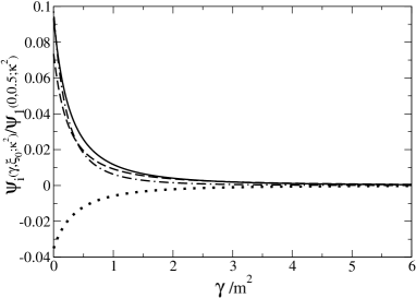
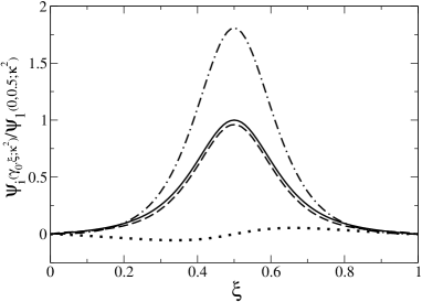
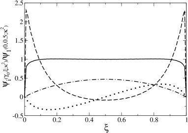
Figure 6: Light-front amplitudes $\psi_{i}(\gamma,\,\xi;\kappa^{2})$, Eq. (3.1), evaluated for the $0^{+}$ two-fermion system with a massive vector exchange such that $\mu/m=0.15$. Upper panel: weak binding $B/m=0.1$ (the corresponding coupling is $g^{2}=16.65$). Lower panel: strong binding $B/m=1.0$ (the corresponding coupling is $g^{2}=59.23)$). The vertex form-factor cutoff is $\Lambda/m=2$. N.B. $\gamma_{0}=0$ and $\xi_{0}=0.2$ (see text). Solid line: $\psi_{1}$. Dashed line: $\psi_{2}$. Dotted line: $\psi_{3}$. Dot-dashed line: $\psi_{4}$.

The dependence of the LF amplitudes $\psi_{1}$ and $\psi_{2}$ on $\xi$, in the right panels of the figures, suffers a dramatic change from weak to strong binding, while the amplitudes $\psi_{3}$ and $\psi_{4}$ just get wider when the binding increases (apart the change of sign of $\psi_{3}$). As in the scalar case, the amplitudes $\psi_{1}$ and $\psi_{2}$ almost coincide for running $\xi$ and $\gamma=0$, in the weak binding case. This feature can be understood by considering the Dirac structure associated with $\psi_{1}$ and $\psi_{2}$ in the expansion of the BS amplitude, i.e. $\gamma_{5}$ for the first amplitude and $\gamma_{0}\gamma_{5}$ for the second one, in the CM frame. In the non relativistic limit, the vector interaction largely reduces to its Coulomb component, whose Dirac structure, $\gamma_{0}$, has equal commutation properties with the ones associated to $\psi_{1}$ and $\psi_{2}$. The same happens when the scalar exchange is considered, since one has simply the identity matrix at the interaction vertex. Moreover, in the weak binding regime, the scalar and charge densities of the fermionic constituents (acting at the interaction vertices) tend to be the same, while for growing $B/m$ this is not the case. Finally, notice that even the coupling constants $g^{2}$ are similar for scalar and vector exchange, in the weak binding regime.

Moving from weak to strong binding the amplitudes $\psi_{1}$, $\psi_{3}$ and $\psi_{4}$ become wider as a function of $\xi$. A new feature arises in $\psi_{1}$, it becomes quite flat and sharply decreasing at the end points, while $\psi_{2}$ has the characteristic peaks discussed before. The flattening of $\psi_{1}$ appears to be a signature of the vector coupling, since it remains present when the vector mass increases, as illustrated in the next Section. Indeed, all the patterns shown in Fig. 6 do not qualitatively change when the mass of the exchanged boson grows.

7 The mock pion

In this Section, we present a first investigation of a simplified model for the pion, that, at some extent, can be considered Lattice-QCD inspired. In particular, we have tuned our parameters, like the masses of quark and exchanged vector boson, according to the outcomes of Lattice-QCD calculations.

As above illustrated, within the formal elaboration one adopts for getting solutions of BSE, it is natural to switch to a BS amplitude pertaining to a fermion-antifermion system. If one multiplies the original fermion-fermion BS amplitude by the charge-conjugation operator, then one gets a compact expression of the BSE with fermionic degrees of freedom, eventually using the standard multiplication rule for matrices. Summarizing, the scalar functions (Eq. (7)) that enter both fermion-fermion ($0^{+}$) and fermion-antifermion ($0^{-}$) BS amplitudes are the same, but the Dirac structures are different, as it must be. The ladder kernel we exploit is the one corresponding to a massive vector exchange, in Feynman gauge (cf Eq. (6)), with the same vertex form factor in Eq. (3).

Table 3: Coupling constants for our Lattice-QCD inspired mock pion, obtained with $B/m=1.44$ and $\mu/m=2.0$. Two values for vertex form factor cutoff $\Lambda/m$, have been chosen.

$\Lambda/m$	$g^{2}$	$\alpha_{s}$ Eq. (47)
3	435.0	10.68
8	52.0	3.71

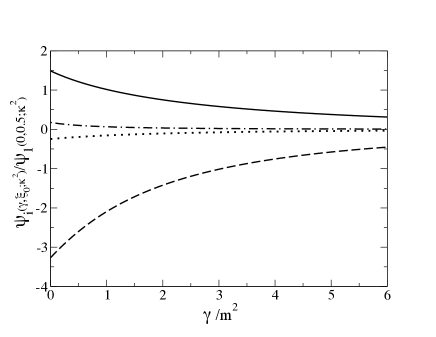
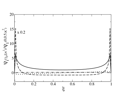
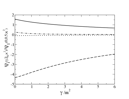
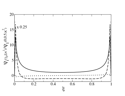
Figure 7: Light-front amplitudes $\psi_{i}(\gamma,\,\xi;\kappa^{2})$, Eq. (3.1), for the pion-like system with a heavy-vector exchange $(\mu/m=2)$, binding energy of $B/m=1.44$ and constituent mass $m=250$ MeV. Upper panel: vertex form-factor cutoff $\Lambda/m=3$ and $g^{2}=435.0$, corresponding to $\alpha_{s}=10.68$ (see text for the definition of $\alpha_{s}$). Lower panel: vertex form-factor cutoff $\Lambda/m=8$ and $g^{2}=53.0$, corresponding to $\alpha_{s}=3.71$. The value of the longitudinal variable is $\xi_{0}=0.2$ and $\gamma_{0}=0$ . Solid line: $\psi_{1}$ . Dashed line: $\psi_{2}$. Dotted line: $\psi_{3}$. Dot-dashed line: $\psi_{4}$

Lattice-QCD results obtained in Refs OLJPG11 ; DuaPRD16 ; OliFBS17 , by adopting the Landau gauge, indicate that the gluon propagator obtained in the space-like region is infrared finite and can be roughly described by using a massive propagator with a dynamical gluon mass $\mu\sim 500$ MeV. For the moment, we assume such a handy approximation for the gluon propagator which is able to qualitatively incorporate the relevant momentum scale, but in the Feynman gauge (see Eq. (6)). Moreover, Ref. ParPRD06 suggests for the lattice quark propagator a dynamical mass $m\sim 250$ MeV, at zero momentum. In conclusion, we have adopted i) a pion mass of about 140 MeV leading to a binding energy $B/m=1.44$ (recall that $M=2m-B$), ii) a mass for the exchanged vector $\mu/m=2$, and iii) a cutoff in the vertex form factor $\Lambda/m$. For such a quantity, we have chosen two values, $\Lambda/m=3$ and $\Lambda/m=8$, that correspond to a size of the interaction vertex less than the range of the interaction itself, and, according to Fig. 5.3 of Ref. Deur:2016tte , yield a reasonable rescaled coupling constant in the infrared region. What we call rescaled coupling constant, to stress the difference with $g^{2}$, is defined by (cf the vertex form factors in Eqs. (4.1) and (39) as well as Eq. (43))

$$\alpha_{s}={g^{2}\over 4\pi}~{}\left(1-{\mu^{2}\over\Lambda^{2}}\right)^{2}~{}~{}.$$ (47)

Finally, it is worth noticing that the assumed value of the constituent mass gives a binding energy $B=1.44~{}m=360$ MeV, that leads to a typical size of $\hbar\,c/B=$ 0.55 fm, quite close to the experimental pion charge radius of 0.672$\pm$0.008 fm pdg .

The eigenvalues $g^{2}$, obtained with the above set of parameters, and the corresponding $\alpha_{s}$ are summarized in Table 3, while the LF amplitudes of our mock pion, are presented in Fig. 7. It is possible to recognize an overall behavior of the $\psi_{i}$’s similar to the one in Fig. 6, where a strong-binding case $B/m=1$ for a vector exchange with $\mu/m=0.15$ and $\Lambda/m=2$ is shown. But it is much more interesting to observe the effects produced by varying exchanged mass $\mu/m$ and vertex cutoff $\Lambda/m$. As $\mu/m$ increases the tails of the LF amplitudes do the same (cf lhs of Figs. 6 and 7): given the overall size of the system (fixed by the binding energy), one has a reduction of the interaction range, that in turn triggers a shrinking of the system itself. The same kind of effect can be seen also decreasing the size of the interaction vertex, i.e. by increasing $\Lambda/m$. More striking is the effect shown in the rhs of Fig. 7, where the LF amplitudes are given as a function of the variable $\xi$. There, one can observe a quite peculiar two-horn pattern, that becomes more enhanced when $\Lambda/m$ grows. The striking two-horn pattern are due to the presence of spin degrees of freedom (see, the differences with the case of a two-scalar system in Ref. FSV2 ). Bearing in mind that we will investigate such structures in a forthcoming paper dFSV2 , we expect non trivial impacts of the above feature on the evaluation of both TMDs (see e.g. lorce2015unpolarized ) and valence distributions (that contain a multiplicative factor $\xi(1-\xi)$). In view of this, it is suggestive to recall a well-known pion distribution amplitude introduced in Ref. Chernyak:1981zz that displays a two-horn pattern.

8 Conclusions and summary

In the present paper, we have described in great detail our approach for getting actual solutions, directly in Minkowski space, of the ladder Bethe-Salpeter equation for a system of two interacting fermions, in a state $0^{+}$, as well as a fermion-antifermion system in $0^{-}$ channel. This effort makes complete the presentation of our approach, shortly illustrated in Ref. dFSV1 , where the most urgent aim was the quantitative comparison with the eigenvalues obtained in Ref. CK2010 and in the Euclidean space Dork . The large amount of provided information allows one to assess in depth the approach based on the Nakanishi integral representation of the BS amplitude. Hence, one can easily recognize that the approach is a very effective tool for exploring the non perturbative dynamics inside a relativistic system, since it combines flexibility (one is able to address higher-spin system) and feasibility of affordable calculations.

The main ingredients for proceeding toward the numerical solution of the coupled system of integral equations, formally equivalent to the initial BSE, are i) the Nakanishi integral representation of the BS amplitude and ii) the LF-projection of the BS amplitude, that allows one to get LF amplitudes depending upon real variables. In order to embed the approach based on NIR into a well-defined mathematical framework, it is fundamental to notice that those LF distributions have exactly the form of a general Stieltjes transform Carbonell:2017kqa , and therefore the NIR approach appears to be more general than one could suspect from the Nakanishi work focused on the diagrammatic analysis of the transition amplitudes nak63 ; nak71 . The analysis of the Stieltjes transform method for investigating the fermionic BSE will be left to future work. Moreover, the LF projection plays also a key-role in determining the LF singularities that, in principle, plague the method (as shown in Ref. CK2010 , where a function was introduced for smoothing the singular behavior of the involved kernel). In particular, by exploiting previous analyses of the LF singularities Yan , we succeeded in formally treating them. As a consequence, we have obtained calculable matrix elements, after introducing an orthonormal basis for expanding the four Nakanishi weight functions needed for achieving the description of the fermionic states (for a $1^{+}$ states the weights become eight).

We have shown and discussed both eigenvalues and eigenvectors of the generalized eigenvalue problem one gets after inserting in the BSE three different kernels, featuring massive scalar, pseudoscalar and vector exchanges. Such interactions produce very peculiar form for the correlation between the binding energy and the coupling constant $g^{2}$. From the eigenvectors, i.e. the Nakanishi weight-functions, we have evaluated the corresponding LF amplitudes, that show the effects of the exchange in action. It should be recalled that the LF amplitudes are the building-blocks for constructing transverse-momentum distributions and valence wave functions (see, e.g. FSV1 ; FSV2 ). Last but not least, we have presented the application to a simplified model of the pion, by taking the mass of the constituents and the mass of the exchanged vector boson (with a Feynman-gauge propagator) from some typical lattice calculations. The intriguing feature shown in the rhs of Fig. 7 will be furtherly discussed in Ref. dFSV2 , where also the transverse-momentum distributions of a $0^{-}$ state will be investigated.

In conclusion, we would like to emphasize that the present approach can be certainly enriched with new features impacting both kernel and self-energies of both constituents and intermediate boson, but already at the present exploratory stage it appears to have a great potentiality, as a phenomenological tool for facing with strongly relativistic systems, in Minkowski space.

Appendix A The coefficients $c_{ij}$

In this Appendix, the coefficients $c_{ij}$ in Eq. (10) that determine the kernel of the BSE for scalar, pseudoscalar and vector exchanges, are briefly discussed. For the scalar exchange, one has

$$c^{S}_{11}=m^{2}+\frac{M^{2}}{4}-k^{2},\,c^{S}_{12}=mM,\,c^{S}_{14}=-{B^{\prime}\over M^{2}},$$

$$c^{S}_{21}=mM,~{}~{}c^{S}_{22}=m^{2}+\frac{M^{2}}{4}+k^{2}-2\frac{(p\cdot k)^{2}}{M^{2}},$$

$$c^{S}_{23}=-2{B^{\prime}\over M^{4}}(p\cdot k),\,c^{S}_{24}=-2B^{\prime}{m\over M^{3}},$$

$$c^{S}_{32}=2(p\cdot k),c^{S}_{33}=\frac{B^{\prime}}{B}\left(m^{2}-\frac{M^{2}}{4}+2\frac{(p\cdot k)^{2}}{M^{2}}-k^{2}\right),\,$$

$$c^{S}_{34}=2\frac{B^{\prime}}{B}\frac{m}{M}(p\cdot k),c^{S}_{41}=M^{2},~{}~{}c^{S}_{42}=2mM,$$

$$c^{S}_{43}=2\frac{B^{\prime}}{B}\frac{m}{M}(p\cdot k),~{}~{}c^{S}_{44}=-\frac{B^{\prime}}{B}\left(\frac{M^{2}}{4}-m^{2}-k^{2}\right),$$

(48)

with $c^{S}_{13}=c^{S}_{31}=0$, $B$ and $B^{\prime}$ defined by

$$B=(p\cdot k)^{2}-M^{2}k^{2}\,$$

$$B^{\prime}=(p\cdot k)(p\cdot k^{\prime\prime})-M^{2}(k\cdot k^{\prime\prime})~{}.$$ (49)

The other two sets of coefficients can be obtained from $c^{S}_{ij}$ by exploiting the properties of the Dirac matrices. In particular, one gets for the pseudoscalar exchange

$$c_{i1}^{PS}=-c_{i1}^{S},\quad c_{i2}^{PS}=c_{i2}^{S},\quad c_{i3}^{PS}=c_{i3}^{S},$$

$$c_{i4}^{PS}=-c_{i4}^{S},~{}\forall i~{}.$$

and for the vector exchange

$$c_{i1}^{V}=4~{}c_{i1}^{S},\quad c_{i2}^{V}=-2~{}c_{i2}^{S},\quad c_{i3}^{V}=-2~{}c_{i3}^{S},$$

$$c_{i4}^{V}=0,~{}\forall i~{}.$$

(51)

For carrying out the discussion of the LF singularities one meets, it is useful to decompose the coefficients $c_{ij}(k,k^{\prime\prime},p)$ so that terms with the same power of $k^{\mu}$ are gathered together. Namely

$$c^{S}_{ij}(k,k^{\prime\prime},p)=a^{0}_{ij}+a^{1}_{ij}~{}(p\cdot k)+a^{2}_{ij}~{}(p\cdot k)^{2}$$

$$+a^{3}_{ij}~{}k^{2}+{1\over B}\Bigl{[}(p\cdot k)(p\cdot k^{\prime\prime})-M^{2}(k\cdot k^{\prime\prime})\Bigr{]}$$

$$\times\Bigl{[}b^{0}_{ij}+b^{1}_{ij}~{}(p\cdot k)+b^{2}_{ij}~{}(p\cdot k)^{2}+b^{3}_{ij}~{}k^{2}\Bigr{]}$$

$$+\Bigl{[}(p\cdot k)(p\cdot k^{\prime\prime})-M^{2}(k\cdot k^{\prime\prime})\Bigr{]}$$

$$\times~{}\Bigl{[}d^{0}_{ij}+d^{1}_{i,j}~{}(p\cdot k)\Bigr{]},$$ (52)

where the non vanishing coefficients $a^{n}_{ij}$, $b^{n}_{ij}$ and $d^{n}_{ij}$ are given by

$$a_{11}^{0}=m^{2}+M^{2}/4\,,a_{12}^{0}=mM\,,a_{21}^{0}=mM\,,$$

$$a_{22}^{0}=m^{2}+M^{2}/4\,,a_{41}^{0}=M^{2}\,,a_{42}^{0}=2mM\,,a_{32}^{1}=2\,,$$

$$a_{22}^{2}=-2/M^{2}\,,a_{11}^{3}=-1\,,a_{22}^{3}=1\,,$$

$$b_{33}^{0}=m^{2}-M^{2}/4\,,b_{34}^{1}=2m/M\,,b_{43}^{1}=2m/M\,,$$

$$b_{44}^{1}=m^{2}-M^{2}/4\,,b_{33}^{2}=2/M^{2}\,,b_{33}^{3}=-1\,,$$

$$d_{14}^{0}=-1/M^{2}\,,d_{24}^{0}=-2m/M^{3}\,,d_{44}^{0}=1\,,d_{23}^{1}=-2/M^{4}\,.$$

(53)

Appendix B Analytic integration on $k^{-}$ of the kernel ${\cal L}_{ij}$ for any $k^{+}_{D}$

This Appendix contains the details on the integration in the complex $k^{-}$-plane of the kernel ${\cal L}_{ij}$, Eq. (25), for any value of $k^{+}_{D}$. Namely, we obtain the general expression of the coefficients ${\cal C}_{n}$ defined in Eq. (26). They are necessary for determining the kernel ${\cal L}_{ij}$.

One can write

$${\cal C}_{n}=~{}-{\partial\over\partial\ell_{D}}{\cal B}_{n}$$ (54)

where $n=0,1,2,3$ and

$${\cal B}_{n}=2\int{dk^{-}\over 2\pi}~{}{(k^{-})^{n}~{}\over\Bigl{[}(1-z)(k^{-}-k^{-}_{d})+i\epsilon\Bigr{]}}$$

$$\times~{}{1\over\Bigl{[}(1+z)(k^{-}-k^{-}_{u})-i\epsilon\Bigr{]}}$$

$$\times\int^{1}_{0}d\xi_{1}~{}{\xi_{1}\over\Bigl{[}k^{+}_{D}k^{-}+\ell_{D}+\xi_{1}(1-v)\Bigl{(}\mu^{2}-\Lambda^{2}\Bigr{)}+i\epsilon\Bigr{]}^{3}}$$

where it has been applied the Feynman trick to the denominators containing $k^{+}_{D}$ for obtaining the final expression.

The issue is the possibility or not to apply the Cauchy’s residue theorem for getting an analytic result. Hence, one has to carefully check if the arc at infinity gives or not a vanishing contribution. As it is shown in what follows, a positive answer depends upon the values of $n$ and $k^{+}_{D}$.

The $n=0$ case is not affected by any difficulty due to values of $k^{+}_{D}$. One can always close the arc at infinity, even for $k^{+}_{D}=0$. Indeed, if the last case happens, one could be concerned about the end-points $z=\pm 1$, but, fortunately, one remains with a standard LF integration and gets a finite result (see Ref. bakker2005restoring ). The evaluation of ${\cal B}_{0}$ proceeds by exploiting the residue theorem, obtaining

$${\cal B}_{0}={i\Bigl{[}\theta(k^{+}_{D})~{}{\cal I}(k^{-}_{u})+\theta(-k^{+}_{D})~{}{\cal I}(k^{-}_{d})\Bigl{]}\over(1-z^{2})~{}(k^{-}_{u}-k^{-}_{d})}~{},$$ (56)

where

$${\cal I}(k^{-}_{u})={1\over\Bigl{[}k^{+}_{D}k^{-}_{u}+\ell_{D}+(1-v)\Bigl{(}\mu^{2}-\Lambda^{2}\Bigr{)}+i\epsilon\Bigr{]}^{2}}$$

$$\times~{}{1\over\Bigl{[}k^{+}_{D}k^{-}_{u}+\ell_{D}+i\epsilon\Bigr{]}}$$ (57)

and the analogous expression for ${\cal I}(k^{-}_{d})$. Then ${\cal C}_{0}$ is given by

$${\cal C}_{0}=-{i\over(1-z^{2})~{}(k^{-}_{u}-k^{-}_{d})}$$

$$\times~{}\left[\theta(k^{+}_{D})~{}{\partial\over\partial\ell_{D}}{\cal I}(k^{-}_{u})++\theta(-k^{+}_{D})~{}{\partial\over\partial\ell_{D}}{\cal I}(k^{-}_{d})\right]~{}.$$ (58)

For $n=1$, the integral ${\cal B}_{1}$ is

$${\cal B}_{1}=I_{1}+k^{-}_{u}{\cal B}_{0}$$ (59)

with

$$I_{1}=-{2i\over(1-z^{2})}\theta(-k^{+}_{D})~{}\int_{0}^{1}d\xi_{1}~{}\xi_{1}$$

$$\times~{}{1_{1}\over\Bigl{\{}k^{+}_{D}k^{-}_{d}+\ell_{D}+\xi_{1}(1-v)\Bigl{(}\mu^{2}-\Lambda^{2}\Bigr{)}+i\epsilon\Bigr{\}}^{3}}~{}.$$

Let us remind that $-(1-z)M/(k^{+}_{D}-(1-z)M)\geq 0$ for $0\geq k^{+}_{D}$.

Summarizing, one gets

$${\cal B}_{1}={i\Bigl{[}k^{-}_{u}\theta(k^{+}_{D})~{}{\cal I}(k^{-}_{u})+k^{-}_{d}\theta(-k^{+}_{D})~{}{\cal I}(k^{-}_{d})\Bigr{]}\over(1-z^{2})(k^{-}_{u}-k^{-}_{d})}~{}.$$

Then ${\cal C}_{1}$ is given by

$${\cal C}_{1}=-{i\over(1-z^{2})(k^{-}_{u}-k^{-}_{d})}$$

$$\times~{}\left[k^{-}_{u}~{}\theta(k^{+}_{D})~{}{\partial\over\partial\ell_{D}}{\cal I}(k^{-}_{u})+k^{-}_{d}~{}\theta(-k^{+}_{D})~{}{\partial\over\partial\ell_{D}}{\cal I}(k^{-}_{d})\right]~{}.$$

For $n=2$, the integral ${\cal B}_{2}$ is

$${\cal B}_{2}={i\,\delta(k^{+}_{D})\over(1-z^{2})\Bigl{[}(1-v)\Bigl{(}\mu^{2}-\Lambda^{2}\Bigr{)}\Bigr{]}^{2}}$$

$$\times~{}\left[{(1-v)\Bigl{(}\mu^{2}-\Lambda^{2}\Bigr{)}\over\Bigl{[}\ell_{D}+(1-v)\Bigl{(}\mu^{2}-\Lambda^{2}\Bigr{)}+i\epsilon\Bigr{]}}-L(\ell_{D})\right]$$

$$+{i\Bigl{[}(k^{-}_{u})^{2}\theta(k^{+}_{D})~{}{\cal I}(k^{-}_{u})+(k^{-}_{d})^{2}\theta(-k^{+}_{D})~{}{\cal I}(k^{-}_{d})\Bigr{]}\over(1-z^{2})(k^{-}_{u}-k^{-}_{d})}~{}.$$

where

$$L(\ell_{D})=\ln\left({\ell_{D}+(1-v)\Bigl{(}\mu^{2}-\Lambda^{2}\Bigr{)}\over\ell_{D}}\right)$$ (64)

Then, ${\cal C}_{2}$ is given by the sum of a singular term and the non singular one already obtained, i.e.

$${\cal C}_{2}=-{i\over(1-z^{2})}~{}{\delta(k^{+}_{D})~{}\over\ell_{D}\Bigl{[}\ell_{D}+(1-v)\Bigl{(}\mu^{2}-\Lambda^{2}\Bigr{)}+i\epsilon\Bigr{]}^{2}}~{}$$

$$-{i\over(1-z^{2})(k^{-}_{u}-k^{-}_{d})}~{}\Bigl{[}(k^{-}_{u})^{2}\theta(k^{+}_{D})~{}{\partial\over\partial\ell_{D}}{\cal I}(k^{-}_{u})$$

$$+(k^{-}_{d})^{2}\theta(-k^{+}_{D})~{}{\partial\over\partial\ell_{D}}{\cal I}(k^{-}_{d})\Bigr{]}$$ (65)

For $n=3$, the integral ${\cal B}_{3}$ is

$${\cal B}_{3}=~{}{i\over(1-z^{2})}~{}{\partial\over\partial k^{+}_{D}}\delta(k^{+}_{D})~{}{1\over\Bigl{[}(1-v)\Bigl{(}\mu^{2}-\Lambda^{2}\Bigr{)}\Bigr{]}^{2}}$$

$$\times~{}\left[(1-v)\Bigl{(}\mu^{2}-\Lambda^{2}\Bigr{)}-\ell_{D}~{}L(\ell_{D})\right]$$

$$+(k^{-}_{u}+k^{-}_{d})~{}{\cal B}_{2}-k^{-}_{u}k^{-}_{d}~{}{\cal B}_{1}$$

Then ${\cal C}_{3}$ contains both singular and non singular contributions as in the case of ${\cal C}_{2}$. One has

$${\cal C}_{3}={i\over(1-z^{2})}~{}{\partial\over\partial k^{+}_{D}}\delta(k^{+}_{D})~{}{1\over\Bigl{[}(1-v)\Bigl{(}\mu^{2}-\Lambda^{2}\Bigr{)}\Bigr{]}^{2}}$$

$$\times~{}\left[L(\ell_{D})-{{(1-v)}(\mu^{2}-\Lambda^{2})\over\ell_{D}+{(1-v)}(\mu^{2}-\Lambda^{2})}\right]$$

$$-{i~{}(k^{-}_{u}+k^{-}_{d})\over(1-z^{2})}~{}{\delta(k^{+}_{D})~{}\over\ell_{D}\Bigl{[}\ell_{D}+(1-v)\Bigl{(}\mu^{2}-\Lambda^{2}\Bigr{)}+i\epsilon\Bigr{]}^{2}}~{}$$

$$-{i\over(1-z^{2})(k^{-}_{u}-k^{-}_{d})}~{}\Bigl{[}(k^{-}_{u})^{3}\theta(k^{+}_{D})~{}{\partial\over\partial\ell_{D}}{\cal I}(k^{-}_{u})$$

$$+(k^{-}_{d})^{3}\theta(-k^{+}_{D})~{}{\partial\over\partial\ell_{D}}{\cal I}(k^{-}_{d})\Bigr{]}$$ (67)

Appendix C Singular terms for scalar, pseudoscalar and vector interactions

In this Appendix, the final expressions of the singular contributions obtained in the previous B are explicitly given, in order to facilitate a quick usage of the main results of our work. For the scalar case, the non vanishing contributions for the singular part of ${\cal L}^{(s)}_{ij}$ are

$${\cal L}^{(s)}_{14}={i\over M}~{}{(\mu^{2}-\Lambda^{2})^{2}\over 8\pi^{2}M^{2}}~{}{\delta(z^{\prime}-z)\over 2(1-z^{2})}\int^{1}_{0}dv~{}{v~{}(1-v)^{2}\over D_{\ell}}$$

$${\cal L}^{(s)}_{22}={i\over M}~{}{(\mu^{2}-\Lambda^{2})^{2}\over 8\pi^{2}M^{2}}~{}{\delta(z^{\prime}-z)\over(1-z^{2})}\int^{1}_{0}dv~{}{v~{}(1-v)\over D_{\ell}}$$

$${\cal L}^{(s)}_{24}={i\over M}~{}{(\mu^{2}-\Lambda^{2})^{2}\over 8\pi^{2}M^{2}}~{}{m\over M}~{}{\delta(z^{\prime}-z)\over(1-z^{2})}\int^{1}_{0}dv~{}{v~{}(1-v)^{2}\over D_{\ell}}$$

$${\cal L}^{(s)}_{33}=-{i\over M}~{}{(\mu^{2}-\Lambda^{2})^{2}\over 8\pi^{2}M^{2}}~{}{\delta(z^{\prime}-z)\over(1-z^{2})}\int^{1}_{0}dv~{}{v~{}(1-v)^{2}\over D_{\ell}}$$

$${\cal L}^{(s)}_{23}={\cal L}^{(s)}_{23}(a)+{\cal L}^{(s)}_{23}(b)$$ (68)

with

$${\cal L}^{(s)}_{23}(a)={i\over M}~{}{(\mu^{2}-\Lambda^{2})^{2}\over 8\pi^{2}M^{2}}~{}\delta(z^{\prime}-z)~{}{2z\over M^{2}(1-z^{2})^{2}}$$

$$\times\Bigl{[}{M^{2}~{}(1-z^{2})\over 8}+\gamma+m^{2}\Bigr{]}\int^{1}_{0}dv~{}{v~{}(1-v)^{2}\over D_{\ell}}$$ (69)

$${\cal L}^{(s)}_{23}(b)={i\over M}~{}{1\over 8\pi^{2}M^{4}~{}(1-z^{2})}~{}\Bigl{[}{\partial\over\partial z^{\prime}}\delta(z^{\prime}-z)\Bigr{]}$$

$$\times\int^{1}_{0}dv~{}{1\over(1-v)}~{}\left[{(1-v)\Bigl{(}\mu^{2}-\Lambda^{2}\Bigr{)}\over\ell_{D}+(1-v)\Bigl{(}\mu^{2}-\Lambda^{2}\Bigr{)}}-L(\ell_{D})\right]$$

(70)

In the above expressions

$$D_{\ell}=\tilde{\ell}_{D}\Bigl{[}\tilde{\ell}_{D}+(1-v)\Bigl{(}\mu^{2}-\Lambda^{2}\Bigr{)}+i\epsilon\Bigr{]}^{2}$$

$$\tilde{\ell}_{D}=-v(1-v)~{}\gamma-v\Bigl{(}\gamma^{\prime}+z^{2}m^{2}+(1-z^{2})\kappa^{2}\Bigr{)}$$

$$-(1-v)\mu^{2}$$ (71)

Notice that even for $\Lambda^{2}<\mu^{2}$ the factor $D_{\ell}$ does not vanish, due to the factor $(1-v)\mu^{2}$ in $\tilde{\ell}_{D}$ which is canceled by a corresponding factor in the square bracket of $D_{\ell}$. Finally, the singular terms for pseudoscalar $({\cal L}_{ij}^{(s)})^{PS}$ and vector exchange $({\cal L}_{ij}^{(s)})^{V}$ can be written in terms of the singular terms for a scalar boson exchange written above for ${\cal L}_{ij}^{(s)}$. From Eqs. (A) and (A) one gets for the pseudoscalar exchange

$$({\cal L}_{14}^{(s)})^{PS}=-{\cal L}_{14}^{(s)}~{},\quad({\cal L}_{22}^{(s)})^{PS}={\cal L}_{22}^{(s)}~{},$$

$$({\cal L}_{24}^{(s)})^{PS}=-{\cal L}_{24}^{(s)}~{},({\cal L}_{33}^{(s)})^{PS}={\cal L}_{33}^{(s)}~{},$$

$$({\cal L}_{23}^{(s)})^{PS}={\cal L}_{23}^{(s)}~{}.$$

while for the vector exchange one has

$$({\cal L}_{14}^{(s)})^{V}=0~{},\quad({\cal L}_{22}^{(s)})^{V}=-2~{}{\cal L}_{22}^{(s)}~{},\quad({\cal L}_{24}^{(s)})^{V}=0~{},$$

$$({\cal L}_{33}^{(s)})^{V}=-2~{}{\cal L}_{33}^{(s)}~{},\quad({\cal L}_{23}^{(s)})^{V}=-2~{}{\cal L}_{23}^{(s)}~{}.$$

References

- (1) E. E. Salpeter, H. A. Bethe, Phys. Rev. 84, 1232 (1951)
- (2) N. Nakanishi, Prog. Theor. Phys. Suppl. 43, 1 (1969)
- (3) G. C. Wick, Phys. Rev. 96, 1124 (1954)
- (4) R. E. Cutkosky, Phys. Rev. 96, 1135 (1954)
- (5) C. Adolph, et al. (COMPASS), Eur. Phys. J. C73, 8, 2531 (2013), [Erratum: Eur. Phys. J.C75,no.2,94(2015)], Erratum: Eur. Phys. J.C75,no.2,94(2015)
- (6) H. Avakian, Few Body Syst. 57, 8, 607 (2016)
- (7) X. Ji, Phys. Rev. Lett. 110, 262002 (2013), 1305.1539
- (8) C. Alexandrou, K. Cichy, V. Drach, et al., Phys. Rev. D 92, 014502 (2015), 1504.07455
- (9) Rossi, G. C. and Testa, M., Phys. Rev. D 96, 014507 (2017), 1706.04428
- (10) T. Frederico, G. Salmè, M. Viviani, Phys. Rev. D 85, 036009 (2012)
- (11) K. Kusaka, K. Simpson, A. G. Williams, Phys. Rev. D 56, 5071 (1997)
- (12) V. A. Karmanov, J. Carbonell, Eur. Phys. J. A27, 1 (2006), hep-th/0505261
- (13) T. Frederico, G. Salmè, M. Viviani, Phys. Rev. D 89, 016010 (2014)
- (14) C. Gutierrez, V. Gigante, T. Frederico, et al., Phys. Lett. B 759, 131 (2016), 1605.08837
- (15) T. Frederico, G. Salmè, M. Viviani, Eur. Phys. Jou. C 75, 8, 398 (2015)
- (16) J. Carbonell, V. A. Karmanov, Eur. Phys. J. A46, 387 (2010), 1010.4640
- (17) W. de Paula, T. Frederico, G. Salmè, et al., Phys. Rev. D 94, 071901 (2016)
- (18) J. Carbonell, V. A. Karmanov, Eur. Phys. J. A 27, 11 (2006), hep-th/0505262
- (19) V. Gigante, J. H. A. Nogueira, E. Ydrefors, et al., Phys. Rev. D95, 5, 056012 (2017), 1611.03773
- (20) J. H. O. Sales, T. Frederico, B. V. Carlson, et al., Phys. Rev. C 61, 044003 (2000), nucl-th/9909029
- (21) J. H. O. Sales, T. Frederico, B. V. Carlson, et al., Phys. Rev. C 63, 064003 (2001)
- (22) J. A. O. Marinho, T. Frederico, E. Pace, et al., Phys. Rev. D77, 116010 (2008), 0805.0707
- (23) T. Frederico, G. Salme, Few Body Syst. 49, 163 (2011), 1011.1850
- (24) S. J. Brodsky, H.-C. Pauli, S. S. Pinsky, Phys. Rept. 301, 299 (1998), hep-ph/9705477
- (25) T.-M. Yan, Phys. Rev. D 7, 1780 (1973)
- (26) J. Carbonell, B. Desplanques, V. A. Karmanov, et al., Phys. Rept. 300, 215 (1998), nucl-th/9804029
- (27) R. Pimentel, W. de Paula, Few Body Syst. 57, 7, 491 (2016), 1704.00228
- (28) A. Bacchetta, M. G. Echevarria, P. J. G. Mulders, et al., JHEP 11, 076 (2015), 1508.00402
- (29) W. de Paula, T. Frederico, G. Salmè, et al., in progress
- (30) V. Barone, A. Drago, P. G. Ratcliffe, Phys. Rept. 359, 1 (2002), hep-ph/0104283
- (31) N. Nakanishi, Graph Theory and Feynman Integrals (Gordon and Breach, New York, 1971)
- (32) B. L. G. Bakker, J. K. Boomsma, C.-R. Ji, Nucl. Phys. A 790, 573c (2007)
- (33) B. L. Bakker, M. A. DeWitt, C.-R. Ji, et al., Phys. Rev. D 72, 7, 076005 (2005)
- (34) D. Melikhov, S. Simula, Phys. Lett. B 556, 135 (2003), hep-ph/0211277
- (35) S. M. Dorkin, M. Beyer, S. S. Semikh, et al., Few Body Syst. 42, 1 (2008), 0708.2146
- (36) G. Baym, Phys. Rev. 117, 886 (1960)
- (37) O. Oliveira, P. Bicudo, J. Phys. G 38, 045003 (2011), 1002.4151
- (38) A. G. Duarte, O. Oliveira, P. J. Silva, Phys. Rev. D 94, 1, 014502 (2016), 1605.00594
- (39) P. J. Silva, O. Oliveira, D. Dudal, et al., Few Body Syst. 58, 3, 127 (2017), 1611.04966
- (40) M. B. Parappilly, P. O. Bowman, U. M. Heller, et al., Phys. Rev. D73, 054504 (2006), hep-lat/0511007
- (41) A. Deur, S. J. Brodsky, G. F. de Teramond, Prog. Part. Nucl. Phys. 90, 1 (2016), 1604.08082
- (42) K. A. Olive, et al. (Particle Data Group), Chin. Phys. C38, 090001 (2014)
- (43) C. Lorc , B. Pasquini, P. Schweitzer, JHEP 01, 103 (2015), 1411.2550
- (44) V. L. Chernyak, A. R. Zhitnitsky, Nucl. Phys. B201, 492 (1982), [Erratum: Nucl. Phys.B214,547(1983)]
- (45) J. Carbonell, T. Frederico, V. A. Karmanov, Phys. Lett. B769, 418 (2017), 1704.04160
- (46) N. Nakanishi, Phys. Rev. 130, 3, 1230 (1963)