Hyperbolic polyhedra and discrete uniformization

Abstract

We provide a constructive, variational proof of Rivin’s realization theorem for ideal hyperbolic polyhedra with prescribed intrinsic metric, which is equivalent to a discrete uniformization theorem for spheres. The same variational method is also used to prove a discrete uniformization theorem of Gu et al. and a corresponding polyhedral realization result of Fillastre. The variational principles involve twice continuously differentiable functions on the decorated Teichmüller spaces $\widetilde{\mathcal{T}}_{g,n}$ of punctured surfaces, which are analytic in each Penner cell, convex on each fiber over $\mathcal{T}_{g,n}$, and invariant under the action of the mapping class group.

57M50, 52B10, 52C26

1 Introduction

This article is concerned with two types of problems that are in fact equivalent: realization problems for ideal hyperbolic polyhedra with prescribed intrinsic metric, and discrete uniformization problems. We develop a variational method to prove the respective existence and uniqueness theorems. Special attention is paid to the case of genus zero, because it turns out to be the most difficult one. In particular, we provide a constructive variational proof of Rivin’s realization theorem for convex ideal polyhedra with prescribed intrinsic metric:

Theorem 1.1 (Rivin [26]).

Every complete hyperbolic surface $S$ of finite area that is homeomorphic to a punctured sphere can be realized as a convex ideal polyhedron in three-dimensional hyperbolic space $H^{3}$. The realization is unique up to isometries of $H^{3}$.

The realizing polyhedron is allowed to degenerate to a two-sided ideal polygon. The uniqueness statement of Theorem 1.1 implies that this is the case if and only if $S$ admits an orientation reversing isometry mapping each cusp to itself.

An analogous realization result for convex euclidean polyhedra was proved by Alexandrov [2, pp. 99–100], and Rivin’s original proof of Theorem 1.1 follows the general approach introduced by Alexandrov: First, show that the realization is unique if it exists. Then use this rigidity result to show that the space of realizable metrics is open and closed in the connected space of all metrics. This topological argument does not provide a method of actually constructing a polyhedron with prescribed intrinsic metric, and to find such a method was posed as a problem for further research [26].

The proof of Theorem 1.1 presented here is variational in nature. It proceeds by transforming the realization problem into a finite dimensional nonlinear convex optimization problem with bounds constraints (see Theorem 7.18). This optimization problem is then shown to have an adequately unique solution (see Section 9). The number of variables is $n-1$ for a sphere with $n$ cusps. The target function $\bar{\mathcal{E}}^{v_{\infty}}_{\Delta,\lambda}$ (see Definition 7.16) is twice continuously differentiable and piecewise analytic (see Proposition 7.17). The main work of proving the differentiability statement is done in Section 8.

Calculating a value of the target function involves Epstein and Penner’s convex hull construction [10, 22, 23]. For the purposes of this article, it is necessary to translate this construction into the language of Delaunay decompositions (see Sections 4 and 5). Constructing an ideal Delaunay triangulation can be achieved by Weeks’s edge flip algorithm [30]. Once the Delaunay triangulation is known, the target function and its first and second derivatives are given by explicit equations (see Proposition 7.17).

A variational proof of Alexandrov’s realization theorem for euclidean polyhedra was given by Bobenko and Izmestiev [4]. Their proof also provides a constructive method to produce polyhedral realizations, and there are some similarities between their approach and ours. The variational principles are analogous, and Delaunay triangulations play an important role, too. But there is one important difference: The variational principle of Bobenko and Izmestiev involves a non-convex target function, while the target function considered here is convex. This makes the case of ideal polyhedra actually simpler than the case of euclidean polyhedra, for which no convex variational principle is known.

In Section 10 we turn to the other side of the theory, discrete conformal maps. The realization Theorem 1.1 is equivalent to a discrete uniformization theorem for spheres, Theorem 10.6. The equivalence of discrete conformal mapping problems and realization problems for ideal hyperbolic polyhedra was established in a previous article [5]. Previously, we treated conformal mapping problems and polyhedral realization problems with fixed triangulations. In this article, we require the variable triangulations to be Delaunay. The previously established variational principle extends to the setting of variable triangulations. For discrete conformal maps, this extension can be described roughly as follows: Minimize the same function as in [5], but flip to a Delaunay triangulation before evaluating it. However, instead of using standard euclidean edge flips that do not change the piecewise euclidean metric of the triangulation, use Ptolemy flips: Update the length of the flipped edge using Ptolemy’s relation (9). This does change the piecewise euclidean metric, except if the adjacent triangles are inscribed in the same circle. Nevertheless, Ptolemy flips are the right thing to do because they do not change the induced hyperbolic metric (see Proposition 10.3 and Definition 10.4).

In Section 11 we use the variational approach to prove the uniformization theorem of Gu et al. [15] (see Theorem 11.1) and a polyhedral realization result proved by Fillastre [12] using Alexandrov’s method (see Theorem 11.2). Note that Rivin’s Theorem 1.1 and Theorem 10.6 on the uniformization spheres are not covered by the work of Gu et al. [14, 15].

It may be possible to adapt the variational method presented here to other problems, for example discrete conformal mapping problems of surfaces with boundary. Transferring the method to the setting of piecewise hyperbolic surfaces [14] should be straightforward, starting with the known variational principle for a fixed triangulation [5, Sec. 6]. All this is beyond the scope of this article.

Although the variational method presented in this article is applied to realize three-dimensional ideal polyhedra, the problems are all essentially two-dimensional. Whether any truly three-dimensional problem can be treated in a similar fashion seems to be one of the most interesting questions raised by this approach. In particular, “deformations” of two-dimensional problems, like problems involving quasi-Fuchsian manifolds [21], might have a chance to be tractable.

2 Overview: Polyhedral realizations from realizable coordinates

We want to show that the following problem has a unique solution up to isometries of $H^{3}$:

Problem 2.1.

Given a complete finite area hyperbolic surface $S$ homeomorphic to a sphere with $n\geq 3$ punctures, find a realization as convex ideal polyhedron.

We assume the hyperbolic surface $S$ is specified in Penner coordinates $(\Delta,\lambda)$, consisting of a triangulation $\Delta$ of the sphere with $n$ marked points and a function $\lambda:E_{\Delta}\rightarrow\mathbb{R}$ on the set $E_{\Delta}$ of edges (see Section 3). These coordinates determine the hyperbolic surface $S$ together with an ideal triangulation $\Delta$ and a choice of horocycle at each cusp. For each edge $e\in E_{\Delta}$, the coordinate $\lambda_{e}$ is the signed distance of the horocycles at the ends of $e$ (see Figure 2, Remark 3.1).

Remark 2.2 (shear coordinates).

Rivin [26] assumes that the surface $S$ is specified by shear coordinates. This is not an issue because it is straightforward to convert between shear coordinates and Penner coordinates (see Proposition 3.5).

The basic idea of our approach is the following: For any polyhedral realization of $S$ and any choice of a distinguished vertex $v_{\infty}$, there are special adapted coordinates $(\widetilde{\Delta},\tilde{\lambda})$ with certain characteristic properties. We call them realizable coordinates with distinguished vertex $v_{\infty}$ (see Definition 6.1). The realizable coordinates $(\widetilde{\Delta},\tilde{\lambda})$ describe the same hyperbolic surface $S$ as the given coordinates $(\Delta,\lambda)$, but the ideal triangulation and the choice of horocycles are in general different. Conversely, if realizable coordinates for $S$ are known, it is straightforward to reconstruct the polyhedral realization. Thus, solving Problem 2.1 turns out to be equivalent to the problem of finding realizable coordinates:

Problem 2.3.

Given Penner coordinates $(\Delta,\lambda)$ of a complete finite area hyperbolic surface $S$ homeomorphic to a sphere with $n\geq 3$ punctures and a chosen distinguished cusp $v_{\infty}$, find realizable coordinates $(\widetilde{\Delta},\tilde{\lambda})$ with distinguished vertex $v_{\infty}$ for the same surface.

Definition 6.1 characterizes realizable coordinates in terms of the intrinsic geometry of the surface $S$. This characterization relies on Epstein and Penner’s convex hull construction [10, 22, 23] for cusped hyperbolic surfaces decorated with horocycles, and Akiyoshi’s [1] generalization, allowing partially decorated surfaces: Horocycles may be missing at some (but not all) cusps. The necessary background will be reviewed in Sections 4 and 5 in the language of ideal Delaunay decompositions.

While the intrinsic characterization of realizable coordinates requires some preparation, it is more straightforward to explain how a polyhedral realization gives rise to adapted Penner coordinates from which the realization can easily be reconstructed. Consider a convex ideal polyhedron $P$ realizing the hyperbolic surface $S$ in the half-space model of hyperbolic space (see Figure 1).

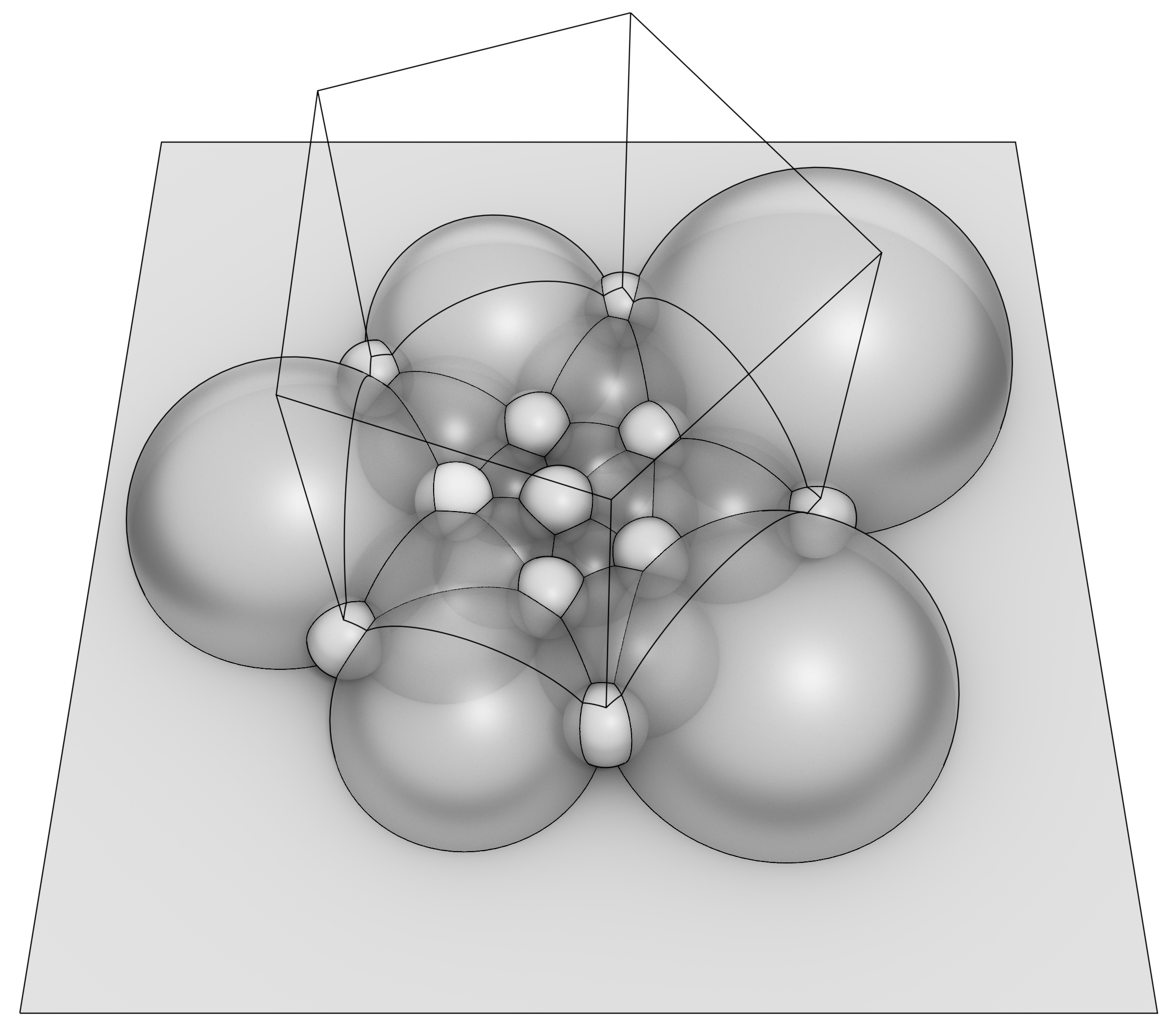
Figure 1: Ideal polyhedron (bounded by the transparent hyperbolic planes) decorated with horospheres (white) at ideal vertices

Assume that one ideal vertex, $v_{\infty}$, is the point at infinity in the half-space model. The faces of $P$ are ideal polygons. Should any face have more than three sides, triangulate it by adding diagonal ideal arcs. The diagonals may be chosen arbitrarily, except in vertical faces incident with $v_{\infty}$, which should be triangulated by adding the vertical diagonals incident with $v_{\infty}$.

For every ideal vertex $v$ of $P$, choose a horosphere $s_{v}$ centered at $v$ as follows: Choose an arbitrary horosphere $s_{v_{\infty}}$ at $v_{\infty}$ (not shown in Figure 1). For all other vertices $v\not=v_{\infty}$ let $s_{v}$ be the horosphere centered at $v$ that touches $s_{v_{\infty}}$ (white spheres in Figure 1). For each edge $e$ not incident with $v_{\infty}$ let $\tilde{\lambda}_{e}$ be the signed distance (see Figure 2) of the horospheres at the ends of $e$.

3pt $\lambda>0$ [b] <0pt,0pt> at 85 42 $\lambda<0$ [b] at 218 21

Figure 2: Signed distance $\lambda$ of disjoint and intersecting horocycles

For each edge $e$ incident with $v_{\infty}$, let $\tilde{\lambda}_{e}=\infty$.

Intrinsically, the ideal polyhedron $P$ is the hyperbolic surface $S$. The triangulated faces of $P$ form an ideal triangulation $\widetilde{\Delta}$ of $S$. The horospheres $s_{v}$ at the vertices of $P$ intersect the surface $S$ in horocycles $h_{v}=s_{v}\cap P$. The signed distance $\tilde{\lambda}_{e}$ of horospheres in $H^{3}$ is also the intrinsic signed distance of the corresponding horocycles in $S$ along the ideal arc $e$. By Proposition 6.2, $(\widetilde{\Delta},\tilde{\lambda})$ are realizable coordinates with distinguished vertex $v_{\infty}$ as defined in Definition 6.1.

To reconstruct the realization $P$ from $(\widetilde{\Delta},\tilde{\lambda})$, proceed as follows: For each triangle $t\in T_{\widetilde{\Delta}}$ that is not incident with $v_{\infty}$, construct an ideal tetrahedron as shown in Figure 3.

2pt $\raisebox{10.0pt}{\Big{\uparrow}}v_{\infty}$ [ ] at 130 270 $v_{1}$ [t] at 69 108 $v_{2}$ [t] at 156 77 $v_{3}$ [t] at 138 164 $\lambda_{3}$ [t] at 110 109 $\ell_{3}$ [b] at 115 118 $\lambda_{1}$ [r] at 150.5 133.5 $\ell_{1}$ [l] <-3pt,7pt> at 154 129 $\lambda_{2}$ [tl] at 101 152 $\ell_{2}$ [br] at 98 159 $\alpha_{1}$ [ ] at 78 135 $\alpha_{2}$ [ ] at 151 112 $\alpha_{3}$ [ ] at 137 181 $A_{1}$ [r] at 66 134 $A_{2}$ [l] at 159 104 $A_{3}$ [l] at 141 193

Figure 3: Ideal tetrahedron decorated with horospheres at the vertices. The horosphere at $v_{\infty}$ is the horizontal plane at height $1$. The horospheres at $v_{1}$, $v_{2}$, $v_{3}$ touch the horosphere at $v_{\infty}$. The horosphere at $v_{\infty}$ intersects the tetrahedron in a euclidean triangle with sides $\ell_{i}=e^{\frac{1}{2}\lambda_{i}}$, where $\lambda_{i}$ are the signed distances between horospheres (see Figure 4).

2pt $\ell=e^{\frac{1}{2}\lambda}$ [b] at 63 45 $\lambda$ [t] at 63 33

Figure 4: Signed distance $\lambda$ and horocyclic arc length $\ell$ in a configuration of two horocycles that are tangent to a third horocycle

These tetrahedra fit together to form the ideal polyhedron $P$. This construction of a realizing polyhedron works for any coordinates that are realizable in the sense of Definition 6.1 (see Proposition 6.3).

The intrinsic Problem 2.3 of finding realizable coordinates turns out to be equivalent to a convex optimization problem (see Theorem 7.18). This leads to a proof of Theorem 1.1 (see Section 9).

3 Penner coordinates

In Sections 3–5, we review known results from Teichmüller theory. The aim is to fix notation, to collect required background material and equations for reference, and to translate the convex hull construction into the language of Delaunay decompositions. For the reader’s convenience, we indicate proofs whenever we see a way to do so by a short comment or a suggestive picture. For a more thorough treatment, we refer to the literature. In this section, we review Penner’s coordinates for the decorated Teichmüller spaces of punctured surfaces [22] [23].

Let $S_{g}$ be the oriented surface of genus $g$, let $V\subseteq S_{g}$ be a finite nonempty subset of $n=|V|$ points and let $S_{g,n}=S_{g}\setminus V$ be the oriented surface of genus $g$ with $n$ punctures. The pair $(S_{g},V)$ is the surface of genus $g$ with $n$ marked points. A triangulation of $(S_{g},V)$ is a triangulation with vertex set $V$. We will denote the set of edges by $E_{\Delta}$ and the set of triangles by $T_{\Delta}$. We write $e_{1}(t)$, $e_{2}(t)$, $e_{3}(t)$ for the edges of a triangle $t$ in cyclic order, $e_{1}(v),\ldots,e_{\deg(v)}(v)$ for the edges emanating from a vertex $v$ in cyclic order, and $v_{1}(e)$, $v_{2}(e)$ for the vertices of an edge $e$ (in arbitrary order).

Penner coordinates $(\Delta,\lambda)$ on the decorated Teichmüller space $\widetilde{\mathcal{T}}_{g,n}$ consist of a triangulation $\Delta$ of $(S_{g},V)$ and a function $\lambda\in\mathbb{R}^{E_{\Delta}}$. The Penner coordinates describe a complete hyperbolic surface with finite area of genus $g$ with $n$ cusps, marked by $S_{g,n}$, and decorated with a horocycle at each cusp, together with an ideal triangulation. The cusps correspond to the vertices $v\in V$ and the ideal triangulation corresponds to a triangulation in the isotopy class of $\Delta$. For simplicity, we will identify cusps with vertices and the ideal triangulation with $\Delta$. The value $\lambda_{e}=\lambda(e)$ for an edge $e\in E_{\Delta}$ is the signed distance (see Figure 2) of the horocycles at its ideal vertices $v_{1}(e)$, $v_{2}(e)$ as measured in a lift to the universal cover $H^{2}$.

For two triangulations $\Delta$, $\widetilde{\Delta}$, we denote the chart transition function by

$$\tau_{\Delta,\widetilde{\Delta}}:\mathbb{R}^{E_{\Delta}}\rightarrow\mathbb{R}^{E_{\widetilde{\Delta}}}.$$ (1)

That is, the Penner coordinates $(\Delta,\lambda)$ and $(\widetilde{\Delta},\tilde{\lambda})$ describe the same surface if and only if $\tilde{\lambda}=\tau_{\Delta,\widetilde{\Delta}}(\lambda)$.

Remark 3.1 (notation warning).

Our $\lambda$s denote hyperbolic lengths, not Penner’s lambda-lengths [23]. The lambda-lengths are $e^{\lambda/2}$, and we denote them by $\ell$ in this paper. In earlier articles [22], the lambda-lengths were defined as $\sqrt{2}\,e^{\lambda/2}$.

The decorated Teichmüller space $\widetilde{\mathcal{T}}_{g,n}$ is a fiber bundle over the ordinary Teichmüller space $\mathcal{T}_{g,n}$. The projection map $\pi:\widetilde{\mathcal{T}}_{g,n}\rightarrow\mathcal{T}_{g,n}$ simply forgets about the decoration. The fibers, whose points correspond to choices of decorating horocycles, are naturally affine spaces. If a decorated surface with Penner coordinates $(\Delta,\lambda)$ is chosen as the origin in its fiber, then there is a natural parametrization of the fiber by $\mathbb{R}^{V}$:

Proposition 3.2 (parametrizing a fiber of $\widetilde{\mathcal{T}}_{g,n}$).

Let $\Lambda^{(\Delta,\lambda)}$ be the function

$$\Lambda^{(\Delta,\lambda)}:\mathbb{R}^{V}\longrightarrow\mathbb{R}^{E_{\Delta}},\qquad u\longmapsto\Lambda^{(\Delta,\lambda)}(u)$$

where the value of $\Lambda^{(\Delta,\lambda)}(u)$ for $e\in E_{\Delta}$ is

$$\Lambda^{(\Delta,\lambda)}_{e}(u)=\lambda_{e}+u_{v_{1}(e)}+u_{v_{2}(e)}.$$ (2)

Then the decorated surfaces in the fiber of the surface with coordinates $(\Delta,\lambda)$ are precisely the surfaces with Penner coordinates $(\Delta,\Lambda^{\Delta,\lambda}(u))$ for some $u\in\mathbb{R}^{V}$, and $u$ is uniquely determined by $(\Delta,\lambda)$ and the decorating horocycles. The horocycle of the decorated surface $(\Delta,\Lambda^{\Delta,\lambda}(u))$ at a vertex $v$ is a distance $u_{v}$ away from the horocycle of $(\Delta,\lambda)$ at $v$, measured in the direction of the cusp.

The following two propositions provide relations between $\lambda$s and the lengths of horocyclic arcs.

Proposition 3.3 (horocyclic arcs in a decorated triangle).

Consider a decorated ideal triangle with signed horocycle distances $\lambda_{1}$, $\lambda_{2}$, $\lambda_{3}$ as shown in Figure 5.

2pt $\lambda_{1}$ [t] at 64 45 $\lambda_{2}$ [bl] at 83 63 $\lambda_{3}$ [br] at 44 63 $\alpha_{1}$ [t] at 65.5 78 $\alpha_{2}$ [bl] at 34 44 $\alpha_{3}$ [br] <-0.5pt, -1.5pt> at 96 44.5 2pt $\lambda_{1}$ [bl] <-0.5pt,-0.5pt> at 88 52 $\lambda_{2}$ [l] at 131 85 $\lambda_{3}$ [r] at 44 85 $\alpha_{1}$ [t] at 90.5 117 $\alpha_{2}$ [bl] <-2pt,-1pt> at 56 52.5 $\alpha_{3}$ [br] <1.5pt, 1.5pt> at 126 44 $0$ [t] at 44 9 $1$ [t] at 131 9 $i$ [br] at 42 92 $1+i$ [bl] at 132 92

Figure 5: Decorated ideal triangle in the Poincaré disk model (left) and in the half-plane model (right)

Each horocycle intersects the triangle in an arc of length $\alpha_{k}$. The signed horocycle distances $\lambda$ determine the horocyclic arc lengths $\alpha$, and vice versa, via the relations

$$\alpha_{i} =e^{\frac{1}{2}(\lambda_{i}-\lambda_{j}-\lambda_{k})},$$ (3)

$$\lambda_{i} =-\log\alpha_{j}-\log\alpha_{k},$$ (4)

where $(i,j,k)$ is a permutation of $(1,2,3)$.

Summing the horocyclic arc lengths around one vertex, one obtains the total horocycle length at a cusp:

Proposition 3.4 (horocycle length at a cusp).

The total length of the horocycle at a cusp $v\in V$ of the decorated hyperbolic surface with Penner coordinates $(\Delta,\lambda)$ is

$$c_{v}(\Delta,\lambda)=\sum_{k=0}^{d-1}e^{\frac{1}{2}\left(\lambda_{\widehat{e}_{i}(v)}-\lambda_{e_{i}(v)}-\lambda_{e_{i+1}(v)}\right)},$$ (5)

where $e_{1}(v),\ldots,e_{d}(v)=e_{0}(v)$ are the edges emanating from $v$ in cyclic order and $\hat{e}_{1}(v),\ldots,\hat{e}_{d}(v)=\hat{e}_{0}(v)$ are the edges opposite $v$ in cyclic order, so that the $i$-th triangle around $v$ looks like this:

Shear coordinates $(\Delta,\sigma)$ on the Teichmüller space $\mathcal{T}_{g,n}$ also consist of a triangulation $\Delta$ of $(S_{g},V)$ and a function $\sigma\in\mathbb{R}^{E_{\Delta}}$. Shear coordinates describe a marked surface together with an ideal triangulation but without decorating horocycles. For each edge $e\in E_{\Delta}$, $\sigma_{e}=\sigma(e)$ is the shear with which the ideal triangles are glued together along $e$ (see Figure 6).

2pt $\lambda_{a}$ [tl] at 72 48 $\lambda_{b}$ [bl] at 71 82 $\lambda_{c}$ [br] at 42 64 $\lambda_{d}$ [tr] at 45 31 $\sigma_{e}$ [l] at 57 55 $\alpha$ [b] at 59.5 26 $\beta$ [b] at 52 23

Figure 6: Penner coordinates and shear coordinates

The shear coordinates of a complete hyperbolic surface sum to zero around every cusp:

$$\sum_{i=1}^{\deg(v)}\sigma_{e_{i}(v)}=0.$$ (6)

Proposition 3.5 (Penner coordinates and shear coordinates).

(i) The shear coordinates $(\Delta,\sigma)$ of a decorated surface with Penner coordinates $(\Delta,\lambda)$ are

$$\sigma_{e}=\frac{1}{2}(\lambda_{a}-\lambda_{b}+\lambda_{c}-\lambda_{d})=\log\beta-\log\alpha,$$ (7)

where $a$, $b$, $c$, $d$ are the edges adjacent to edge $e$, and $\alpha$, $\beta$ are the horocycle arc lengths, as shown in Figure 6.

(ii) Conversely, if $(\Delta,\sigma)$ are the shear coordinates of a complete finite area hyperbolic surface $S$, then one obtains Penner coordinates $(\Delta,\lambda)$ for $S$, decorated with some choice of horocycles, as follows. First, note that the shear coordinates determine the length ratios of adjacent horocycle arcs $\alpha$, $\beta$ as shown in Figure 6 by equation (7). Use the relations (7) to determine compatible arc lengths around each vertex. (The equations (7) are compatible by (6), but under-determined: At each vertex, exactly one arc length may be chosen arbitrarily, and this choice fixes the decorating horocycle.) Then use equations (4) to determine $\lambda$.

The Penner coordinates of a decorated surface with respect to triangulations $\Delta$ and $\Delta^{\prime}$ that differ by a single edge flip are related by Ptolemy’s relation (9):

2pt $a$ [t] at 66 46 $b$ [l] at 107 59 $c$ [bl] at 94 78 $d$ [br] at 45 66 $e$ [br] at 71 60 $f$ [tr] <0pt,4pt> at 89 55 $\alpha_{1}$ [t] at 63 80 $\alpha_{2}$ [tl] at 75.5 84

Figure 7: Ptolemy relation

2pt $\alpha$ [ ] at 42 69 $\alpha^{\prime}$ [ ] at 110 64 $\beta$ [ ] at 69 40 $\beta^{\prime}$ [ ] at 81 41.5 $\gamma$ [ ] at 57.5 86 $\gamma^{\prime}$ [ ] at 70 87.5 $e$ [l] at 69 64 $v_{a}$ [r] at 2 74 $v_{b}$ [t] at 88 4 $v_{a^{\prime}}$ [l] at 126 62 $v_{c}$ [b] at 63 126

Figure 8: Local Delaunay condition

Proposition 3.6 (Ptolemy relation).

Consider a decorated ideal quadrilateral with edges $a$, $b$, $c$, $d$ and diagonals $e$, $f$ as shown in Figure 8. Let $\lambda_{a},\ldots,\lambda_{f}$ be the respective signed horocycle distances. Then $\ell_{a},\ldots,\ell_{f}$ defined by

$$\ell=e^{\frac{1}{2}\lambda}$$ (8)

satisfy Ptolemy’s relation

$$\ell_{e}\ell_{f}=\ell_{a}\ell_{c}+\ell_{b}\ell_{d}.$$ (9)

Proof.

This follows with (3) from

$$e^{\frac{1}{2}(\lambda_{a}-\lambda_{d}-\lambda_{f})}+e^{\frac{1}{2}(\lambda_{b}-\lambda_{c}-\lambda_{f})}=\alpha_{1}+\alpha_{2}=e^{\frac{1}{2}(\lambda_{e}-\lambda_{c}-\lambda_{d})}$$

by multiplying both sides with $e^{\frac{1}{2}(\lambda_{c}+\lambda_{d}+\lambda_{f})}$. ∎

4 Ideal Delaunay triangulations

Epstein and Penner’s convex hull construction [10, 22, 23] is a fundamental tool for the polyhedral realization method presented here. The construction works for cusped hyperbolic manifolds of arbitrary dimension, but some aspects are simpler for surfaces (compare, e.g., the local condition (10) with the generalized tilt formula [27]), and other aspects (like the edge flip algorithm [30]) have no adequate counterpart in higher dimensions. In this section, we will review the relevant results focusing on the two-dimensional case.

In order to apply the convex hull construction to polyhedral realization problems, we need to translate it into the language of Delaunay decompositions. This translation is a straightforward application of the pole-polar relationship of projective geometry and Proposition 4.1 below. In the hyperboloid model of the hyperbolic plane, circles are intersections of the hyperboloid with affine planes. Planes intersecting the hyperboloid correspond, via the pole-polar relationship, to points outside the hyperboloid. Two circles intersect orthogonally if the pole of one circle’s plane lies in the other circle’s plane. The vertices of the Epstein–Penner convex hull correspond to horocycles, while the faces correspond to orthogonally intersecting circles. (It may be necessary to scale the convex hull up to make all faces intersect the hyperboloid.) Convexity translates to the condition that a face-circle intersects all horocycles corresponding to non-incident vertices less than orthogonally. So far, everything is analogous to the standard theory of power diagrams and weighted Delaunay triangulations in euclidean space [3]. Proposition 4.1 allows us to express the Delaunay condition in terms of oriented contact instead of orthogonality. This only works for Delaunay triangulations in hyperbolic space and with horospheres as sites.

Proposition 4.1 (orthogonality and contact).

Let $h_{1},\ldots,h_{n}$ be horocycles with different centers in the hyperbolic plane. Of the following statements, any two labeled with the same letter are equivalent. If $n\geq 3$, statements labeled with different letters are mutually exclusive.

• There is a circle that intersects every horocycle $h_{1},\ldots,h_{n}$ orthogonally.

• There is a circle that touches every horocycle $h_{1},\ldots,h_{n}$ externally.

• There is a horocycle that intersects every horocycle $h_{1},\ldots,h_{n}$ orthogonally.

• There is a horocycle that touches every horocycle $h_{1},\ldots,h_{n}$.

• There is a hypercycle that intersects every horocycle $h_{1},\ldots,h_{n}$ orthogonally.

• There is a hypercycle or geodesic that touches every horocycle $h_{1},\ldots,h_{n}$ on the same side.

(A hypercycle is a complete curve at a constant nonzero distance from a geodesic.)

The following definitions and theorems summarize Epstein and Penner’s results in the language of Delaunay decompositions.

Definition 4.2 (ideal Delaunay decomposition).

Let $S$ be a complete finite area hyperbolic surface with at least one cusp, decorated with a horocycle at each cusp. First, assume that the horocycles are small enough so that they bound disjoint cusp neighborhoods. An ideal cell decomposition $D$ of $S$ is an ideal Delaunay decomposition, if its lift $\hat{D}$ to $H^{2}$ and the lifted horocycles satisfy the global Delaunay condition:

• For every face $\hat{f}$ of $\hat{D}$ there is a circle that touches all lifted horocycles centered at the vertices of $\hat{f}$ externally and does not meet any other lifted horocycles.

If the horocycles are not small enough to bound disjoint cusp neighborhoods, the cell decomposition $D$ is an ideal Delaunay decomposition if condition (gD) holds for smaller horocycles at equal distance to the original horocycles. The distance is arbitrary as long as it is large enough for the new horocycles to bound disjoint cusp neighborhoods.

Theorem 4.3 (existence and uniqueness).

For each decorated complete finite area hyperbolic surface with at least one cusp there exists a unique ideal Delaunay decomposition.

The faces of the ideal Delaunay decomposition are ideal polygons. An ideal Delaunay triangulation is obtained by adding ideal arcs to triangulate the non-triangular faces:

Definition 4.4 (ideal Delaunay triangulation).

An ideal triangulation $\Delta$ of a decorated complete finite area hyperbolic surface is a called an ideal Delaunay triangulation if it is a refinement of the ideal Delaunay decomposition $D$, that is, if $E_{D}\subseteq E_{\Delta}$. An edge $e\in E_{\Delta}$ is an essential edge of the Delaunay triangulation if $e\in E_{D}$. The edges in $E_{\Delta}\setminus E_{D}$ are nonessential.

The decorated Teichmüller spaces $\widetilde{\mathcal{T}}_{g,n}$ decompose into cells consisting of all decorated surfaces with the same ideal Delaunay decomposition:

Definition 4.5 (Penner cell).

For a triangulation $\Delta$ of $(S_{g},V)$, $|V|=n$, let the Penner cell $\mathcal{C}(\Delta)$ be the set of decorated surfaces in $\widetilde{\mathcal{T}}_{g,n}$ for which $\Delta$ is an ideal Delaunay triangulation.

Theorem 4.6 (canonical cell decomposition of $\widetilde{\mathcal{T}}_{g,n}$).

The Penner cells $\mathcal{C}(\Delta)\subseteq\widetilde{\mathcal{T}}_{g,n}$ are the top-dimensional closed cells of a cell decomposition of $\widetilde{\mathcal{T}}_{g,n}$.

Like in the standard euclidean theory, the global Delaunay condition (gD) is equivalent to edge-local conditions:

Theorem 4.7 (local Delaunay conditions).

Let $S$ be a complete finite area hyperbolic surface with at least one cusp, decorated with small enough horocycles so they bound disjoint cusp neighborhoods. An ideal triangulation $\Delta$ is a Delaunay triangulation if and only if for every edge $e$, one and hence all of the equivalent conditions (lD1)–(lD3) are satisfied. Note that the directions left and right relative to $e$ are only defined once an orientation is chosen for $e$, but the truth values of conditions (lD1) and (lD2) are independent of this choice.

1. The circle touching the three horocycles of the triangle to the left of $e$ and the remaining horocycle of the triangle to the right of $e$ are disjoint or externally tangent.

2. The center of the circle touching the three horocycles of the triangle to the left of $e$ is to the left of, or coincides with, the center of the circle touching the horocycles of the triangle to the right of $e$.

3. The total length of the horocyclic arcs incident with $e$ is not greater than the total length of the horocyclic arcs opposite to $e$, as shown in Figure 8:

   $$\alpha+\alpha^{\prime}\leq\beta+\beta^{\prime}+\gamma+\gamma^{\prime}.$$ (10)

Moreover, if $\Delta$ is a Delaunay triangulation, then an edge $e$ is nonessential if and only if tangency holds in (lD1), or equivalently, if the circle centers coincide in condition (lD2), or equivalently, if equality holds in (10).

The global Delaunay condition (gD) obviously implies (lD1), and it is not difficult to see that (lD1) and (lD2) are equivalent. To see that (lD2) and (lD3) are equivalent, note that the oriented length of the thick horocyclic arcs in Figure 8 is $-\alpha-\alpha^{\prime}+\beta+\beta^{\prime}+\gamma+\gamma^{\prime}$. It remains to show that the local conditions imply the global condition (gD); see [22, Theorem 5.1] [23, p. 128].

Theorem 4.8 (Weeks’s flip alogrithm [30]).

An ideal Delaunay triangulation of the decorated surface $(\Delta,\lambda)$ can be found by the flip algorithm: Iteratively flip any edge violating the local condition (10) and update $\lambda$ using Ptolemy’s relation (9) until no such edge remains.

Remarks 4.9.

(i) Issues of numerical instability that plague the euclidean flip algorithm [9, 13] are also relevant in this setting.

(ii) No other algorithm for computing ideal Delaunay triangulations seems to be known.

(iii) Because the diameter of the flip-graph is infinite, the number of flips necessary to arrive at a Delaunay triangulation, depending on an arbitrary initial triangulation, is unbounded. (The only exception is the sphere with three punctures, which admits only three ideal triangulations.)

(iv) To analyze the complexity of a variational algorithm to solve the realization problem 2.1, it would be important to bound the number of steps in the flip algorithm under the condition that the initial triangulation is a Delaunay triangulation for a different choice of horocycles.

(v) Little seems to be known about the following related question, except that the number is finite [1]: How many ideal Delaunay decompositions arise for a fixed hyperbolic surface as the decoration varies over all possible choices of horocycles? A recent result says that the lattice of Delaunay decompositions of a fixed punctured Riemann surface is the face lattice of an associated secondary polyhedron [17].

(vi) Recently, an analogous flip algorithm for surfaces with real projective structure was analyzed by Tillmann and Wong [29].

Definition 4.10.

Let

$$\operatorname{\textit{Del}}:(\Delta,\lambda)\longmapsto(\widetilde{\Delta},\tilde{\lambda})$$

be a function that maps the Penner coordinates $(\Delta,\lambda)$ of a decorated surface to the Penner coordinates $(\widetilde{\Delta},\tilde{\lambda})$ of the same decorated surface with respect to an ideal Delaunay triangulation $\widetilde{\Delta}$.

Such a function $\operatorname{\textit{Del}}$ can be computed using the flip algorithm (see Theorem 4.8). The function $\operatorname{\textit{Del}}$ is not uniquely determined because an ideal Delaunay triangulation is in general not unique. We will use $\operatorname{\textit{Del}}$ in situations in which it makes no difference which ideal Delaunay triangulation is chosen.

We will repeatedly use the following fact, which is Lemma 5.2 in [22].

Lemma 4.11 (ideal Delaunay triangulations and triangle inequalities).

Let $(\Delta,\lambda)$ be Penner coordinates and let $\ell\in\mathbb{R}_{>0}^{E}$ be defined by (8). The local Delaunay conditions (10) imply the triangle inequalities for $\ell$ for every triangle $t\in T_{\Delta}$:

$$\begin{split}-\ell_{e_{1}(t)}+\ell_{e_{2}(t)}+\ell_{e_{3}(t)}&>0\\ \ell_{e_{1}(t)}-\ell_{e_{2}(t)}+\ell_{e_{3}(t)}&>0\\ \ell_{e_{1}(t)}+\ell_{e_{2}(t)}-\ell_{e_{3}(t)}&>0.\end{split}$$ (11)

The following theorem says that ideal Delaunay triangulations of a decorated hyperbolic surface are also euclidean Delaunay triangulations of the corresponding piecewise euclidean surface, and vice versa. This ought to be known, but we do not have a reference. Delaunay triangulations and Voronoi diagrams of piecewise euclidean surfaces were invented and reinvented many times in the context of different applications, for example in [7, 16, 19, 28].

Theorem 4.12 (ideal and euclidean Delaunay triangulations).

Let $(\Delta,\lambda)$ be Penner coordinates, and let $\ell\in\mathbb{R}_{>0}^{E_{\Delta}}$ be defined by (8).

(i) If $\Delta$ is an ideal Delaunay triangulation of the decorated surface described by the Penner coordinates $(\Delta,\lambda)$, then $\ell$ satisfies the triangle inequalities (11) by Lemma 4.11. So we may equip the surface $S_{g}$ with the piecewise euclidean metric that turns each triangle $t\in T_{\Delta}$ into a euclidean triangle and each edge $e\in E_{\Delta}$ into a euclidean line segment of length $\ell_{e}$. Then $\Delta$ is also a Delaunay triangulation of this piecewise euclidean surface.

(ii) Conversely, if $\ell$ satisfies the triangle inequalities for every triangle $t\in T_{\Delta}$, and if $\Delta$ is a Delaunay triangulation for $S_{g}$ equipped with the piecewise euclidean metric described in (i), then $\Delta$ is also an ideal Delaunay triangulation of the decorated hyperbolic surface with Penner coordinates $(\Delta,\lambda)$.

Proof.

First note that a decorated ideal tetrahedron with horosphere distances $\lambda_{i}$ as shown in Figure 3 exists if and only if the $\ell_{i}$ defined by (8) satisfy the triangle inequalities. Now consider two decorated ideal tetrahedra as shown in Figure 3 glued along two matching vertical faces. The local Delaunay condition (lD2) for the decorated ideal triangles in the base planes is equivalent to the local Delaunay condition for the euclidean triangles in which the horocycle at $v_{\infty}$ intersects the tetrahedra. To see this, note that the circumcenters of the euclidean triangles project vertically down to the highest points of the hyperbolic base planes, and that these points are the centers of circles touching the incident horocycles. ∎

5 Akiyoshi’s compactification

Every triangulation $\Delta$ of $(S_{g},V)$ with $n=|V|>0$, $2-2g-n<0$ is the Delaunay decomposition for some decorated complete finite area hyperbolic metric on $S_{g,n}$. For example, the decorated surface $(\Delta,\lambda)$ with Penner coordinates $\lambda=0$ has Delaunay decomposition $\Delta$. There are infinitely many triangulations of $(S_{g},V)$, unless $g=0$ and $n\leq 3$. However, a fixed hyperbolic surface supports only a finite number of ideal Delaunay triangulations:

Theorem 5.1 (Akiyoshi [1]).

Let $S$ be a complete hyperbolic surface of finite area with at least one cusp. There are only finitely many ideal triangulations $\Delta$ of $S$ such that there exists a decoration of $S$ with horocycles such that $\Delta$ is a Delaunay triangulation of the decorated surface.

In fact, Akiyoshi proved a more general result, the generalization of Theorem 5.1 to hyperbolic manifolds of arbitrary dimension. A simpler proof for the two-dimensional case can be found in [15].

Akiyoshi’s proof is based on the observation that the convex hull construction of Epstein and Penner generalizes naturally to partially decorated surfaces, that is, complete hyperbolic surfaces of finite area, decorated with horocycles at some, but at least one, of the cusps. A missing horocycle should be interpreted as the limit of horocycles vanishing at infinity. The existence and uniqueness Theorem 4.3 generalizes to partially decorated surfaces:

Theorem 5.2 (existence and uniqueness).

Every partially decorated surface has a unique ideal Delaunay decomposition.

However, Definition 4.2 of an ideal Delaunay decompositions has to be modified quite radically: an ideal Delaunay decomposition of a partially decorated surface with missing horocycles is not an ideal cell decomposition (see Definition 5.4). A cusps with missing horocycle is contained in a Delaunay face that is not an ideal polygon, but an ideal polygon with a cusp in the sense of the following definition:

Definition 5.3.

An ideal polygon with a cusp is a hyperbolic manifold-with-boundary $f$ of finite area whose interior is homeomorphic to an open disk with one puncture such that a neighborhood of the puncture corresponds to a cusp neighborhood in $f$ and the boundary is a union of complete geodesics (see Figure 9).

Figure 9: An ideal polygon with a cusp (shaded region), which is a face of a Delaunay decomposition of a partially decorated surface. The left and right boundary are identified by an isometry $z\mapsto z+c$. The vertical edges are nonessential edges of an adjusted Delaunay triangulation.

However, the Delaunay decomposition of a partially decorated surface is a cell decomposition when viewed as a decomposition of $(S_{g},V)$, the closed surface of genus $g$ with marked points. The faces are cells, but the marked points $v\in V$ that correspond to cusps without decorating horocycle are not vertices of the decomposition. A face contains at most one marked point in its interior, which we call the central vertex of the face (although it is not a vertex of the decomposition). Let us call the regular vertices of an ideal polygon with a cusp its peripheral vertices to distinguish them from its central vertex.

Definition 5.4 (Delaunay decomposition of a partially decorated surface).

Let $D$ be a decomposition of a partially decorated surface into ideal polygons and ideal polygons with a cusp, called the faces of the decomposition. Suppose first that the decorating horocycles are disjoint. Then the decomposition $D$ is called a Delaunay decomposition, if its lift $\hat{D}$ to $H^{2}$ and the lifted horocycles satisfy the following conditions:

• If $\hat{f}$ is the lift of a face of $D$ that is an ideal polygon, then there is a circle that touches all lifted horocycles at the vertices of $\hat{f}$ externally and does not meet any other lifted horocycles.

• If $\hat{f}$ is the lift of a face $f$ of $D$ that is an ideal polygon with a cusp, then every peripheral vertex of $f$ is decorated with a horocycle, and there exists a horocycle centered at the lifted central vertex of $\hat{f}$ that touches the lifted horocycles at the lifted peripheral vertices of $\hat{f}$ and does not meed any other lifted horocycles.

Extend this Definition to the case of intersecting horocycles like in Definition 4.2.

Remark 5.5.

Generically, the punctured Delaunay faces are punctured monogons. Such punctured monogons were already considered by Penner to construct coordinates on the Teichmüller space of partially decorated punctured surfaces [22, Addendum] [23, Sec. 5.1].

Even if a cusp is not decorated with a horocycle, differences of distances to horocycles at other cusps are well defined. This can be used to characterize the punctured Delaunay faces (see Figure 9):

Proposition 5.6 (characterization of punctured Delaunay faces).

Let $S$ be a partially decorated surface, let $v$ be a cusp with missing horocycle, and let $p$ be an ideal polygon with a cusp in $S$ whose central vertex is $v$. Then $p$ is a face of the Delaunay decomposition of $S$ if and only if all peripheral vertices of $p$ are decorated with horocycles, and these horocycles have all the same distance to $v$, and this distance is strictly smaller than the distance of any other horocycle to $v$.

Definition 4.4 of ideal Delaunay triangulations and essential and nonessential edges remains valid without change. However, it will be useful to triangulate the punctured Delaunay faces in a canonical way:

Definition 5.7 (adjusted Delaunay triangulation).

An ideal triangulation $\Delta$ of a partially decorated surface is called an adjusted Delaunay triangulation if it refines the ideal Delaunay decomposition and every punctured face is triangulated by adding the ideal arcs connecting the central vertex with the peripheral vertices.

Theorem 4.7 on local Delaunay conditions remains valid after the following modifications: A triangle of a Delaunay triangulation has at most one vertex with missing horocycle. For an ideal triangle with missing horocycle at one vertex $v$, one has to consider the horocycle centered at $v$ and touching the triangle’s two horocycles, instead of a circle touching three horocycles. If a horocycle is missing, the respective arc length in condition (10) is zero.

The flip algorithm (see Theorem 4.8) remains valid, but some details have to be modified (see Proposition 5.9) because Penner coordinates $(\Delta,\lambda)$ do not describe partially decorated surfaces. Instead, we may use the parametrization of a fiber of $\widetilde{\mathcal{T}}_{g,n}$ described in Proposition 3.2, which extends nicely to partially decorated surfaces:

Definition 5.8 (parametrizing an extended fiber of $\widetilde{\mathcal{T}}_{g,n}$).

Let $(\Delta,\lambda)$ be Penner coordinates for a decorated surface in $\widetilde{\mathcal{T}}_{g,n}$, let

$$\overline{\mathbb{R}}=\mathbb{R}\cup\{+\infty\},$$ (12)

and

$$u\in\overline{\mathbb{R}}^{V}\setminus\{+\infty_{V}\},$$

where $+\infty_{V}$ denotes the constant function $+\infty$ on $V$. Let the partially decorated surface $(\Delta,\lambda,u)$ be the surface obtained from the decorated surface $(\Delta,\lambda)$ by moving, for each vertex $v$, the horocycle at $v$ a distance $u(v)$ in the direction of the cusp $v$. If $u(v)=+\infty$, the horocycle at $v$ is missing. In particular, for $u\in\mathbb{R}^{V}$, the surface $(\Delta,\lambda,u)$ is just the decorated surface with Penner coordinates $(\Delta,\Lambda^{\Delta,\lambda}(u))$.

If (10) is the local Delaunay condition at edge $e\in E_{\Delta}$ for the decorated surface $(\Delta,\lambda)$, then the local Delaunay condition at $e$ for the partially decorated surface $(\Delta,\lambda,u)$ is

$$\alpha e^{-u(v_{a})}+\alpha^{\prime}e^{-u(v_{a^{\prime}})}\leq(\beta+\beta^{\prime})e^{-u(v_{b})}+(\gamma+\gamma^{\prime})e^{-u(v_{c})},$$ (13)

where $e^{-\infty}=0$.

Proposition 5.9 (flip algorithm for partially decorated surfaces).

An ideal Delaunay triangulation of the partially decorated surface $(\Delta,\lambda,u)$ can be found by Weeks’s flip algorithm (see Theorem 4.8) with the local condition (10) replaced by (13). An adjusted Delaunay triangulation can then be found by iteratively flipping all nonessential edges opposite an undecorated cusp until no such edge remains.

With Proposition 5.10 below, the correctness of this algorithm for partially decorated surfaces can be deduced from the correctness of the original algorithm for decorated surfaces.

Proposition 5.10.

If $\widetilde{\Delta}$ is an adjusted Delaunay triangulation for the partially decorated surface $(\Delta,\lambda,u)$, then there is an $M\in\mathbb{R}$ such that $\widetilde{\Delta}$ is also an ideal Delaunay triangulation for the decorated surfaces $(\Delta,\Lambda^{\Delta,\lambda}(\tilde{u}))$ with $\tilde{u}\in\mathbb{R}^{V}$ satisfying

$$\tilde{u}(v) =u(v)\quad \text{if}\quad u(v)<+\infty,$$

$$\tilde{u}(v) >M\quad \text{if}\quad u(v)=+\infty.$$

This is a corollary of the characterization of punctured Delaunay faces in terms of horocycle distances (see Proposition 5.6).

Definition 5.11 (generalized Penner coordinates).

If $\Delta$ is an arbitrary triangulation of a partially decorated surface, then the surface is in general not determined by $\Delta$ and the function $\lambda\in\overline{\mathbb{R}}^{E}$ of horocycle distances, which takes the value $+\infty$ if the horocycle at one or both ends is missing. However, if $\Delta$ is an adjusted Delaunay triangulation, then the pair $(\Delta,\lambda)$ determines the partially decorated surface uniquely (see Proposition 5.6), and we call such a pair generalized Penner coordinates.

Definition 5.12.

Let $\operatorname{\textit{Del}}$ also denote a function

$$\operatorname{\textit{Del}}:(\Delta,\lambda,u)\longmapsto(\widetilde{\Delta},\tilde{\lambda})$$

that maps the parameters $(\Delta,\lambda,u)$ of a partially decorated surface to generalized Penner coordinates $(\widetilde{\Delta},\tilde{\lambda})$ of the same partially decorated surface, where $\widetilde{\Delta}$ is an adjusted Delaunay triangulation. Hence

$$\tilde{\lambda}=\Lambda^{\widetilde{\Delta},\tau_{\Delta,\widetilde{\Delta}}(\lambda)}(u)\,\in\overline{\mathbb{R}}^{E_{\widetilde{\Delta}}},$$

where $\tau_{\Delta,\widetilde{\Delta}}:\mathbb{R}^{E_{\Delta}}\rightarrow\mathbb{R}^{E_{\widetilde{\Delta}}}$ is the chart transition function mapping Penner coordinates with respect to $\Delta$ to Penner coordinates with respect to $\widetilde{\Delta}$.

Such a function $\operatorname{\textit{Del}}$ can be computed by the modified flip algorithm of Proposition 5.9.

The bounds constraints in the variational principle of Theorem 7.18 involve signed distances of horocycles in a decorated surface, which are defined as follows:

Definition 5.13 (signed distance of horocycles).

Let $\delta_{\Delta,\lambda}(v_{1},v_{2})$ denote the signed distance of the horocycles at the vertices $v_{1},v_{2}\in V$ in the decorated surface with Penner coordinates $(\Delta,\lambda)$. More precisely, let

$$\delta_{\Delta,\lambda}(v_{1},v_{2})=\min_{h_{1},h_{2}}d(h_{1},h_{2})$$ (14)

where $d$ denotes the signed distance of horocycles in $H^{2}$ and the minimum is taken over all pairs of horocycles $h_{1}\not=h_{2}$ in $H^{2}$ that are lifts of the horocycles at $v_{1}$ and $v_{2}$, respectively.

Remark 5.14.

The distance $\delta_{\Delta,\lambda}(v_{1},v_{2})$ is well defined and non-trivial even for $v_{1}=v_{2}$, but we will not need this.

Proposition 5.6 implies that the horocycle distances $\delta_{\Delta,\lambda}$ can be calculated using the flip algorithm:

Proposition 5.15 (Calculating $\delta_{\Delta,\lambda}$).

Let $(\Delta,\lambda)$ be Penner coordinates for a decorated surface, let $v_{1},v_{2}\in V$, let

$$u\in\overline{\mathbb{R}}^{V},\qquad u(v)=\begin{cases}0&\text{if }v=v_{2}\\ +\infty&\text{otherwise},\end{cases}$$

and let $(\widetilde{\Delta},\tilde{\lambda},u)$ be the output of the modified flip algorithm (see Proposition 5.9). Then $v_{1}$ is the central vertex of a punctured face of $\widetilde{\Delta}$ and all peripheral vertices are $v_{2}$. For any edge $e\in E_{\widetilde{\Delta}}$ connecting $v_{1}$ and $v_{2}$

$$\delta_{\Delta,\lambda}(v_{1},v_{2})=\tilde{\lambda}_{e}.$$

6 Realizable coordinates

In this section, we characterize the Penner coordinates that may be obtained from an ideal polyhedron by the construction described in Section 2: They are realizable coordinates by Definition 6.1 (see Proposition 6.2). Conversely, for given realizable coordinates, a corresponding ideal polyhedron is uniquely determined by an explicit construction (see Proposition 6.3).

Definition 6.1 (realizable coordinates).

Let $S$ be a complete finite area hyperbolic surface of genus $0$ with $n\geq 3$ cusps. Realizable coordinates for $S$ with distinguished vertex $v_{\infty}\in V$ are a pair $(\widetilde{\Delta},\tilde{\lambda})$ consisting of a triangulation $\widetilde{\Delta}$ of $(S_{0},V)$ and an function $\tilde{\lambda}=\overline{\mathbb{R}}^{E_{\widetilde{\Delta}}}$, where $\overline{\mathbb{R}}=\mathbb{R}\cup\{+\infty\}$, satisfying the following conditions (r1) and (r2):

1. $\widetilde{\Delta}$ is an adjusted Delaunay triangulation for a decoration of $S$ with exactly one missing horocycle at $v_{\infty}$, and $(\widetilde{\Delta},\tilde{\lambda})$ are the corresponding generalized Penner coordinates (see Definition 5.11).

2. Let $\widetilde{\Delta}^{\circ}$ be the subcomplex of $\widetilde{\Delta}$ consisting of all closed cells not incident with $v_{\infty}$, i.e.,

   $$V_{\widetilde{\Delta}^{\circ}} =V\setminus\{v_{\infty}\},$$ (15)

   $$E_{\widetilde{\Delta}^{\circ}} =\{e\in E_{\widetilde{\Delta}}\;|\;e\text{ not incident with }v_{\infty}\},$$ (16)

   $$T_{\widetilde{\Delta}^{\circ}} =\{t\in T_{\widetilde{\Delta}}\;|\;t\text{ not incident with }v_{\infty}\}.$$ (17)

   Then either (r2a) or (r2b) are true:

   • $T_{\widetilde{\Delta}^{\circ}}=\emptyset$, and $\widetilde{\Delta}^{\circ}$ is a linear graph, that is, a graph of the form

     $$\bullet-\bullet-\cdots-\bullet.$$

   • $T_{\widetilde{\Delta}^{\circ}}\not=\emptyset$ and $\widetilde{\Delta}^{\circ}$ is a triangulation of a closed disk. Moreover,

     $$\widetilde{\Theta}_{v} =2\pi\quad v \widetilde{\Delta}^{\circ}$$ if is an interior vertex of , (18)

     $$\widetilde{\Theta}_{v} \leq\pi\quad v \widetilde{\Delta}^{\circ}$$ if is a boundary vertex of , (19)

     where

     $$\widetilde{\Theta}_{v}=\text{ sum of angles around $v$ in $\widetilde{\Delta}^{\circ}{}$},$$ (20)

     measured in the piecewise euclidean metric that that turns each triangle in $T_{\widetilde{\Delta}^{\circ}}$ into a euclidean triangle and each edge in $e\in E_{\widetilde{\Delta}^{\circ}}$ into a euclidean line segment of length $\tilde{\ell}_{e}$, where

     $$\tilde{\ell}=e^{\frac{1}{2}\tilde{\lambda}}.$$ (21)

Proposition 6.2 (ideal polyhedron $\rightarrow$ realizable coordinates).

Let $P$ be a three-dimensional convex ideal polyhedron or a two-sided ideal polygon in $H^{3}$ realizing a surface $S\in\mathcal{T}_{0,n}$, which has Penner coordinates $(\Delta,\lambda)$ for some decoration. Let $v_{\infty}$ be an ideal vertex of $P$. Let $\widetilde{\Delta}$ be a triangulation obtained by adding diagonals to triangulate all non-triangular faces of $P$. The choice of diagonals is arbitrary except for non-triangular faces incident with $v_{\infty}$, in which the diagonals incident with $v_{\infty}$ are be chosen. Let $s_{\infty}$ be a horosphere centered at $v_{\infty}$. For any other vertex $v$, let $s_{v}$ be the horosphere centered at $v$ and touching $s_{\infty}$. For each edge $e\in E_{\Delta}$ not incident with $v_{\infty}$, let $\tilde{\lambda}_{e}$ be the signed distance of the horospheres at the ends of $e$. If $e$ is incident with $v_{\infty}$, let $\tilde{\lambda}_{e}=\infty$.

Then $(\widetilde{\Delta},\tilde{\lambda})$ are realizable coordinates for $S$.

Proof.

In the case of a two-sided polygon, the statement follows easily from the characterization of punctured Delaunay faces, Proposition 5.6. It remains to consider the case of $P$ being a three-dimensional polyhedron.

To show (r1), first note that for an edge $e$ not incident with $v_{\infty}$, $\lambda_{e}$ is also the intrinsic signed distance of the horocycles $h_{v}=s_{v}\cap P$ at the vertices of $e$. It remains to show that $\widetilde{\Delta}$ is an adjusted Delaunay triangulation. First, the union of triangles incident with $v_{\infty}$ is the Delaunay face around the vertex $v_{\infty}$ with vanished horocycle. Indeed, the horocycle $h_{\infty}$ touches the horocycles at adjacent vertices and does not meet the horocycles at all other vertices.

It remains to show that the local Delaunay conditions (see Theorem 4.7) are satisfied for all edges between two triangles that are not incident with $v_{\infty}$. We may assume without loss of generality that the horosphere $s_{\infty}$ was chosen large enough so that the horospheres at the other vertices are pairwise disjoint. Consider a face $f$ of $P$ that is not incident with $v_{\infty}$. The point in the hyperbolic plane of $f$ that is closest to $s_{\infty}$ is the center of the circle in this plane that touches all horospheres at the vertices of $f$ externally. (See Figure 1: The points closest to $s_{\infty}$ are the highest points in the hemispheres.) Using this fact, it is not difficult to see that the local convexity of the edge $e$ in $P$ is equivalent to the local Delaunay condition (lD2) of Theorem 4.7.

(r2) Since we assume that $P$ is a three-dimensional polyhedron, $\widetilde{\Delta}^{\circ}$ is a triangulation of a closed disk. Now (r2b) follows by decomposing $P$ into ideal tetrahedra as shown in Figure 3, one tetrahedron for each triangle in $\widetilde{\Delta}^{\circ}$. The horosphere $s_{\infty}$ intersects these tetrahedra in euclidean triangles with side lengths $\tilde{\ell}$ determined by (21). This implies (18) and (19) because $P$ intersects $s_{\infty}$ in a convex euclidean polygon. ∎

Proposition 6.3 (realizable coordinates $\rightarrow$ ideal polyhedron).

Let $(\widetilde{\Delta},\tilde{\lambda})$ be realizable coordinates of a surface $S\in\mathcal{T}_{0,n}$. Let $\widetilde{\Delta}^{\circ}$ be the subcomplex of $\widetilde{\Delta}$ defined in Definition 6.1 (r2).

(i) If $\widetilde{\Delta}^{\circ}$ is a triangulation of a closed disk, one obtains a polyhedral realization of $S$ as follows: Construct a decorated ideal tetrahedron as shown in Figure 3 for each triangle of $\widetilde{\Delta}^{\circ}$. These ideal tetrahedra fit together to form a polyhedron that realizes $S$.

(ii) If $\widetilde{\Delta}^{\circ}$ is a linear graph then $\widetilde{\Delta}$ is a decomposition of $S$ into partially decorated ideal triangles that fit together to form a realization of $S$ as two-sided ideal polygon.

We omit a detailed proof. The tetrahedra in (i) exist by Lemma 4.11. They fit together to form an ideal polyhedron realizing $S$ by (r2b). That the polyhedron is convex follows from inequality (19) and from the fact that $\widetilde{\Delta}$ is a Delaunay triangulation.

The realizable coordinates $(\widetilde{\Delta},\tilde{\lambda})$ with distinguished vertex $v_{\infty}$ that are obtained from a polyhedron or two-sided polygon by Proposition 6.2 are not uniquely determined:

• Non-triangular faces that are not incident with $v_{\infty}$ may be triangulated in different ways.

• A different choice of horosphere $s_{\infty}$ leads to realizable coordinates $(\widetilde{\Delta},\tilde{\lambda}+h\mathbf{1}_{E_{\widetilde{\Delta}}})$ for some $h\in\mathbb{R}$.

But these are the only sources of ambiguity: If $(\widetilde{\Delta},\tilde{\lambda})$ and $(\widetilde{\Delta}^{\prime},\tilde{\lambda}^{\prime})$ are both realizable coordinates obtained from the same polyhedron or two-sided polygon with the same distinguished vertex $v_{\infty}$ by Proposition 6.2, then

• $\widetilde{\Delta}$ and $\widetilde{\Delta}^{\prime}$ are both adjusted Delaunay triangulations of the same ideal Delaunay decomposition,

• $\tilde{\lambda}^{\prime}=\tau_{\widetilde{\Delta},\widetilde{\Delta}^{\prime}}(\tilde{\lambda}+h\mathbf{1}_{E_{\widetilde{\Delta}}})$ for some $h\in\mathbb{R}$.

Conversely, the polyhedra obtained from different realizable coordinates $(\widetilde{\Delta},\tilde{\lambda})$ and $(\widetilde{\Delta}^{\prime},\tilde{\lambda}^{\prime})$ with the same distinguished vertex $v_{\infty}$ are congruent (as polyhedra marked by $(S_{0},V)$) if and only if conditions (u1) and (u2) are satisfied.

Definition 6.4 (equivalent realizable coordinates).

Realizable coordinates $(\widetilde{\Delta},\tilde{\lambda})$ and $(\widetilde{\Delta}^{\prime},\tilde{\lambda}^{\prime})$ with distinguished vertex $v_{\infty}$ are equivalent if they satisfy conditions (u1) and (u2).

Realizable coordinates are equivalent if and only if they correspond to congruent realizations.

7 The variational principle

In this section we present a variational principle (see Theorem 7.18) for Problem 2.3 of finding realizable coordinates. The variational principle involves the function $\bar{\mathcal{E}}^{v_{\infty}}_{\Delta,\lambda}(u)$ (see Definition 7.16). The variables $u\in\mathbb{R}^{V\setminus\{v_{\infty}\}}$ parametrize a part of the extended fiber of $\widetilde{\mathcal{T}}_{g,n}$ over the surface $(\Delta,\lambda)$. More precisely, they parametrize the horocycle decorations of that surface with missing horocycle at $v_{\infty}$. The variables are subject to bounds constraints, which ensure that the horocycles do not intersect an arbitrary but fixed horocycle at $v_{\infty}$. The definition of $\bar{\mathcal{E}}^{v_{\infty}}_{\Delta,\lambda}(u)$ requires some preparation. After the following brief summary, a detailed account begins with Definition 7.1.

The function $f(x_{1},x_{2},x_{3})$ (see Definition 7.1) provides a variational encoding of euclidean trigonometry: If the variables $x_{i}$ are the logarithmic side lengths of a euclidean triangle, then the partial derivatives of $f$ are its angles (see Proposition 7.2).

Using this building block, the function $\lambda\mapsto\scalebox{0.94}{$\mathsf{H}$}_{\Theta}(\Delta,\lambda)$ (see Definition 7.3) is defined on an open subset $A_{\Delta}$ of the decorated Teichmüller space $\widetilde{\mathcal{T}}_{g,n}$. The function $\scalebox{0.94}{$\mathsf{E}$}_{\Theta,\Delta,\lambda}(u)$ (see Definition 7.5) is the restriction of $\scalebox{0.94}{$\mathsf{H}$}_{\Theta}(\Delta,\,\cdot\,)$ to the intersection of $A_{\Delta}$ with the fiber of $\widetilde{\mathcal{T}}_{g,n}$ over the surface $(\Delta,\lambda)$. This function was already used in a previous article (see Remark 7.6).

Next we extend the function $\scalebox{0.94}{$\mathsf{H}$}_{\Theta}(\Delta,\lambda)$ to the whole decorated Teichmüller space and the function $\scalebox{0.94}{$\mathsf{E}$}_{\Theta,\Delta,\lambda}(u)$ to a whole fiber by adapting the triangulation appropriately. To this end, consider the restriction of $\scalebox{0.94}{$\mathsf{H}$}_{\Theta}(\Delta,\,\cdot\,)$ to the closed Penner cell of all $\lambda\in\mathbb{R}^{E_{\Delta}}$ for which $\Delta$ is a Delaunay triangulation of the decorated surface $(\Delta,\lambda)$. For different triangulations $\Delta$, these restrictions of $\scalebox{0.94}{$\mathsf{H}$}_{\Theta}(\Delta,\,\cdot\,)$ fit together to define a $C^{2}$ function $\mathcal{H}_{\Theta}$ on the whole decorated Teichmüller space $\widetilde{\mathcal{T}}_{g,n}$ (see Corollary 7.10). We denote by $\mathcal{H}_{\Theta,\Delta}(\lambda)$ the representation of $\mathcal{H}_{\Theta}$ in the global Penner coordinate system belonging to the ideal triangulation $\Delta$ (see Definition and Proposition 7.9). The convex function $\mathcal{E}_{\Theta,\Delta,\lambda}(u)$ (see Definition 7.11) is the restriction of $\mathcal{H}_{\Theta,\Delta}(\lambda)$ to the fiber of $\widetilde{\mathcal{T}}_{g,n}$ over $(\Delta,\lambda)$. Finally, $\bar{\mathcal{E}}^{v_{\infty}}_{\Delta,\lambda}(u)$ is obtained by setting $\Theta_{v_{\infty}}=0$ and $\Theta_{v}=2\pi$ for $v\not=v_{\infty}$, and taking the limit $u_{v_{\infty}}\rightarrow+\infty$ (see Definition 7.16).

2pt $x_{1}$ [l] at 241 120 $x_{2}$ [b] at 120 240 $\mathcal{A}$ [ ] at 137 142

Figure 10: Intersection of the domain $\mathcal{A}$ with the plane $x_{3}=0$. The domain $\mathcal{A}$ is invariant with respect to translations in the scaling direction $(1,1,1)$.

Definition 7.1 (the triangle function $f$).

Let $f$ be the function

$$f:\mathbb{R}^{3}\supseteq\mathcal{A}\longrightarrow\mathbb{R},$$

$$f(x_{1},x_{2},x_{3})=\alpha_{1}x_{1}+\alpha_{2}x_{2}+\alpha_{3}x_{3}+\mbox{L}(\alpha_{1})+\mbox{L}(\alpha_{2})+\mbox{L}(\alpha_{3}),$$ (22)

where

$$\mathcal{A}=\left\{\begin{pmatrix}x_{1}\\ x_{2}\\ x_{3}\end{pmatrix}\in\mathbb{R}^{3}\ \middle|\ \begin{aligned} e^{x_{1}}&>e^{x_{2}}+e^{x_{3}},\\ e^{x_{2}}&>e^{x_{3}}+e^{x_{1}},\\ e^{x_{3}}&>e^{x_{1}}+e^{x_{2}}\end{aligned}\right\}$$

(see Figure 10), L is Milnor’s Lobachevsky function [20],

$$\mbox{L}(\alpha)=-\int_{0}^{\alpha}\log\big{|}2\sin(t)\big{|}\,dt$$ (23)

(see Figure 12), and $\alpha_{j}$ are the angles in a triangle with sides $e^{x_{j}}$ as shown in Figure 12.

2pt $\alpha$ [ ] at 280 81.5 $y$ [ ] at 28 168 $y=\mbox{L}(\alpha)$ [ ] at 130 150

2pt $e^{x_{1}}$ [bl] at 61 35 $e^{x_{2}}$ [br] <1pt,-1pt> at 23 31 $e^{x_{3}}$ [t] at 44 5 $\alpha_{1}$ [ ] at 13 7 $\alpha_{2}$ [ ] at 71 14.5 $\alpha_{3}$ [ ] at 43 45

Figure 11: Milnor’s Lobachevsky function L is $\pi$-periodic, odd, and analytic except at $\alpha\in\pi\,\mathbb{Z}$, where the derivative tends to $+\infty$.

Figure 12: Triangle with sides $e^{x_{1}}$, $e^{x_{2}}$, $e^{x_{3}}$

Proposition 7.2 (properties of $f$).

(i) The function $f$ is analytic, and it satisfies the scaling relation

$$f(x_{1}+h,x_{2}+h,x_{3}+h)=\pi h.$$ (24)

(ii) The partial derivatives of $f$ are

$$\frac{\partial f}{\partial x_{i}}=\alpha_{i}.$$ (25)

(iii) The second derivative of $f$ is

$$D^{2}f|_{x}=\cot\alpha_{1}(dx_{2}-dx_{3})^{2}+\cot\alpha_{2}(dx_{3}-dx_{1})^{2}+\cot\alpha_{3}(dx_{1}-dx_{2})^{2}$$ (26)

(iv) The second derivative $D^{2}f|_{x}$ is positive semidefinite with one-dimensional kernel spanned by $(1,1,1)$. In particular, $f$ is locally convex.

See [5, Sec. 4.2] for proofs.

Definition 7.3 (the function $\scalebox{0.94}{$\mathsf{H}$}_{\Theta}$).

For a triangulation $\Delta$ of $(S_{g},V)$ and $\Theta\in\mathbb{R}^{V}$, let

$$\scalebox{0.94}{$\mathsf{H}$}_{\Theta}(\Delta,\,\cdot\,):A_{\Delta}\longrightarrow\mathbb{R},$$

$$\begin{split}\scalebox{0.94}{$\mathsf{H}$}_{\Theta}{}(\Delta,\lambda)=\sum_{t\in T_{\Delta}}2f\Big{(}\frac{\lambda_{e_{1}(t)}}{2},\frac{\lambda_{e_{2}(t)}}{2},\frac{\lambda_{e_{3}(t)}}{2}\Big{)}&-\pi\sum_{e\in E_{\Delta}}\lambda_{e}\\ &-\sum_{v\in V}\Theta_{v}\log c_{v}(\Delta,\lambda),\end{split}$$ (27)

where $A_{\Delta}\subseteq\mathbb{R}^{E_{\Delta}}$ is the subset

$$A_{\Delta}=\big{\{}\lambda\in\mathbb{R}^{E_{\Delta}}\;\big{|}\;\tfrac{1}{2}\big{(}\lambda_{e_{1}(t)},\lambda_{e_{2}(t)},\lambda_{e_{3}(t)}\big{)}\in\mathcal{A}\text{ for all }t\in T_{\Delta}\big{\}},$$ (28)

and $c_{v}$ is defined by (5).

Proposition 7.4 (properties of $\scalebox{0.94}{$\mathsf{H}$}_{\Theta}$).

(i) The function $\scalebox{0.94}{$\mathsf{H}$}_{\Theta}(\Delta,\,\cdot\,)$ is analytic and satisfies the scaling relation

$$\scalebox{0.94}{$\mathsf{H}$}_{\Theta}(\Delta,\lambda+h\,\mathbf{1}_{E_{\Delta}})=\scalebox{0.94}{$\mathsf{H}$}_{\Theta}(\Delta,\lambda)+h\,\pi\Big{(}|T_{\Delta}|-|E_{\Delta}|+\frac{1}{2\pi}\sum_{v\in V}\Theta_{v}\Big{)}.$$ (29)

(ii) For $\Theta=0$, the function $\scalebox{0.94}{$\mathsf{H}$}_{0}(\Delta,\,\cdot\,)$ is convex, and the kernel of the positive semi-definite second derivative is one-dimensional and spanned by $\mathbf{1}_{E_{\Delta}}$.

This follows immediately from the corresponding properties of $f$ and the scaling behavior of $c_{v}$:

$$c_{v}(\Delta,\lambda+h\,\mathbf{1}_{E_{\Delta}})=c_{v}(\Delta,\lambda)-\tfrac{1}{2}h.$$ (30)

Definition 7.5 (the function $\scalebox{0.94}{$\mathsf{E}$}_{\Theta,\Delta,\lambda}$).

Let $\scalebox{0.94}{$\mathsf{E}$}_{\Theta,\Delta,\lambda}$ be the restriction of $\scalebox{0.94}{$\mathsf{H}$}_{\Theta}$ to the fiber of $\widetilde{\mathcal{T}}_{g,n}$ over $(\Delta,\lambda)$ parametrized by $\Lambda^{\Delta,\lambda}$ as defined by (2), that is,

$$\scalebox{0.94}{$\mathsf{E}$}_{\Theta,\Delta,\lambda}:\{u\in\mathbb{R}^{V}\,|\,\Lambda^{\Delta,\lambda}(u)\in A_{\Delta}\}\longrightarrow\mathbb{R}$$

$$\scalebox{0.94}{$\mathsf{E}$}_{\Theta,\Delta,\lambda}(u)=H(\Delta,\Lambda^{\Delta,\lambda}(u)).$$ (31)

Remark 7.6.

The function $\scalebox{0.94}{$\mathsf{E}$}_{\Theta,\Delta,\lambda}(u)$ is up to an additive constant equal to the function $E_{\mathsf{T},\Theta,\lambda}(u)$ (with $\mathsf{T}=\Delta$) defined in the previous article [5, eq. (4-6)]. In that article, the domain of $E_{\mathsf{T},\Theta,\lambda}(u)$ is extended to the whole $\mathbb{R}^{V}$ by exploiting the fact that the function $f$ can be extended to a convex function on the whole $\mathbb{R}^{3}$. Here, we do not need this extension. Instead, we will extend the functions $\scalebox{0.94}{$\mathsf{H}$}_{\Theta}(\Delta,\,\cdot\,)$ and hence also $\scalebox{0.94}{$\mathsf{E}$}_{\Theta,\Delta,\lambda}(u)$ by changing the triangulation (see Definition and Proposition 7.9 and Definition 7.11).

Proposition 7.7 (properties of $\scalebox{0.94}{$\mathsf{E}$}_{\Theta,\Delta,\lambda}$).

(i) The function $\scalebox{0.94}{$\mathsf{E}$}_{\Theta,\Delta,\lambda}$ is analytic and satisfies the scaling relation

$$\scalebox{0.94}{$\mathsf{E}$}_{\Theta,\Delta,\lambda}(u+h\,\mathbf{1}_{V})=\scalebox{0.94}{$\mathsf{E}$}_{\Theta,\Delta,\lambda}(u)+h\,2\pi\Big{(}|T_{\Delta}|-|E_{\Delta}|+\frac{1}{2\pi}\sum_{v\in V}\Theta_{v}\Big{)}.$$ (32)

(ii) For a vertex $v\in V$, the partial derivative of $\scalebox{0.94}{$\mathsf{E}$}_{\Delta,\lambda}(u)$ with respect to $u_{v}$ is

$$\frac{\partial}{\partial u_{v}}\,\scalebox{0.94}{$\mathsf{E}$}_{\Theta,\Delta,\lambda}(u)=\Theta_{v}-\widetilde{\Theta}_{v},$$ (33)

where $\widetilde{\Theta}_{v}$ is the angle sum around vertex $v$ measured in the piecewise euclidean metric that turns every triangle in $T_{\Delta}$ into a euclidean triangle and every edge $e\in E_{\Delta}$ into a straight line segment of length $\tilde{\ell}_{e}$, where $\tilde{\ell}$ is defined by (21) with

$$\tilde{\lambda}=\Lambda^{\Delta,\lambda}(u).$$

(iii) The second derivative of $\scalebox{0.94}{$\mathsf{E}$}_{\Theta,\Delta,\lambda}$ at $u$ is

$$\sum_{v,v^{\prime}\in V}\frac{\partial^{2}\scalebox{0.94}{$\mathsf{E}$}_{\Theta,\Delta,\lambda}}{\partial u_{v}\partial u_{v^{\prime}}}\,du_{v}\,du_{v^{\prime}}=\frac{1}{4}\,\sum_{e\in E_{\Delta}}(\cot\alpha_{e}(u)+\cot\alpha_{e}^{\prime}(u))\big{(}du_{v_{1}(e)}-du_{v_{2}(e)}\big{)}^{2},$$ (34)

where $\alpha_{e}(u)$ and $\alpha^{\prime}_{e}(u)$ are the angles opposite edge $e$ in the piecewise euclidean metric described in (ii).

(iv) The function $\scalebox{0.94}{$\mathsf{E}$}_{\Theta,\Delta,\lambda}$ is locally convex. The second derivative is positive semidefinite with one-dimensional kernel spanned by $\mathbf{1}_{V}$.

Remark 7.8.

The second derivative of $\scalebox{0.94}{$\mathsf{E}$}_{\Theta,\Delta,\lambda}$ is the Dirichlet energy of the piecewise linear function taking the value $u_{v}$ at vertex $v$ [8, eq. (8)] [24]. A satisfactory explanation for this coincidence seems to be unknown.

Proof of Proposition 7.7.

(i) and (iv) follow from the corresponding properties of $\scalebox{0.94}{$\mathsf{H}$}_{\Delta}$ (see Proposition 7.4), the scaling behavior of $\Lambda^{\Delta,\lambda}$,

$$\Lambda^{\Delta,\lambda}(u+h\,\mathbf{1}_{V})=\Lambda^{\Delta,\lambda}(u)+2h\cdot\mathbf{1}_{E_{\Delta}},$$ (35)

and the equation

$$\log c_{v}(\Delta,\Lambda^{\Delta,\lambda}(u))=\log c_{v}(\Delta,\lambda)-u_{v}.$$ (36)

(ii) follows from (25) and (36) by a direct calculation. Note that if $(i,j,k)$ is a permutation of $(1,2,3)$ and

$$x_{i}=\frac{\lambda_{i}+u_{j}+u_{k}}{2}$$

then, with the notation of Figure 5,

$$\frac{\partial}{\partial u_{i}}\,2f(x_{1},x_{2},x_{3})=\alpha_{j}+\alpha_{k}=\pi-\alpha_{i}.\qed$$ (37)

(iii) follows from equations (26), (27), and (36) by a direct calculation (see also [5, Prop. 4.1.6]).

The functions $\scalebox{0.94}{$\mathsf{H}$}(\Delta,\,\cdot\,)$, restricted to the respective Penner cells of $\Delta$, fit together to form a single $C^{2}$ function on the decorated Teichmüller space:

Definition and Proposition 7.9 (the function $\mathcal{H}_{\Theta,\Delta}$).

For a triangulation $\Delta$ of $(S_{g},V)$, let $\mathcal{H}_{\Theta,\Delta}$ be the function

$$\mathcal{H}_{\Theta,\Delta}:\mathbb{R}^{E_{\Delta}}\longrightarrow\mathbb{R},$$

$$\mathcal{H}_{\Theta,\Delta}(\lambda)=\scalebox{0.94}{$\mathsf{H}$}_{\Theta}(\operatorname{\textit{Del}}(\Delta,\lambda))\,.$$ (38)

($\operatorname{\textit{Del}}(\Delta,\lambda)$ is defined in Definition 4.10.) The function $\mathcal{H}_{\Theta,\Delta}$ is well defined, twice continuously differentiable, analytic in each open Penner cell of $\widetilde{\mathcal{T}}_{g,n}$, and satisfies the scaling relations

$$\mathcal{H}_{\Theta,\Delta}(\lambda+h\,\mathbf{1}_{E_{\Delta}})=\mathcal{H}_{\Theta,\Delta}(\lambda)+h\,\pi\Big{(}|T_{\Delta}|-|E_{\Delta}|+\frac{1}{2\pi}\sum_{v\in V}\Theta_{v}\Big{)}.$$ (39)

Corollary 7.10.

There is a $C^{2}$ function $\mathcal{H}_{\Theta}:\widetilde{\mathcal{T}}_{g,n}\rightarrow\mathbb{R}$ on the decorated Teichmüller space, which is analytic on each open Penner cell, such that for each ideal triangulation $\Delta$, the function $\mathcal{H}_{\Theta,\Delta}$ is the representation of $\mathcal{H}_{\Theta}$ in the global Penner coordinate chart belonging to $\Delta$. The function $\mathcal{H}_{\Theta}$ is invariant under the action of the mapping class group.

Proof of Proposition 7.9.

The right hand side of equation (38) is well-defined for all $\lambda\in\mathbb{R}^{E_{\Delta}}$ because $(\widetilde{\Delta},\tilde{\lambda})=\operatorname{\textit{Del}}(\Delta,\lambda)$ implies $\tilde{\lambda}\in A_{\widetilde{\Delta}}$ by Lemma 4.11.

The function $\mathcal{H}_{\Theta,\Delta}$ is analytic on open Penner cells because the functions $\scalebox{0.94}{$\mathsf{H}$}(\widetilde{\Delta},\,\cdot\,)$ are analytic for all triangulations $\widetilde{\Delta}$, and so are the chart transition functions $\tau_{\Delta,\widetilde{\Delta}}:\lambda\mapsto\tilde{\lambda}$ for Penner coordinates with respect to different triangulations $\Delta$ and $\widetilde{\Delta}$.

If the Delaunay triangulation for $(\Delta,\lambda)$ is not unique, then the value of the right hand side of (38) and its first two derivatives are independent of the choice of Delaunay triangulation. This follows from Lemma 8.1, which we defer to Section 8. It also implies that $\mathcal{H}_{\Theta,\Delta}$ is twice continuously differentiable.

The scaling relation (39) follows from the scaling relation for $\scalebox{0.94}{$\mathsf{H}$}_{\Theta}$ (see Proposition 7.4). ∎

Definition 7.11.

Let $\mathcal{E}_{\Theta,\Delta,\lambda}$ be the restriction of $\mathcal{H}_{\Theta,\Delta}$ to the fiber of $\widetilde{\mathcal{T}}_{g,n}$ over $(\Delta,\lambda)$ parametrized by $\Lambda^{\Delta,\lambda}$, that is,

$$\mathcal{E}_{\Theta,\Delta,\lambda}:\mathbb{R}^{V}\longrightarrow\mathbb{R},$$

$$\mathcal{E}_{\Theta,\Delta,\lambda}(u)=\mathcal{H}_{\Theta,\Delta}(\Lambda^{\Delta,\lambda}(u)).$$ (40)

Proposition 7.12 (properties of $\mathcal{E}_{\Theta,\Delta,\lambda}$).

(i) The function $\mathcal{E}_{\Theta,\Delta,\lambda}$ is twice continuously differentiable, analytic in the interior of each Penner cell, and satisfies the scaling relations

$$\mathcal{E}_{\Theta,\Delta,\lambda}(u+h\,\mathbf{1}_{V})=\mathcal{E}_{\Theta,\Delta,\lambda}(u)+h\,2\pi\Big{(}|T_{\Delta}|-|E_{\Delta}|+\frac{1}{2\pi}\sum_{v\in V}\Theta_{v}\Big{)}.$$ (41)

(ii) The partial derivatives are

$$\frac{\partial}{\partial u_{v}}\,\mathcal{E}_{\Theta,\Delta,\lambda}(u)=\Theta_{v}-\widetilde{\Theta}_{v},$$ (42)

where $\widetilde{\Theta}_{v}$ is the total angle at $v$ when $S_{g}$ is equipped with the piecewise euclidean metric that turns every triangle in $T_{\widetilde{\Delta}}$ into a euclidean triangle and every edge $e\in E_{\widetilde{\Delta}}$ into a straight line segment of length $\tilde{\ell}_{e}$, where $\tilde{\ell}$ is defined by (21) and

$$(\widetilde{\Delta},\tilde{\lambda})=\operatorname{\textit{Del}}(\Delta,\Lambda^{\Delta,\lambda}(u)).$$ (43)

(iii) The second derivative of $\mathcal{E}_{\Theta,\Delta,\lambda}$ at $u$ satisfies

$$D^{2}\mathcal{E}_{\Theta,\Delta,\lambda}\big{|}_{u}=D^{2}\scalebox{0.94}{$\mathsf{E}$}_{\Theta,\widetilde{\Delta},\tilde{\lambda}}\big{|}_{u},$$ (44)

with $(\widetilde{\Delta},\tilde{\lambda})$ defined by (43).

(iv) The function $\mathcal{E}_{\Theta,\Delta,\lambda}$ is convex. The second derivative is positive semidefinite with one-dimensional kernel spanned by $\mathbf{1}_{V}$.

Remark 7.13.

By equation (44), one can calculate the second derivative $D^{2}\mathcal{E}_{\Theta,\Delta,\lambda}|_{u}$ by applying the flip algorithm (see Theorem 4.8) to determine $(\widetilde{\Delta},\tilde{\lambda})$ and then equation (34) for the second derivative of $\scalebox{0.94}{$\mathsf{E}$}_{\Theta,\widetilde{\Delta},\tilde{\lambda}}$.

Proof.

The claims follow from the corresponding properties of $\mathcal{H}_{\Theta,\Delta}$ and $\scalebox{0.94}{$\mathsf{E}$}_{\Theta,\Delta,\lambda}$. Note that the scaling action of $u\in\mathbb{R}^{V}$ on $\mathbb{R}^{E_{\Delta}}$ commutes with the chart transition functions $\tau_{\Delta,\widetilde{\Delta}}$:

$$\tau_{\Delta,\widetilde{\Delta}}(\Lambda^{\Delta,\lambda}(u))=\Lambda^{\widetilde{\Delta},\tau_{\Delta,\widetilde{\Delta}}(\lambda)}(u).$$ (45)

So with

$$(\widetilde{\Delta},\tilde{\lambda})=\operatorname{\textit{Del}}(\Delta,\Lambda^{\Delta,\lambda}(u))=(\widetilde{\Delta},\tau_{\Delta,\widetilde{\Delta}}\Lambda^{\Delta,\lambda}(u))=(\widetilde{\Delta},\Lambda^{\widetilde{\Delta},\tau_{\Delta,\widetilde{\Delta}}(\lambda)}(u))$$

one obtains

$$\begin{split}\mathcal{E}_{\Theta,\Delta,\lambda}(u)&=\mathcal{H}(\Lambda^{\Delta,\lambda}(u))=\scalebox{0.94}{$\mathsf{H}$}_{\Theta}(\operatorname{\textit{Del}}(\Delta,\Lambda^{\Delta,\lambda}(u)))=\scalebox{0.94}{$\mathsf{H}$}_{\Theta}(\widetilde{\Delta},\Lambda^{\widetilde{\Delta},\tau_{\Delta,\widetilde{\Delta}}(\lambda)}(u))\\ &=\scalebox{0.94}{$\mathsf{E}$}_{\Theta,\widetilde{\Delta},\tau_{\Delta,\widetilde{\Delta}}(\lambda)}(u).\end{split}$$ (46)

Statements (ii) and (iii) follow with (46) from the corresponding properties of $\scalebox{0.94}{$\mathsf{E}$}_{\Theta,\Delta,\lambda}$ (see Proposition 7.7). ∎

To formulate the variational principle of Theorem 7.18 and for the variational existence proofs (see Sections 9 and 11) we need to consider limits of $\mathcal{E}_{\Theta,\Delta,\lambda}(u)$ as some variables $u_{v}$ tend to infinity. It is enough to consider $\mathcal{E}_{0,\Delta,\lambda}$, that is, the case $\Theta=0$, because by equation (36),

$$\mathcal{E}_{\Theta,\Delta,\lambda}(u)=\mathcal{E}_{0,\Delta,\lambda}(u)-\sum_{v\in V}\Theta_{v}\big{(}\log c_{v}(\Delta,\lambda)-u_{v}\big{)}.$$ (47)

Lemma 7.14 (limits of $\mathcal{E}_{0,\Delta,\lambda}$).

Let $\bar{u}\in\overline{\mathbb{R}}^{V}$, with $\overline{\mathbb{R}}$ defined by (12), and assume $\bar{u}_{v}<+\infty$ for at least one vertex $v\in V$. Then

$$\lim_{u\rightarrow\bar{u}}\mathcal{E}_{0,\Delta,\lambda}(u)=\sum_{t\in T_{\widetilde{\Delta}^{\circ}}}2f\Big{(}\frac{\tilde{\lambda}_{e_{1}(t)}}{2},\frac{\tilde{\lambda}_{e_{2}(t)}}{2},\frac{\tilde{\lambda}_{e_{3}(t)}}{2}\Big{)}-\pi\sum_{e\in E_{\widetilde{\Delta}^{\circ}}}\tilde{\lambda}_{e},$$ (48)

where

$$(\widetilde{\Delta},\tilde{\lambda})=\operatorname{\textit{Del}}(\Delta,\lambda,u),$$

and $\widetilde{\Delta}^{\circ}$ is the subcomplex of the adjusted Delaunay triangulation $\widetilde{\Delta}$ consisting of all closed cells that are not incident with an undecorated vertex, that is,

$$V_{\widetilde{\Delta}^{\circ}} =\{v\in V\;|\;u_{v}<+\infty\},$$

$$E_{\widetilde{\Delta}^{\circ}} =\{e\in E_{\widetilde{\Delta}}\;|\;\text{vertices of $e$ are contained in }V_{\widetilde{\Delta}^{\circ}}\},$$

$$T_{\widetilde{\Delta}^{\circ}} =\{t\in T_{\widetilde{\Delta}}\;|\;\text{vertices of $t$ are contained in }V_{\widetilde{\Delta}^{\circ}}\}.$$

Corollary 7.15.

If $\Theta\geq 0$ and $\Theta_{v}>0$ for at least one $v\in V$ with $\bar{u}_{v}=+\infty$, then

$$\lim_{u\rightarrow\bar{u}}\mathcal{E}_{\Theta,\Delta,\lambda}(u)=+\infty.$$

Proof of Lemma 7.14.

By Akiyoshi’s Theorem 5.1, only finitely many ideal Delaunay decompositions arise from different decorations of the surface $(\Delta,\lambda)$. It is therefore enough to consider the limit of $\mathcal{E}_{0,\Delta,\lambda}(u)$ as $u$ tends to $\bar{u}$ in the subset

$$\big{\{}u\in\mathbb{R}^{V}\;\big{|}\;\bar{\Delta}\text{ is an ideal Delaunay triangulation for }\big{(}\Delta,\Lambda^{\Delta,\lambda}(u)\big{)}\big{\}}\subseteq\mathbb{R}^{V}$$ (49)

for some fixed ideal triangulation $\bar{\Delta}$. Then $\bar{\Delta}$ is also a Delaunay triangulation of the partially decorated surface $(\Delta,\lambda,\bar{u})$, because the local Delaunay conditions (13) are non-strict inequalities, both sides of which extend continuously to $\overline{\mathbb{R}}^{V}$. In particular, $\bar{\Delta}$ and the adjusted Delaunay triangulation $\widetilde{\Delta}$ are ideal Delaunay triangulations of the same ideal Delaunay decomposition. For $u$ in the subset (49),

$$\mathcal{E}_{0,\Delta,\lambda}(u)=\scalebox{0.94}{$\mathsf{H}$}_{0}(\bar{\Delta},\bar{\lambda}(u))\\ =\sum_{t\in T_{\bar{\Delta}}}2f\Big{(}\frac{\bar{\lambda}_{e_{1}(t)}(u)}{2},\frac{\bar{\lambda}_{e_{2}(t)}(u)}{2},\frac{\bar{\lambda}_{e_{3}(t)}(u)}{2}\Big{)}-\pi\sum_{e\in E_{\bar{\Delta}}}\bar{\lambda}_{e}(u)$$ (50)

where

$$\bar{\lambda}(u)=\tau_{\Delta,\bar{\Delta}}\circ\Lambda^{\Delta,\lambda}(u).$$

In particular, for each triangle $t\in T_{\bar{\Delta}}$ and all $u$ in the subset (49),

$$\tfrac{1}{2}\big{(}\bar{\lambda}_{e_{1}(t)}(u),\bar{\lambda}_{e_{2}(t)}(u),\bar{\lambda}_{e_{3}(t)}(u)\big{)}$$ (51)

is contained in $\mathcal{A}$ (see Definition 7.1). There are three possibilities:

1. Triangle $t$ is not contained in a punctured Delaunay cell of $(\Delta,\lambda,\bar{u})$. Then (51) converges to a point in $\mathcal{A}$.

2. Triangle $t$ is contained in a punctured Delaunay cell of $(\Delta,\lambda,\bar{u})$ and $t$ is incident with the undecorated central vertex. Then (51) goes to infinity in $\mathcal{A}$. If $e_{i}(t)$ is the edge opposite the central vertex, and $e_{j}(t)$, $e_{k}(t)$ are the edges incident with the central vertex, then $\bar{\lambda}_{e_{i}(t)}(u)$ has a finite limit while $\bar{\lambda}_{e_{j}(t)}(u)$ and $\bar{\lambda}_{e_{k}(t)}(u)$ tend to $+\infty$.

3. Triangle $t$ is contained in a punctured Delaunay cell of $(\Delta,\lambda,\bar{u})$ and $t$ is not incident with the undecorated central vertex. Then (51) converges to a boundary point $(\bar{x}_{1},\bar{x}_{2},\bar{x}_{3})\in\partial\!\mathcal{A}$, that is, for some permutation $(i,j,k)$ of $(1,2,3)$,

   $$e^{\bar{x}_{i}}=e^{\bar{x}_{j}}+e^{\bar{x}_{k}}$$

   (see Figures 4 and 13).

Figure 13: Ideal triangle contained in punctured Delaunay face, but not incident with the central vertex

Now equation (48) for the limit follows from equation (50) and the following limits of the function $f$.

1. As $(x_{1},x_{2},x_{3})\longrightarrow(\bar{x}_{1},+\infty,+\infty)$ in $\mathcal{A}$,

   $$f(x_{1},x_{2},x_{3})-\frac{\pi}{2}(x_{2}+x_{3})\longrightarrow 0.$$ (52)

   To see this, note that

   $$(\alpha_{1},\alpha_{2},\alpha_{3})\longrightarrow\Big{(}0,\tfrac{\pi}{2}+\delta,\tfrac{\pi}{2}-\delta\Big{)}$$

   for some $\delta\in[0,\frac{\pi}{2}]$. So

   $$\alpha_{1}x_{1}\longrightarrow 0\quad\text{and}\quad\mbox{L}(\alpha_{1})+\mbox{L}(\alpha_{2})+\mbox{L}(\alpha_{3})\longrightarrow 0$$

   because $\mbox{L}(0)=0$ and $\mbox{L}(\frac{\pi}{2}+\delta)+\mbox{L}(\frac{\pi}{2}-\delta)=0$. Now (52) follows from

   $$\alpha_{2}x_{2}+\alpha_{3}x_{3}-\tfrac{\pi}{2}(x_{2}+x_{3})\longrightarrow 0.$$

   To see this, note that

   $$\alpha_{2}x_{2}+\alpha_{3}x_{3}-\tfrac{\pi}{2}(x_{2}+x_{3})=-\tfrac{1}{2}\alpha_{1}(x_{2}+x_{3})+\tfrac{1}{2}(\alpha_{2}-\alpha_{3})(x_{2}-x_{3}).$$

   The triangle inequalities imply $(x_{2}-x_{3})\rightarrow 0$, and using the sine rule one obtains $-\tfrac{1}{2}\alpha_{1}(x_{2}+x_{3})\rightarrow 0$ from $\lim_{\alpha\rightarrow 0}\alpha\log\sin\alpha=0$.

2. As $(x_{1},x_{2},x_{3})\longrightarrow(\bar{x}_{1},\bar{x}_{2},\bar{x}_{3})\in\partial\!\mathcal{A}$, where $e^{\bar{x}_{1}}=e^{\bar{x}_{2}}+e^{\bar{x}_{3}},$

   $$f(x_{1},x_{2},x_{3})\longrightarrow\pi\bar{x}_{1}.$$

   This follows from $(\alpha_{1},\alpha_{2},\alpha_{3})\longrightarrow(\pi,0,0)$. ∎

The variational principle (see Theorem 7.18) involves the function $\mathcal{E}_{\Theta,\Delta,\lambda}$ with $\Theta_{v_{\infty}}=0$, $\Theta_{v}=2\pi$ for all other vertices, and $u_{v_{\infty}}\rightarrow+\infty$. We denote this function by $\bar{\mathcal{E}}^{v_{\infty}}_{\Delta,\lambda}$ (see Definition 7.16) and collect its relevant properties (see Proposition 7.17).

Definition 7.16 ($\bar{\mathcal{E}}^{v_{\infty}}_{\Delta,\lambda}$).

For a triangulation $\Delta$ of $(S_{g},V)$, a vertex $v_{\infty}\in V$, and $\lambda\in\mathbb{R}^{E_{\Delta}}$, let

$$V^{\circ}=V\setminus\{v_{\infty}\},$$ (53)

let $\Theta\in\mathbb{R}^{V}$ be defined by

$$\Theta_{v}=\begin{cases}0&\text{if }v=v_{\infty}\\ 2\pi&\text{if }v\in V^{\circ},\end{cases}$$ (54)

and define

$$\bar{\mathcal{E}}^{v_{\infty}}_{\Delta,\lambda}:\mathbb{R}^{V^{\circ}}\longrightarrow\mathbb{R}$$

$$\bar{\mathcal{E}}^{v_{\infty}}_{\Delta,\lambda}(u)=\lim_{x\rightarrow+\infty}\mathcal{E}_{\Theta,\Delta,\lambda}(u|_{u_{v_{\infty}}=x}),$$ (55)

where for $u\in\mathbb{R}^{V^{\circ}}$, we write $u|_{u_{v_{\infty}}=x}$ for the function in $\mathbb{R}^{V}$ with value $x$ at $v_{\infty}$ and agreeing with $u$ on $V^{\circ}$.

Proposition 7.17 (properties of $\bar{\mathcal{E}}^{v_{\infty}}_{\Delta,\lambda}$).

(i) The limit in equation (55) exists and is equal to

$$\bar{\mathcal{E}}^{v_{\infty}}_{\Delta,\lambda}(u)=\sum_{t\in T_{\widetilde{\Delta}^{\circ}}}2f\Big{(}\frac{\tilde{\lambda}_{e_{1}(t)}}{2},\frac{\tilde{\lambda}_{e_{2}(t)}}{2},\frac{\tilde{\lambda}_{e_{3}(t)}}{2}\Big{)}-\pi\sum_{e\in E_{\widetilde{\Delta}^{\circ}}}\tilde{\lambda}_{e}\\ -2\pi\sum_{v\in V^{\circ}}(\log c_{v}(\Delta,\lambda)-u_{v}),$$ (56)

where

$$(\widetilde{\Delta},\tilde{\lambda})=\operatorname{\textit{Del}}(\Delta,\lambda,u|_{u_{v_{\infty}}=+\infty})$$ (57)

(see Definition 5.12), and $E_{\widetilde{\Delta}^{\circ}}$ and $T_{\widetilde{\Delta}^{\circ}}$ are defined by (16) and (17).

(ii) The function $\bar{\mathcal{E}}^{v_{\infty}}_{\Delta,\lambda}$ is twice continuously differentiable and analytic in the interior of each Penner cell.

(iii) The partial derivatives are

$$\frac{\partial}{\partial u_{v}}\,\bar{\mathcal{E}}^{v_{\infty}}_{\Delta,\lambda}(u)=-\widetilde{\Theta}_{v}+\pi(\deg_{2}(v)-\deg_{1}(v)+2),$$ (58)

where $\widetilde{\Theta}$ is defined as in Definition 6.1, equation (20), and

$$\deg_{1}(v)=\text{ edge-degree of $v$},$$

that is, the number of edges emanating from $v$ counted with multiplicity, and

$$\deg_{2}(v)=\text{ triangle-degree of $v$},$$

that is, the number of triangles around $v$ counted with multiplicity.

(iv) The second derivative is

$$D^{2}\bar{\mathcal{E}}^{v_{\infty}}_{\Delta,\lambda}\big{|}_{u}=\frac{1}{4}\,\sum_{e\in E_{\widetilde{\Delta}^{\circ}}}w_{e}(u)\,\big{(}du_{v_{1}(e)}-du_{v_{2}(e)}\big{)}^{2},$$ (59)

where, if edge $e$ is not a boundary edge of $\widetilde{\Delta}^{\circ}$,

$$w_{e}(u)=\cot\alpha_{e}(u)+\cot\alpha_{e}^{\prime}(u)$$

and $\alpha_{e}(u)$, $\alpha_{e}^{\prime}(u)$ are the angles opposite $e$ in the piecewise euclidean metric defined in Definition 6.1 (r2b). If $e$ is a boundary edge, then $e$ has one or zero opposite angles and $w_{e}(u)=\cot\alpha_{e}(u)$ or $w_{e}(u)=0$, respectively.

(v) The function $\bar{\mathcal{E}}^{v_{\infty}}_{\Delta,\lambda}$ is convex and satisfies the scaling relation

$$\bar{\mathcal{E}}^{v_{\infty}}_{\Delta,\lambda}(u+h\,\mathbf{1}_{V^{\circ}})=\bar{\mathcal{E}}^{v_{\infty}}_{\Delta,\lambda}(u)+2\pi\,h.$$ (60)

Proof.

Statement (i) follows from Lemma 7.14. By direct calculations, one obtains equations (58) and (59) in the interior of Penner cells. As for $\mathcal{H}_{\Theta,\Delta}$, one finds that the first and second derivatives are continuous at the boundaries of Penner cells. This implies the differentiability statement (ii).

Statement (iii) follows from the corresponding properties of $\mathcal{E}_{\Theta,\Delta,\lambda}$ (see Proposition 7.12), because convexity and the scaling relation survive taking the limit (55). Note that

$$\sum_{v\in V}\Theta_{v}=2\pi(|V|-1)$$

due to (54), and hence

$$|T_{\widetilde{\Delta}}|-|E_{\widetilde{\Delta}}|+\frac{1}{2\pi}\sum_{v\in V}\Theta_{v}=|T_{\widetilde{\Delta}}|-|E_{\widetilde{\Delta}}|+|V|-1=1,$$

because $\widetilde{\Delta}$ is a triangulation of a sphere. Alternatively, one can also deduce statement (v) directly from equation (56). ∎

Theorem 7.18 (variational principle for Problem 2.3).

Let $S\in\mathcal{T}_{0,n}$ be a complete finite area hyperbolic surface of genus $0$ with $n\geq 3$ cusps, and let $(\Delta,\lambda)$ be Penner coordinates for $S$, decorated with arbitrary horocycles. Let $V^{\circ}=V\setminus\{v_{\infty}\}$ for some distinguished vertex $v_{\infty}\in V$.

1. If the function $\bar{\mathcal{E}}^{v_{\infty}}_{\Delta,\lambda}$ attains its minimum under the constraints

   $$u_{v}\geq\delta_{\Delta,\lambda}(v,v_{\infty}).$$ (61)

   at the point $u\in V^{\circ}$, then $(\widetilde{\Delta},\tilde{\lambda})$ defined by (57) are realizable coordinates with distinguished vertex $v_{\infty}$.

2. Up to equivalence (see Definition 6.4), all realizable coordinates with distinguished vertex $v_{\infty}$ correspond to constrained minima of $\bar{\mathcal{E}}^{v_{\infty}}_{\Delta,\lambda}$ as in (i).

Proof.

We will show (i) and omit the proof of the converse statement (ii) because it is easier and no new ideas are required. So assume $\bar{\mathcal{E}}^{v_{\infty}}_{\Delta,\lambda}$ attains a minimum under the constraints (61) at $u\in\mathbb{R}^{V^{\circ}}$. We have to show conditions (r1) and (r2) of Definition 6.1. Since condition (r1) obviously holds by construction, it remains to show (r2).

First, note that the convex function $\bar{\mathcal{E}}^{v_{\infty}}_{\Delta,\lambda}$ attains a minimum under the constraints (61) at $u\in\mathbb{R}^{V^{\circ}}$ if and only if for all $v\in V^{\circ}$:

$$\frac{\partial}{\partial u_{v}}\,\bar{\mathcal{E}}^{v_{\infty}}_{\Delta,\lambda}(u) =0 \text{if\; }u_{v}>\delta_{\Delta,\lambda}(v,v_{\infty})$$ (62)

$$\frac{\partial}{\partial u_{v}}\,\bar{\mathcal{E}}^{v_{\infty}}_{\Delta,\lambda}(u) \geq 0 \text{if\; }u_{v}=\delta_{\Delta,\lambda}(v,v_{\infty})$$ (63)

The scaling relation (60) implies that if a constrained minimum is attained at $u$ then $u$ satisfies at least one constraint (61) with equality. The vertices $v\in V^{\circ}$ for which the constraint (61) is satisfied with equality are precisely the vertices adjacent to $v_{\infty}$ in $\widetilde{\Delta}$ (see Proposition 5.6). Now let $v\in V$ be a vertex adjacent to $v_{\infty}$. By equation (58) and inequality (63), we have

$$-\widetilde{\Theta}_{v}+\pi(\deg_{2}(v)-\deg_{1}(v)+2)\geq 0.$$ (64)

Consider two cases separately:

1. $\deg_{2}(v)=0$: In this case $\widetilde{\Theta}_{v}=0$ because there are no triangles $t\in T_{\widetilde{\Delta}^{\circ}}$ incident with $v$. Inequality (64) implies

   $$\deg_{1}(v)\leq 2.$$

   Using the following two observations, one deduces that the cell complex $\widetilde{\Delta}^{\circ}=(V^{\circ},E_{\widetilde{\Delta}^{\circ}},T_{\widetilde{\Delta}^{\circ}})$ is a linear graph:

   1. Any vertex $v^{\prime}\not=v_{\infty}$ adjacent to $v$ also satisfies $\deg_{2}(v)=0$.

   2. The cell complex $\widetilde{\Delta}^{\circ}$ is connected because its complement in the sphere $S_{0}$ is an open disk.

   This proves condition (r2a) of Definition 6.1.

2. $\deg_{2}(v)>0$: In this case $\widetilde{\Theta}_{v}>0$, so inequality (64) implies

   $$\deg_{1}(v)<\deg_{2}(v)+2.$$

   On the other hand, because $T_{\widetilde{\Delta}^{\circ}}$ does not contain all triangles of $T_{\widetilde{\Delta}}$ incident with $v$, we have

   $$\deg_{1}(v)\geq\deg_{2}(v)+1,$$

   and therefore

   $$\deg_{1}(v)=\deg_{2}(v)+1.$$ (65)

   Because the complement of $\widetilde{\Delta}^{\circ}$ in the sphere $S_{0}$ is an open disk, this implies that the cell complex $\widetilde{\Delta}^{\circ}$ is a triangulation of a closed disk. With (65), inequality (64) implies (19), and (62) implies (18). This proves condition (r2b).

This concludes the proof of (i). ∎

8 The differentiability lemma

In this section we treat Lemma 8.1, which proves the well-definedness and differentiability statement of Definition and Proposition 7.9.

Lemma 8.1.

Suppose $\Delta_{1}$ and $\Delta_{2}$ are both Delaunay triangulations for the decorated surface with Penner coordinates $(\Delta,\lambda^{*})$, and let $\tau_{12}=\tau_{\Delta_{1},\Delta_{2}}$ be the chart transition function $\mathbb{R}^{E_{\Delta_{1}}}\rightarrow\mathbb{R}^{E_{\Delta_{2}}}$ mapping Penner coordinates with respect to $\Delta_{1}$ to Penner coordinates with respect to $\Delta_{2}$. Then the function values and the first and second derivatives of $\scalebox{0.94}{$\mathsf{H}$}_{\Theta}(\Delta_{1},\,\cdot\,)$ and $\scalebox{0.94}{$\mathsf{H}$}_{\Theta}(\Delta_{2},\tau_{12}(\,\cdot\,))$ at $\lambda^{*}$ are equal:

$$\scalebox{0.94}{$\mathsf{H}$}_{\Theta}(\Delta_{1},\lambda^{*}) =\scalebox{0.94}{$\mathsf{H}$}_{\Theta}\big{(}\Delta_{2},\tau_{12}(\lambda^{*})\big{)},$$ (66)

$$d\scalebox{0.94}{$\mathsf{H}$}_{\Theta}(\Delta_{1},\,\cdot\,)\big{|}_{\lambda^{*}} =d\big{(}\scalebox{0.94}{$\mathsf{H}$}_{\Theta}(\Delta_{2},\tau_{12}(\,\cdot\,))\big{)}\big{|}_{\lambda^{*}},$$ (67)

$$D^{2}\scalebox{0.94}{$\mathsf{H}$}_{\Theta}(\Delta_{1},\,\cdot\,)\big{|}_{\lambda^{*}} =D^{2}\big{(}\scalebox{0.94}{$\mathsf{H}$}_{\Theta}(\Delta_{2},\tau_{12}(\,\cdot\,))\big{)}\big{|}_{\lambda^{*}}.$$ (68)

Remarks 8.2.

(i) It is easy to check numerically that the analogous equations for higher derivatives are in general false. In particular,

$$D^{3}\scalebox{0.94}{$\mathsf{H}$}_{\Theta}(\Delta_{1},\,\cdot\,)\big{|}_{\lambda^{*}}\not=D^{3}\big{(}\scalebox{0.94}{$\mathsf{H}$}_{\Theta}(\Delta_{2},\tau_{12}(\,\cdot\,))\big{)}\big{|}_{\lambda^{*}},$$

so the third derivative of the function $\mathcal{H}_{\Theta}$ on $\widetilde{\mathcal{T}}_{g,n}$ is generally discontinuous at the boundaries of Penner cells.

(ii) The proof of equation (68) given in this section consists of a straightforward but unilluminating calculation. A more conceptual argument would be desirable.

(iii) In the variational principles of Theorems 7.18 and 11.4, only the function $\mathcal{E}_{\Theta,\Delta,\lambda}(u)$ plays a role, which is the restriction of $\mathcal{H}_{\Theta,\Delta}(\lambda)$ to one fiber of the decorated Teichmüller space $\widetilde{\mathcal{T}}_{g,n}$. In the context of realization and discrete uniformization theorems, it would be enough to show that $\mathcal{E}_{\Theta,\Delta,\lambda}(u)$ is twice continuously differentiable. In view of Theorem 4.12 and Remark 7.8, this follows from Rippa’s Minimal Roughness Theorem [25] for the PL Dirichlet energy. (This is also proved by an unilluminating calculation.) Lemma 8.1 shows that the function $\mathcal{H}_{\Theta,\Delta}$ and hence the function $\mathcal{H}_{\Theta}$ of Corollary 7.10 is twice continuously differentiable on the whole decorated Teichmüller space. We believe this is of independent interest.

The rest of this section is devoted to the proof of Lemma 8.1.

1. Reduction to $\Theta=0$.

Since the total length of the decorating horocycle at a vertex $v$ does not depend on the triangulation, we have

$$c_{v}(\Delta_{1},\lambda)=c_{v}(\Delta_{2},\tau_{12}(\lambda))$$

and hence trivially also

$$dc_{v}(\Delta_{1},\,\cdot\,)\big{|}_{\lambda} =dc_{v}(\Delta_{2},\tau_{12}(\,\cdot\,))\big{|}_{\lambda},$$ (69)

$$D^{2}c_{v}(\Delta_{1},\,\cdot\,)\big{|}_{\lambda} =D^{2}c_{v}(\Delta_{2},\tau_{12}(\,\cdot\,))\big{|}_{\lambda}$$ (70)

for all ideal triangulations $\Delta_{1}$, $\Delta_{2}$ and all $\lambda\in\mathbb{R}^{E_{\Delta_{1}}}$. To prove Lemma 8.1, it is therefore enough to consider the function $\scalebox{0.94}{$\mathsf{H}$}_{0}$ with $\Theta=0$.

2. Reduction to a single edge flip.

Without loss of generality, we may assume that $\Delta_{1}$ and $\Delta_{2}$ differ by a single edge flip. Indeed, any two Delaunay triangulations for the same decorated surface are related by a finite sequence of flips of nonessential edges, and equations (66)–(68) have the necessary transitivity property. To be more specific, assume $\Delta_{1}$, $\Delta_{2}$, $\Delta_{3}$ are three ideal triangulations. To abbreviate, we write $\scalebox{0.94}{$\mathsf{H}$}_{i}$ for $\scalebox{0.94}{$\mathsf{H}$}_{\Theta}(\Delta_{i},\,\cdot\,)$ and $\tau_{ij}$ for $\tau_{\Delta_{i},\Delta_{j}}$. Then, by a straightforward application of the chain rules for first and second derivatives, the equations

$$\begin{aligned} \scalebox{0.94}{$\mathsf{H}$}_{1}(\lambda^{*})&=\scalebox{0.94}{$\mathsf{H}$}_{2}\circ\tau_{12}(\lambda^{*}),\\ d\scalebox{0.94}{$\mathsf{H}$}_{1}\big{|}_{\lambda^{*}}&=d(\scalebox{0.94}{$\mathsf{H}$}_{2}\circ\tau_{12})\big{|}_{\lambda^{*}},\\ D^{2}\scalebox{0.94}{$\mathsf{H}$}_{1}\big{|}_{\lambda^{*}}&=D^{2}(\scalebox{0.94}{$\mathsf{H}$}_{2}\circ\tau_{12})\big{|}_{\lambda^{*}},\end{aligned}\quad\text{and}\quad\begin{aligned} \scalebox{0.94}{$\mathsf{H}$}_{2}(\tau_{12}(\lambda^{*}))&=\scalebox{0.94}{$\mathsf{H}$}_{3}\circ\tau_{23}(\tau_{12}(\lambda^{*})),\\ d\scalebox{0.94}{$\mathsf{H}$}_{2}\big{|}_{\tau_{12}(\lambda^{*})}&=d(\scalebox{0.94}{$\mathsf{H}$}_{3}\circ\tau_{23})\big{|}_{\tau_{12}(\lambda^{*})},\\ \quad D^{2}\scalebox{0.94}{$\mathsf{H}$}_{2}\big{|}_{\tau_{12}(\lambda^{*})}&=D^{2}(\scalebox{0.94}{$\mathsf{H}$}_{3}\circ\tau_{23})\big{|}_{\tau_{12}(\lambda^{*})}\end{aligned}$$

imply

$$\scalebox{0.94}{$\mathsf{H}$}_{1}(\lambda^{*}) =\scalebox{0.94}{$\mathsf{H}$}_{3}\circ\tau_{13}(\lambda^{*}),$$

$$d\scalebox{0.94}{$\mathsf{H}$}_{1}\big{|}_{\lambda^{*}} =d(\scalebox{0.94}{$\mathsf{H}$}_{3}\circ\tau_{13})\big{|}_{\lambda^{*}},$$

$$D^{2}\scalebox{0.94}{$\mathsf{H}$}_{1}\big{|}_{\lambda^{*}} =D^{2}(\scalebox{0.94}{$\mathsf{H}$}_{3}\circ\tau_{13})\big{|}_{\lambda^{*}}.$$

3. Notation.

In the following we assume that $\Delta_{2}$ is the result of flipping edge $e$ of $\Delta_{1}$, which is replaced by edge $f$ in $\Delta_{2}$. Let $a,b,c,d\in E_{\Delta_{1}}\cap E_{\Delta_{2}}$ be the adjacent edges of $e$ and $f$ as in Figure 8, and let $\ell$ be defined by (8). By Lemma 4.11 and Theorem 4.12, the euclidean triangles with side lengths $\ell_{a},\ell_{b},\ell_{e}$ and $\ell_{e},\ell_{c},\ell_{d}$ form a cyclic quadrilateral as shown in Figure 14.

2pt $\ell_{a}$ [t] at 64 23 $\ell_{b}$ [l] at 105 70 $\ell_{c}$ [b] at 55 109 $\ell_{d}$ [r] at 16 62 $\ell_{e}$ [br] at 46 57 $\ell_{f}$ [bl] at 74 52 $\alpha$ [ ] at 92 98 $\alpha$ [ ] at 22 86 $\beta$ [ ] at 31 31 $\beta$ [ ] at 34 98 $\gamma$ [ ] at 22 41 $\gamma$ [ ] at 102 41 $\delta$ [ ] at 80 106 $\delta$ [ ] at 92 30.5

Figure 14: Lengths and angles in a euclidean cyclic quadrilateral.

By Ptolemy’s theorem of euclidean geometry, $\ell_{f}$ is the length of the other diagonal.

4. Equality of function values.

To show equation (66), we use the notation of Figure 14 for the angles. Writing

$$V_{\mathit{tet}}(\alpha_{1},\alpha_{2},\alpha_{3})=\mbox{L}(\alpha_{1})+\mbox{L}(\alpha_{2})+\mbox{L}(\alpha_{3}),$$ (71)

we obtain from equation (27)

$$\scalebox{0.94}{$\mathsf{H}$}_{0}(\Delta_{1},\lambda^{*})-\scalebox{0.94}{$\mathsf{H}$}_{0}\big{(}\Delta_{2},\tau_{12}(\lambda^{*})\big{)}=\\ 2V_{\mathit{tet}}(\alpha,\beta,{\gamma}+{\delta})+2V_{\mathit{tet}}(\gamma,\delta,{\alpha}+{\beta})+({\alpha}+{\beta}+{\gamma}+{\delta}-\pi)\lambda^{*}_{e}\\ -2V_{\mathit{tet}}({\beta},{\gamma},\alpha+\delta)-2V_{\mathit{tet}}({\delta},{\alpha},\beta+\gamma)-(\alpha+\beta+\gamma+\delta-\pi)\lambda^{*}_{f},$$

which is zero because

$$\alpha+\beta+\gamma+\delta=\pi$$ (72)

and because equation (71) is Milnor’s formula [20] for the volume $V_{\mathit{tet}}$ of an ideal tetrahedron with dihedral angles $\alpha_{1}$, $\alpha_{2}$, $\alpha_{3}$ as shown in Figure 3. So

$$V_{\mathit{tet}}(\alpha,\beta,{\gamma}+{\delta})+V_{\mathit{tet}}(\gamma,\delta,{\alpha}+{\beta})\quad\text{and}\quad V_{\mathit{tet}}({\beta},{\gamma},\alpha+\delta)+V_{\mathit{tet}}({\delta},{\alpha},\beta+\gamma)$$

are two ways of writing the volume of an ideal quadrilateral pyramid as the sum of the volumes of two tetrahedra.

5. Equality of first derivatives.

To show equation (67), note that the chart transition function $\tau_{12}$ changes $\lambda^{*}_{e}$ to $\lambda^{*}_{f}$ as determined by Ptolemy’s relation (9) and leaves the values of $\lambda^{*}$ for all other edges unchanged. Now consider the partial derivatives of both sides of equation (66) at $\lambda^{*}$. From (25) and (27) one obtains by a straightforward calculation

$$\frac{\partial\scalebox{0.94}{$\mathsf{H}$}_{0}(\Delta_{1},\,\cdot\,)}{\partial\lambda_{e}}\Big{|}_{\lambda^{*}}={\alpha}+{\beta}+{\gamma}+{\delta}-\pi=0,$$ (73)

and similarly

$$\frac{\partial\scalebox{0.94}{$\mathsf{H}$}_{0}(\Delta_{2},\,\cdot\,)}{\partial\lambda_{f}}\Big{|}_{\tau_{12}(\lambda^{*})}=\delta+\alpha+\beta+\gamma-\pi=0,$$ (74)

which implies

$$\frac{\partial\scalebox{0.94}{$\mathsf{H}$}_{0}(\Delta_{2},\tau_{12}(\,\cdot\,))}{\partial\lambda_{e}}\Big{|}_{\lambda^{*}}=0,$$ (75)

and hence equality of the partial derivatives with respect to $\lambda_{e}$. For the partial derivative with respect to $\lambda_{a}$ one obtains

$$\frac{\partial\scalebox{0.94}{$\mathsf{H}$}_{0}(\Delta_{1},\,\cdot\,)}{\partial\lambda_{a}}\Big{|}_{\lambda^{*}}=\alpha=\frac{\partial\scalebox{0.94}{$\mathsf{H}$}_{0}(\Delta_{2},\tau_{12}(\,\cdot\,))}{\partial\lambda_{a}}\Big{|}_{\lambda^{*}}$$ (76)

and similarly for $\lambda_{b}$, $\lambda_{c}$, $\lambda_{d}$. For all other edges $\varepsilon\in E_{\Delta_{1}}\cap E_{\Delta_{2}}$, the difference of partial derivatives is zero because all terms depending on $\lambda_{\varepsilon}$ in the difference $\scalebox{0.94}{$\mathsf{H}$}_{0}(\Delta_{1},\lambda)-\scalebox{0.94}{$\mathsf{H}$}_{0}(\Delta_{2},\tau_{12}(\lambda))$ cancel. This proves (67).

5. Some useful identities.

In the calculation proving equation (68), we will use the identities

$$\begin{split}-d\lambda_{a}-d\lambda_{c}+d\lambda_{e}+d\lambda_{f}&=\frac{\sin\beta\sin\delta}{\sin\alpha\sin\gamma+\sin\beta\sin\delta}\,(-d\lambda_{a}+d\lambda_{b}-d\lambda_{c}+d\lambda_{d}),\\ d\lambda_{b}+d\lambda_{d}-d\lambda_{e}-d\lambda_{f}&=\frac{\sin\alpha\sin\gamma}{\sin\alpha\sin\gamma+\sin\beta\sin\delta}\,(-d\lambda_{a}+d\lambda_{b}-d\lambda_{c}+d\lambda_{d}),\end{split}$$ (77)

which are valid at $\lambda^{*}$, as well as the simple trigonometric identities

$$\cot x\pm\cot y=\frac{\sin(\pm x+y)}{\sin x\sin y}.$$ (78)

To see (77), take derivatives on both sides of of Ptolemy’s relation

$$e^{\frac{1}{2}(\lambda_{e}+\lambda_{f})}=e^{\frac{1}{2}(\lambda_{a}+\lambda_{c})}+e^{\frac{1}{2}(\lambda_{b}+\lambda_{d})}$$

to obtain

$$d\lambda_{e}+d\lambda_{f} =\frac{e^{\frac{1}{2}(\lambda_{a}+\lambda_{c})}}{e^{\frac{1}{2}(\lambda_{a}+\lambda_{c})}+e^{\frac{1}{2}(\lambda_{b}+\lambda_{d})}}\,(d\lambda_{a}+d\lambda_{c})+\frac{e^{\frac{1}{2}(\lambda_{b}+\lambda_{d})}}{e^{\frac{1}{2}(\lambda_{a}+\lambda_{c})}+e^{\frac{1}{2}(\lambda_{b}+\lambda_{d})}}\,(d\lambda_{b}+d\lambda_{d})$$

$$=\frac{1}{1+e^{\frac{1}{2}(-\lambda_{a}+\lambda_{b}-\lambda_{c}+\lambda_{d})}}\,(d\lambda_{a}+d\lambda_{c})+\frac{1}{1+e^{\frac{1}{2}(\lambda_{a}-\lambda_{b}+\lambda_{c}-\lambda_{d})}}\,(d\lambda_{b}+d\lambda_{d}),$$

then by the law of sines

$$d\lambda_{e}+d\lambda_{f}=\frac{\sin\alpha\sin\gamma}{\sin\alpha\sin\gamma+\sin\beta\sin\delta}\,(d\lambda_{a}+d\lambda_{c})\\ +\frac{\sin\beta\sin\delta}{\sin\alpha\sin\gamma+\sin\beta\sin\delta}\,(d\lambda_{b}+d\lambda_{d}).$$ (79)

and finally the identities (77).

6. Equality of second derivatives.

To show equation (68), first consider the right hand side. The chain rule for second derivatives says

$$D^{2}\big{(}\scalebox{0.94}{$\mathsf{H}$}_{0}(\Delta_{2},\tau_{12}(\,\cdot\,))\big{)}\big{|}_{\lambda^{*}}(v,w)=D^{2}\scalebox{0.94}{$\mathsf{H}$}_{0}(\Delta_{2},\,\cdot\,)\big{|}_{\tau_{12}(\lambda^{*})}\big{(}d\tau_{12}|_{\lambda^{*}}(v),d\tau_{12}|_{\lambda^{*}}(w)\big{)}\\ +\underbrace{d\scalebox{0.94}{$\mathsf{H}$}_{0}(\Delta_{2},\,\cdot\,)\big{|}_{\tau_{12}(\lambda^{*})}\big{(}D^{2}\tau_{12}\big{|}_{\lambda^{*}}(v,w)\big{)}}_{=0},$$ (80)

where the term involving $d\scalebox{0.94}{$\mathsf{H}$}_{0}(\Delta_{2},\,\cdot\,)$ vanishes due to equation (74), because $D^{2}\tau_{12}$ only has a component in the direction of $\tfrac{\partial}{\partial\lambda_{f}}$.

Now use (26), (27), and (72) to obtain

$$2\Big{(} D^{2}\scalebox{0.94}{$\mathsf{H}$}_{0}(\Delta_{1},\,\cdot\,)-D^{2}\big{(}\scalebox{0.94}{$\mathsf{H}$}_{0}(\Delta_{2},\tau_{12}(\,\cdot\,))\big{)}\Big{)}\Big{|}_{\lambda^{*}}$$

$$=\; \cot\alpha\,\big{(}(d\lambda_{b}-d\lambda_{e})^{2}-(d\lambda_{f}-d\lambda_{d})^{2}\big{)}+\cot\beta\,\big{(}(d\lambda_{e}-d\lambda_{a})^{2}-(d\lambda_{c}-d\lambda_{f})^{2}\big{)}$$

$$+\cot\gamma\,\big{(}(d\lambda_{d}-d\lambda_{e})^{2}-(d\lambda_{f}-d\lambda_{b})^{2}\big{)}+\cot\delta\,\big{(}(d\lambda_{e}-d\lambda_{c})^{2}-(d\lambda_{a}-d\lambda_{f})^{2}\big{)}$$

$$+\cot(\alpha+\beta)\big{(}(d\lambda_{c}-d\lambda_{d})^{2}-(d\lambda_{a}-d\lambda_{b})^{2}\big{)}$$

$$-\cot(\beta+\gamma)\big{(}(d\lambda_{d}-d\lambda_{a})^{2}-(d\lambda_{b}-d\lambda_{c})^{2}\big{)}$$

$$=\; \cot\alpha\,(d\lambda_{b}+d\lambda_{d}-d\lambda_{e}-d\lambda_{f})(d\lambda_{b}-d\lambda_{d}-d\lambda_{e}+d\lambda_{f})$$

$$+\cot\beta\,(-d\lambda_{a}-d\lambda_{c}+d\lambda_{e}+d\lambda_{f})(-d\lambda_{a}+d\lambda_{c}+d\lambda_{e}-d\lambda_{f})$$

$$+\cot\gamma\,(d\lambda_{b}+d\lambda_{d}-d\lambda_{e}-d\lambda_{f})(-d\lambda_{b}+d\lambda_{d}-d\lambda_{e}+d\lambda_{f})$$

$$+\cot\delta\,(-d\lambda_{a}-d\lambda_{c}+d\lambda_{e}+d\lambda_{f})(d\lambda_{a}-d\lambda_{c}+d\lambda_{e}-d\lambda_{f})$$

$$+\cot(\alpha+\beta)(d\lambda_{a}-d\lambda_{b}+d\lambda_{c}-d\lambda_{d})(-d\lambda_{a}+d\lambda_{b}+d\lambda_{c}-d\lambda_{d})$$

$$-\cot(\beta+\gamma)(-d\lambda_{a}+d\lambda_{b}-d\lambda_{c}+d\lambda_{d})(-d\lambda_{a}-d\lambda_{b}+d\lambda_{c}+d\lambda_{d})$$

$$=\; (d\lambda_{b}+d\lambda_{d}-d\lambda_{e}-d\lambda_{f})$$

$$\qquad\big{(}(\cot\alpha-\cot\gamma)(d\lambda_{b}-d\lambda_{d})+(\cot\alpha+\cot\gamma)(-d\lambda_{e}+d\lambda_{f})\big{)}$$

$$+(-d\lambda_{a}-d\lambda_{c}+d\lambda_{e}+d\lambda_{f})$$

$$\hphantom{+}\qquad\big{(}(\cot\beta-\cot\delta)(-d\lambda_{a}+d\lambda_{c})+(\cot\beta+\cot\delta)(d\lambda_{e}-d\lambda_{f})\big{)}$$

$$+(d\lambda_{a}-d\lambda_{b}+d\lambda_{c}-d\lambda_{d})$$

$$\hphantom{+}\qquad\big{(}(\cot(\alpha+\beta)-\cot(\beta+\gamma))(d\lambda_{b}-d\lambda_{d})$$

$$\qquad\quad+(\cot(\alpha+\beta)+\cot(\beta+\gamma))(-d\lambda_{a}+d\lambda_{c})\big{)}$$

$$\overset{5.}{=}\; (-d\lambda_{a}+d\lambda_{b}-d\lambda_{c}+d\lambda_{d})$$

$$\Bigg{(}\frac{1}{\sin\alpha\sin\gamma+\sin\beta\sin\delta}\big{(}\sin(-\alpha+\gamma)(d\lambda_{b}-d\lambda_{d})+\sin(\alpha+\gamma)(-d\lambda_{e}+d\lambda_{f})$$

$$\qquad\qquad\qquad\qquad\qquad+\sin(-\beta+\delta)(-d\lambda_{a}+d\lambda_{c})+\sin(\beta+\delta)(d\lambda_{e}-d\lambda_{f})\big{)}$$

$$-\frac{1}{\sin(\alpha+\beta)\sin(\beta+\gamma)}\big{(}\sin(-\alpha+\gamma)(d\lambda_{b}-d\lambda_{d})+\sin(-\beta+\delta)(-d\lambda_{a}+d\lambda_{c})\big{)}\Bigg{)}$$ (81)

$$= \;0.$$

To see equality “$\overset{5.}{=}$”, use the identities (77) and (78). To see the last equality, note that (72) implies

$$\sin(\alpha+\beta)\sin(\beta+\gamma)=\sin\alpha\sin\gamma+\sin\beta\sin\delta.$$ (82)

This proves equation (68) and completes the proof of Lemma 8.1.

Remark 8.3.

In connection with Remark 8.2 (iii), it is curious to note that for a vertical tangent vector in $T\widetilde{\mathcal{T}}_{g,n}$, that is, a vector tangent to the fiber over a point in $\mathcal{T}_{g,n}$, the first factor in (81),

$$-d\lambda_{a}+d\lambda_{b}-d\lambda_{c}+d\lambda_{d},$$

vanishes as well.

9 Proof of Theorem 1.1

In this section, we prove Theorem 1.1 using the variational principle of Theorem 7.18. By Propositions 6.2 and 6.3, Theorem 1.1 is equivalent to the following statement about the existence and uniqueness of realizable coordinate:

Proposition 9.1.

Problem 2.3 has a unique solution up to equivalence (see Definition 6.4).

Proposition 9.1 is in turn equivalent to the following statement about the unique solvability of an optimization problem with bounds constraints (see Theorem 7.18):

Proposition 9.2.

Let $\Delta$ be a triangulation of $(S_{0},V)$, the oriented surface of genus $0$ with $n=|V|\geq 3$ marked points, let $\lambda\in\mathbb{R}^{E_{\Delta}}$, let $v_{\infty}\in V$, and let $V^{\circ}$ be defined by (53). Then there exists a unique solution to the minimization problem

minimize   $$\bar{\mathcal{E}}^{v_{\infty}}_{\Delta,\lambda}(u) u\in\mathbb{R}^{V^{\circ}}$$   for  , (83)

subject to the bounds constraints (61)

The rest of this section is concerned with proving Proposition 9.2, first the uniqueness statement, then the existence statement.

Uniqueness.

Assume the minimization problem (83) has a solution. To show the solution is unique, assume $u\in\mathbb{R}^{V^{\circ}}$ solves (83) and let $(\widetilde{\Delta},\tilde{\lambda})$ be defined by (57). By Theorem 7.18, $(\widetilde{\Delta},\tilde{\lambda})$ are realizable coordinates with distinguished vertex $v_{\infty}$.

Either the subcomplex $\widetilde{\Delta}^{\circ}$ of cells not incident with $v_{\infty}$ is a linear graph. In this case all constraints (61) are satisfied with equality, which determines $u$ uniquely.

Or $\widetilde{\Delta}^{\circ}$ is a triangulation of a closed disk. Then the second derivative of $\bar{\mathcal{E}}^{v_{\infty}}_{\Delta,\lambda}$ at $u$ is positive semidefinite with one-dimensional kernel spanned by $\mathbf{1}_{V^{\circ}}$. This follows from (56) and the convexity of $f$ (see Proposition7.2 (iii)). Together with (62) and (63), this implies that

$$\bar{\mathcal{E}}^{v_{\infty}}_{\Delta,\lambda}(u^{\prime})>\bar{\mathcal{E}}^{v_{\infty}}_{\Delta,\lambda}(u)$$

for any $u^{\prime}\in\mathbb{R}^{V^{\circ}}\setminus\{u\}$ satisfying the constraints (61).

Existence.

To show that the continuous function $\bar{\mathcal{E}}^{v_{\infty}}_{\Delta,\lambda}$ attains its minimum on the closed subset

$$D=\big{\{}u\in\mathbb{R}^{V^{\circ}}\,\big{|}\,\;u\text{ satisfies the bounds constraints\leavevmode\nobreak\ \eqref{eq:boxconstraint}}\big{\}}\subseteq\mathbb{R}^{V^{\circ}},$$

it is enough to show that every unbounded sequence $(u_{n})$ in $D$ has a subsequence $(u_{n_{k}})$ with $\bar{\mathcal{E}}^{v_{\infty}}_{\Delta,\lambda}(u_{n_{k}})\rightarrow+\infty$.

So let $(u_{n})$ be an unbounded sequence in $D$. Note that $(u_{n})$ is bounded from below by the constraints (61). Hence, after taking a subsequence if necessary, we may assume that for every $v\in V^{\circ}$ either $u_{n}(v)$ converges to a finite limit, or $u_{n}(v)\rightarrow+\infty$. Since $u_{n}(v)\rightarrow+\infty$ for at least one $v\in V^{\circ}$ and $\Theta_{v}=2\pi$, Corollary 7.15 implies

$$\lim_{n}\bar{\mathcal{E}}^{v_{\infty}}_{\Delta,\lambda}(u_{n})=+\infty.$$

This concludes the proof of Proposition 9.2, and hence of Theorem 1.1.

10 Discrete conformal equivalence and the uniformization spheres

In this section we recall the basic definitions of discrete conformal equivalence, and we discuss the equivalence of Rivin’s Theorem 1.1 and the discrete uniformization theorem for spheres (see Theorem 10.6). The relation of discrete conformal equivalence was first defined for triangulated surfaces (see Definition 10.1). A triangulated piecewise euclidean surface is determined by an abstract triangulation and an assignment of edge-lengths:

Definition 10.1 (triangulated piecewise euclidean surfaces).

Let $\Delta$ be a triangulation of $(S_{g},V)$, and let $\ell\in\mathbb{R}_{>0}^{E_{\Delta}}$ be an assignment of positive numbers to the edges that satisfies the triangle inequalities (11) for every triangle $t\in T_{\Delta}$. Then there is a piecewise euclidean metric on $S_{g}$ that turns every triangle in $T_{\Delta}$ into a euclidean triangle and every edge $e$ into a straight line segment of length $\ell_{e}$. We refer to the surface $S_{g}$ equipped with this metric and together with the triangulation $\Delta$ as the triangulated piecewise euclidean surface $(\Delta,\ell)$.

Definition 10.2 (discrete conformal equivalence of triangulated surfaces).

The triangulated piecewise euclidean surfaces $(\Delta,\ell)$ and $(\Delta,\tilde{\ell})$ are discretely conformally equivalent if there is a function $u\in\mathbb{R}^{V}$ such that for every edge $e\in E^{\Delta}$,

$$\tilde{\ell}(e)=e^{\frac{1}{2}(u_{v_{1}(e)}+u_{v_{2}(e)})}\ell(e).$$ (84)

This definition is due to Luo [18]. It has the following interpretation in terms of hyperbolic geometry:

Proposition 10.3.

On a triangulated piecewise euclidean surface, one obtains a complete hyperbolic metric of finite area by equipping every triangle with the hyperbolic Klein metric induced by its circumcircle. Then the following statements are equivalent:

1. The triangulated piecewise euclidean surfaces $(\Delta,\ell)$ and $(\widetilde{\Delta},\tilde{\ell})$ are discretely conformally equivalent.

2. The triangulated piecewise euclidean surfaces $(\Delta,\ell)$ and $(\widetilde{\Delta},\tilde{\ell})$ are isometric with respect to the induced hyperbolic metrics.

This is Proposition 5.1.2 of [5]. The induced hyperbolic metric has Penner coordinates $(\Delta,\lambda)$, where $\lambda$ and $\ell$ are related by (8). Proposition 5.1.2 can also be seen by considering decorated ideal tetrahedra as shown in Figure 3: The projection form the point $v_{\infty}$ maps the euclidean triangle $A_{1}A_{2}A_{3}$ in the horosphere centered at $v_{\infty}$ to the ideal triangle $v_{1}v_{2}v_{3}$. The hyperbolic Klein metric induced on the euclidean triangle $A_{1}A_{2}A_{3}$ by its circumcircle is the pullback of the hyperbolic metric of the ideal triangle $v_{1}v_{2}v_{3}$.

Note that Definition 10.1 requires the triangulations of both surfaces to be equal. Discrete conformal mapping problems based on this notion of discrete conformal equivalence can be solved using the variational principles introduced in [5]—provided a solution exists. The variational principle also implies strong uniqueness theorems for the solutions. But to prove any reasonable existence theorem for discrete conformal maps, it seems necessary to allow changing the triangulation. Proposition 10.3 motivates the following definition, which leads to strong uniformization theorems:

Definition 10.4 (discrete conformal equivalence of piecewise euclidean surfaces).

Piecewise euclidean metrics $d$ and $\tilde{d}$ on the oriented surface $(S_{g},V)$ of genus $g$ with $n=|V|$ marked points are discretely conformally equivalent if the Delaunay triangulations of $(S_{g},V)$ with respect to the metrics $d$ and $\tilde{d}$ induce the same complete hyperbolic metric on the punctured surface $S_{g,n}=S_{g}\setminus V$.

Definition 10.4 is equivalent to the definition of Gu et al. [15]:

Proposition 10.5.

Two piecewise euclidean metrics $d$ and $\tilde{d}$ on $(S_{g},V)$ are discretely conformally equivalent, if there is a sequence of triangulated piecewise euclidean surfaces

$$(\Delta_{0},\ell_{0}),\ldots,(\Delta_{m},\ell_{m})$$

such that

1. The metric of $(\Delta_{0},\ell_{0})$ is $d$ and the metric of $(\Delta_{m},\ell_{m})$ is $\tilde{d}$.

2. Each $\Delta_{i}$ is a Delaunay triangulation of the piecewise euclidean surface $(\Delta_{i},\ell_{i})$.

3. If $\Delta_{i}=\Delta_{i+1}$, then $(\Delta_{i},\ell_{i})$ and $(\Delta_{i+1},\ell_{i+1})$ are discretely conformally equivalent in the sense of Definition 10.1.

4. If $\Delta_{i}\not=\Delta_{i+1}$, then $(\Delta_{i},\ell_{i})$ and $(\Delta_{i+1},\ell_{i+1})$ are the same piecewise euclidean surface with two different Delaunay triangulations $\Delta_{i}$ and $\Delta_{i+1}$.

Proof.

This is a consequence of Proposition 10.3 and Theorems 4.6 and 4.12. ∎

The connection of realization problems for ideal polyhedra and discrete conformal equivalence in the sense of Definition 10.1 was observed in [5, Sec. 5.4]. With Definition 10.4, Rivin’s polyhedral realization Theorem 1.1 is equivalent to the following uniformization theorem for spheres:

Theorem 10.6 (discrete uniformization of spheres).

For every piecewise euclidean metric $d$ on the $2$-sphere $(S_{0},V)$ with $n=|V|$ marked points, there is a realization of $(S_{0},V)$ as a convex euclidean polyhedron $P$ with vertex set $V$, such that all vertices lie on the unit sphere and the induced piecewise euclidean metric is discretely conformally equivalent to $d$. The polyhedron $P$ is unique up to projective transformations of $\mathbb{R}\mathrm{P}^{3}\supseteq\mathbb{R}^{3}$ mapping the unit sphere to itself.

The equivalence of both problems follows from Proposition 10.3, the Möbius invariance of discrete conformal equivalence [5, Sec. 2.5], the construction described in [5, Sec. 5.4], and Theorem 4.12.

The constructive variational proof of Theorem 1.1 (see Section 9) also shows that the uniformizing polyhedron of a piecewise euclidean sphere with $n$ vertices can be computed by solving a convex optimization problem with $n-1$ variables.

11 Higher genus and prescribed cone angles

The variational method of proving Theorems 1.1 and 10.6 extends to other polyhedral realization and discrete uniformization problems. The following theorem was proved by Gu et al. [15]:

Theorem 11.1.

Let $d$ be a piecewise euclidean metric on $(S_{g},V)$, the surface of genus $g$ with $n=|V|$ marked points, and let $\Theta\in\mathbb{R}^{V}$ satisfy $\Theta>0$ and the Gauss–Bonnet condition

$$\frac{1}{2\pi}\sum_{v\in V}\Theta_{v}=2g-2+n.$$ (85)

Then there exists a discretely conformally equivalent metric $\tilde{d}$ on $(S_{g},V)$ such that the cone angle at each $v\in V$ is $\Theta_{v}$. The metric $\tilde{d}$ is uniquely determined up to scale.

The special case of $\Theta_{v}=2\pi$ for all $v$ is the uniformization theorem for tori:

Theorem 11.2 (uniformization theorem for tori).

For every piecewise euclidean metric $d$ on $(S_{1},V)$, the torus with $n=|V|$ marked points, there exists a flat metric $\tilde{d}$ on $(S_{1},V)$ that is discretely conformally equivalent to $d$. The metric $\tilde{d}$ is uniquely determined up to scale.

Theorem 11.2 is equivalent to the following polyhedral realization theorem:

Theorem 11.3.

Every oriented complete hyperbolic surface of finite area that is homeomorphic to a punctured torus $S_{1,n}$ can be realized as a convex polyhedral surface in $H^{3}$ that is invariant under a faithful action of the fundamental group $\pi_{1}(S_{1})$ on $H^{3}$ by parabolic isometries.

Theorem 11.3 is a special case of a more general result of Fillastre [11, Theorem B], who used Alexandrov’s method to prove it. It seems the more general polyhedral realization theorem that is equivalent to Theorem 11.1 has not been treated. It would involve hyperbolic manifolds with one cusp, convex polyhedral boundary with ideal vertices, and with “particles”. Izmestiev and Fillastre prove an analogous realization theorem for polyhedral surfaces with finite vertices instead of ideal ones [12]. They use a variational method that is analogous to the method presented in this article. Since the vertices are finite, they do not need the Epstein–Penner convex hull construction.

The following variational principle for Theorem 11.1 is simpler than the variational principle for the uniformization of spheres (see Theorem 7.18) because the minimization problem is unconstrained, no vertex is distinguished, and it involves the function $\mathcal{E}_{\Theta,\Delta,\lambda}$ instead of $\bar{\mathcal{E}}^{v_{\infty}}_{\Delta,\lambda}$.

Theorem 11.4 (variational principle for Theorem 11.1).

Let $d$ be a piecewise euclidean metric on $(S_{g},V)$, the surface of genus $g$ with $n=|V|$ marked points, and let $\Theta\in\mathbb{R}^{V}$. Let $\Delta$ be a straight triangulation of $(S_{g},V)$ and for each edge $e$ let $\ell_{e}$ be length of edge $e$. Then the following statements are equivalent:

1. The metric of the piecewise flat surface $(\widetilde{\Delta},\tilde{\ell})$ is discretely conformally equivalent to $d$ and has cone angle $\Theta_{v}$ at each vertex $v\in V$.

2. The function $\mathcal{E}_{\Theta,\Delta,\lambda}$ attains its minimum at $u\in\mathbb{R}^{V}$, the realizable coordinates $(\widetilde{\Delta},\tilde{\lambda})$ are equivalent to $\operatorname{\textit{Del}}(\Delta,\Lambda^{\Delta,\lambda}(u))$ (see Definition 6.4), and $\tilde{\ell}$ satisfies equation (21).

Proof.

This follows from Proposition 7.12 and Theorem 4.12. ∎

To prove Theorem 11.1 using the variational principle of Theorem 11.4, note the following:

• The Gauss–Bonnet condition (85) is equivalent to the scale invariance of $\mathcal{E}_{\Theta,\Delta,\lambda}$, that is,

  $$\mathcal{E}_{\Theta,\Delta,\lambda}(u+h\mathbf{1}_{V})=\mathcal{E}_{\Theta,\Delta,\lambda}(u).$$ (86)

  This follows form (41).

• The uniqueness statement of Theorem 11.1 follows from the convexity of $\mathcal{E}_{\Theta,\Delta,\lambda}$, Proposition 7.12 (iii). If the Gauss–Bonnet condition is satisfied and $\mathcal{E}_{\Theta,\Delta,\lambda}$ attains its minimum at $u$ and at $u^{\prime}$, then $u-u^{\prime}\in\mathbb{R}\mathbf{1}_{V}$.

• To prove the existence statement, proceed as in the proof of Theorem 1.1 (see Section 9). Note that due to the scale invariance (86) it is enough to consider unbounded sequences $(u_{n})$ in $\mathbb{R}^{V}$ that are bounded from below.

A completely analogous theory of discrete conformal equivalence for triangulated piecewise hyperbolic surfaces, including a convex variational principle, was developed in [5, Sec. 6], see also [6]. A result analogous to Theorem 11.1 was proved by Gu et al. [14]. A corresponding realization result, analogous to Theorem 11.3 for higher genus, is also due to Fillastre [11, Theorem B^′]. To obtain a variational proof and a practical method for computation, one can translate the variational method developed here to the setting of piecewise hyperbolic surfaces. This is beyond the scope of this article.

Acknowledgement.

This research was supported by DFG SFB/Transregio 109 “Discretization in Geometry and Dynamics”.

Technische Universität Berlin, Institut für Mathematik, Strasse des 17. Juni 136, 10623 Berlin, Germany

boris.springborn@tu-berlin.de

References

• [1] H. Akiyoshi. Finiteness of polyhedral decompositions of cusped hyperbolic manifolds obtained by the Epstein-Penner’s method. Proc. Amer. Math. Soc., 129(8):2431–2439, 2001.
• [2] A. D. Alexandrov. Convex Polyhedra. Springer Monographs in Mathematics. Springer-Verlag, Berlin, 2005. Translated from the 1950 Russian edition.
• [3] F. Aurenhammer, R. Klein, and D.-T. Lee. Voronoi diagrams and Delaunay triangulations. World Scientific Publishing Co. Pte. Ltd., Hackensack, NJ, 2013.
• [4] A. I. Bobenko and I. Izmestiev. Alexandrov’s theorem, weighted Delaunay triangulations, and mixed volumes. Ann. Inst. Fourier (Grenoble), 58(2):447–505, 2008.
• [5] A. I. Bobenko, U. Pinkall, and B. Springborn. Discrete conformal maps and ideal hyperbolic polyhedra. Geom. Topol., 19(4):2155–2215, 2015.
• [6] A. I. Bobenko, S. Sechelmann, and B. Springborn. Discrete conformal maps: boundary value problems, circle domains, Fuchsian and Schottky uniformization. In A. I. Bobenko, editor, Advances in Discrete Differential Geometry, pages 1–56. Springer, Berlin, 2016.
• [7] A. I. Bobenko and B. A. Springborn. A discrete Laplace-Beltrami operator for simplicial surfaces. Discrete Comput. Geom., 38(4):740–756, 2007.
• [8] R. J. Duffin. Distributed and lumped networks. J. Math. Mech., 8:793–826, 1959.
• [9] H. Edelsbrunner. Geometry and topology for mesh generation, volume 7 of Cambridge Monographs on Applied and Computational Mathematics. Cambridge University Press, Cambridge, 2001.
• [10] D. B. A. Epstein and R. C. Penner. Euclidean decompositions of noncompact hyperbolic manifolds. J. Differential Geom., 27(1):67–80, 1988.
• [11] F. Fillastre. Polyhedral hyperbolic metrics on surfaces. Geom. Dedicata, 134:177–196, 2008. Erratum 138:193–194, 2009.
• [12] F. Fillastre and I. Izmestiev. Hyperbolic cusps with convex polyhedral boundary. Geom. Topol., 13(1):457–492, 2009.
• [13] S. Fortune. Numerical stability of algorithms for 2D Delaunay triangulations. Int. J. Comput. Geometry Appl., 5:193–213, 1995.
• [14] X. Gu, R. Guo, F. Luo, J. Sun, and T. Wu. A discrete uniformization theorem for polyhedral surfaces II. arXiv:1401.4594v1 [math.GT], 2014.
• [15] X. Gu, F. Luo, J. Sun, and T. Wu. A discrete uniformization theorem for polyhedral surfaces. arXiv:1309.4175v1 [math.GT], 2013.
• [16] C. Indermitte, T. M. Liebling, M. Troyanov, and H. Clémençon. Voronoi diagrams on piecewise flat surfaces and an application to biological growth. Theoret. Comput. Sci., 263(1-2):263–274, 2001. Combinatorics and computer science (Palaiseau, 1997).
• [17] M. Joswig, R. Löwe, and B. Springborn. Secondary fans and secondary polyhedra of punctured Riemann surfaces. arXiv:1708.08714 [math.MG], 2017.
• [18] F. Luo. Combinatorial Yamabe flow on surfaces. Commun. Contemp. Math., 6(5):765–780, 2004.
• [19] H. Masur and J. Smillie. Hausdorff dimension of sets of nonergodic measured foliations. Ann. of Math. (2), 134(3):455–543, 1991.
• [20] J. Milnor. Hyperbolic geometry: the first 150 years. Bull. Amer. Math. Soc. (N.S.), 6(1):9–24, 1982.
• [21] S. Moroianu and J.-M. Schlenker. Quasi-Fuchsian manifolds with particles. J. Differential Geom., 83(1):75–129, 2009.
• [22] R. C. Penner. The decorated Teichmüller space of punctured surfaces. Comm. Math. Phys., 113(2):299–339, 1987.
• [23] R. C. Penner. Decorated Teichmüller theory. QGM Master Class Series. European Mathematical Society (EMS), Zürich, 2012.
• [24] U. Pinkall and K. Polthier. Computing discrete minimal surfaces and their conjugates. Experiment. Math., 2(1):15–36, 1993.
• [25] S. Rippa. Minimal roughness property of the Delaunay triangulation. Comput. Aided Geom. Design, 7(6):489–497, 1990.
• [26] I. Rivin. Intrinsic geometry of convex ideal polyhedra in hyperbolic $3$-space. In Analysis, Algebra, and Computers in Mathematical Research (Luleå, 1992), volume 156 of Lecture Notes in Pure and Appl. Math., pages 275–291. Dekker, New York, 1994.
• [27] M. Sakuma and J. R. Weeks. The generalized tilt formula. Geom. Dedicata, 55(2):115–123, 1995.
• [28] W. P. Thurston. Shapes of polyhedra and triangulations of the sphere. In The Epstein birthday schrift, volume 1 of Geom. Topol. Monogr., pages 511–549. Geom. Topol. Publ., Coventry, 1998.
• [29] S. Tillmann and S. Wong. An algorithm for the Euclidean cell decomposition of a cusped strictly convex projective surface. J. Comput. Geom., 7(1):237–255, 2016.
• [30] J. R. Weeks. Convex hulls and isometries of cusped hyperbolic $3$-manifolds. Topology Appl., 52(2):127–149, 1993.