An Infinite Hidden Markov Model With Similarity-Biased Transitions

Abstract

We describe a generalization of the Hierarchical Dirichlet Process Hidden Markov Model (HDP-HMM) which is able to encode prior information that state transitions are more likely between “nearby” states. This is accomplished by defining a similarity function on the state space and scaling transition probabilities by pairwise similarities, thereby inducing correlations among the transition distributions. We present an augmented data representation of the model as a Markov Jump Process in which: (1) some jump attempts fail, and (2) the probability of success is proportional to the similarity between the source and destination states. This augmentation restores conditional conjugacy and admits a simple Gibbs sampler. We evaluate the model and inference method on a speaker diarization task and a “harmonic parsing” task using four-part chorale data, as well as on several synthetic datasets, achieving favorable comparisons to existing models.

http://colindawson.net/hdp-hmm-lt

1 Introduction and Background

The hierarchical Dirichlet process hidden Markov model (HDP-HMM) (Beal et al., 2001; Teh et al., 2006) is a Bayesian model for time series data that generalizes the conventional hidden Markov Model to allow a countably infinite state space. The hierarchical structure ensures that, despite the infinite state space, a common set of destination states will be reachable with positive probability from each source state. The HDP-HMM can be characterized by the following generative process.

Each state, indexed by $j$, has parameters, $\theta_{j}$, drawn from a base measure, $H$. A top-level sequence of state weights, $\boldsymbol{\beta}=(\beta_{1},\beta_{2},\dots)$, is drawn by iteratively breaking a “stick” off of the remaining weight according to a $\mathsf{Beta}\left(1,\gamma\right)$ distribution. The parameter $\gamma>0$ is known as the concentration parameter and governs how quickly the weights tend to decay, with large $\gamma$ corresponding to slow decay, and hence more weights needed before a given cumulative weight is reached. This stick-breaking process is denoted by $\mathsf{GEM}$ (Ewens, 1990; Sethuraman, 1994) for Griffiths, Engen and McCloskey. We thus have a discrete probability measure, $G_{0}$, with weights $\beta_{j}$ at locations $\theta_{j}$, $j=1,2,\dots$, defined by

$$\theta_{j}\stackrel{{\scriptstyle\text{i.i.d.}}}{{\sim}}H\qquad\boldsymbol{\beta}\sim\mathsf{GEM}(\gamma).$$ (1)

$G_{0}$ drawn in this way is a Dirichlet Process (DP) random measure with concentration $\gamma$ and base measure $H$.

The actual transition distribution, $\boldsymbol{\pi}_{j}$, from state $j$, is drawn from another DP with concentration $\alpha$ and base measure $G_{0}$:

$$\boldsymbol{\pi}_{j}\stackrel{{\scriptstyle\text{i.i.d.}}}{{\sim}}\mathsf{DP}(\alpha G_{0})\qquad j=0,1,2,\dots$$ (2)

where $\boldsymbol{\pi}_{0}$ represents the initial distribution. The hidden state sequence, $z_{1},z_{2},\dots z_{T}$ is then generated according to $z_{1}\,|\,\boldsymbol{\pi}_{0}\sim\mathsf{Cat}(\boldsymbol{\pi}_{0})$, and

$$z_{t}\,|\,z_{t-1},\boldsymbol{\pi}_{z_{t-1}}\sim\mathsf{Cat}(\boldsymbol{\pi}_{z_{t-1}})\qquad t=1,2,\dots,T$$ (3)

Finally, the emission distribution for state $j$ is a function of $\theta_{j}$, so that observation $y_{t}$ is drawn according to

$$y_{t}\,|\,z_{t},\theta_{z_{t}}\sim F(\theta_{z_{t}})$$ (4)

A shortcoming of the HDP prior on the transition matrix is that it does not use the fact that the source and destination states are the same set: that is, each $\boldsymbol{\pi}_{j}$ has a special element which corresponds to a self-transition. In the HDP-HMM, however, self-transitions are no more likely a priori than transitions to any other state. The Sticky HDP-HMM (Fox et al., 2008) addresses this issue by adding an extra mass $\kappa$ at location $j$ to the base measure of the DP that generates $\boldsymbol{\pi}_{j}$. That is, (2) is replaced by

$$\boldsymbol{\pi}_{j}\sim\mathsf{DP}(\alpha G_{0}+\kappa\delta_{\theta_{j}}).$$ (5)

An alternative approach that treats self-transitions as special is the HDP Hidden Semi-Markov Model (HDP-HSMM; Johnson & Willsky (2013)), wherein state duration distributions are modeled separately, and ordinary self-transitions are ruled out. However, while both of these models have the ability to privilege self-transitions, they contain no notion of similarity for pairs of states that are not identical: in both cases, when the transition matrix is integrated out, the prior probability of transitioning to state $j^{\prime}$ depends only on the top-level stick weight associated with state $j^{\prime}$, and not on the identity or parameters of the previous state $j$.

The two main contributions of this paper are (1) a generalization of the HDP-HMM, which we call the HDP-HMM with local transitions (HDP-HMM-LT) that allows for a geometric structure to be defined on the latent state space, so that “nearby” states are a priori more likely to have transitions between them, and (2) a simple Gibbs sampling algorithm for this model. The “LT” property is introduced by elementwise rescaling and then renormalizing of the HDP transition matrix. Two versions of the similarity structure are illustrated: in one case, two states are similar to the extent that their emission distributions are similar. In another, the similarity structure is inferred separately. In both cases, we give augmented data representations that restore conditional conjugacy and thus allow a simple Gibbs sampling algorithm to be used for inference.

A rescaling and renormalization approach similar to the one used in the HDP-HMM-LT is used by Paisley et al. (2012) to define their Discrete Infinite Logistic Normal (DILN) model, an instance of a correlated random measure (Ranganath & Blei, 2016), in the setting of topic modeling. There, however, the contexts and the mixture components (topics) are distinct sets, and there is no notion of temporal dependence. Zhu et al. (2016) developed an HMM based directly on the DILN model. Both Paisley et al. and Zhu et al. employ variational approximations, whereas we present a Gibbs sampler, which converges asymptotically to the true posterior. We discuss additional differences between our model and the DILN-HMM in Sec. 2.2.

One class of application in which it is useful to incorporate a notion of locality occurs when the latent state sequence consists of several parallel chains, so that the global state changes incrementally, but where these increments are not independent across chains. Factorial HMMs (Ghahramani et al., 1997) are commonly used in this setting, but this ignores dependence among chains, and hence may do poorly when some combinations of states are much more probable than suggested by the chain-wise dynamics.

Another setting where the LT property is useful is when there is a notion of state geometry that licenses syllogisms: e.g., if A frequently leads to B and C and B frequently leads to D and E, then it may be sensible to infer that A and C may lead to D and E as well. This property is arguably present in musical harmony, where consecutive chords are often (near-)neighbors in the “circle of fifths”, and small steps along the circle are more common than large ones.

The paper is structured as follows: In section 2 we define the model. In section 3, we develop a Gibbs sampling algorithm based on an augmented data representation, which we call the Markov Jump Process with Failed Transitions (MJP-FT). In section 4 we test two versions of the model: one on a speaker diarization task in which the speakers are inter-dependent, and another on a four-part chorale corpus, demonstrating performance improvements over state-of-the-art models when “local transitions” are more common in the data. Using sythetic data from an HDP-HMM, we show that the LT variant can learn not to use its similarity bias when the data does not support it. Finally, in section 5, we conclude and discuss the relationships between the HDP-HMM-LT and existing HMM variants. Code and additional details are available at http://colindawson.net/hdp-hmm-lt/

2 An HDP-HMM With Local Transitions

We wish to add to the transition model the concept of a transition to a “nearby” state, where transitions between states $j$ and $j^{\prime}$ are more likely a priori to the extent that they are “nearby” in some similarity space. In order to accomplish this, we first consider an alternative construction of the transition distributions, based on the Normalized Gamma Process representation of the DP (Ishwaran & Zarepour, 2002; Ferguson, 1973).

2.1 A Normalized Gamma Process representation of the HDP-HMM

The Dirichlet Process is an instance of a normalized completely random measure (Kingman, 1967; Ferguson, 1973), that can be defined as $G=\sum_{k=1}^{\infty}\tilde{\pi}_{k}\delta_{\theta_{k}}$, where

$$\pi_{k}\stackrel{{\scriptstyle\text{ind.}}}{{\sim}}\mathsf{Gamma}(\alpha\beta_{k},1)\quad T=\sum_{k=1}^{\infty}\pi_{k}\quad\tilde{\pi}_{k}=\frac{\pi_{k}}{T},$$ (6)

$\delta_{\theta}$ is a measure assigning 1 to sets if they contain $\theta$ and 0 otherwise, and subject to the constraint that $\sum_{k\geq 1}\beta_{k}=1$ and $0<\alpha<\infty$. It has been shown (Ferguson, 1973; Paisley et al., 2012; Favaro et al., 2013) that the normalization constant $T$ is positive and finite almost surely, and that $G$ is distributed as a DP with base measure $G_{0}=\sum_{k=1}^{\infty}\beta_{k}\delta_{\theta_{k}}$. If we draw $\boldsymbol{\beta}=(\beta_{1},\beta_{2},\dots)$ from the $\mathsf{GEM}(\gamma)$ stick-breaking process, draw an i.i.d. sequence of $\theta_{k}$ from a base measure $H$, and then draw an i.i.d. sequence of random measures, $\{G_{j}\},j=1,2,\dots$, from the above process, this defines a Hierarchical Dirichlet Process (HDP). If each $G_{j}$ is associated with the hidden states of an HMM, $\boldsymbol{\pi}$ is the infinite matrix where entry $\pi_{jj^{\prime}}$ is the $j^{\prime}$th mass associated with the $j$th random measure, and $T_{j}$ is the sum of row $j$, then we obtain the prior for the HDP-HMM, where

$$p(z_{t}\,|\,z_{t-1},\boldsymbol{\pi})=\tilde{\pi}_{z_{t-1}z_{t}}=\pi_{jj^{\prime}}/T_{j}$$ (7)

2.2 Promoting “Local” Transitions

In the HDP prior, the rows of the transition matrix are conditionally independent. We wish to relax this assumption, to incorporate possible prior knowledge that certain pairs of states are “nearby” in some sense and thus more likely than others to produce large transition weights between them (in both directions); that is, transitions are likely to be “local”. We accomplish this by associating each latent state $j$ with a location $\ell_{j}$ in some space $\Omega$, introducing a “similarity function” $\phi:\Omega\times\Omega\to(0,1]$, and scaling each element $\pi_{jj^{\prime}}$ by $\phi_{jj^{\prime}}=\phi(\ell_{j},\ell_{j^{\prime}})$. For example, we might wish to define a (possibly asymmetric) divergence function $d:\Omega\times\Omega\to[0,\infty)$ and set $\phi(\ell_{j},\ell_{j})=\exp\{-d(\ell_{j},\ell_{j^{\prime}})\}$ so that transitions are less likely the farther apart two states are. By setting $\phi\equiv 1$, we obtain the standard HDP-HMM. The DILN-HMM (Zhu et al., 2016), employs a similar rescaling of transition probabilities via an exponentiated Gaussian Process, following (Paisley et al., 2012), but the scaling function must be positive semi-definite, and in particular symmetric, whereas in the HDP-HMM-LT, $\phi$ need only take values in $(0,1]$. Moreover, the DILN-HMM does not allow the scales to be tied to other state parameters, and hence encode an independent notion of similarity.

Letting $\boldsymbol{\ell}=(\ell_{1},\ell_{2},\dots)$, we can replace (6) for $j\geq 1$ by

$$\begin{split}&\pi_{jj^{\prime}}\,|\,\boldsymbol{\beta},\boldsymbol{\ell}\sim\mathsf{Gamma}(\alpha\beta_{j^{\prime}},1),\quad T_{j}=\sum_{j^{\prime}=1}^{\infty}\pi_{jj^{\prime}}\phi_{jj^{\prime}}\\ &\tilde{\pi}_{jj^{\prime}}=\pi_{jj^{\prime}}\phi_{jj^{\prime}}/T_{j},\quad p(z_{t}\,|\,z_{t-1},\boldsymbol{\pi},\boldsymbol{\ell})=\tilde{\pi}_{z_{t-1}z_{t}}.\end{split}$$ (8)

Since the $\phi_{jj^{\prime}}$ are positive and bounded above by 1,

$$0<\pi_{j1}\phi_{j1}\leq T_{j}\leq\sum_{j^{\prime}}\pi_{jj^{\prime}}<\infty$$ (9)

almost surely, where the last inequality carries over from the original HDP. The prior means of the unnormalized transition distributions, $\boldsymbol{\pi}_{j}$ are then proportional (for each $j$) to $\alpha\boldsymbol{\beta}\boldsymbol{\phi}_{j}$ where $\boldsymbol{\phi}_{j}=(\phi_{j1},\phi_{j2},\dots)$.

The distribution of the latent state sequence $\mathbf{z}$ given $\boldsymbol{\pi}$ and $\boldsymbol{\ell}$ is now

$$\begin{split}p(\mathbf{z}\,|\,\boldsymbol{\pi},\boldsymbol{\ell})&=\prod_{t=1}^{T}\pi_{z_{t-1}z_{t}}\phi_{z_{t-1}z_{t}}T_{z_{t-1}}^{-n_{z_{t-1}\cdot}}\\ &=\prod_{j=1}^{\infty}T_{j}^{-1}\prod_{j^{\prime}=1}^{\infty}\pi_{jj^{\prime}}^{n_{jj^{\prime}}}\phi_{jj^{\prime}}^{n_{jj^{\prime}}}\end{split}$$ (10)

where $n_{jj^{\prime}}=\sum_{t=1}^{T}I(z_{t-1}=j,z_{t}=j^{\prime})$ is the number of transitions from state $j$ to state $j^{\prime}$ in the sequence $\mathbf{z}$ and $n_{j\cdot}=\sum_{j^{\prime}}n_{jj^{\prime}}$ is the total number of visits to state $j$. Since $T_{j}$ is a sum over products of $\pi_{jj^{\prime}}$ and $\phi_{jj^{\prime}}$ terms, the posterior for $\boldsymbol{\pi}$ is no longer a DP. However, conditional conjugacy can be restored by a data-augmentation process with a natural interpretation, which is described next.

2.3 The HDP-HMM-LT as the Marginalization of a Markov Jump Process with “Failed” Transitions

In this section, we define a stochastic process that we call the Markov Jump Process with Failed Transitions (MJP-FT), from which we obtain the HDP-HMM-LT by marginalizing over some of the variables. By reinstating these auxiliary variables, we obtain a simple Gibbs sampling algorithm over the full MJP-FT, which can be used to sample from the marginal posterior of the variables used by the HDP-HMM-LT.

Let $\boldsymbol{\beta}$, $\boldsymbol{\pi}$, $\boldsymbol{\ell}$ and $T_{j},j=1,2,\dots$ be defined as in the last section. Consider a continuous-time Markov Process over the states $j=1,2,\dots$, and suppose that if the process makes a jump to state $z_{t}$ at time $\tau_{t}$, the next jump, which is to state $z_{t+1}$, occurs at time $\tau_{t}+\tilde{u}_{t}$, where $\tilde{u}_{t}\sim\mathsf{Exp}(\sum_{j^{\prime}}\pi_{jj^{\prime}})$, and $p(z_{t+1}=j^{\prime}\,|\,z_{t}=j)\propto\pi_{jj^{\prime}}$, independent of $\tilde{u}_{t}$. Note that in this formulation, unlike in standard formulations of Markov Jump Processes, we are assuming that self-jumps are possible.

If we only observe the jump sequence $\mathbf{z}$ and not the holding times $\tilde{u}_{t}$, this is an ordinary Markov chain with transition matrix row-proportional to $\boldsymbol{\pi}$. If we do not observe the jumps directly, but instead an observation is generated once per jump from a distribution that depends on the state being jumped to, then we have an ordinary HMM whose transition matrix is obtained by normalizing $\boldsymbol{\pi}$; that is, we have the HDP-HMM.

We modify this process as follows. Suppose each jump attempt from state $j$ to state $j^{\prime}$ has probability $(1-\phi_{jj^{\prime}})$ of failing, in which case no transition occurs and no observation is generated. Assuming independent failures, the rates of successful and failed jumps from $j$ to $j^{\prime}$ are $\pi_{jj^{\prime}}\phi_{jj^{\prime}}$ and $\pi_{jj^{\prime}}(1-\phi_{jj^{\prime}})$, respectively. The probability that the first successful jump is to state $j^{\prime}$ (that is, that $z_{t+1}=j^{\prime}$) is proportional to the rate of successful jump attempts to $j^{\prime}$, which is $\pi_{jj^{\prime}}\phi_{jj^{\prime}}$. Conditioned on $z_{t}$, the holding time, $\tilde{u}_{t}$, is independent of $z_{t+1}$ and is distributed as $\mathsf{Exp}(T_{z_{t}})$. We denote the total time spent in state $j$ by $u_{j}=\sum_{t:z_{t}=j}\tilde{u}_{t}$, where, as the sum of i.i.d. Exponentials,

$$u_{j}\,|\,\mathbf{z},\boldsymbol{\pi},\boldsymbol{\theta}\stackrel{{\scriptstyle\text{ind.}}}{{\sim}}\mathsf{Gamma}(n_{j\cdot},T_{j})$$ (11)

During this period there will be $q_{jj^{\prime}}$ failed attempts to jump to state $j^{\prime}$, where $q_{jj^{\prime}}\sim\mathsf{Poisson}(u_{j}\pi_{jj^{\prime}}(1-\phi_{jj^{\prime}}))$ are independent. This data augmentation bears some conceptual similarity to the Geometrically distributed $\rho$ auxiliary variables introduced to the HDP-HSMM (Johnson & Willsky, 2013) to restore conditional conjugacy. However, there are key differences: first, $\rho$ measure how many steps the chain would have remained in state j under Markovian dynamics, whereas our $u$ represents putative continuous holding times between each transition, and second $\rho$ allows for the restoration of a zeroed out entry in each row, whereas $u$ allows us to work with unnormalized $\pi$ entries, avoiding the need to restore zeroed out entries in the HSMM-LT

Incorporating $\mathbf{u}=\{u_{j}\}$ and $\mathbf{Q}=\{q_{jj^{\prime}}\}$ as augmented data simplifies the likelihood for $\boldsymbol{\pi}$, yielding

$$p(\mathbf{z}, \mathbf{u},\mathbf{Q}\,|\,\boldsymbol{\pi})=p(\mathbf{z}\,|\,\boldsymbol{\pi})p(\mathbf{u}\,|\,\mathbf{z},\boldsymbol{\pi})p(\mathbf{Q}\,|\,\mathbf{u},\boldsymbol{\pi})$$ (12)

where dependence on $\boldsymbol{\ell}$ has been omitted for conciseness. After grouping terms and omitting terms that do not depend on $\boldsymbol{\pi}$, this proportional (as a function of $\boldsymbol{\pi}$) to

$$\begin{split}\prod_{j}\prod_{j^{\prime}}\pi_{jj^{\prime}}^{n_{jj^{\prime}}+q_{jj^{\prime}}}\phi_{jj^{\prime}}^{n_{jj^{\prime}}}(1-\phi_{jj^{\prime}})^{q_{jj^{\prime}}}e^{-\pi_{jj^{\prime}}u_{j}}\end{split}$$ (13)

Conveniently, the $T_{j}$ have canceled, and the exponential terms involving $\pi_{jj^{\prime}}$ and $\phi_{jj^{\prime}}$ in the Gamma and Poisson distributions of $u_{j}$ and $q_{jj^{\prime}}$ combine to cause $\phi_{jj^{\prime}}$ to vanish.

Additional details and derivations for this data augmentation are in Appendix A.

2.4 Sticky and Semi-Markov Generalizations

We note that the local transition property of the HDP-HMM-LT can be combined with the Sticky property of the Sticky HDP-HMM (Fox et al., 2008), or the non-geometric duration distributions of the HDP-HSMM (Johnson & Willsky, 2013), to add additional prior weight on self-transitions. In the former case, no changes to inference are needed; one can simply add the the extra mass $\kappa$ to the shape parameter of the Gamma prior on the $\pi_{jj}$, and employ the same auxiliary variable method used by Fox et al. to distinguish “Sticky” from “regular” self-transitions. For the semi-Markov case, we can fix the diagonal elements of $\boldsymbol{\pi}$ to zero, and allow $D_{t}$ observations to be emitted $i.i.d.$ according to a state-specific duration distribution, and sample the latent state sequence using a suitable semi-Markov message passing algorithm (Johnson & Willsky, 2013). Inference for the $\boldsymbol{\phi}$ matrix is not affected, since the diagonal elements are assumed to be 1. Unlike in the original representation of the HDP-HSMM, no further data-augmentation is needed, as the (continuous) durations $\mathbf{u}$ already account for the normalization of the $\boldsymbol{\pi}$.

2.5 Obtaining the Factorial HMM as a Limiting Case

One setting in which a local transition property is desirable is the case where the latent states encode multiple hidden features at time $t$ as a vector of categories. Such problems are often modeled using factorial HMMs (Ghahramani et al., 1997). In fact, the HDP-HMM-LT yields the factorial HMM in the limit as $\alpha,\gamma\to\infty$, fixing each row of $\pi$ to be uniform with probability 1, so the dynamics are controlled entirely by $\phi$. If $\mathbf{A}^{(d)}$ is the transition matrix for chain $d$, then setting $\phi(\boldsymbol{\ell}_{j},\boldsymbol{\ell}_{j^{\prime}})=\exp{-d(\boldsymbol{\ell}_{j},\boldsymbol{\ell}_{j^{\prime}})}$ with asymmetric “divergences” $d(\boldsymbol{\ell}_{j},\boldsymbol{\ell}_{j^{\prime}})=-\sum_{d}\log(\mathbf{A}^{(d)}_{\ell_{jd},\ell_{j^{\prime}d}})$ yields the factorial transition model.

2.6 An Infinite Factorial HDP-HMM-LT

Nonparametric extensions of the factorial HMM, such as the infinite factorial hidden Markov Model (Gael et al., 2009) and the infinite factorial dynamic model (Valera et al., 2015), have been developed in recent years by making use of the Indian Buffet Process (Ghahramani & Griffiths, 2005) as a state prior. It would be conceptually straightforward to combine the IBP state prior with the similarity bias of the LT model, provided the chosen similarity function is uniformly bounded above on the space of infinite length binary vectors (for example, take $\phi(u,v)$ to be the exponentiated negative Hamming distance between $u$ and $v$). Since the number of differences between two draws from the IBP is finite with probability 1, this yields a reasonable similarity metric.

3 Inference

We develop a Gibbs sampling algorithm based on the MJP-FT representation described in Sec. A, augmenting the data with the duration variables $\mathbf{u}$, the failed jump attempt count matrix, $\mathbf{Q}$, as well as additional auxiliary variables which we will define below. In this representation the transition matrix is not represented directly, but is a deterministic function of the unscaled transition “rate” matrix, $\boldsymbol{\pi}$, and the similarity matrix, $\boldsymbol{\phi}$. The full set of variables is partitioned into blocks: $\{\gamma,\alpha,\beta,\boldsymbol{\pi}\}$, $\{\mathbf{z},\mathbf{u},\mathbf{Q},\Lambda\}$, $\{\theta,\boldsymbol{\ell}\}$, and $\{\xi\}$, where $\Lambda$ represents a set of auxiliary variables that will be introduced below, $\theta$ represents the emission parameters (which may be further blocked depending on the specific choice of model), and $\xi$ represents additional parameters such as any free parameters of the similarity function, $\phi$, and any hyperparameters of the emission distribution.

3.1 Sampling Transition Parameters and Hyperparameters

The joint posterior over $\gamma$, $\alpha$, $\boldsymbol{\beta}$ and $\boldsymbol{\pi}$ given the augmented data $\mathcal{D}=(\mathbf{z},\mathbf{u},\mathbf{Q},\Lambda)$ will factor as

$$\begin{split}p(\gamma,&\alpha,\boldsymbol{\beta},\boldsymbol{\pi}\,|\,\mathcal{D})\\ &=p(\gamma\,|\,\mathcal{D})p(\alpha\,|\,\mathcal{D})p(\beta\,|\,\gamma,\mathcal{D})p(\boldsymbol{\pi}\,|\,\alpha,\beta,\mathcal{D})\end{split}$$ (14)

We describe these four factors in reverse order. For additional details, see Appendix B.

Sampling $\boldsymbol{\pi}$

Having used data augmentation to simplify the likelihood for $\boldsymbol{\pi}$ to the factored conjugate form in (40), the individual $\pi_{jj^{\prime}}$ are a posteriori independent $\mathsf{Gamma}(\alpha\beta_{j^{\prime}}+n_{jj^{\prime}}+q_{jj^{\prime}},1+u_{j})$ distributed.

Sampling $\boldsymbol{\beta}$

To enable joint sampling of $\mathbf{z}$, we employ a weak limit approximation to the HDP (Johnson & Willsky, 2013), approximating the stick-breaking process for $\boldsymbol{\beta}$ using a finite Dirichlet distribution with a $J$ components, where $J$ is larger than we expect to need. Due to the product-of-Gammas form, we can integrate out $\boldsymbol{\pi}$ analytically to obtain the marginal likelihood:

$$p(\beta\,|\,\gamma)=\frac{\Gamma(\gamma/J)^{J}}{\Gamma(\gamma)}\prod_{j}\beta_{j}^{\frac{\gamma}{J}-1}$$ (15)

$$p(\mathcal{D}\,|\,\beta,\alpha)\propto\prod_{j=1}^{J}(1+u_{j})^{-\alpha}\prod_{j^{\prime}}\frac{\Gamma(\alpha\beta_{j^{\prime}}+n_{jj^{\prime}}+q_{jj^{\prime}})}{\Gamma(\alpha\beta_{j^{\prime}})}$$

where we have used the fact that the $\beta_{j}$ sum to 1 to pull out terms of the form $(1+u_{j})^{-\alpha\beta_{j^{\prime}}}$ from the inner product in the likelihood. Following Teh et al. (2006), we can introduce auxiliary variables $\mathbf{M}=\{m_{jj^{\prime}}\}$, with

$$p(m_{jj^{\prime}}\,|\,\beta_{j^{\prime}},\alpha,\mathcal{D})\stackrel{{\scriptstyle ind}}{{\propto}}s_{n_{jj^{\prime}}+q_{jj^{\prime}},m_{jj^{\prime}}}\alpha^{m_{jj^{\prime}}}\beta_{j^{\prime}}^{m_{jj^{\prime}}}$$ (16)

for integer $m_{jj^{\prime}}$ ranging between $0$ and $n_{jj^{\prime}}+q_{jj^{\prime}}$, where $s_{n,m}$ is an unsigned Stirling number of the first kind. The normalizing constant in this distribution cancels the ratio of Gamma functions in the $\boldsymbol{\beta}$ likelihood, so, letting $m_{\cdot j^{\prime}}=\sum_{j}m_{jj^{\prime}}$ and $m_{\cdot\cdot}=\sum_{j^{\prime}}m_{\cdot j^{\prime}}$, the posterior for (the truncated) $\boldsymbol{\beta}$ is a Dirichlet whose $j$th mass parameter is $\frac{\gamma}{J}+m_{\cdot j}$.

Sampling Concentration Parameters

Incorporating $\mathbf{M}$ into $\mathcal{D}$, we can integrate out $\boldsymbol{\beta}$ to obtain

$$\begin{split}p(\mathcal{D}\,|\,\alpha,\gamma)&\propto\alpha^{m_{\cdot\cdot}}e^{-\sum_{j^{\prime\prime}}\log(1+u_{j^{\prime\prime}})\alpha}\\ &\qquad\frac{\Gamma(\gamma)}{\Gamma(\gamma+m_{\cdot\cdot})}\times\prod_{j}\frac{\Gamma(\frac{\gamma}{J}+m_{\cdot j})}{\Gamma(\frac{\gamma}{J})}\end{split}$$ (17)

Assuming that $\alpha$ and $\gamma$ have Gamma priors with shape and rate parameters $a_{\alpha},b_{\alpha}$ and $a_{\gamma},b_{\gamma}$, then

$$\alpha\,|\,\mathcal{D}\sim\mathsf{Gamma}(a_{\alpha}+m_{\cdot\cdot},b_{\alpha}+\sum_{j}\log(1+u_{j})).$$ (18)

To simplify the likelihood for $\gamma$, we can introduce a final set of auxiliary variables, $\mathbf{r}=(r_{1},\dots,r_{J})$, $r_{j^{\prime}}\in\{0,\dots,m_{\cdot j^{\prime}}\}$ and $w\in(0,1)$ with the following distributions:

$$p(r_{j^{\prime}}=r\,|\,m_{\cdot{j^{\prime}}},\gamma)\propto s(m_{\cdot{j^{\prime}}},r)\left(\frac{\gamma}{J}\right)^{r}$$ (19)

$$p(w\,|\,m_{\cdot\cdot}\gamma)\propto w^{\gamma-1}(1-w)^{m_{\cdot\cdot}-1}$$ (20)

The normalizing constants are ratios of Gamma functions, which cancel those in (17), so that

$$\gamma\,|\,\mathcal{D},\mathbf{r},w\sim\mathsf{Gamma}(a_{\gamma}+r_{\cdot},b_{\gamma}-\log(w))$$ (21)

3.2 Sampling $\mathbf{z}$ and the auxiliary variables

We sample the hidden state sequence, $\mathbf{z}$, jointly with the auxiliary variables, which consist of $\mathbf{u}$, $\mathbf{Q}$, $\mathbf{M}$, $\mathbf{r}$ and $w$. The joint conditional distribution of these variables is defined directly by the generative model:

$$p(\mathcal{D})=p(\mathbf{z})p(\mathbf{u}\,|\,\mathbf{z})p(\mathbf{Q}\,|\,\mathbf{u})p(\mathbf{M}\,|\,\mathbf{z},\mathbf{Q})p(\mathbf{r}\,|\,\mathbf{M})p(w\,|\,\mathbf{M})$$

Since we are conditioning on the transition matrix, we can sample the entire sequence $\mathbf{z}$ jointly with the forward-backward algorithm, as in an ordinary HMM. Since we are sampling the labels jointly, this step requires $\mathcal{O}(TJ^{2})$ computation per iteration, which is the bottleneck of the inference algorithm for reasonably large $T$ or $J$ (other updates are constant in $T$ or in $J$). Having done this, we can sample $\mathbf{u}$, $\mathbf{Q}$, $\mathbf{M}$, $\mathbf{r}$ and $w$ from their forward distributions. It is also possible to employ a variant on beam sampling (Van Gael et al., 2008) to speed up each iteration, at the cost of slower mixing, but we did not use this variant here.

3.3 Sampling state and emission parameters

Depending on the application, the locations $\boldsymbol{\ell}$ may or may not depend on the emission parameters, $\boldsymbol{\theta}$. If not, sampling $\boldsymbol{\theta}$ conditional on $\mathbf{z}$ is unchanged from the HDP-HMM. There is no general-purpose method for sampling $\boldsymbol{\ell}$, or for sampling $\boldsymbol{\theta}$ in the dependent case, due to the dependence on the form of $\phi$ and on the emission model, but specific instances are illustrated in the experiments below.

4 Experiments

The parameter space for the hidden states, the associated prior $H$ on $\boldsymbol{\theta}$, and the similarity function $\phi$, is application-specific; we consider here two cases. The first is a speaker-diarization task, where each state consists of a finite $D$-dimensional binary vector whose entries indicate which speakers are currently speaking. In this experiment, the state vectors both determine the pairwise similarities and partially determine the emission distributions via a linear-Gaussian model. In the second experiment, the data consists of Bach chorales, and the latent states can be thought of as harmonic contexts. There, the components of the states that govern similarities are modeled as independent of the emission distributions, which are categorical distributions over four-voice chords.

4.1 Cocktail Party

The Data

The data was constructed using audio signals collected from the PASCAL 1st Speech Separation Challenge. The underlying signal consisted of $D=16$ speaker channels recorded at each of $T=2000$ time steps, with the resulting $T\times D$ signal matrix, denoted by $\boldsymbol{\theta}^{*}$, mapped to $K=12$ microphone channels via a weight matrix, $\mathbf{W}$. The 16 speakers were grouped into 4 conversational groups of 4, where speakers within a conversation took turns speaking (see Fig. 2). In such a task, there are naively $2^{D}$ possible states (here, $65536$). However, due to the conversational grouping, if at most one speaker in a conversation is speaking at any given time, the state space is constrained, with only $\prod_{c}(s_{c}+1)$ states possible, where $s_{c}$ is the number of speakers in conversation $c$ (in this case $s_{c}\equiv 4$, for a total of 625 possible states).

Each “turn” within a conversation consisted of a single sentence (average duration $\sim 3$s) and turn orders within a conversation were randomly generated, with random pauses distributed as $\mathcal{N}(1/4s,(1/4s)^{2})$ inserted between sentences. Every time a speaker has a turn, the sentence is drawn randomly from the 500 sentences uttered by that speaker in the data. The conversations continued for 40s, and the signal was down-sampled to length 2000. The ’on’ portions of each speaker’s signal were normalized to have amplitudes with mean 1 and standard deviation 0.5. An additional column of 1s was added to the speaker signal matrix, $\boldsymbol{\theta}^{*}$, representing background noise. The resulting signal matrix, denoted $\boldsymbol{\theta}^{*}$, was thus $2000\times 17$ and the weight matrix, $\mathbf{W}$, was $17\times 12$. Following Gael et al. (2009) and Valera et al. (2015), the weights were drawn independently from a $\mathsf{Unif}(0,1)$ distribution, and independent $\mathcal{N}(0,0.3^{2})$ noise was added to each entry of the observation matrix.

The Model

The latent states, $\boldsymbol{\theta}_{j}$, are the $D$-dimensional binary vectors whose $d$th entry indicates whether or not speaker $d$ is speaking. The locations $\boldsymbol{\ell}_{j}$ are identified with the binary vectors, $\boldsymbol{\ell}_{j}:=\boldsymbol{\theta}_{j}$. We use a Laplacian similarity function on Hamming distance, $d_{0}$, so that $\phi_{jj^{\prime}}:=\exp(-\lambda d_{0}(\boldsymbol{\ell}_{j},\boldsymbol{\ell}_{j^{\prime}})),\lambda\geq 0$. The emission model is linear-Gaussian as in the data, with $(D+1)\times K$ weight matrix $\mathbf{W}$, and $T\times(D+1)$ signal matrix $\boldsymbol{\theta}^{*}$ whose $t^{\rm th}$ row is $\boldsymbol{\theta}_{t}:=(1,\boldsymbol{\theta}_{z_{t}})$, so that $\mathbf{y}_{t}\,|\,\mathbf{z}\sim\mathcal{N}(\mathbf{W}^{\sf T}\boldsymbol{\theta}^{*}_{t},\boldsymbol{\Sigma})$. For the experiments discussed here, we assume that $\boldsymbol{\Sigma}$ is independent of $j$, but this assumption is easily relaxed if appropriate.

For finite-length binary vector states, the set of possible states is finite, and so it may seem that a nonparametric model is unnecessary. However, if $D$ is reasonably large, likely most of the $2^{D}$ possible states are vanishingly unlikely (and the number of observations may well be less than $2^{D}$), and so we would like to encourage the selection of a sparse set of states. Moreover, there could be more than one state with the same emission parameters, but with different transition dynamics. Next we describe the additional inference steps needed for this version of the model.

Sampling $\boldsymbol{\theta}$ / $\boldsymbol{\ell}$

Since $\boldsymbol{\theta}_{j}$ and $\boldsymbol{\ell}_{j}$ are identified, influencing both the transition matrix and the emission distributions, both the state sequence $\mathbf{z}$ and the observation matrix $\mathbf{Y}$ are used in the update. We put independent Beta-Bernoulli priors on each coordinate of $\boldsymbol{\theta}$, and Gibbs sample each coordinate $\theta_{jd}$ conditioned on all the others and the coordinate-wise prior means, $\{\mu_{d}\}$, which we sample in turn conditioned on $\boldsymbol{\theta}$. Details are in Appendix C.

Sampling $\lambda$

The $\lambda$ parameter of the similarity function governs the connection between $\boldsymbol{\ell}$ and $\boldsymbol{\phi}$. Substituting the definition of $\boldsymbol{\phi}$ into (40) yields

$$p(\mathbf{z},\mathbf{Q}\,|\,\boldsymbol{\ell},\lambda)\propto\prod_{j}\prod_{j^{\prime}}e^{-\lambda d_{jj^{\prime}}n_{jj^{\prime}}}(1-e^{-\lambda d_{jj^{\prime}}})^{q_{jj^{\prime}}}$$ (22)

We put an $\mathsf{Exp}(b_{\lambda})$ prior on $\lambda$, which yields a posterior density

$$p(\lambda\,|\,\mathbf{z},\mathbf{Q},\boldsymbol{\ell}) \propto e^{-(b_{\lambda}+\sum_{j}\sum_{j^{\prime}}d_{jj^{\prime}}n_{jj^{\prime}})\lambda}$$ (23)

$$\qquad\times\prod_{j}\prod_{j^{\prime}}(1-e^{-\lambda d_{jj^{\prime}}})^{q_{jj^{\prime}}}$$

This density is log-concave, and so we use Adaptive Rejection Sampling (Gilks & Wild, 1992) to sample from it.

Sampling $\mathbf{W}$ and $\boldsymbol{\Sigma}$

Conditioned on $\mathbf{Y}$ and $\boldsymbol{\theta}^{*}$, $\mathbf{W}$ and $\boldsymbol{\Sigma}$ can be sampled as in Bayesian linear regression. If each column of $\mathbf{W}$ has a multivariate Normal prior, then the columns are a posteriori independent multivariate Normals. For the experiments reported here, we fix $\mathbf{W}$ to its ground truth value so that $\boldsymbol{\theta}^{*}$ can be compared directly with the ground truth signal matrix, and we constrain $\boldsymbol{\Sigma}$ to be diagonal, with Inverse Gamma priors on the variances, resulting in conjugate updates.

Results

We attempted to infer the binary speaker matrices using five models: (1) a binary-state Factorial HMM (Ghahramani et al., 1997), where individual binary speaker sequences are modeled as independent, (2) an ordinary HDP-HMM without local transitions (Teh et al., 2006), where the latent states are binary vectors, (3) a Sticky HDP-HMM (Fox et al., 2008), (4) our HDP-HMM-LT model, and (5) a model that combines the Sticky and LT properties. For all models, all concentration and noise precision parameters are given $\mathsf{Gamma}(0.1,0.1)$ priors. For the Sticky models, the ratio $\frac{\kappa}{\alpha+\kappa}$ is given a $\mathsf{Unif}(0,1)$ prior. We evaluated the models at each iteration using both the Hamming distance between inferred and ground truth state matrices and F1 score. We also plot the inferred decay rate $\lambda$, and the number of states used by the LT and Sticky-LT models. The results for the five models are in Fig. 1. In Fig. 2, we plot the ground truth state matrix against the average state matrix, $\boldsymbol{\eta}^{*}$, averaged over runs and post-burn-in iterations.

The LT and Sticky-LT models outperform the others, while the regular Sticky model exhibits only a small advantage over the vanilla HDP-HMM. Both converge on a non-negligible $\lambda$ value of about 1.6 (see Fig. 1), suggesting that the local transition structure explains the data well. The LT models also use more states than the non-LT models, perhaps owing to the fact that the weaker transition prior of the non-LT model is more likely to explain nearby similar observations as a single persisting state, whereas the LT model places a higher probability on transitioning to a new state with a similar latent vector.

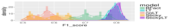
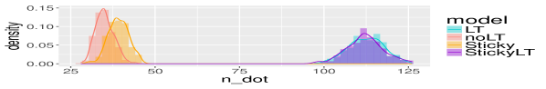
Figure 1: Top: F1 score for inferred relative to ground truth binary speaker matrices on cocktail party data, evaluated every 50th Gibbs iteration after the first 2000, aggregating across 5 runs of each model. Middle: Inferred $\lambda$, for the LT and Sticky-LT models by Gibbs iteration, averaged over 5 runs. Bottom: Number of states used, $n_{\cdot}$, by each model in the training set. Error bands are 99% confidence interval of the mean per iteration.

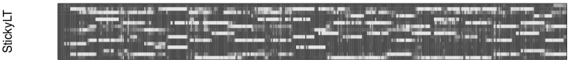
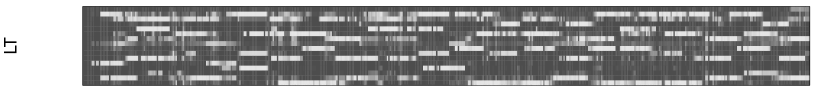
Figure 2: Binary speaker matrices for the cocktail data, with time on the horizontal axis and speaker on the vertical axis. White is 1, black is 0. The ground truth matrix is at the top, followed by the inferred speaker matrix for the Sticky HDP-HMM-LT, HDP-HMM-LT, binary factorial, Sticky-HDP-HMM, and “vanilla” HDP-HMM. All inferred matrices are averaged over 5 runs of 5000 Gibbs iterations each, with the first 2000 iterations discarded as burn-in.

4.2 Synthetic Data Without Local Transitions

We generated data directly from the ordinary HDP-HMM used in the cocktail experiment as a sanity check, to examine the performance of the LT model in the absence of a similarity bias. The results are in Fig. 3. When the $\lambda$ parameter is large, the LT model has worse performance than the non-LT model on this data; however, the $\lambda$ parameter settles near zero as the model learns that local transitions are not more probable. When $\lambda=0$, the HDP-HMM-LT is an ordinary HDP-HMM. The LT model does not make entirely the same inferences as the non-LT model, however; in particular, the $\alpha$ concentration parameter is larger. To some extent, $\alpha$ and $\lambda$ trade off: sparsity of the transition matrix can be achieved either by beginning with a sparse rate matrix prior to rescaling ($\alpha$ small), or by beginning with a less sparse rate matrix which becomes sparser through rescaling (larger $\alpha$ and non-zero $\lambda$).

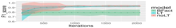
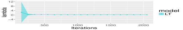
Figure 3: Top: F1 score for inferred relative to ground truth binary speaker matrices on synthetic data generated from the vanilla HDP-HMM model. Middle: Learned similarity parameter, $\lambda$, for the LT model by Gibbs iteration, averaged over 5 runs. Bottom: Number of states used, $n_{\cdot}$, by each model in the training set. Error bands are 99% confidence interval of the mean per iteration. The first 100 iterations are omitted.

4.3 Bach Chorales

To test a version of the HDP-HMM-LT model in which the components of the latent state governing similarity are unrelated to the emission distributions, we used our model to do unsupervised “grammar” learning from a corpus of Bach chorales. The data was a corpus of 217 four-voice major key chorales by J.S. Bach from music21, 200 of which were randomly selected as a training set, with the other 17 used as a test set to evaluate surprisal (marginal log likelihood per observation) by the trained models. All chorales were transposed to C-major, and each distinct four-voice chord (with voices ordered) was encoded as a single integer. In total there were 3307 distinct chord types and 20401 chord tokens in the 217 chorales, with 3165 types and 18818 tokens in the 200 training chorales, and 143 chord types that were unique to the test set.

Modifications to Model and Inference

Since the chords were encoded as integers, the emission distribution for each state is $\mathsf{Cat}(\boldsymbol{\theta}_{j})$. We use a symmetric Dirichlet prior for each $\boldsymbol{\theta}_{j}$, resulting in conjugate updates to $\boldsymbol{\theta}$ conditioned on the latent state sequence, $\mathbf{z}$.

In this experiment, the locations, $\boldsymbol{\ell}_{j}$, are independent of the $\boldsymbol{\theta}_{j}$, with $\mathcal{N}(0,\mathbf{I})$ priors. We use a Gaussian similarity function, $\phi_{jj}:=\exp\{-\lambda d_{2}(\boldsymbol{\ell}_{j},\boldsymbol{\ell}_{j^{\prime}})^{2}\}$ where $d_{2}$ is Euclidean distance. Since the latent states are continuous, we use a Hamiltonian Monte Carlo (HMC) update (Duane et al., 1987; Neal et al., 2011) to update the $\boldsymbol{\ell}_{j}$ simultaneously, conditioned on $\mathbf{z}$ and $\boldsymbol{\pi}$ (see Appendix D for details).

Results

We ran 5 Gibbs chains for 10,000 iterations each using the HDP-HMM-LT, Sticky-HDP-HMM-LT, HDP-HMM and Sticky-HDP-HMM models on the 200 training chorales, which were modeled as conditionally independent of one another. We evaluated the marginal log likelihood on the 17 test chorales (integrating out $\mathbf{z}$) at every 50th iteration. The training and test log likelihoods are in Fig. 4. Although the LT model does not achieve as close a fit to the training data, its generalization performance is better, suggesting that the vanilla HDP-HMM is overfitting. This is perhaps counterintuitive, since the LT model is more flexible, and might be expected to be more prone to overfitting. However, the similarity bias induces greater information sharing across parameters, as in a hierarchical model: instead of each entry of the transition matrix being informed mainly by transitions directly involving the corresponding states, it is informed to some extent by all transitions, as they all inform the similarity structure.

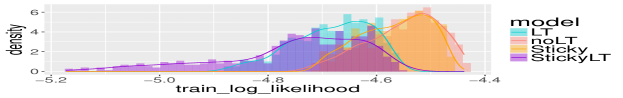
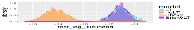
Figure 4: Training set and test set log marginal likelihoods for Bach chorale data on the four HDP-based models: HDP-HMM-LT, HDP-HMM, Sticky HMM, and Sticky HDP-HMM-LT.

5 Discussion

We have defined a new probabilistic model, the Hierarchical Dirichlet Process Hidden Markov Model with Local Transitions (HDP-HMM-LT), which generalizes the HDP-HMM by allowing state space geometry to be represented via a similarity kernel, making transitions between “nearby” pairs of states (“local” transitions), more likely a priori. By introducing an augmented data representation, which we call the Markov Jump Process with Failed Transitions (MJP-FT), we obtain a Gibbs sampling algorithm that simplifies inference in both the LT and ordinary HDP-HMM. When multiple latent chains are interdependent, as in speaker diarization, the HDP-HMM-LT model combines the HDP-HMM’s capacity to discover a small set of joint states with the Factorial HMM’s ability to encode the property that most transitions involve a small number of chains. The HDP-HMM-LT outperforms both, as well as outperforming the Sticky-HDP-HMM, on a speaker diarization task in which speakers form conversational groups. Despite the addition of the similarity kernel, the HDP-HMM-LT is able to suppress its local transition prior when the data does not support it, achieving identical performance to the HDP-HMM on data generated directly from the latter.

The local transition property is particularly clear when transitions occur at different times for different latent features, as with binary vector-valued states in the cocktail party setting, but the model can be used with any state space equipped with a suitable similarity kernel. Similarities need not be defined in terms of emission parameters; state “locations” can be represented and inferred separately, which we demonstrate using Bach chorale data. There, the LT model achieves better predictive performance on a held-out test set, while the ordinary HDP-HMM overfits the training set: the LT property here acts to encourage a concise harmonic representation where chord contexts are arranged in bidirectional functional relationships.

We focused on fixed-dimension binary vectors for the cocktail party and synthetic data experiments, but it would be straightforward to add the LT property to a model with nonparametric latent states, such as the iFHMM (Gael et al., 2009) and the infinite factorial dynamic model (Valera et al., 2015), both of which use the Indian Buffet Process (IBP) (Ghahramani & Griffiths, 2005) as a state prior. The similarity function used here could be employed without changes: since only finitely many coordinates are non-zero in the IBP, the distance between any two states is finite.

Acknowledgments

This work was funded in part by DARPA grant W911NF-14-1-0395 under the Big Mechanism Program and DARPA grant W911NF-16-1-0567 under the Communicating with Computers Program.

APPENDICES

Appendix A concerns the derivation of the augmented data representation referred to as the “Markov Jump Process with Failed Transitions” (MJP-FT). Appendix B fills in details for the Gibbs sampling steps to sample the rescaled HDP used by the HDP-HMM-LT. Appendix C gives a derivation for the updates to the binary state vectors, $\boldsymbol{\theta}$, in the version of the HDP-HMM-LT used in the cocktail party experiment. Finally, appendix D gives the details for the Hamiltonian Monte Carlo update for $\boldsymbol{\ell}$ in the version of the model used in the Bach chorale experiment.

Appendix A Details of the Markov Jump Process with Failed Transitions Representation

We can gain stronger intuition, as well as simplify posterior inference, by re-casting the HDP-HMM-LT as a continuous time Markov Jump Process where some of the attempts to jump from one state to another fail, and where the failure probability increases as a function of the “distance” between the states.

Let $\phi$ be defined as in the last section, and let $\boldsymbol{\beta}$, $\boldsymbol{\theta}$ and $\boldsymbol{\pi}$ be defined as in the Normalized Gamma Process representation of the ordinary HDP-HMM. That is,

$$\boldsymbol{\beta} \sim\mathrm{GEM}(\gamma)$$ (24)

$$\theta_{j} \stackrel{{\scriptstyle i.i.d}}{{\sim}}H$$ (25)

$$\pi_{jj^{\prime}}\,|\,\boldsymbol{\beta},\boldsymbol{\theta} \sim\mathsf{Gamma}(\alpha\beta_{j^{\prime}},1)$$ (26)

Now suppose that when the process is in state $j$, jumps to state $j^{\prime}$ are made at rate $\pi_{jj^{\prime}}$. This defines a continuous-time Markov Process where the off-diagonal elements of the transition rate matrix are the off diagonal elements of $\boldsymbol{\pi}$. In addition, self-jumps are allowed, and occur with rate $\pi_{jj}$. If we only observe the jumps and not the durations between jumps, this is an ordinary Markov chain, whose transition matrix is obtained by appropriately normalizing $\boldsymbol{\pi}$. If we do not observe the jumps themselves, but instead an observation is generated once per jump from a distribution that depends on the state being jumped to, then we have an ordinary HMM.

We modify this process as follows. Suppose that each jump attempt from state $j$ to state $j^{\prime}$ has a chance of failing, which is an increasing function of the “distance” between the states. In particular, let the success probability be $\phi_{jj^{\prime}}$ (recall that we assumed above that $0\leq\phi_{jj^{\prime}}\leq 1$ for all $j,j^{\prime}$). Then, the rate of successful jumps from $j$ to $j^{\prime}$ is $\pi_{jj^{\prime}}\phi_{jj^{\prime}}$, and the corresponding rate of unsuccessful jump attempts is $\pi_{jj^{\prime}}(1-\phi_{jj^{\prime}})$. To see this, denote by $N_{jj^{\prime}}$ the total number of jump attempts to $j^{\prime}$ in a unit interval of time spent in state $j$. Since we are assuming the process is Markovian, the total number of attempts is $\mathsf{Poisson}(\pi_{jj^{\prime}})$ distributed. Conditioned on $N_{jj^{\prime}}$, $n_{jj^{\prime}}$ will be successful, where

$$n_{jj^{\prime}}\,|\,N_{jj^{\prime}}\sim\mathcal{B}\mathrm{inom}(N_{jj^{\prime}},\phi_{jj^{\prime}})$$ (27)

It is easy to show (and well known) that the marginal distribution of $n_{jj^{\prime}}$ is $\mathsf{Poisson}(\pi_{jj^{\prime}}\phi_{jj^{\prime}})$, and the marginal distribution of $\tilde{q}_{jj^{\prime}}:=N_{jj^{\prime}}-n_{jj^{\prime}}$ is $\mathsf{Poisson}(\pi_{jj^{\prime}}(1-\phi_{jj^{\prime}}))$. The rate of successful jumps from state $j$ overall is then $T_{j}:=\sum_{j^{\prime}}\pi_{jj^{\prime}}\phi_{jj^{\prime}}$.

Let $t$ index jumps, so that $z_{t}$ indicates the $t$th state visited by the process (couting self-jumps as a new time step). Given that the process is in state $j$ at discretized time $t-1$ (that is, $z_{t-1}=j$), it is a standard property of Markov Processes that the probability that the first successful jump is to state $j^{\prime}$ (that is, $z_{t}=j^{\prime}$) is proportional to the rate of successful attempts to $j^{\prime}$, which is $\pi_{jj^{\prime}}\phi_{jj^{\prime}}$.

Let $\tilde{u}_{t}$ indicate the time elapsed between the $t$th and and $t-1$th successful jump (where we assume that the first observation occurs when the first successful jump from a distinguished initial state is made). We have

$$\tilde{u}_{t}\,|\,z_{t-1}\sim\mathsf{Exp}(T_{z_{t-1}})$$ (28)

where $\tilde{u}_{t}$ is independent of $z_{t}$.

During this period, there will be $\tilde{q}_{j^{\prime}t}$ unsuccessful attempts to jump to state $j^{\prime}$, where

$$\tilde{q}_{j^{\prime}t}\,|\,z_{t-1}\sim\mathsf{Poisson}(\tilde{u}_{t}\pi_{z_{t-1}j^{\prime}}(1-\phi_{z_{t-1}j^{\prime}}))$$ (29)

Define the following additional variables

$$\mathcal{T}_{j} =\{t\,|\,z_{t-1}=j\}$$ (30)

$$q_{jj^{\prime}} =\sum_{t\in\mathcal{T}_{j}}\tilde{q}_{j^{\prime}t}$$ (31)

$$u_{j} =\sum_{t\in\mathcal{T}_{j}}\tilde{u}_{t}$$ (32)

and let $\mathbf{Q}=(q_{jj^{\prime}})_{j,j^{\prime}\geq 1}$ be the matrix of unsuccessful jump attempt counts, and $\mathbf{u}=(u_{j})_{j\geq 1}$ be the vector of the total times spent in each state.

Since each of the $\tilde{u}_{t}$ with $t\in\mathcal{T}_{j}$ are i.i.d. $\mathsf{Exp}(T_{j})$, we get the marginal distribution

$$u_{j}\,|\,\mathbf{z},\boldsymbol{\pi},\boldsymbol{\phi}\stackrel{{\scriptstyle ind}}{{\sim}}\mathsf{Gamma}(n_{j\cdot},T_{j})$$ (33)

by the standard property that sums of i.i.d. Exponential distributions has a Gamma distribution with shape equal to the number of variates in the sum, and rate equal to the rate of the individual exponentials. Moreover, since the $\tilde{q}_{j^{\prime}t}$ with $t\in\mathcal{T}_{j}$ are Poisson distributed, the total number of failed attempts in the total duration $u_{j}$ is

$$q_{jj^{\prime}}\stackrel{{\scriptstyle ind}}{{\sim}}\mathsf{Poisson}(u_{j}\pi_{jj^{\prime}}(1-\phi_{jj^{\prime}})).$$ (34)

Thus if we marginalize out the individual $\tilde{u}_{t}$ and $\tilde{q}_{j^{\prime}t}$, we have a joint distribution over $\mathbf{z}$, $\mathbf{u}$, and $\mathbf{Q}$, conditioned on the transition rate matrix $\boldsymbol{\pi}$ and the success probability matrix $\boldsymbol{\phi}$, which is

$$p(\mathbf{z},\mathbf{u},\mathbf{Q}\,|\,\boldsymbol{\pi},\boldsymbol{\phi}) =\left(\prod_{t=1}^{T}p(z_{t}\,|\,z_{t-1})\right)\prod_{j}p(u_{j}\,|\,\mathbf{z},\boldsymbol{\pi},\boldsymbol{\phi})\prod_{j^{\prime}}p(q_{jj^{\prime}}\,|\,u_{j}\pi_{jj^{\prime}},\phi_{jj^{\prime}})$$ (35)

$$=\left(\prod_{t}\frac{\pi_{z_{t-1}z_{t}}\phi_{z_{t-1}z_{t}}}{T_{z_{t-1}}}\right)\prod_{j}\frac{T_{j}^{n_{j\cdot}}}{\Gamma(n_{j\cdot})}u_{j}^{n_{j\cdot}-1}e^{-T_{j}u_{j}}$$ (36)

$$\qquad\qquad\times\prod_{j^{\prime}}e^{-u_{j}\pi_{jj^{\prime}}(1-\phi_{jj^{\prime}})}u_{j}^{q_{jj^{\prime}}}\pi_{jj^{\prime}}^{q_{jj^{\prime}}}(1-\phi_{jj^{\prime}})^{q_{jj^{\prime}}}(q_{jj^{\prime}}!)^{-1}$$ (37)

$$=\prod_{j}\Gamma(n_{j\cdot})^{-1}u_{j}^{n_{j\cdot}+q_{j\cdot}-1}$$ (38)

$$\qquad\qquad\times\prod_{j^{\prime}}\pi_{jj^{\prime}}^{n_{jj^{\prime}}+q_{jj^{\prime}}}\phi_{jj^{\prime}}^{n_{jj^{\prime}}}(1-\phi_{jj^{\prime}})^{q_{jj^{\prime}}}e^{-\pi_{jj^{\prime}}\phi_{jj^{\prime}}u_{j}}e^{-\pi_{jj^{\prime}}(1-\phi_{jj^{\prime}})u_{j}}(q_{jj^{\prime}}!)^{-1}$$ (39)

$$=\prod_{j}\Gamma(n_{j\cdot})^{-1}u_{j}^{n_{j\cdot}+q_{j\cdot}-1}\prod_{j^{\prime}}\pi_{jj^{\prime}}^{n_{jj^{\prime}}+q_{jj^{\prime}}}\phi_{jj^{\prime}}^{n_{jj^{\prime}}}(1-\phi_{jj^{\prime}})^{q_{jj^{\prime}}}e^{-\pi_{jj^{\prime}}u_{j}}(q_{jj^{\prime}}!)^{-1}$$ (40)

Setting aside terms that do not depend on $\boldsymbol{\pi}$, we get the conditional likelihood function used in sampling $\boldsymbol{\pi}$:

$$p(\mathbf{z},\mathbf{u},\mathbf{Q}\,|\,\boldsymbol{\pi},\boldsymbol{\phi}) \propto\prod_{j}\prod_{j^{\prime}}\pi_{jj^{\prime}}^{n_{jj^{\prime}}+q_{jj^{\prime}}}e^{-\pi_{jj^{\prime}}u_{j}}$$ (41)

which, combined with the independent Gamma priors on $\pi$ yields conditionally independent Gamma posteriors:

$$\pi_{jj^{\prime}}\,|\,\mathbf{z},\mathbf{u},\mathbf{Q},\boldsymbol{\beta},\alpha\stackrel{{\scriptstyle\text{ind.}}}{{\sim}}\mathsf{Gamma}(\alpha\boldsymbol{\beta}_{j^{\prime}}+n_{jj^{\prime}}+q_{jj^{\prime}},1+u_{j})$$ (42)

Appendix B Inference details for hyperparameters of the rescaled HDP

B.1 Sampling $\boldsymbol{\pi}$, $\boldsymbol{\beta}$, $\alpha$ and $\gamma$

The joint conditional over $\gamma$, $\alpha$, $\boldsymbol{\beta}$ and $\boldsymbol{\pi}$ given the augmented data $\mathcal{D}=(\mathbf{z},\mathbf{u},\mathbf{Q},\mathbf{M},\mathbf{r},w)$ factors as

$$p(\gamma,\alpha,\beta,\pi\,|\,\mathcal{D})=p(\gamma\,|\,\mathcal{D})p(\alpha\,|\,\mathcal{D})p(\beta\,|\,\gamma,\mathcal{D})p(\pi\,|\,\alpha,\beta,\mathcal{D})$$ (43)

We will derive these four factors in reverse order.

Sampling $\boldsymbol{\pi}$

The entries in $\boldsymbol{\pi}$ are conditionally independent given $\alpha$ and $\beta$, so we have the prior

$$p(\boldsymbol{\pi}\,|\,\boldsymbol{\beta},\alpha)=\prod_{j}\prod_{j^{\prime}}\Gamma(\alpha\boldsymbol{\beta}_{j^{\prime}})^{-1}\pi_{jj^{\prime}}^{\alpha\boldsymbol{\beta}_{j^{\prime}}-1}\exp(-\pi_{jj^{\prime}}),$$ (44)

and the likelihood given $\{\mathbf{z},\mathbf{u},\mathbf{Q}\}$ given by (40). Combining these, we have

$$p(\boldsymbol{\pi},\mathbf{z},\mathbf{u},\mathbf{Q}\,|\,\beta,\alpha,\boldsymbol{\phi}) =\prod_{j}u_{j}^{n_{j\cdot}+q_{j\cdot}-1}\prod_{j^{\prime}}\Gamma(\alpha\beta_{j^{\prime}})^{-1}\pi_{jj^{\prime}}^{\alpha\beta_{j^{\prime}}+n_{jj^{\prime}}+q_{jj^{\prime}}-1}$$ (45)

$$\qquad\times e^{-(1+u_{j})\pi_{jj^{\prime}}}\phi_{jj^{\prime}}^{n_{jj^{\prime}}}(1-\phi_{jj^{\prime}})^{q_{jj^{\prime}}}(q_{jj^{\prime}}!)^{-1}$$ (46)

Conditioning on everything except $\boldsymbol{\pi}$, we get

$$p(\boldsymbol{\pi}\,|\,\mathbf{Q},\mathbf{u},\mathbf{z},\boldsymbol{\beta},\alpha) \propto\prod_{j}\prod_{j^{\prime}}\pi_{jj^{\prime}}^{\alpha\beta_{j^{\prime}}+n_{jj^{\prime}}+q_{jj^{\prime}}-1}\exp(-(1+u_{j})\pi_{jj^{\prime}})$$ (47)

and thus we see that the $\pi_{jj^{\prime}}$ are conditionally independent given $u$, $z$ and $Q$, and distributed according to

$$\pi_{jj^{\prime}}\,|\,n_{jj^{\prime}},q_{jj^{\prime}},\beta_{j^{\prime}},\alpha\stackrel{{\scriptstyle ind}}{{\sim}}\mathsf{Gamma}(\alpha\beta_{j^{\prime}}+n_{jj^{\prime}}+q_{jj^{\prime}},1+u_{j})$$ (48)

Sampling $\boldsymbol{\beta}$

Consider the conditional distribution of $\beta$ having integrated out $\boldsymbol{\pi}$. The prior density of $\boldsymbol{\beta}$ is

$$p(\boldsymbol{\beta}\,|\,\gamma)=\frac{\Gamma(\gamma)}{\Gamma(\frac{\gamma}{J})^{J}}\prod_{j}\beta_{j}^{\frac{\gamma}{J}-1}$$ (49)

After integrating out $\pi$ in (45), we have

$$p(\mathbf{z},\mathbf{u},\mathbf{Q}\,|\,\boldsymbol{\beta},\alpha,\gamma,\boldsymbol{\phi}) =\prod_{j=1}^{J}u_{j}^{-1}\prod_{j^{\prime}=1}^{J}u^{n_{jj^{\prime}}+q_{jj^{\prime}}-1}(1+u_{j})^{-(\alpha\beta_{j^{\prime}}+n_{jj^{\prime}}+q_{jj^{\prime}})}$$ (50)

$$\qquad\qquad\times\frac{\Gamma(\alpha\beta_{j^{\prime}}+n_{jj^{\prime}}+q_{jj^{\prime}})}{\Gamma(\alpha\beta_{j^{\prime}})}\phi_{jj^{\prime}}^{n_{jj^{\prime}}}(1-\phi_{jj^{\prime}})^{q_{jj^{\prime}}}(q_{jj^{\prime}}!)^{-1}$$ (51)

$$=\prod_{j=1}^{J}\Gamma(n_{j\cdot})^{-1}u_{j}^{-1}(1+u_{j})^{-\alpha}\left(\frac{u_{j}}{1+u_{j}}\right)^{n_{j\cdot}+q_{j\cdot}}$$ (52)

$$\qquad\qquad\times\prod_{j^{\prime}=1}^{J}\frac{\Gamma(\alpha\beta_{j^{\prime}}+n_{jj^{\prime}}+q_{jj^{\prime}})}{\Gamma(\alpha\beta_{j^{\prime}})}\phi_{jj^{\prime}}^{n_{jj^{\prime}}}(1-\phi_{jj^{\prime}})^{q_{jj^{\prime}}}(q_{jj^{\prime}}!)^{-1}$$ (53)

where we have used the fact that the $\beta_{j}$ sum to 1. Therefore

$$p(\boldsymbol{\beta}\,|\,\mathbf{z},\mathbf{u},\mathbf{Q},\alpha,\gamma) \propto\prod_{j=1}^{J}\beta_{j}^{\frac{\gamma}{J}-1}\prod_{j^{\prime}=1}^{J}\frac{\Gamma(\alpha\beta_{j^{\prime}}+n_{jj^{\prime}}+q_{jj^{\prime}})}{\Gamma(\alpha\beta_{j^{\prime}})}.$$ (54)

Following (Teh et al., 2006), we can write the ratios of Gamma functions as polynomials in $\beta_{j}$, as

$$p(\boldsymbol{\beta}\,|\,\mathbf{z},\mathbf{u},\mathbf{Q},\alpha,\gamma)\propto\prod_{j=1}^{J}\beta_{j}^{\frac{\gamma}{J}-1}\prod_{j^{\prime}=1}^{J}\sum_{m_{jj^{\prime}}=1}^{n_{jj^{\prime}}}s(n_{jj^{\prime}}+q_{jj^{\prime}},m_{jj^{\prime}})(\alpha\beta_{j^{\prime}})^{m_{jj^{\prime}}}$$ (55)

where $s(m,n)$ is an unsigned Stirling number of the first kind, which is used to represent the number of permutations of $n$ elements such that there are $m$ distinct cycles.

This admits an augmented data representation, where we introduce a random matrix $\mathbf{M}=(m_{jj^{\prime}})_{1\leq j,j^{\prime}\leq J}$, whose entries are conditionally independent given $\boldsymbol{\beta}$, $\mathbf{Q}$ and $\mathbf{z}$, with

$$p(m_{jj^{\prime}}=m\,|\,\beta_{j^{\prime}},\alpha,n_{jj^{\prime}},q_{jj^{\prime}})=\frac{s(n_{jj^{\prime}}+q_{jj^{\prime}},m)\alpha^{m}\beta_{j^{\prime}}^{m}}{\sum_{m^{\prime}=0}^{n_{jj^{\prime}}+q_{jj^{\prime}}}s(n_{jj^{\prime}}+q_{jj^{\prime}},m^{\prime})\alpha^{m^{\prime}}\beta_{j^{\prime}}^{m^{\prime}}}$$ (56)

for integer $m$ ranging between $0$ and $n_{jj^{\prime}}+q_{jj^{\prime}}$. Note that $s(n,0)=0$ if $n>0$, $s(0,0)=1$, $s(0,m)=0$ if $m>0$, and we have the recurrence relation $s(n+1,m)=ns(n,m)+s(n,m-1)$, and so we could compute each of these coefficients explicitly; however, it is typically simpler and more computationally efficient to sample from this distribution by simulating the number of occupied tables in a Chinese Restaurant Process with $n$ customers, than it is to enumerate its probabilities.

For each $m_{jj^{\prime}}$ we simply draw $n_{jj^{\prime}}$ assignments of customers to tables according to the Chinese Restaurant Process and set $m_{jj^{\prime}}$ to be the number of distinct tables realized; that is, assign the first customer to a table, setting $m_{jj^{\prime}}$ to 1, and then, after $n$ customers are assigned, assign the $n+1$th customer to a new table with probability $\alpha\beta_{j^{\prime}}/(n+\alpha\beta_{j^{\prime}})$, in which case we increment $m_{jj^{\prime}}$, and to an existing table with probability $n/(n+\alpha)$, in which case we do not increment $m_{jj^{\prime}}$.

Then, we have joint distribution

$$p(\boldsymbol{\beta},\mathbf{M}\,|\,\mathbf{z},\mathbf{u},\mathbf{Q},\alpha,\gamma)\propto\prod_{j=1}^{J}\beta_{j}^{\frac{\gamma}{J}-1}\prod_{j^{\prime}=1}^{J}s(n_{jj^{\prime}}+q_{jj^{\prime}},m_{jj^{\prime}})\alpha^{m_{jj^{\prime}}}\beta_{j^{\prime}}^{m_{jj^{\prime}}}$$ (57)

which yields (55) when marginalized over $\mathbf{M}$. Again discarding constants in $\boldsymbol{\beta}$ and regrouping yields

$$p(\beta\,|\,M,z,u,\theta,\alpha,\gamma)\propto\prod_{{j^{\prime}}=1}^{J}\beta_{j^{\prime}}^{\frac{\gamma}{J}+m_{\cdot{j^{\prime}}}-1}$$ (58)

which is Dirichlet:

$$\beta\,|\,M,\gamma\sim\mathrm{Dirichlet}(\frac{\gamma}{J}+m_{\cdot 1},\dots,\frac{\gamma}{J}+m_{\cdot J})$$ (59)

Sampling $\alpha$ and $\gamma$

Assume that $\alpha$ and $\gamma$ have Gamma priors, parameterized by shape, $a$ and rate, $b$:

$$p(\alpha) =\frac{b_{\alpha}^{a_{\alpha}}}{\Gamma(a_{\alpha})}\alpha^{a_{\alpha}-1}\exp(-b_{\alpha}\alpha)$$ (60)

$$p(\gamma) =\frac{b_{\gamma}^{a_{\gamma}}}{\Gamma(a_{\gamma})}\gamma^{a_{\gamma-1}}\exp(-b_{\gamma}\gamma)$$ (61)

Having integrated out $\boldsymbol{\pi}$, we have

$$p(\boldsymbol{\beta},\mathbf{z},\mathbf{u},\mathbf{Q},\mathbf{M}\,|\,\alpha,\gamma,\boldsymbol{\phi}) =\frac{\Gamma(\gamma)}{\Gamma(\frac{\gamma}{J})^{J}}\alpha^{m_{\cdot\cdot}}\prod_{j=1}^{J}\beta_{j}^{\frac{\gamma}{J}+m_{\cdot j}-1}\Gamma(n_{j\cdot})^{-1}u_{j}^{-1}(1+u_{j})^{-\alpha}\left(\frac{u_{j}}{1+u_{j}}\right)^{n_{j\cdot}+q_{j\cdot}}$$ (62)

$$\qquad\qquad\times\prod_{j^{\prime}=1}^{J}s(n_{jj^{\prime}}+q_{jj^{\prime}},m_{jj^{\prime}})\phi_{jj^{\prime}}^{n_{jj^{\prime}}}(1-\phi_{jj^{\prime}})^{q_{jj^{\prime}}}(q_{jj^{\prime}}!)^{-1}$$ (63)

We can also integrate out $\boldsymbol{\beta}$, to yield

$$p(\mathbf{z},\mathbf{u},\mathbf{Q},\mathbf{M}\,|\,\alpha,\gamma,\boldsymbol{\phi}) =\alpha^{m_{\cdot\cdot}}e^{-\sum_{j^{\prime\prime}}\log(1+u_{j^{\prime\prime}})\alpha}\frac{\Gamma(\gamma)}{\Gamma(\gamma+m_{\cdot\cdot})}$$ (64)

$$\qquad\qquad\times\prod_{j}\frac{\Gamma(\frac{\gamma}{J}+m_{\cdot j})}{\Gamma(\frac{\gamma}{J})\Gamma(n_{j\cdot})}u_{j}^{-1}\left(\frac{u_{j}}{1+u_{j}}\right)^{n_{j\cdot}+q_{j\cdot}}$$ (65)

$$\qquad\qquad\times\prod_{j^{\prime}=1}^{J}s(n_{jj^{\prime}}+q_{jj^{\prime}},m_{jj^{\prime}})\phi_{jj^{\prime}}^{n_{jj^{\prime}}}(1-\phi_{jj^{\prime}})^{q_{jj^{\prime}}}(q_{jj^{\prime}}!)^{-1}$$ (66)

demonstrating that $\alpha$ and $\gamma$ are independent given $\boldsymbol{\phi}$ and the augmented data, with

$$p(\alpha\,|\,\mathbf{z},\mathbf{u},\mathbf{Q},\mathbf{M})\propto\alpha^{a_{\alpha}+m_{\cdot\cdot}}\exp(-(b_{\alpha}+\sum_{j}\log(1+u_{j}))\alpha)$$ (67)

and

$$p(\gamma\,|\,\mathbf{z},\mathbf{u},\mathbf{Q},\mathbf{M}) \propto\gamma^{a_{\gamma-1}}\exp(-b_{\gamma}\gamma)\frac{\Gamma(\gamma)\prod_{j=1}^{J}\Gamma(\frac{\gamma}{J}+m_{\cdot j})}{\Gamma(\frac{\gamma}{J})^{J}\Gamma(\gamma+m_{\cdot\cdot})}$$ (68)

So we see that

$$\alpha\,|\,\mathbf{z},\mathbf{u},\mathbf{Q},\mathbf{M}\sim\mathsf{Gamma}(a_{\alpha}+m_{\cdot\cdot},b_{\alpha}+\sum_{j}\log(1+u_{j}))$$ (69)

To sample $\gamma$, we introduce a new set of auxiliary variables, $\mathbf{r}=(r_{1},\dots,r_{J})$ and $w$ with the following distributions:

$$p(r_{j^{\prime}}=r\,|\,m_{\cdot{j^{\prime}}},\gamma) =\frac{\Gamma(\frac{\gamma}{J})}{\Gamma(\frac{\gamma}{J}+m_{\cdot{j^{\prime}}})}s(m_{\cdot{j^{\prime}}},r)\left(\frac{\gamma}{J}\right)^{r}\qquad r=1,\dots,m_{\cdot j}$$ (70)

$$p(w\,|\,m_{\cdot\cdot}\gamma) =\frac{\Gamma(\gamma+m_{\cdot\cdot})}{\Gamma(\gamma)\Gamma(m_{\cdot\cdot})}w^{\gamma-1}(1-w)^{m_{\cdot\cdot}-1}\qquad w\in(0,1)$$ (71)

so that

$$p(\gamma,r,w\,|\,\mathbf{M}) \propto\gamma^{a_{\gamma-1}}\exp(-b_{\gamma}\gamma)w^{\gamma-1}(1-w)^{m_{\cdot\cdot}-1}\prod_{j^{\prime}=1}^{J}s(m_{\cdot{j^{\prime}}},r_{j^{\prime}})\left(\frac{\gamma}{J}\right)^{r_{j^{\prime}}}$$ (72)

and

$$p(\gamma\,|\,r,w)\propto\gamma^{a_{\gamma}+r_{\cdot}-1}\exp(-(b_{\gamma}-\log(w))\gamma),$$ (73)

which is to say

$$\gamma\,|\,\mathbf{r},w,\mathbf{z},\mathbf{u},\mathbf{Q},\mathbf{M}\sim\mathsf{Gamma}(a_{\gamma}+r_{\cdot},b_{\gamma}-\log(w))$$ (74)

Appendix C Derivation of $\boldsymbol{\eta}$ update in the Cocktail Party and Synthetic Data Experiments

In principle, $\boldsymbol{\eta}$ can have any distribution over binary vectors, but we will suppose for simplicity that it can be factored into $D$ independent coordinate-wise Bernoulli variates. Let $\mu_{d}$ be the Bernoulli parameter for the $d$th coordinate.

The similarity function $\phi_{jj^{\prime}}$ is the Laplacian kernel:

$$\phi_{jj^{\prime}} =\Phi(\boldsymbol{\eta}_{j},\boldsymbol{\eta}_{j^{\prime}})=\exp(-\lambda d_{jj^{\prime}})$$ (75)

where $d_{jj^{\prime}d}=\left|\boldsymbol{\eta}_{jd}-\boldsymbol{\eta}_{j^{\prime}d}\right|$ is Hamming distance in the $d$th coordinate, $d_{jj^{\prime}}:=\sum_{d=1}^{D}d_{jj^{\prime}}$ is the total Hamming distance between $\boldsymbol{\eta}_{j}$ and $\boldsymbol{\eta}_{j^{\prime}}$, and $\lambda\geq 0$ (if $\lambda=0$, the $\phi_{jj^{\prime}}$ are identically 1, and so do not have any influence, reducing the model to an ordinary HDP-HMM).

Let

$$\phi_{jj^{\prime}-d} =\exp(-\lambda(d_{jj^{\prime}}-d_{jj^{\prime}d}))$$ (76)

so that $\phi_{jj^{\prime}}=\phi_{jj^{\prime}-d}e^{-\lambda d_{jj^{\prime}d}}$.

Since the matrix $\boldsymbol{\phi}$ is assumed to be symmetric, we have

$$\frac{p(\mathbf{z},\mathbf{Q}\,|\,\eta_{jd}=1,\boldsymbol{\eta}\setminus\eta_{jd})}{p(\mathbf{z},\mathbf{Q}\,|\,\eta_{jd}=0,\boldsymbol{\eta}\setminus\eta_{jd})} \propto\prod_{j^{\prime}\neq j}\frac{e^{-\lambda(n_{jj^{\prime}}+n_{j^{\prime}j})\left|1-\theta_{j^{\prime}d}\right|}(1-\phi_{jj^{\prime}-d}e^{-\lambda\left|1-\theta_{j^{\prime}d}\right|})^{q_{jj^{\prime}}+q_{j^{\prime}j}}}{e^{-\lambda(n_{jj^{\prime}}+n_{j^{\prime}j})\left|\theta_{j^{\prime}d}\right|}(1-\phi_{jj^{\prime}-d}e^{-\lambda\left|\theta_{j^{\prime}d}\right|})^{q_{jj^{\prime}}+q_{j^{\prime}j}}}$$ (77)

$$=e^{-\lambda(c_{jd0}-c_{jd1})}\prod_{j^{\prime}\neq j}\left(\frac{1-\phi_{jj^{\prime}-d}e^{-\lambda}}{1-\phi_{jj^{\prime}-d}}\right)^{(-1)^{\theta_{j^{\prime}d}}(q_{jj^{\prime}}+q_{j^{\prime}j})}$$ (78)

where $c_{jd0}$ and $c_{jd1}$ are the number of successful jumps to or from state $j$, to or from states with a 0 or 1, respectively, in position $d$. That is,

$$c_{jd0}=\sum_{\{j^{\prime}\,|\,\theta_{j^{\prime}d}=0\}}n_{jj^{\prime}}+n_{j^{\prime}j}\qquad c_{jd1}=\sum_{\{j^{\prime}\,|\,\theta_{j^{\prime}d}=1\}}n_{jj^{\prime}}+n_{j^{\prime}j}$$ (79)

Therefore, we can Gibbs sample $\eta_{jd}$ from its conditional posterior Bernoulli distribution given the rest of $\boldsymbol{\eta}$, where we compute the Bernoulli parameter via the log-odds

$$\log\left(\frac{p(\eta_{jd}=1\,|\,\mathbf{Y},\mathbf{z},\mathbf{Q},\boldsymbol{\eta}\setminus\eta_{jd})}{p(\eta_{jd}=0\,|\,\mathbf{Y},\mathbf{z},\mathbf{Q},\boldsymbol{\eta}\setminus\eta_{jd})}\right)=\log\left(\frac{p(\eta_{jd}=1)p(\mathbf{z},\mathbf{Q}\,|\,\eta_{jd}=1,\boldsymbol{\eta}\setminus\eta_{jd})p(\mathbf{Y}\,|\,\mathbf{z},\eta_{jd}=1,\boldsymbol{\eta}\setminus\eta_{jd})}{p(\eta_{jd}=0)p(\mathbf{z},\mathbf{Q}\,|\,\eta_{jd}=0,\boldsymbol{\eta}\setminus\eta_{jd})p(\mathbf{Y}\,|\,\mathbf{z},\eta_{jd}=0,\boldsymbol{\eta}\setminus\eta_{jd})}\right)$$ (80)

$$\qquad=\log\left(\frac{\mu_{d}}{1-\mu_{d}}\right)+(c_{jd1}-c_{jd0})\lambda+\sum_{j^{\prime}\neq j}(-1)^{\theta_{j^{\prime}d}}(q_{jj^{\prime}}+q_{j^{\prime}j})\log\left(\frac{1-\phi_{jj^{\prime}}^{(-d)}e^{-\lambda}}{1-\phi_{jj^{\prime}}^{(-d)}}\right)$$ (81)

$$\qquad\qquad+\sum_{\{t\,|\,z_{t}=j\}}\log\left(\frac{f(\mathbf{y}_{t};\eta_{jd}=1,\boldsymbol{\eta}_{j}\setminus\eta_{jd})}{f(\mathbf{y}_{t};\eta_{jd}=0,\boldsymbol{\eta}_{j}\setminus\eta_{jd})}\right)$$ (82)

Suppose also that the observed data $\mathbf{Y}$ consists of a $T\times K$ matrix, where the $t$th row $\mathbf{y}_{t}=(y_{t1},\dots,y_{tK})^{\mathsf{T}}$ is a $K$-dimensional feature vector associated with time $t$, and let $\mathbf{W}$ be a $D\times K$ weight matrix with $k$th column $\mathbf{w}_{k}$, such that

$$f(\mathbf{y}_{t};\boldsymbol{\eta}_{j})=g(\mathbf{y}_{t};\mathbf{W}^{\mathsf{T}}\boldsymbol{\eta}_{j})$$ (83)

for a suitable parametric function $g$. We assume for simplicity that $g$ factors as

$$g(\mathbf{y}_{t};\mathbf{W}^{\mathsf{T}}\boldsymbol{\eta}_{j})=\prod_{k=1}^{K}g_{k}(y_{tk};\mathbf{w}_{k}\cdot\boldsymbol{\eta}_{j})$$ (84)

Define $x_{tk}=\mathbf{w}_{k}\cdot\theta_{z_{t}}$, and $x_{tk}^{(-d)}=\mathbf{w}_{k}^{-d}\cdot\theta_{z_{t}}^{-d}$, where $\theta_{j}^{-d}$ and $\mathbf{w}_{k}^{-d}$ are $\theta_{j}$ and $\mathbf{w}_{k}$, respectively, with the $d$th coordinate removed. Then

$$\log\left(\frac{f(\mathbf{y}_{t};\eta_{jd}=1,\boldsymbol{\eta}_{j}\setminus\eta_{jd})}{f(\mathbf{y}_{t};\eta_{jd}=0,\boldsymbol{\eta}_{j}\setminus\eta_{jd})}\right)=\sum_{k=1}^{K}\log\left(\frac{g_{k}(y_{tk};x_{tk}^{(-d)}+w_{dk})}{g_{k}(y_{tk};x_{tk}^{(-d)})}\right).$$ (85)

If $g_{k}(y;x)$ is a Normal density with mean $x$ and unit variance, then

$$\log\left(\frac{g_{k}(y_{tk};x_{tk}^{(-d)}+w_{dk})}{g_{k}(y_{tk};x_{tk}^{(-d)})}\right)=-w_{dk}(y_{tk}-x_{tk}^{(-d)}+\frac{1}{2}w_{dk})$$ (86)

Appendix D Derivation of HMC update for $\boldsymbol{\ell}$ in the Bach Chorale Experiment

We have a set of states with parameters $\boldsymbol{\ell}_{j}$, $j=1,\dots,J$. In the previous version of the model, $\boldsymbol{\ell}_{j}$ was a binary state vector on which both the similarities $\phi_{jj^{\prime}}$ and the emission distribution $F_{j}$ depended. Here, we define the latent locations $\boldsymbol{\ell}_{j}=(\ell_{j1},\ell_{jD})$ to be locations in $\mathbb{R}^{D}$, independent of the emission distributions, so that during inference they are informed solely by the transitions.

We set

$$\phi_{jj^{\prime}}(\boldsymbol{\ell}_{j},\boldsymbol{\ell}_{j^{\prime}})=\exp\left(-\frac{\lambda}{2}d_{jj^{\prime}}^{2}\right)$$

where $d_{jj^{\prime}}$ is the Euclidean distance between $\boldsymbol{\ell}_{j}$ and $\boldsymbol{\ell}_{j^{\prime}}$; that is,

$$d_{jj^{\prime}}^{2}=\sum_{d}(\ell_{jd}-\ell_{j^{\prime}d})^{2}$$

Since now $\boldsymbol{\ell}_{j}$ are continuous locations, we use Hamlitonian Monte Carlo (Duane et al., 1987; Neal et al., 2011) to sample them jointly. HMC is a variation on Metropolis-Hastings algorithm which is designed to more efficiently explore a high-dimensional continuous distribution by adopting a proposal distribution which incorporates an auxiliary “momentum” variable to make it more likely that proposals will go in useful directions and improve mixing compared to naive movement.

To do Hamiltonian Monte Carlo to sample from the conditional posterior of $\boldsymbol{\ell}$ given $\mathbf{z}$ and $\mathbf{Q}$, we need to compute the gradient of the log posterior, which is just the sum of the gradient of the log prior and the gradient of the log likelihood.

Assume independent and isotropic Gaussian priors on each $\boldsymbol{\ell}_{j}$, so we have

$$p(\boldsymbol{\ell}_{j})\propto\exp\left(-\frac{h_{\ell}}{2}\sum_{d}\ell_{jd}^{2}\right),$$

where $h_{\ell}$ is the prior precision which does not depend on $d$.

Then the log prior density, up to an additive constant $c$, is

$$\log p(\boldsymbol{\ell}_{j})=c-\frac{h_{\ell}}{2}\sum_{d}\ell_{jd}^{2}$$

The relevant log likelihood is the log of the probability of the $\mathbf{z}$ and $\mathbf{Q}$ variables given the $\phi_{jj^{\prime}}$. In particular, we have

$$L:=p(\mathbf{z},\mathbf{Q}\,|\,\boldsymbol{\phi})\propto\prod_{j}\prod_{j^{\prime}}\phi_{jj^{\prime}}^{n_{jj^{\prime}}}(1-\phi_{jj^{\prime}})^{q_{jj^{\prime}}}$$

so that

$$\log L=\sum_{j}\sum_{j^{\prime}}\left(n_{jj^{\prime}}\log(\phi_{jj^{\prime}})+q_{jj^{\prime}}\log(1-\phi_{jj^{\prime}})\right)$$

The $j,d$ coordinate of the gradient of the log prior is simply $-h_{\ell}\ell_{jd}$.

To get the $j,d$ coordinate of the gradient of the log likelihood, we can apply the chain rule to terms as is convenient. In particular,

$$\frac{\partial L}{\partial\ell_{jd}}=\sum_{j}\sum_{j^{\prime}}n_{jj^{\prime}}\frac{\partial\log(\phi_{jj^{\prime}})}{\partial d_{jj^{\prime}}^{2}}\frac{\partial d_{jj^{\prime}}^{2}}{\partial\ell_{jd}}+\sum_{j}\sum_{j^{\prime}}q_{jj^{\prime}}\frac{\partial\log(1-\phi_{jj^{\prime}})}{\partial(1-\phi_{jj^{\prime}})}\frac{\partial(1-\phi_{jj^{\prime}})}{\partial d_{jj^{\prime}}^{2}}\frac{\partial d_{jj^{\prime}}^{2}}{\partial\ell_{jd}}$$

We have the following components:

$$\frac{\partial\log(\phi_{jj^{\prime}})}{\partial d_{jj^{\prime}}^{2}} =-\frac{\lambda}{2}$$

$$\frac{\partial d_{jj^{\prime}}^{2}}{\partial\ell_{jd}} =2d_{jj^{\prime}d}I(j\neq j^{\prime})$$

$$\frac{\partial\log(1-\phi_{jj^{\prime}})}{\partial(1-\phi_{jj^{\prime}})} =\frac{1}{1-\phi_{jj^{\prime}}}$$

$$\frac{\partial(1-\phi_{jj^{\prime}})}{\partial d_{jj^{\prime}}^{2}} =\frac{\lambda}{2}\phi_{jj^{\prime}}$$

which yields

$$\frac{\partial L}{\partial\ell_{jd}} =-\lambda\sum_{j}\sum_{j^{\prime}}n_{jj^{\prime}}d_{jj^{\prime}d}\mathbb{I}(j\neq j^{\prime})+\lambda\sum_{j}\sum_{j^{\prime}}q_{jj^{\prime}}d_{jj^{\prime}d}\frac{\phi_{jj^{\prime}}}{1-\phi_{jj^{\prime}}}\mathbb{I}(j\neq j)$$

$$=-\lambda\sum_{(j,j^{\prime}):j\neq j^{\prime}}d_{jj^{\prime}d}\left(n_{jj^{\prime}}-q_{jj^{\prime}}\frac{\phi_{jj^{\prime}}}{1-\phi_{jj^{\prime}}}\right)$$

References

- Beal et al. (2001) Beal, Matthew J, Ghahramani, Zoubin, and Rasmussen, Carl E. The infinite hidden Markov model. In Advances in neural information processing systems, pp. 577–584, 2001.
- Duane et al. (1987) Duane, Simon, Kennedy, Anthony D, Pendleton, Brian J, and Roweth, Duncan. Hybrid monte carlo. Physics letters B, 195(2):216–222, 1987.
- Ewens (1990) Ewens, Warren John. Population genetics theory – the past and the future. In Mathematical and Statistical Developments of Evolutionary Theory, pp. 177–227. Springer, 1990.
- Favaro et al. (2013) Favaro, Stefano, Teh, Yee Whye, et al. MCMC for normalized random measure mixture models. Statistical Science, 28(3):335–359, 2013.
- Ferguson (1973) Ferguson, Thomas S. A Bayesian analysis of some nonparametric problems. The annals of statistics, pp. 209–230, 1973.
- Fox et al. (2008) Fox, Emily B, Sudderth, Erik B, Jordan, Michael I, and Willsky, Alan S. An HDP-HMM for systems with state persistence. In Proceedings of the 25th international conference on Machine learning, pp. 312–319. ACM, 2008.
- Gael et al. (2009) Gael, Jurgen V, Teh, Yee W, and Ghahramani, Zoubin. The infinite factorial hidden Markov model. In Advances in Neural Information Processing Systems, pp. 1697–1704, 2009.
- Ghahramani & Griffiths (2005) Ghahramani, Zoubin and Griffiths, Thomas L. Infinite latent feature models and the Indian buffet process. In Advances in neural information processing systems, pp. 475–482, 2005.
- Ghahramani et al. (1997) Ghahramani, Zoubin, Jordan, Michael I, and Smyth, Padhraic. Factorial hidden Markov models. Machine learning, 29(2-3):245–273, 1997.
- Gilks & Wild (1992) Gilks, Walter R and Wild, Pascal. Adaptive rejection sampling for Gibbs sampling. Applied Statistics, pp. 337–348, 1992.
- Ishwaran & Zarepour (2002) Ishwaran, Hemant and Zarepour, Mahmoud. Exact and approximate sum representations for the Dirichlet process. Canadian Journal of Statistics, 30(2):269–283, 2002.
- Johnson & Willsky (2013) Johnson, Matthew J and Willsky, Alan S. Bayesian nonparametric hidden semi-Markov models. The Journal of Machine Learning Research, 14(1):673–701, 2013.
- Kingman (1967) Kingman, John. Completely random measures. Pacific Journal of Mathematics, 21(1):59–78, 1967.
- Neal et al. (2011) Neal, Radford M et al. MCMC using Hamiltonian dynamics. Handbook of Markov Chain Monte Carlo, 2:113–162, 2011.
- Paisley et al. (2012) Paisley, John, Wang, Chong, and Blei, David M. The discrete infinite logistic normal distribution. Bayesian Analysis, 7(4):997–1034, 2012.
- Ranganath & Blei (2016) Ranganath, Rajesh and Blei, David M. Correlated random measures. Journal of the American Statistical Association, 2016.
- Sethuraman (1994) Sethuraman, Jayaram. A constructive definition of Dirichlet processes. Statistica Sinica, 4:639–650, 1994.
- Teh et al. (2006) Teh, Yee Whye, Jordan, Michael I, Beal, Matthew J, and Blei, David M. Hierarchical Dirichlet processes. Journal of the American Statistical Association, 101(476), 2006.
- Valera et al. (2015) Valera, Isabel, Ruiz, Francisco, Svensson, Lennart, and Perez-Cruz, Fernando. Infinite factorial dynamical model. In Advances in Neural Information Processing Systems, pp. 1657–1665, 2015.
- Van Gael et al. (2008) Van Gael, Jurgen, Saatci, Yunus, Teh, Yee Whye, and Ghahramani, Zoubin. Beam sampling for the infinite hidden Markov model. In Proceedings of the 25th International Conference on Machine Learning, pp. 1088–1095. ACM, 2008.
- Zhu et al. (2016) Zhu, Hao, Hu, Jinsong, and Leung, Henry. Hidden Markov models with discrete infinite logistic normal distribution priors. In Information Fusion (FUSION), 2016 19th International Conference on, pp. 429–433. IEEE, 2016.