Reanalysis of the BICEP2, Keck and Planck Data: No Evidence for Gravitational Radiation

Abstract

A joint analysis of data collected by the Planck and BICEP2+Keck teams has previously given $r=0.09^{+0.06}_{-0.04}$ for BICEP2 and $r=0.02^{+0.04}_{-0.02}$ for Keck. Analyzing BICEP2 using its published noise estimate, we had earlier (Colley & Gott 2015) found $r=0.09\pm 0.04$, agreeing with the final joint results for BICEP2. With the Keck data now available, we have done something the joint analysis did not: a correlation study of the BICEP2 vs. Keck B-mode maps. Knowing the correlation coefficient between the two and their amplitudes allows us to determine the noise in each map (which we check using the E-modes). We find the noise power in the BICEP2 map to be twice the original BICEP2 published estimate, explaining the anomalously high $r$ value obtained by BICEP2. We now find $r=0.004\pm 0.04$ for BICEP2 and $r=-0.01\pm 0.04$ for Keck. Since $r\geq 0$ by definition, this implies a maximum likelihood value of $r=0$, or no evidence for gravitational waves. Starobinsky Inflation ($r=0.0036$) is not ruled out, however.

Krauss & Wilzcek (2014) have already argued that “measurement of polarization of the CMB due to a long-wavelength stochastic background of gravitational waves from Inflation in the early Universe would firmly establish the quantization of gravity,” and, therefore, the existence of gravitons. We argue it would also constitute a detection of gravitational Hawking radiation (explicitly from the causal horizons due to Inflation).

1 Introduction

The BICEP2 team announced discovery of B polarization modes on angular scales of $1^{\circ}$ to $5^{\circ}$ ($l=40$ to $l=200$), which they claimed were of an amplitude and angular scale that are too large to be due to gravitational lensing (BICEP2 Collaboration 2014). They claimed a power in B-modes corresponding to a tensor-to-scalar ratio of $r=0.2$ as compared with a value of $r=0.13$ expected from simple single-field slow-roll chaotic inflation (Linde 1983) with a simple quadratic potential $V(\phi)=(1/2)m^{2}\phi^{2}$ representing a simple massive scalar field (with mass $m$), assuming dust contamination was negligible. They estimated that dust contamination could at most lower $r$ by 0.04 to a value of $r=0.16\pm 0.04$. The main question appeared to be whether the B-modes could instead be due entirely to B-modes produced by foreground dust. Mortonson, and Seljak (2014) and Flauger, Hill & Spergel (2014) immediately argued that given the uncertainties of the amplitude of the dust polarization at the BICEP2 frequency of 150 GHz, one cannot say conclusively at present whether the B-modes detected by BICEP2 are due to gravitational waves or just polarized dust. All of these studies looked only the power spectrum of the B-modes. Flauger, Hill & Spergel (2014) in particular, fitting the B-mode power spectrum on the $1^{\circ}$ to $5^{\circ}$ scale, found that a model with $r=0.2$ and no appreciable dust polarization ($\chi^{2}=1.1$) is acceptable, as well as a model with $r=0$ and dust B-modes ($\chi^{2}=1.7$). They thus concluded that given the present uncertainty in the amplitude of the dust emission B-modes at 150 GHz one cannot say at present whether the BICEP2 B-modes are due to gravitational waves or dust polarization. Flauger, Hill & Spergel digitized a publicly available Planck polarization map to compare with the BICEP2 map. We similarly digitized and utilized this publicly available Planck polarization map in a previous study (Colley & Gott 2015). In that work, we conducted a correlation study between BICEP2 and Planck in the B-mode maps to determine the amount of dust contamination. The power in the B-modes came from several sources which gave fractional contributions of $x$ (primordial gravitational waves), $y$ (dust contamination), $z$ (gravitational lensing), and $w$ (noise). These added to unity. We used the correlation coefficient between the BICEP2 and Planck maps to estimate the value of $y$. The value of $z$ came from simulations (quoted by BICEP2), and the value of $w$ was taken from the estimate provided by the BICEP2 team. By subtraction, we could determine the value of $x$ and given the amplitude of the BICEP2 map we could determine the value of $r$. We showed that a variety of mapping techniques all gave similar results for $r$ within the errors. With the optimal tapered map (which the joint analysis would later adopt), and which gave the largest correlation coefficient between the BICEP2 and Planck maps, we found $r=0.099\pm 0.04$ (Colley & Gott 2015). We found a larger amount of dust contamination than BICEP2 estimated, but still not enough to explain the data without a barely significant ($2\sigma$) detection of gravitational waves. Importantly, we used the noise estimate $w$ provided by the BICEP2 team, the only one available, which no one had questioned. When we say noise we, of course, mean antenna noise plus any systematic errors in the BICEP2 map. We will always just refer to this as noise.

Then, shortly after our paper appeared, the BICEP2 + Planck teams published their joint analysis. The value they obtained for BICEP2 was $r=0.09^{+0.06}_{-0.04}$. They did this using a power spectrum analysis. They found essentially identical results to what we found using a direct correlation analysis of the BICEP2 and Planck maps. We used the Planck map, as did they, in the standard way to estimate the dust contamination power in the B-modes ($y$) by using the Planck map (taken at $353\mbox{GHz}$) to estimate the amplitude of the dust modes at 150 GHz where BICEP2 observed. We would emphasize that our results were essentially equivalent to those found by the joint analysis of BICEP2 and Planck by their teams. So far so good. But a new, and unexpected addition appeared in the joint analysis: new, previously unpublished Keck data was added to the mix. The joint analysis of Keck versus Planck gave $r=0.02^{+0.04}_{-0.02}$. The Keck data suggested a much lower value of $r$ than BICEP2. The two results were surprisingly different (at the $1.75\sigma$) level. The joint analysis regarded both Keck and BICEP2 as equally accurate, and weighing them equally found a final answer $r=0.05\pm 0.04$. Their paper concluded that the Keck and BICEP2 data were comparable and the final answer was basically the average of the two maps. This was not a significant detection at the $2\sigma$ level. The headline was that the original claimed detection of gravitational waves by BICEP2 had been done in by dust contamination.

Actually, when they analyzed BICEP2 alone, they still found a significant level of gravitational waves, even when the dust was properly accounted for. What did in the BICEP2 detection was actually the new Keck data which suggested a very low value for gravitational waves, less than $1\sigma$ above zero. Left unresolved was the question of why the BICEP2 results were so different from the Keck results. Also, their final best answer using both Keck and BICEP2 for gravitational waves was still positive at about $1.25\sigma$—not enough to be significant at the $2\sigma$ level, but still giving some weak evidence for gravitational waves, since including some gravitational waves still gave a better fit to all the data according to their analysis, than assuming gravitational waves were absent. A subsequent paper, adding still more new data at a frequency of $90\mbox{GHz}$ to further evaluate the dust signal led them to a $2\sigma$ upper limit of $r=0.07$, only slightly improving their original joint analysis $2\sigma$ upper limit of $r=0.09$.

In this paper we will do something the joint analysis did not do: we will do a direct correlation analysis of the BICEP2 versus Keck maps (both at $150\mbox{GHz}$) to determine the true noise levels in both maps. We will then use these values to determine the value of $r$ implied by BICEP2 and Keck independently. Surprisingly, we will find that the noise power published in the original BICEP2 paper was low by a factor of two. We check our noise estimates for BICEP2 and Keck by predicting the correlation coefficient we expect for the (higher amplitude) E-mode maps and finding it agrees with what we actually observe. Using the correct noise estimates for BICEP2 and Keck we will find both give estimates for $r$ consistent with zero, implying no evidence for gravitational waves.

2 Correlation Coefficient between BICEP2 and Keck B-mode Maps

The rms amplitude of the B mode map for BICEP2 is $\sigma_{B}=0.0829\mu\mbox{K}$, from our digitized map. The method we used for digitizing the B-mode BICEP2 map is given in detail in Colley and Gott (2015). For the B-mode maps from BICEP2 we find

$$\sigma_{B}^{2}=\sigma_{BGW}^{2}+\sigma_{BN}^{2}+\sigma_{BGL}^{2}+\sigma_{BD}^{2},$$ (1)

where $\sigma_{BGW}$ is the standard deviation of the BICEP2 gravitational wave signal, $\sigma_{BN}$ is the standard deviation of the BICEP2 noise, $\sigma_{BGL}$ is the standard deviation of BICEP2 gravitational lensing signal, and $\sigma_{BD}$ is the standard deviation of the BICEP2 dust signal (since all these are uncorrelated with each other). The BICEP2 team has produced a simulation showing only the expected gravitational lensing and noise. From our digitization of the BICEP2 simulation map, which includes only gravitational lensing and noise, we find its $1\sigma$ amplitude to be $\sigma_{sim}=0.0547\mu\mbox{K}=0.660\sigma_{B}$. The simulation has an amplitude $\sigma_{sim}^{2}=\sigma_{BN}^{2}+\sigma_{BGL}^{2}=[0.0547\mu\mbox{K}]^{2}=0.435\sigma_{B}^{2}$.

Let us begin by defining some terms:

$$x =\sigma_{BGW}^{2}/\sigma_{B}^{2}$$ (2)

$$y =\sigma_{BD}^{2}/\sigma_{B}^{2}$$

$$z =\sigma_{BGL}^{2}/\sigma_{B}^{2}$$

$$w =\sigma_{BN}^{2}/\sigma_{B}^{2}$$

$$1 =x+y+z+w.$$

A direct measurement of $z=0.195$ is made from the BICEP2 paper showing the standard simulation of gravitational lensing–measured directly from their figure. Knowing that $w+z=0.435$, from measurement of the amplitude of their simulation map (without gravitational waves or dust), we found, using the estimates in the BICEP paper that $w=0.24$. That is the noise power estimated by the BICEP2 team. But we will not be using that value here. We will deduce it from a correlation analysis with the independent Keck data (taken by the same BICEP2 team members with a different telescope at the same south pole site).

We establish similar variables for the Keck B-mode map. For both BICEP2 and Keck we will use identical tapered maps (like our map IV in Colley & Gott [2015]). This tapered map, going smoothly to zero amplitude at the outer boundary, is designed to minimize the confusion between E and B-modes in the polarization data, and is exactly the type of map used by the joint analysis by the Planck and BICEP2 teams. For the Keck data we define:

$$x^{\prime} =\sigma_{BGW}^{2}/\sigma_{K}^{2}$$ (3)

$$y^{\prime} =\sigma_{BD}^{2}/\sigma_{K}^{2}$$

$$w^{\prime} =\sigma_{BN}^{2}/\sigma_{K}^{2}$$

$$1 =x^{\prime}+y^{\prime}+z^{\prime}+w^{\prime}.$$

Thus, the primed values refer to the Keck B-mode map and the unprimed values refer to the BICEP2 map, where $\sigma_{K}$ is the rms amplitude of the Keck map. Both maps include only modes with $50<l<120$. Both B-mode maps are at $150\mbox{GHz}$ and so have equal signals in gravitational waves, dust, and gravitational lensing: $\sigma_{BGW}^{2}=\sigma_{KGW}^{2}$, $\sigma_{BD}^{2}=\sigma_{KD}^{2}$, $\sigma_{BGL}^{2}=\sigma_{KGL}^{2}$ because they are looking at the same piece of sky. These are correlated signals in both maps, while the noise in the maps is uncorrelated. Thus, the correlation coefficient between the BICEP2 and Keck maps is:

$$C =(\sigma_{BGW}\sigma_{KGW}+\sigma_{BD}\sigma_{KD}+\sigma_{BGL}\sigma_{KGL})/\sigma_{B}\sigma_{K}$$ (4)

$$C =(\sigma_{BGW}^{2}+\sigma_{BD}^{2}+\sigma_{BGL}^{2})/(\sigma_{B}\sigma_{K})$$

$$=(\sigma_{KGW}^{2}+\sigma_{KD}^{2}+\sigma_{KGL}^{2})/(\sigma_{B}\sigma_{K})$$

$$C =(\sigma_{B}^{2}-\sigma_{BN}^{2})/(\sigma_{B}\sigma_{K})$$

$$=(\sigma_{K}^{2}-\sigma_{KN}^{2})/(\sigma_{B}\sigma_{K}).$$

So, solving for the noise amplitudes we find:

$$\sigma_{BN}^{2}=\sigma_{B}^{2}-C\sigma_{B}\sigma_{K}$$ (5)

and

$$\sigma_{KN}^{2}=\sigma_{K}^{2}-C\sigma_{B}\sigma_{K}.$$ (6)

The Keck and BICEP2 B-mode maps are shown together in Fig. 1; they have a correlation coefficient of $C=0.566$, which is surprisingly small.

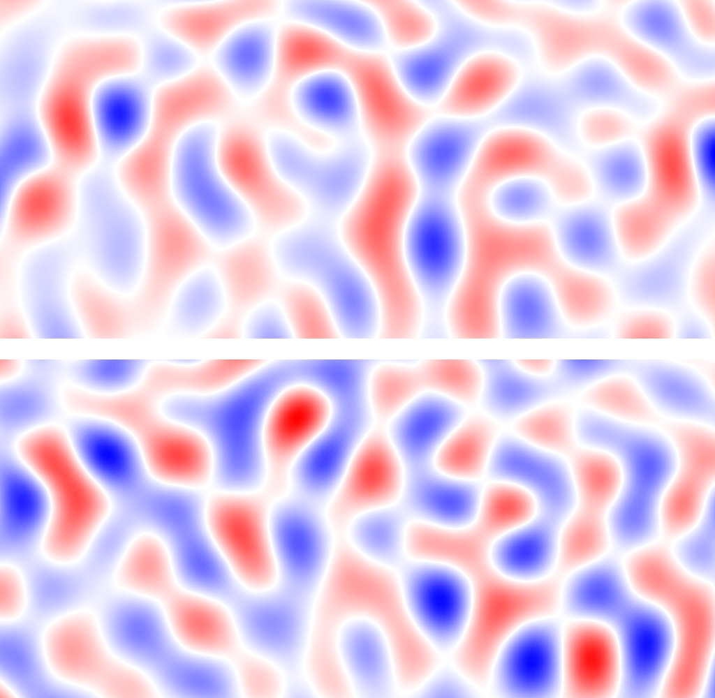
Figure 1: Correlation of BICEP2 (bottom) and Keck (top) B-mode polarization maps. The correlation coefficient $C=0.566$.

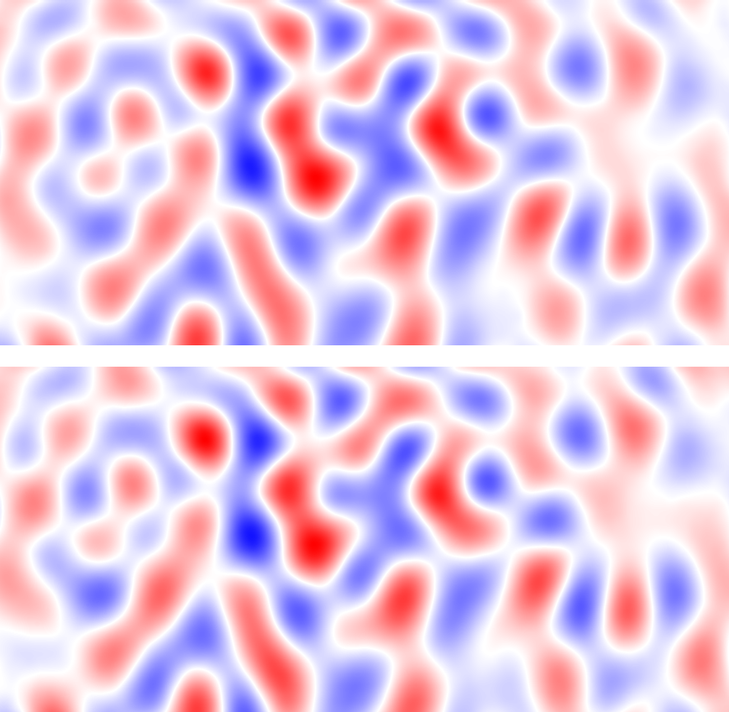
Figure 2: Correlation of BICEP2 (bottom) and Keck (top) E-mode polarization maps. The correlation coefficient $C=0.985$.

Fig. 1 shows the BICEP2 and Keck B-mode maps which we have digitized and plotted on a Mercator projection. The color scheme is one we used in Colley and Gott (2003). White is a B-mode of zero. Red ink indicates positive B-mode with the amount of red ink per pixel proportional to the value of the positive B-mode at that location. Blue ink indicates negative B-mode with the amount of blue ink per pixel proportional to the amount of negative B-mode at that location. In the figure, the maps are shown normalized in amplitude for easier comparison, but we measure $\sigma_{B}=0.0838\mu\mbox{K}$, and $\sigma_{K}=0.0673\mu\mbox{K}$ from the digitized maps. Importantly, the Keck map has a smaller amplitude, which means that according to Eqs. 5 and 6 that it has smaller noise. The two maps are not equally good. Secondly, since $C=0.566$ is surprisingly low (you can see that only about half the structures in the two maps agree) it means that the noise amplitudes, particularly for the BICEP2 map are surprisingly large. Solving Eqs. 5 and 6 we find:

$$\sigma_{BN}=0.0619\mu\mbox{K}=0.738\sigma_{B}$$ (7)

and

$$\sigma_{KN}=0.0366\mu\mbox{K}=0.544\sigma_{K}.$$ (8)

This implies values of

$$w=0.545$$ (9)

for BICEP2 (which is slightly more than twice the noise power that the BICEP2 paper claimed: i.e. that $w=0.24$), and

$$w^{\prime}=0.295$$ (10)

for Keck.

In other words, the Keck map has a value of $w^{\prime}$ which is similar to the value of $w$ originally claimed by BICEP2. Since the noise power in the BICEP2 map is much larger than we had supposed, by subtraction, the value of the power in gravitational waves must be consequently less. Note that these noise values are completely independent of the amount of dust signal. The noise levels in both maps can be estimated from the correlation coefficient and the amplitudes of the two maps, without reference to the dust.

We may check these noise estimates by using them to predict the correlation coefficient of the BICEP2 and Keck E-mode maps, which are of considerably higher amplitude. We will make the quite reasonable assumption that the noise levels in the two E-mode maps are the same as the noise levels we have just determined for the B-mode maps. The E-mode maps are shown in Fig. 2. They have been normalized for comparison, but the measured amplitudes of the two maps are:

$$\left(\sigma_{B}\right)_{E\textup{-modes}}=0.4497\mu\mbox{K},$$ (11)

and

$$\left(\sigma_{K}\right)_{E\textup{-modes}}=0.4341\mu\mbox{K}.$$ (12)

We can then plug in the values from Eqs. 7, 8, 11, 12 into Eq. 4 to determine two independent estimates of $C$. We can take the geometric mean of these two estimates to predict the value of $C$ between the two E-mode maps:

$$C_{\textup{predicted}} =\left[\left(\sigma_{B}^{2}-\sigma_{BN}^{2}\right)\left(\sigma_{K}^{2}-\sigma_{KN}^{2}\right)/\left(\sigma_{B}\sigma_{K}\right)^{2}\right]^{1/2}$$ (13)

$$=0.9869$$

Thus, the predicted correlation between the two E-mode maps should quite high. The observed correlation coefficient between the two E-mode maps is:

$$C_{\textup{observed}}=0.985$$ (14)

This is an extraordinary agreement. In our previous paper (Colley & Gott 2015) we showed that given the small number of modes (and structures) shown in the BICEP2 region, the accuracy of the correlation coefficient is ($\pm 0.04$ $[1\sigma]$). We showed this by measuring the correlation coefficient between the BICEP2 B-mode map and random fields, where the correlation should be zero. Thus our predicted value for the correlation coefficient of the E-mode maps is within $1\sigma$ of the observed value. Visual inspection of the two maps shows them to be virtually identical, with the same structures appearing at the same locations. This shows the telescopes are working as well as we claim. The B-mode maps show a lower correlation because they have a lower signal-to-noise ratio.

We may determine the $1\sigma$ errorbars on $w$ and $w^{\prime}$ (for BICEP2 and Keck) by repeating the calculations for deriving Eqs. 9 and 10 using $C=0.566\pm 0.04(1\sigma)$ in Eqs. 5 and 6. Thus, we find:

$$w=0.545\pm 0.033(1\sigma)$$ (15)

$$w^{\prime}=0.295\pm 0.050(1\sigma).$$

3 Correlation with Planck 353 GHz Map

As in our previous paper (Colley & Gott 2015), we use the publicly available Planck data at $353\mbox{GHz}$ (Stokes polarization parameters U and Q) to compute the B polarization modes. At this frequency polarized emission in the sky is surely dominated by dust polarization. We compare the $353\mbox{GHz}$ B-mode map with the BICEP2 B-mode map. If the two agree, with positive and negative (clockwise and counterclockwise swirls in polarization) regions at the same locations this would constitute a proof that the B-mode polarization was due to dust and not gravitational waves. It would falsify the claim that the particular B-modes seen in the BICEP2 map were due to gravitational waves. This makes no specific assumption about the amplitude of the dust polarization at $150\mbox{GHz}$, just that the dust is in the same locations and that the polarization angles are similar at the two frequencies. If all the features detected in the BICEP2 B-mode map are explained by features already found in the Planck dust B-mode map, the detection of gravitational waves would be falsified.

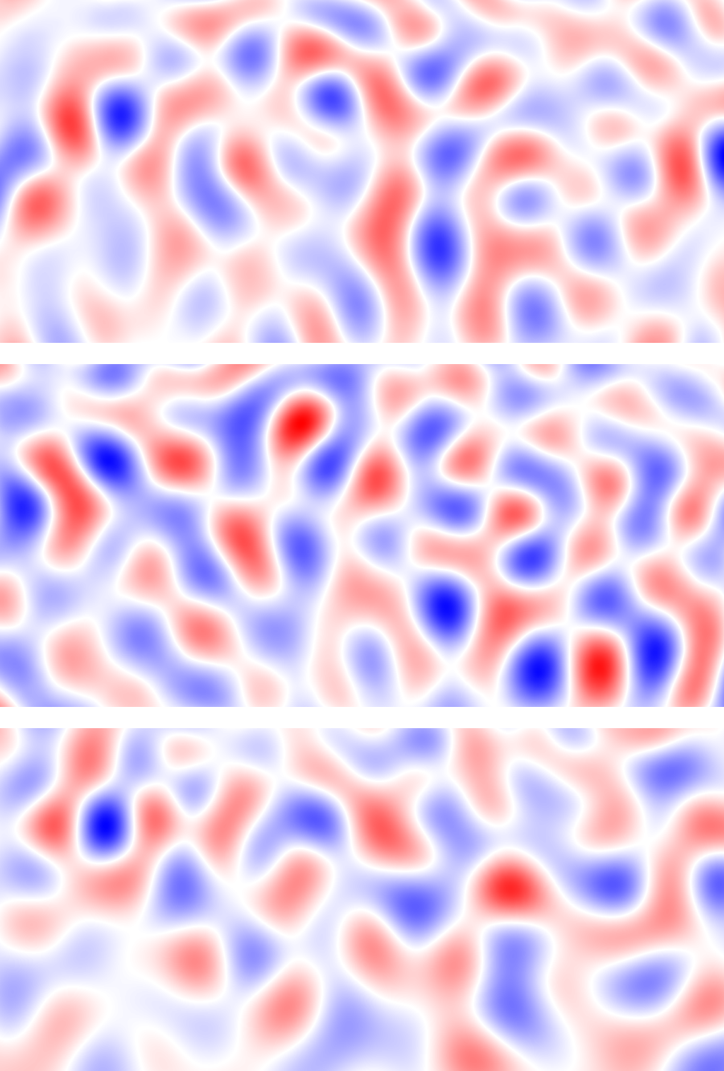
Figure 3: Keck (top) and BICEP2 (middle) B-modes compared with Planck 353 MHz dust polarization map (bottom).

The B-mode maps from Keck and BICEP2 compared with the dust polarization map from Planck are shown in Fig. 3. The Planck map we show in Fig. 3 is produced from the publicly available Planck U and Q maps we have digitized and from which computed the B polarization modes using spin 2 spherical harmonics. As in the Keck and BICEP2 maps, we show only Planck B-modes $(50<l<120)$ at $353\mbox{GHz}$ in the BICEP2 region. The BICEP2 team which also ran Keck also used a third degree polynomial spline fit on each half of each horizontal scan. Therefore we have applied exactly this spline fitting with third degree polynomials in each half of each horizontal scan to reproduce what was done in the Keck and BICEP2 maps. We have tapered the map in exactly the same way the BICEP2 map was tapered. This lowers confusion between E- and B-modes. In our previous paper this Planck map appeared as Map IV. Of the different mapping techniques, it produced the highest correlation coefficient between BICEP2 and the Planck $353\mbox{GHz}$ map. This was also the favored mapping technique (tapered map) used by the joint analysis by the Planck and BICEP2 + Keck teams.

The correlation coefficients are low:

Keck vs Planck: $$C=0.259$$ (16)

BICEP2 vs Planck: $$C=0.181$$

This shows that a dust signal is detected in both maps at greater than $4\sigma$, since the uncertainty in the correlation coefficient at $1\sigma$ is 0.04. Since the correlation coefficient is low in both cases, this suggests that dust is not the dominant signal in the maps. It also suggests that Keck is a better (lower noise) map than BICEP2 because it sees a higher correlation coefficient with the dust map, a signal which both are detecting. This agrees with the fact that we have deduced already that the noise in the Keck map is lower than in the BICEP2 map. We may use the correlation coefficients to estimate the amplitude of the dust signal.

We have developed formulas for this from our previous paper (Colley & Gott 2015). Previous studies have considered only the power spectrum of the B-modes. But they leave out the other information in the maps. We are only making use of the publicly available BICEP2 data and Planck data that were already utilized by the BICEP2 team and Flauger, Hill & Spergel (2014). We are just using them in a different, and complementary way to directly look at the B-mode maps and their correlations.

One supposes the BICEP2 team wanted to show a map that would show just the modes where the gravitational wave modes were most prominent. The BICEP2 team filtered out the high-$l$ modes to avoid confusion with the B-modes from gravitational lensing, and presumably filtered out the low-$l$ modes to avoid confusion with dust. This is because the power spectrum in the dust B-modes is very flat. For dust $\Delta_{BB}^{2}=l(l+1)C_{l}/2\pi\sim l^{-0.4}$. The flat nature of the power spectrum for the dust is shown in Flauger, Hill & Spergel (2014). On the other hand, for the B-modes expected from gravitational waves (and gravitational lensing) $C_{l}\sim\mbox{const}$, so that $\Delta_{BB}^{2}=l(l+1)C_{l}/2\pi\sim l^{2}$ over the range $10<l<80$. (For $l>100$ the gravitational wave B-mode spectrum begins to fall and crosses below the gravitational lensing power at $l\approx 150$.)

The BICEP2 team also included a simulation with B-modes produced by gravitational lensing only. The power spectrum from gravitational lensing over the range $10<l<100$ also has $C_{l}\sim\mbox{const}$, so that $\Delta_{BB}^{2}=l(l+1)C_{l}/2\pi\sim l^{2}$. Noise power (Poisson noise) is expected to be similar, with $C_{l}\sim\mbox{const}$, and that $\Delta_{BB}^{2}=l(l+1)C_{l}/2\pi\sim l^{2}$. In our previous paper (Colley & Gott 2015), using the previously published Planck estimate that the polarized dust emission $I_{\nu}\sim\nu^{3+\beta}/[\exp(h\nu/kT_{D})-1]$, where $\beta=1.65$, and $T_{D}=19.8K$ for high latitude dust, we found that the amplitude of fluctuations in brightness temperature in the polarized dust at $150\mbox{GHz}$ should be lower than the amplitude at $353\mbox{GHz}$ by a factor of 21.3. Later, the joint analysis by the Planck and Keck + BICEP2 teams found this factor to be approximately 25. We shall adopt that factor of 25 here.

The rms amplitude of the spline-fitted $50<l<120$ B-mode map is $\sigma_{353}=2.96\mu\mbox{K}$. If we lower this by a factor of 25 we will get an amplitude of $\sigma=0.118\mu\mbox{K}$ which is larger than the similarly filtered BICEP2 B-mode map rms amplitude of $\sigma_{B}=0.0838\mu\mbox{K}$. The discrepancy is resolved by the fact that the Planck B-mode map contains noise (instrument noise plus any systematic effects) as well as the polarized dust emission signal. We may directly determine the amplitude of the polarized dust signal at $150\mbox{GHz}$ from the observed correlation coefficient between the BICEP2 map and the Planck map at $353\mbox{GHz}$.

We do find a correlation coefficient of $C=0.181$ between the filtered BICEP2 map and the similarly filtered $353\mbox{GHz}$ map from Planck (whose signal is dominated by polarized dust). This shows the dust is peeking through in both maps (the correlation is positive). To test if this 18.1% correlation could be due to noise only we cross-correlated the BICEP2 map with 7 random $353\mbox{GHz}$ maps by flipping and mirror imaging Planck regions, the rms correlation (or anti-correlation) with the 7 random maps was $\sigma=4.0\%$. Thus, the observed correlation is $18.1\%\pm 4.0\%$ ($1\sigma$), significant at $4\sigma$.

Now we will analyze the situation in detail. The BICEP2 map and the Planck $353\mbox{GHz}$ map have a correlation coefficient of 18.1%. The BICEP2 spline-fitted map in the $50<l<120$ modes has a $1\sigma$ amplitude of $\sigma_{B}=0.0838\mu\mbox{K}$ while the Planck $353\mbox{GHz}$ spline-fitted map in the $50<l<120$ modes has a $1\sigma$ amplitude of $\sigma_{353}=2.96\mu\mbox{K}$. Thus, $\sigma_{353}=35.3\sigma_{B}$. Now

$$\sigma_{B}^{2}=\sigma_{BGW}^{2}+\sigma_{BD}^{2}+\sigma_{BGL}^{2}+\sigma_{BN}^{2},$$ (17)

where $\sigma_{BGW}$ is the standard deviation of the BICEP2 gravitational wave signal, $\sigma_{BN}$ is the standard deviation of the BICEP2 noise, $\sigma_{BGL}$ is the standard deviation of BICEP2 gravitational lensing signal, and $\sigma_{BD}$ is the standard deviation of the BICEP2 dust signal (since all these are uncorrelated with each other). With $x$, $y$, $z$ and $w$ as defined earlier:

$$\sigma_{B}^{2}=(x+y+z+w)\sigma_{B}^{2}.$$ (18)

The BICEP2 team produced a simulation showing only the expected gravitational lensing and noise. From their graph of the simulated gravitational lensing power spectrum we deduced $z=\sigma_{BGL}^{2}/\sigma_{B}^{2}=0.1955$. This corresponds to a standard $A_{L}=1$ power in lensing expected from the standard flat-lambda model. In this paper we have determined that $\sigma_{BN}^{2}/\sigma_{B}^{2}=w=0.545$ (Eq. 9).

Since $x+y+z+w=1$, we find:

$$x+y=0.2595.$$ (19)

The amplitude of the gravitational waves, and gravitational lensing B-mode signals are independent of frequency, so the amplitude of those signals, $\sigma_{BGW}$ and $\sigma_{BGL}$, are equal in the two maps.

Using this, we will now substitute in the formula for the correlation coefficient between the BICEP2 and Planck $353\mbox{GHz}$ map, to obtain:

$$C=18.1\%\\ =(\sigma_{BGW}^{2}/\sigma_{B}\sigma_{353})+(\sigma_{BD}\sigma_{353}/\sigma_{B}\sigma_{353})+\\ (\sigma_{BGL}^{2}/\sigma_{B}\sigma_{353}).$$ (20)

Since $\sigma_{B}=0.0838\mu\mbox{K}$ and $\sigma_{353}=2.96\mu\mbox{K}$, $\sigma_{353}=35.3\sigma_{B}$. We know $w=\sigma_{BN}^{2}/\sigma_{B}^{2}=0.545$. Also we know $\sigma_{353D}=25\sigma_{BD}$. Substituting, we get:

$$C=18.1\%\\ =(\sigma_{BGW}^{2}/35.3\sigma_{B}^{2})+(25\sigma_{BD}^{2}/35.3\sigma_{B}^{2})+\\ (\sigma_{BGL}^{2}/35.3\sigma_{B}^{2})$$ (21)

$$6.39=(\sigma_{BGW}^{2}/\sigma_{B}^{2})+(25\sigma_{BD}^{2}/\sigma_{B}^{2})+(\sigma_{BGL}^{2}/\sigma_{B}^{2}).$$ (22)

We know $z=\sigma_{BGL}^{2}/\sigma_{B}^{2}=0.1955$, so

$$6.39 =x+25y+0.1955$$ (23)

$$6.19 =x+25y.$$

Substituting from Eq. 19 ($x+y=0.2595$, or $x=0.2595-y$) for $x$ we find:

$$5.93=24y$$ (24)

$$y=0.247$$

$$x=0.0125.$$

The $1\sigma$ uncertainty in $C$ is $\pm 4.0\%$ so we can repeat the steps from Eq. 22 on with $C$ equal to 22.1% and 14.1% to obtain the limits:

$$y=0.247\pm 0.06(1\sigma)\\$$ (25)

Now the value of $z=0.1955$ has been estimated from lensing simulations assuming a standard flat-$\Lambda$ model. Such simulations for a sample this size show a standard-deviation of $\pm 50\%$. Thus we find that $z=0.1955\pm 0.09775(1\sigma)$. From previous results, we know that $w=0.545\pm 0.033(1\sigma)$ and $y=0.247\pm 0.06(1\sigma)$. The errors in $z$, $w$ and $y$ should be uncorrelated. Since $1=x+y+z+w$ and $x$ is deduced by subtraction, the errors in $z$, $w$ and $y$ should add in quadrature to give the ($1\sigma$) error in $x$:

$$\sigma_{x}^{2}=0.09775^{2}+0.033^{2}+0.06^{2}=0.119^{2};$$ (26)

thus,

$$x=0.0125\pm 0.119(1\sigma).$$ (27)

BICEP2 estimated the ratio $r$ of power in tensor-to-scalar modes to be $r=0.20$ assuming that $y=0$ and fitting the excess power they observed over and above their simulation including gravitational lensing and noise. That was equivalent to a value of $x=0.565$ using their assumed noise. Thus $r$, being proportional to $\sigma_{BGW}^{2}$, is related to $x$ by $r=0.2(x/0.565)$ which we will use to convert $x$ (in Eq. 27) to $r$ (in Eq. 28 below). They then estimated a realistic dust contamination could lower $r$ to 0.16, (corresponding to $x=0.452$ and $y=0.113$). This was close to Linde’s chaotic inflation prediction of $r=0.13$. In our previous paper (Colley & Gott 2015) we got $x=0.274$, and $r=0.099$ by getting a better (higher) estimate of the dust contamination $y=0.278$ using our correlation technique rather than the rough estimate BICEP2 made, raised a bit by using the factor of 21.3 (rather than 25), but, importantly, adopting the noise estimate from the BICEP2 paper. Now that we can measure the noise in BICEP2 directly from its correlation with Keck, we find that the value of $y$ is about the same as before $y=0.247\pm 0.06$, but the contribution from power in gravitational waves now vanishes:

$$r=0.004\pm 0.04(1\sigma)$$ (28)

$$\sigma_{BD}=0.042\mu\mbox{K}$$ (29)

What this means is that the power in the dust, gravitational lensing and noise, add together to completely explain the observed power in the B-modes (i.e. $\sigma_{B}^{2}$) without any need for gravitational waves ($x$ is near zero to well within $1\sigma$). Thus, there is no evidence for gravitational waves from the BICEP2 map.

We can repeat this analysis for Keck versus Planck.

$$C=25.9\%\\ =(\sigma_{KGW}^{2}/\sigma_{K}\sigma_{353})+(\sigma_{KD}\sigma_{353D}/\sigma_{K}\sigma_{353})+\\ (\sigma_{KGL}^{2}/\sigma_{K}\sigma_{353}).$$ (30)

Since $\sigma_{K}=0.0673\mu\mbox{K}$ and $\sigma_{353}=2.96\mu\mbox{K}$, $\sigma_{353}=44.0\sigma_{K}$. We know $w^{\prime}=\sigma_{KN}^{2}/\sigma_{K}^{2}=0.295$. Also we know that $\sigma_{353D}=25\sigma_{KD}$. Substituting, we get:

$$C=25.9\%\\ =(\sigma_{KGW}^{2}/44.0\sigma_{K}^{2})+(25\sigma_{KD}^{2}/44.0\sigma_{K}^{2})+\\ (\sigma_{KGL}^{2}/44.0\sigma_{K}^{2})$$ (31)

$$11.40=(\sigma_{KGW}^{2}/\sigma_{K}^{2})+(25\sigma_{KD}^{2}/\sigma_{K}^{2})+(\sigma_{KGL}^{2}/\sigma_{K}^{2}).$$ (32)

We know $z^{\prime}=\sigma_{KGL}^{2}/\sigma_{K}^{2}=0.1955\sigma_{B}^{2}/\sigma_{K}^{2}=0.2966$, so

$$11.40 =x^{\prime}+25y^{\prime}+0.2966$$ (33)

$$11.10 =x^{\prime}+25y^{\prime}.$$

Since $x^{\prime}+y^{\prime}=0.4074$, or $x^{\prime}=0.4074-y^{\prime}$ for $y^{\prime}$ and $x^{\prime}$ we find:

$$10.69 =24y^{\prime}$$ (34)

$$y^{\prime} =0.4455$$

$$x^{\prime} =-0.0381.$$

The $1\sigma$ uncertainty in $C$ is $\pm 4.0\%$ so we can repeat the steps from Eq. 29 on with $C$ equal to 21.9% and 29.9% to obtain the limits:

$$y^{\prime}=0.4455\pm 0.07(1\sigma).$$ (35)

Repeating steps leading to Eq. 27, we find:

$$\sigma_{x^{\prime}}^{2}=0.1483^{2}+0.050^{2}+0.07^{2}=0.171^{2};$$ (36)

thus,

$$x^{\prime}=-0.0381\pm 0.171(1\sigma).$$ (37)

For Keck, $r$, being proportional to $\sigma_{KGW}^{2}$, is related to $x^{\prime}$ by $r=0.2(x^{\prime}[\sigma_{K}^{2}/\sigma_{B}^{2}]/0.565)$ which we will use to convert $x^{\prime}$ (from Eq. 37) to $r$ (in Eq. 39 below).

$$r^{\prime}=-0.0087\pm 0.039(1\sigma),$$ (38)

or, keeping only significant figures,

$$r^{\prime}=-0.01\pm 0.04(1\sigma).$$ (39)

$$\sigma_{KD}=0.045\mu\mbox{K}.$$ (40)

What this means, again, is that the power in the dust, gravitational lensing and noise, add together to completely explain the observed power in the B-modes (i.e. $\sigma_{B}^{2}$) without any need for gravitational waves (i.e. no need for $x>0$). Of course a negative value of $x$ is unphysical, but we notice that $x$ is within $1\sigma$ of zero. The maximum likelihood value of $x$ is zero, thus there is no evidence for gravitational waves from the Keck map.

Note, that the two estimates of $\sigma_{BD}$ and $\sigma_{KD}$ agree to within about 9%, which is reassuringly close.

Median statistics (Gott et al. 2001) tell us that we have two independent estimates of $r$, and if there are no systematic effects, there is a 50% chance that the true value of $r$ lies between -0.0087 and +0.004. Thus Starobinsky (1982) inflation which has a value of $r$ = 0.0036 [smaller than that of Linde (1983) chaotic inflation ($r$ = 0.13) by a factor of 36] is not ruled out. Starobinsky inflation also predicts the correct value of $n_{s}$ (the tip in the inflationary power spectrum). All these variables are approximately Gaussian distributed because we have shown that these maps are all approximately Gaussian random fields in the modes shown (Colley & Gott 2015). Thus, given just these two measurements of $r=0.004$ and $r=-0.0087$, the probability distribution of $r$ values can be estimated using the Student’s $t$ distribution with $n=2$, which is a Cauchy distribution. The probability of the true value of $r$ being as large or larger than 0.0036 is 26%. So Starobinsky inflation is not ruled out. The probability of the true value of $r$ being as large or larger than 0.13 is 1.5%. So Linde chaotic inflation is excluded at the 98.5% confidence level even under the very conservative hypothesis that we have no systematic effects and only going on the two values we have obtained. The Cauchy distribution has very broad wings, and even so, the value of 0.13 is excluded. Stronger limits can be derived if one puts in the probable limits we have on other parameters such as the correlation coefficients, with tests against random fields. That gives the stronger limits quoted in Eqs. 28 and 39.

4 Independent Estimation of the Gravitational Lensing Signal

For the Keck sample, which is the more accurate, we find $z^{\prime}=0.2966$ from simulations, following a procedure similar to that used by the BICEP2 team. This should be accurate to $\pm 50\%$ given the size of the sample on the sky. This estimate is from computer simulations of the standard cold dark matter $\Lambda\mbox{CDM}$ cosmological model. Another approach is to attempt to calculate it directly by deducing the lensing potential from shear in the CMB temperature map and using this potential on the E-modes seen in the CMB (with dust subtracted) to produce a B-mode map. This has now been done by the Planck team (Planck Collaboration 2016). They have produced a “Commander” map of the temperature map of the CMB. This has had dust subtracted out as best as possible. So it is a map of the temperature fluctuations coming directly to us directly from the CMB. Shear can be measured from this map, and a map of the cold dark matter potential can be made from this. Gradients of this potential will show displacement of pixels from their original map positions due to gravitational lensing by cold dark matter. Inflation should produce pure E-modes, if there were no gravitational radiation from the early universe. But displacements of the pixels by gravitational lensing would generate B-mode patterns of small magnitude from the observed E-modes. Knowing the map of the E-modes, one can make a map of the B-modes produced by the gravitational lensing (deduced from the shear measurements). The Planck team has made such a B-mode map from gravitational lensing alone. We have compared this B-mode map from Planck due to lensing alone with the Keck B-mode map in Fig. 4.

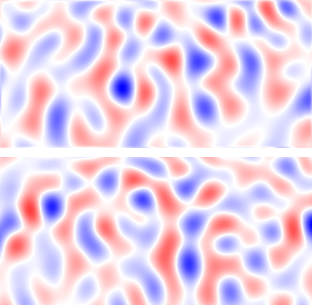
Figure 4: Planck lensing B-modes (top) compared with Keck B-modes (bottom).

The correlation coefficient between these two maps is surprisingly small $C=0.11$—significant, but very small. We then compared the E-mode map from the Commander map with the Keck E-mode map (see Fig. 5).

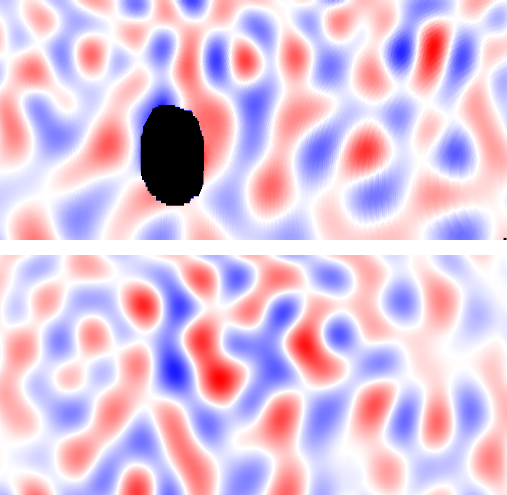
Figure 5: Planck E-modes (top) compared with Keck E-modes (bottom). The black region is excised due to an artifact in the Planck data.

The correlation was only $C=0.26$. We know the Keck E-mode map has a high signal-to-noise because it has a correlation coefficient of $C=0.985$ with the BICEP2 map, so the small correlation must be due to the larger noise in the E-mode Planck Commander map, coupled with the fact that the Keck E-mode map has some small dust component. It is known from Planck that the amplitudes of the E and B-modes in the dust polarization are approximately equal. For Keck, $(\sigma_{K})_{E\textup{-modes}}=0.4341\mu\mbox{K}$, while $(\sigma_{K})_{B\textup{-modes}}=0.0673$. The fraction of the B-mode power in the dust is $y^{\prime}=0.4455$. Thus $(\sigma_{K})_{B\textup{-modes,dust}}=0.0673\mu\mbox{K}(0.4455)^{1/2}=0.0449\mu\mbox{K}$. Planck results that E- and B-modes in dust polarization are approximately equal indicate that $(\sigma_{K})_{E\textup{-modes,dust}}\approx(\sigma_{K})_{B\textup{-modes,dust}}=0.449\mu\mbox{K}$.

Thus, the power in E-modes from dust relative to the total E-mode power in the Keck data is approximately $[(\sigma_{K})_{E\textup{-modes,dust}}]^{2}/[(\sigma_{K})_{E\textup{-modes}}]^{2}\approx(0.0449\mu\mbox{K})^{2}/(0.4341\mu\mbox{K})^{2}\approx 0.01$, or insignificant. Thus, we expect the E-mode Keck map not to be significantly corrupted by dust, and as such, it can be directly compared to the Planck Commander E-mode map. As we have said their correlation coefficient is low $C=0.26$. This must be due primarily to noise in the Planck map since, the noise power in the Keck E-mode map is approximately $w^{\prime\prime}\approx w^{\prime}[(\sigma_{K})_{B\textup{-modes}}]^{2}/[(\sigma_{K})_{E\textup{-modes}}]^{2}\approx 0.296(0.0673\mu\mbox{K})^{2}/(0.4341\mu\mbox{K})^{2}\approx 0.01$, again negligible. Errors in the E-mode map are due in part from the fact that in the Commander map a small region within the Keck sample has been excised. When the E-mode map is made we must taper the map in this region and this causes an additional error in the E-modes. We therefore taper the Keck map in the same way and excise the same region when computing the correlation coefficient of $C=0.26$. Still, this excised region is unfortunate.

Now if the correlation coefficient of the Planck and Keck E-mode maps is $C=0.26$ then the E-mode map from which the lensing potential gradients are producing the B-mode map is mostly wrong, see Fig. 5. Even if the potential gradients were calculated perfectly and the B-mode signal in the Keck map were actually due entirely to gravitational lensing, we might expect the correlation between the Keck B-mode map and the Planck B-mode lensing map to be only $C=0.26$. The B-mode lensing map can only be as good as the Commander E-mode map it is derived from. Actually the Planck B-mode lensing map has an even lower correlation coefficient with the Keck B-mode map: $C=0.11$. Thus, we may roughly estimate that the fraction of the B-mode power in the Keck map due to gravitational lensing is $z^{\prime}\sim 0.11/0.26=0.42$. This compares well with the estimate of $z^{\prime}=0.2966\pm 0.1483$ for Keck, calculated from cold dark matter simulations which we have used in the above sections. In other words, this independent analysis of the power in the gravitational lensing produced B-modes is consistent with the power assumed earlier from from the computer cold dark matter simulations. There is no evidence that the gravitational lensing in this region is particularly low, for example.

A couple of points should be mentioned. First of all the $B_{l}$ mode amplitudes produced by gravitational lensing are weighted sums of terms like $E_{l^{\prime}}K_{l^{\prime\prime}}$ where $l^{\prime}+l^{\prime\prime}=l$ and $K$ is the gravitational potential. Thus the $B_{l}$ modes we are showing in our map $(50<l<120)$ depend on modes $(2<l<120)$ in the E-modes and in the gravitational potential ($K$) modes. The Planck data does include these lower E- and K-modes. Our E-mode map does not include modes below $l=50$. Our E-mode map filtered to show only $(50<l<120)$ is directly comparable with their E-mode map which we have filtered in exactly the same way. And our B-mode map filtered to show only $(50<l<120)$ is directly comparable with their B-mode lensing map which we have shown filtered the same way. But we could not simply take their gravitational potential map and apply it to our E-mode map to produce an improved B-mode lensing map because we would be missing the E-modes with $l^{\prime}<50$ which would be needed to calculate the B-modes between 50 and 120. But it is clear that the E-modes they are using in the range 50 – 120 are not as accurate as the ones we have. If we hope in future experiments to push toward values of lower $r$ such as $r=0.03$ or even lower, comparable with Starobinsky’s inflationary estimate of $r=0.0036$, we must deal accurately with the gravitational lensing background. The Planck technique offers a way to produce a map of the gravitational lensing background in B-modes, which could be subtracted from the data, just as we can subtract the dust signal, but it would have to be done at much higher signal to noise, to push to significantly lower levels of $r$. Large area surveys are currently underway with SPIDER in Antarctica which promise to survey regions of lower dust contamination and have higher accuracy. We could likewise look within low dust regions for those that happen to have lower lensing (perhaps by 50%) as well. The cold dark matter gravitational potential map Planck produces is ideal in that it integrates all the way back to the cosmic microwave background, which is exactly what is needed. But this can be supplemented and checked by gravitational potential tomography maps obtained from lensing shear deduced from background galaxies in deep surveys.

We have checked our maps to see if any two-sigma peaks or valleys in the B-mode Keck map can be seen as two-sigma peaks or valleys in the B-mode dust maps or the B-mode lensing maps. See Fig. 6. If these were uncorrelated, one would expect the $(\text{coincidences}-\text{anti-coincidences})$ in peaks and valleys to be zero on average. We find 5 coincidences between the Keck dust maps, and $(2\text{~{}coincidences}-1\text{~{}anti-coincidence})=1$ between the Keck and lensing maps, consistent with the expectation that the dust signal is expected to be stronger than the lensing signal, and the lensing map is more inaccurate. The dust and lensing maps show only $1\text{~{}anti-coincidence}$, consistent with the fact that we expect them to be uncorrelated.

Figure 6: Overlap of $2\sigma$ departures in Keck B-modes (high red, low blue), Planck lensing B-modes (high magenta, low green) and Planck 353GHz dust B-modes (high orange, low cyan).

5 Future Prospects—Primordial Gravitational Radiation = Hawking Radiation

In the standard calculation of the gravitational radiation in the early Universe (for example Maldacena & Pimentel [2011]), in calculating the graviton propagator one uses the Bunch-Davies vacuum (Bunch & Davies 1978), which is equivalent the Gibbons and Hawking thermal vacuum (Gibbons & Hawking 1977), which includes Gibbons and Hawking thermal radiation (Gibbons & Hawking 1977), which is Hawking radiation (Hawking 1974) from the causal horizon in the early Universe. If such gravitational radiation were found, it would constitute a confirmation of the Hawking (1974) mechanism. This gravitational radiation is produced by a quantum process quite different from the gravitational waves recently discovered by LIGO (e.g. LIGO and Virgo Collaborations 2016), which is in the classical gravitational wave domain.

The possibility that Hawking radiation from the inflationary epoch could be observed today was mentioned in a different context by Gott (1982), who proposed the formation of bubble universes by quantum tunnelling during inflation producing what we would call today a multiverse. The CMB is thermal radiation left over from the earliest times. Inflation produces causal horizons which produce Gibbons and Hawking (1977) radiation through the Hawking (1974) radiation process. Gott (1982) speculated in this case that if inflation began at the Planck density, the CMB radiation we see today might be the thermal radiation generated by the causal horizons in the early universe by inflation. In hindsight, a trouble with this mechanism we would note today is that it would produce fluctuations in the CMB of order unity (since inflation would occur at the Planck scale) whereas we observe fluctuations of order $10^{-5}$ in the CMB, suggesting that the end of Inflation occurs at significantly sub-Plankian energy scales.

However, Hawking radiation includes gravitational radiation as well as electromagnetic radiation (Page 1976). We may calculate the magnitude of the energy density of this gravitational radiation during the inflationary phase from a back of the envelope calculation using the causal horizons. If the expansion is exponential with $a(t)$ proportional to $\exp(t/r_{0})$, then the radius of the de Sitter space approximating spacetime at that epoch is $r_{0}$. The Hubble constant during inflation is $H=1/r_{0}$. The Gibbons and Hawking thermal temperature is $T=1/2\pi r_{0}$. Ignoring constants of order unity, the energy density of the Gibbons and Hawking gravitational radiation is of order $T^{4}\sim 1/r_{0}^{4}$.

Let us make the order of magnitude calculation a different way using the uncertainty principle. The causal horizon is at a proper distance of $r_{0}\pi/2$ and the circumference of the causal horizon is $2\pi r_{0}$. The causal volume inside the causal horizon of the observer is $\pi^{2}r_{0}^{3}$. The energy density of gravitational radiation is (Misner, Thorne & Wheeler 1973):

$$T_{00}^{GR}=(1/32\pi)\omega^{2}(|A_{+}|^{2}+|A_{\times}|^{2}),$$ (41)

where $\omega$ is the angular frequency, and $A_{+}$ and $A_{\times}$ are the amplitudes of the two polarization states. From the uncertainty principle we expect on a scale of $L$ to find (Misner, Thorne & Wheeler 1973) uncertainties in the metric: $\Delta g\sim(L_{p}/L)$ where $L_{p}$ is the Planck Length. Since we are using Planck units here, $L_{p}=1$ and:

$$\Delta g\sim(1/L)\sim 1/r_{0}$$ (42)

since one can only see out to the causal horizon. Likewise the wavelengths of the waves you are seeing must also be $\sim L$, so their frequency $\nu\sim(1/L)$.

Thus: $\omega=2\pi\nu$, and

$$(1/32\pi)\omega^{2}\sim(1/L)^{2}\sim(1/r_{0})^{2}.$$ (43)

Now the amplitude of the waves $A$ is $\Delta g$ so:

$$(|A_{+}|^{2}+|A_{\times}|^{2})\sim(\Delta g)^{2}\sim(1/r_{0})^{2}.$$ (44)

So substituting these two results in the equation $T_{00}^{GR}=(1/32\pi)\omega^{2}(|A_{+}|^{2}+|A_{\times}|^{2})$ found above, we find of order

$$T_{00}^{GR}\sim(1/r_{0})^{4},$$ (45)

in agreement with the value found earlier for gravitational Gibbons and Hawking radiation at the Hawking temperature from the causal horizons. (By the way, the energy of a typical graviton in this radiation is $E_{\text{graviton}}\sim h\nu\sim kT\sim 1/2\pi r_{0}$). The total energy inside the causal horizon volume is $\sim(\pi/8r_{0}^{4})(\pi^{2}r_{0}^{3})\sim\pi/r_{0}$. Dividing by the energy of a typical graviton gives $\sim 2\pi^{2}$ gravitons within the causal horizon.) These gravitational waves have an amplitude $(\Delta g)\sim(1/r_{0})$ as they redshift out of the causal horizon. When Inflation ends, and the universe begins to decelerate, these will eventually come back inside the causal horizon with also an amplitude of order $(\Delta g)\sim(1/r_{0})$ (Bardeen, Steinhardt & Turner 1983). This means that in terms of the power spectrum, the power in fluctuations due to gravitational radiation is proportional to the amplitude of the waves squared: $(\Delta g)^{2}\sim(1/r_{0})^{2}\sim H^{2}$ during inflation, where we are using Planck units. Maldacena & Pimentel (2011) note in their Eq. 2.20 that the gravitational wave expectation values have the following order of magnitude: $\langle\gamma\gamma\rangle\sim H^{2}/M_{pl}^{2}$, or, in Planck units: $\langle\gamma\gamma\rangle\sim H^{2}$ in agreement with what we have stated above. Krauss and Wilczek (2014) have similarly noted the gravitational waves display a dimensionless power spectrum at the horizon, given by:

$$\Delta^{2}(k)=(k^{3}/2\pi^{2})P_{t}=(2/\pi^{2})H^{2}/M_{pl}^{2}$$ (46)

and they have correctly noted that detection of the primordial B polarization modes would constitute empirical evidence for the quantization of gravity. They note the above relation means that the energy scale of inflation is

$$\epsilon_{\text{inflation}}=1.06\times 10^{16}\text{Gev}(r/0.01)^{1/4}=V^{1/4}.$$ (47)

Krauss and Wilczek also say that detection of these primordial B polarization modes would constitute a detection of gravitons, since these waves are produced by production of individual gravitons by a quantum process. We are simply noting that the quantum process by which they are being created is just the Gibbons and Hawking process or the Hawking radiation mechanism, and that detection of the primordial gravitational radiation through their B polarization modes would also constitute a detection of Hawking radiation as well (this time coming from microscopic cosmological causal horizons, thus making them observable). By contrast, macroscopic black hole horizons (i.e. $>6~{}\text{km}$) produce Hawking radiation below detectable limits. This connection to proving Hawking radiation further raises the scientific stakes for a successful detection of primordial B-mode polarization.

References

- BardeenSteinhardtTurner (1983) Bardeen, J.M, Steinhardt, P.J. & Turner, M.S., 1983, PhysRevD, 28, 679
- BunchDavies (1978) Bunch, T.S. & Davies, P.C.W., 1978, Journal of Physics A, 11, 1315
- BICEP2 (2014) BICEP2 Collaboration, 2014, PhysRevLett, 112, 241101
- ColleyGott (2003) Colley, W.N. & Gott, J.R., 2003, MNRAS, 344, 686
- ColleyGott (2015) Colley, W.N. & Gott, J.R., 2015, MNRAS, 447, 2034
- FlaugerEtAl (2014) Flauger, R., Hill, J.C. & Spergel, D.N., 2014, Journ of Cosmology and Astroparticle Physics, 8, 039
- GibbonsHawking (1977) Gibbons, G.W. & Hawking, S.W., 1977, PhysRevD, 15, 2752
- Gott (1982) Gott, J.R., 1982, Nature, 295, 304
- Gott (1989) Gott, J.R, et al., 1989 ApJ, 340: 625
- GottEtAl2001 (2001) Gott, J.R, Vogeley, M.S., Podariu, S. & Ratra, B., 2001, ApJ, 549: 1
- KraussWilczek (2014) Krauss, L.M. & Wilczek, F., 2014, arXiv: 1309.5343v2 [HEPTH]
- LIGOVirgo (2016) LIGO Scientific Collaboration and Virgo Collaboration, 2016, PhysRevLett 116, 061102
- Linde (1983) Linde, A.D., 1983, Phys Lett B, 129, 3-4, 177
- MaldacenaPimentel (2011) Maldacena, J. & Pimentel, G.L., 2011, Journal of High Energy Physics, article id. 45
- (15) Misner, C.W., Thorne, K.S. & Wheeler, J.A., 1973, Gravitation, Freeman, San Francisco
- MortonsonSeljak (2015) Mortonson, M. J. & Seljak, U., 2015, PhysRevD, 92, 123507
- Page (1976) Page, D.N., 1976, PhysRevD, 14, 3260
- PlanckBLensMap (2016) Planck Collaboration, 2016, A&A, 596, 102
- Starobinsky (1983) Starobinsky, A.A., 1982, Physics Letters B, 117, 175