Optimal separation between vehicles for maximum flow through a light signal.

Abstract

The traffic flow through a light signal is explored by using the optimal velocity model and its improvement known as full velocity differences model. The simulations consider a single line of identical cars, equally spaced, and with no obstacles after the signal crossing line. The flow dependence on vehicle’s characteristics, as it’s length and sensitivity, are studied. Also, the influence of the attitude of drivers (careful or aggressive) has been used as parameters on the present work. It was found that the optimal separation between cars, defined as the distance that allows the system to carry the higher number of vehicles through the signal crossing line, is independent of the sensitivity of the system, but it does depend on the aggressive or careful characteristic of the drivers. The optimal separation is also found to be proportional to the length of the cars for a system of identical vehicles.

1 Introduction

Traveling by car or another vehicle is a part of daily life for modern human beings. And the amount of cars running over the streets is increasing fast thanks to the mass production and the lowering on the buying cost. Then the free flow over the streets is getting more difficult each day and it became apparent the necessity of finding ways to control and optimize such flow. Then, understanding how the traffic flow behaves is an important matter at present days, and because of that, it has been the focus of intensive research. For several decades the main object under investigation has been the formulation of an appropriated model to describe the most of the relevant observable phenomena [1, 2, 3, 4, 5, 6, 7, 8, 9]. Many models has been proposed and characterized during the last few decades, as can be revisited in an historical overview of the proposed models found in [10]. Some of them are macroscopic, based on the theory of fluid mechanics; some others are microscopic, taken into account every vehicle and its interaction with the others.

Microscopic models, specially car following models are of interest due that they can simulate traffic flow using rules based on human behavior (a recent review on those can be found in [11]). Once an acceptable model has been built, it can be used to study some of the many possibles scenarios that a multi-particle problem can lead to. However, on the available scientific literature, most works deals with the formulation of models and there was not much work on its application to an specific problem. Only recently, some of the latest works has been addressed in that direction: examples of such are the effect of signal on the stability of under saturated flow [12]; control by to kind of periodic signals [13]; the green wave break down [14, 15, 16], and recently the analysis of the trip cost on a corridor with two entrance and one exit [17].

In this paper, the problem of finding the optimal distance between consecutive cars in a line, in front of a light signal, is addressed under the light of the optimal velocity (OV) and full velocity differences optimal velocity (FVDOV) models. Those models are proven to successfully reproduce the main features of real traffic flow [1, 6]. The optimal separation between cars is defined as the distance that allow the maximum flow through the signal crossing line, during the green time. To the best of this author knowledge, this problem has not been studied anywhere.

2 The optimal velocity model.

The optimal velocity model was first introduced by Bando and collaborators [1, 6] to model and study the dynamical behavior of the traffic flow. The Bando model consist in a one dimensional loop road of length $L$, filled with $N$ identical cars. The $n$th driver adjust its car velocity in terms of its headway (free way ahead), so he can safely drive as fast as possible while avoiding collisions. If the headway is small, the velocity must be small (safe velocity), but if the headway is large, the velocity could be adjusted up to get to the maximum velocity available or desirable. The dynamical equations are written as:

$$\dot{x}_{n} =v,$$ (1)

$$\dot{v}_{n} =a\left(f(\Delta x_{n})-v_{n}\right).$$ (2)

Where the position of the $n$th car is $x_{n}$, the preceding car’s position is $x_{n+1}$ and the headway is $\Delta x_{n}=x_{n+1}-x_{n}$. $a$ is called the sensitivity parameter, and its value determines how the vehicle react to a given impulse. The function $f$ is the optimal velocity (OV) function, which is set to be a continuous, monotonic, bounded function. Upper bound takes into account that the road have a maximum speed allowed and the car can only get up to a finite velocity [18]. Then $f(\Delta x\rightarrow\infty)$ is $v_{\ell}$. The lower bound must be set to make the car stop for headways lesser than some minimum distance $h_{min}>0$, so if the headway is near or even lesser than $h_{min}$, the acceleration must be $\dot{v}<0$, stopping the car, but avoiding negative velocities. A negative velocity would mean that the car is reversing its direction, which is non physical. A typical OV function has the form:

$$f(\Delta x_{n})=\frac{v_{\ell}}{1+c}\left(\tanh\left(\frac{\Delta x-b}{d}\right)+c\right),$$ (3)

where $d$ is a scale factor; $b$ is a safe distance configured to avoid collisions that represents how careful or aggressive are the drivers; and $c$ is a constant in the range $[0,1]$. Note that if $c<1$, the car is allowed to move in reverse direction ($\dot{x}<0$), which is not realistic due that the minimum velocity achieved by a vehicle when avoiding collision is zero. Consequently, in this work a value $c=1$ is used. Finally, $v_{\ell}$ is the maximum speed a vehicle can get. The maximum speed is determined either by the legal limits or the car capability. For the closed road, it is clear that this model has a solution where all cars move at the same velocity $v_{op}^{*}$, and every car has the same headway $h=L/N$.

$$x_{n}^{*}=nh+v_{op}^{*}t, v^{*}_{op}=v_{\ell}\frac{\tanh\left((h-b)/d\right)+c}{1+c}.$$ (4)

2.1 Model applicability and improvements.

The model reproduce the main features of the vehicular traffic flow, as the spontaneous formation of traffic jams and the stop and go waves [1, 6]. However, the reaction time delay of drivers is not taken into account. Bando claimed that such inclusion were not significant, due that the delay time was too short [2], but that conclusion was controverted by further works [3, 19]. Anyway, several authors still consider the human time delay as included in the sensitivity parameter, finding the model suitable to study the generalities of traffic flow.

The biggest complaint on the OV model is maybe the fact that it predicts unrealistic strong variations on the velocity, when some vehicles are trying to avoid collision. Addressing this issue, several variations on the original model has been proposed, for instance the OV with decentralized feedback control [20], the generalized OV model [21], and the inclusion of the relative velocity into the model [7, 22, 5, 23, 24].

The full velocity difference OV model consist in adding a new term to the eq. 2, proportional to the velocity difference between the current car and its leader

$$\dot{v}_{n}=a\left(f(\Delta x_{n})-v_{n}\right)+\lambda\left(v_{n+1}-v_{n}\right).$$ (5)

Yu and coworkers found the stability condition to be $\frac{2\beta}{a}<1+2\lambda$[7]. Also, they found that the inclusion of the relative velocity helps the stability of the system, preventing the strong unphysical variations on the velocity in near crash situation.

3 Optimization of flux through a green light traffic signal.

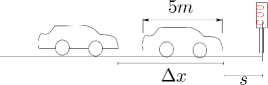
Figure 1: Initial setup

In this work, the problem of the optimal accommodation of cars on the line in front of a traffic signal is addressed. All drivers want to pass the crossing line before the green signal time is over, and to do that, they not only must be ready to accelerate as much as they can, but also they have to take an optimal position that maximize the flux through the crossing line. The used model consist in a line of $N$ identical cars of length $\ell$, taken as $5m$[25] for the most of this work. The response of the car is parametrized by the sensitivity parameter, so a slow response means a small $a$ value when a large $a$ represent a fast response. In this work, this parameter is taken in the range $a\in[0.2,2]s^{-1}$. The scale factor $d$ is taken as equal to the length of the car $\ell$. The maximum velocity $v_{\ell}$ is set to $13.88m/s\sim 50Km/h$, which is a speed typically accepted for urban area. The safe distance $d$ is a measure of how careful or careless (aggressive) is a driver. A system of aggressive drivers will set the safety distance small, which in this work is taken as $b\leq 0.7\ell$, instead a system of careful drivers would set $b>0.7\ell$. For the safety distance, the used values are $b\in[0.5,3]\ell$. And the green signal time duration is set in the range $t\in[20,120]s$, which is the usual range for urban area in Colombia.

Initially, the cars are equally spaced between them, except for the first one, that has its road clear (infinite headway). The first car starts from a distance $s=3m$ from the crossing line (see figure 1). Let’s call $x=0$ to the position that mark the crossing line of the signal, and the positive half-axis $x>0$ after the crossing line, i.e., all cars has negative initial position. The clock starts when the signal turns green and the system evolves following the dynamical rule in eq. 2. After the green time is over, the cars with positions $x_{n}>0$ have successfully passed through the signal crossing line. The position of each vehicle will be represented by a point in its front (see figure 1), so a headway $\Delta x$ equal or lesser than a vehicle length means that a collision has occurred, and it must be avoided.

4 Results and discussion.

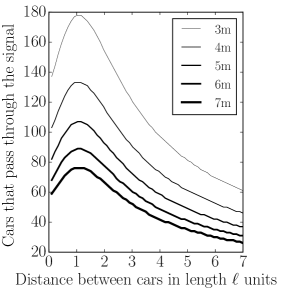
Figure 2: The optimal distance between cars in units of car length is always the same. Here a comparison among several car lengths, for a green time signal of $110$ seconds, $a=0.2s^{-1}$ and $b=0.5\ell$

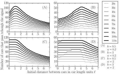
Figure 3: Count of cars that successfully pass through the signal crossing line, for several green time durations. For all computations the vehicle length is $\ell=5m$, $d=\ell$, $c=1$. The $b$ and $a$ parameters are stated for each graph in units of $\ell$ (car lenght) and $s^{-1}$ respectively

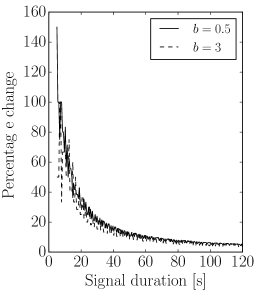
Figure 4: Percentage difference between the maximum number of cars that successfully passed through the green light signal, starting form the optimal separation, when increasing the sensitivity parameter from $a=0.2s^{-1}$ to $a=2s^{-1}$. $b$ values in units of car length $\ell$

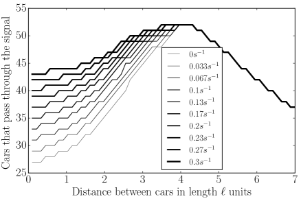
Figure 5: Introduction of the FVD term, for several values of $\lambda$. The sensitivity parameter is $a=0.2s^{-1}$, $b=3\ell$, $\ell=5m$.

First, the influence of the vehicle length in the optimal spacing has been tested, by holding constant the sensitivity and safety parameters and computing the number of vehicles that successfully pass through the signal crossing line, for a given green time period. The optimal separation between cars is defined as the distance that allows the maximum number of cars passing through the signal crossing line for a given green light time. In figure 2 the results are shown for a semaphore duration of $120s$, for several systems where the only difference is the length of the vehicles. Clearly, the smaller the cars are, the larger the number of cars that can successfully pass through, because the starting position of the $n$th car is closer to the line and each system is setup with the same sensitivity. Then it is expected for the flux peak to be larger for smaller cars. But it comes unexpected that the optimal separation, when normalized to the length of the vehicle, is always the same. These discovery justifies the normalization of distance to the vehicle length $\ell$ on further analysis.

Next, the influence of the sensitivity and the attitude of the drivers is studied. The number of cars that successfully pass through the crossing line of the signal, as a function of the separation between cars, for several green time lapses are shown in figure 3. Results for a small sensitivity parameter $a=0.2s^{-1}$ are shown in sub-figures $(A)$ and $(B)$, for safety distances of $b=0.5\ell$ and $b=3\ell$ respectively. And results for a high sensitivity system $a=2s^{-1}$ are presented in sub figures $(C)$ and $(D)$. It can be seen that the optimal separation between consecutive cars increases with the caution of the driver. A cautious driver starts slower when the leading car is close, and only feels comfortable accelerating if a large enough distance is separating the cars. Then, in order to increase its velocity fast enough, the initial separation must be large. In figure 3 for a $b=3\ell$ (sub figures $(B)$ and $(D)$), the maximum number of passing cars is obtained around a distance of $4\ell$ separating two consecutive cars. However, such large distance and the extreme caution of the drivers, prevent the system from having a large number of successful crossings. If the vehicles have a slow response, the flux is sub optimal for small distances between cars, increasing strongly when the system starts near the optimal separation. On the other hand, a set of aggressive drivers maximize the passing through the signal at lesser distances (one car length is optimal for $b=0.5\ell$). Surprisingly, the maximum optimal distance for maximum flux shows to be independent of the sensitivity parameter, being dependent only on the aggressive or careful behavior of the drivers. However, for large sensitivities, the range of distances that allows the system to obtain the maximum flux is wider. While the maximum flux do depend on both: the car sensitivity and the safe distance; for a fixed $b$ parameter the effect of an increasing on the sensitivity is an increment on the flux without changing the optimal distance. Such increase is larger for systems whose safety distance $b$ is farther from the region of optimal flux than when the $b$ parameter is closer to the optimal value. Then, the curves in figure 3 are softer when the sensitivity is larger. For separation distances larger than the optimal value, the effect of a better sensitivity is less important. To understand that, the reader must remember the “s” shape of the hyperbolic tangent function in eq. 3; at distances between cars for which the OV function is near its maximum, the nonlinearity of the hyperbolic tangent is not influencing considerably the behavior of the acceleration. Such effect is more evident for careful drivers (figure 3 (B) and (D)) than for aggressive ones (figure 3 (A) and (C)). However, the percentage difference between the maximum number of cars that successfully passed through the green light signal, starting from the optimal flux separation, is approximately independent from the safe distance at large signal durations (see figure 4). For small signal time durations, the discrete nature of the number of cars is manifested with oscillations in the percentage difference, however, a careful observer would notice that the central line of those oscillation is higher for aggressive drivers. Which means that for a short period of time, a set of aggressive drivers is more affected by a change on the sensitivity parameter than a system of careful ones, when starting from the optimal distance. However, over time, the effect of safety distance is dismissed and the increase on sensitivity provides the same effect on every system. That can be easy understood: as time goes on, the vehicles are reaching its optimal velocity, so the flux gets stabilized to the same number of cars by unit of time, independently of the sensitivity and the safety parameters.

4.1 Computations with an improved model

The computations were redone under the light of the full velocity differences model. The parameters used were $\lambda\in[0,0.36]$. When the zero value is used, the model corresponds to the original OV model of eq. 2. In was found that the previous findings holds. The optimal distance between cars remains unchanged when the $\lambda$ parameter is included. The effect of the FVD term is the increasing of the flux for systems starting from suboptimal separations (see figure 5). Those arrangements of cars starting with distance between cars equal to the optimal separation or bigger, get not changed at all for the range of $\lambda$ studied.

The FVDOV model takes into account not only the headway, but also the relative velocity when selecting the optimal speed. Then, if the driver sees that his leader is starting faster than he is, a higher acceleration is possible, that makes the starting process faster and the flux through the signal for small initial distances is increased. However, the initial separation between cars is determinant in the system acceleration and velocity; as every vehicle but the first one starts under equal initial conditions, then their acceleration is initially the same. Only the leader starts without obstacles in his way, so the velocity difference between the $n$th car and the $(n+1)$th is getting smaller as $n$ increase. As a consequence, for initial distances equal or larger than the optimal separation, the acceleration due to the OV velocity function is determinant up to the free flow speed is achieved. In this process, the relative velocity term is just a small perturbation and the curve in figure 5 is unchanged.

5 Conclusions

A comprehensive study on the effects of vehicles separation on the flux through a signal light has been performed. The models used has been based on the Bando’s optimal velocity model, with open boundaries, and the improved model known as Full Velocity Differences. The model consist on $N$ identical cars, in a line, equally spaced in front of a signal, with no obstacles after. It was found that the separation between cars is indeed determinant on the flux capacity of the signal. Clearly, a too large initial separation do not benefit the flux, but contrary to what seems to be the common thinking, a too small separation prevents the system from getting the maximum number of cars successfully passing through the signal. The sensitivity of the systems has been found not to cause a perceptible change on the flux, when the attitude of the drivers is determinant. Systems with aggressive drivers are found to have small initial optimal separation. Surprisingly, the optimal separation between consecutive cars in terms of its length, is a constant for each system, i.e., is independent of the length of the car for a given configuration (parameters $a,b,c,v_{\ell}$ of the model). The increase on the sensitivity affects the number of successfully passing cars, but not the optimal initial separation. However, such increment is more significant when the system starts from a suboptimal separation. It was also found that for systems starting from the optimal initial separation, the percentage increment on the number of cars that cross through the signal is approximately independent of the attitude for large signal durations, when for short times it is larger for aggressive drivers.

6 Acknowledgement

Founding: This research has been supported by Universidad del Altántico.

References

References

-
[1]
M. Bando, K. Hasebe, A. Nakayama, A. Shibata, Y. Sugiyama,
Dynamical model of
traffic congestion and numerical simulation, Phys. Rev. E 51 (1995)
1035–1042.
doi:10.1103/PhysRevE.51.1035.
URL http://link.aps.org/doi/10.1103/PhysRevE.51.1035 -
[2]
M. Bando, K. Hasebe, K. Nakanishi, A. Nakayama,
Analysis of optimal
velocity model with explicit delay, Phys. Rev. E 58 (1998) 5429–5435.
doi:10.1103/PhysRevE.58.5429.
URL http://link.aps.org/doi/10.1103/PhysRevE.58.5429 -
[3]
L. Davis,
Modifications
of the optimal velocity traffic model to include delay due to driver reaction
time, Physica A: Statistical Mechanics and its Applications 319 (2003) 557
– 567.
doi:http://dx.doi.org/10.1016/S0378-4371(02)01457-7.
URL http://www.sciencedirect.com/science/article/pii/S0378437102014577 -
[4]
H. Ez-Zahraouy, Z. Benrihane, A. Benyoussef,