AWGN-Goodness is Enough: Capacity-Achieving Lattice Codes based on Dithered Probabilistic Shaping

Abstract

In this paper we show that any sequence of infinite lattice constellations which is good for the unconstrained Gaussian channel can be shaped into a capacity-achieving sequence of codes for the power-constrained Gaussian channel under lattice decoding and non-uniform signalling. Unlike previous results in the literature, our scheme holds with no extra condition on the lattices (e.g. quantization-goodness or vanishing flatness factor), thus establishing a direct implication between AWGN-goodness, in the sense of Poltyrev, and capacity-achieving codes. Our analysis uses properties of the discrete Gaussian distribution in order to obtain precise bounds on the probability of error and achievable rates. In particular, we obtain a simple characterization of the finite-blocklength behavior of the scheme, showing that it approaches the optimal dispersion coefficient for high signal-to-noise ratio. We further show that for low signal-to-noise ratio the discrete Gaussian over centered lattice constellations cannot achieve capacity, and thus a shift (or “dither”) is essentially necessary.

I Introduction

Coded modulation schemes for the Gaussian channel can be usually constructed from infinite constellations (ICs) in $\mathbb{R}^{n}$, shaped according to the power constraint of the channel. In order to analyse such infinite constellations independently of the power, Poltyrev [23] defined the notion of codes which are good for the unconstrained Gaussian channel. In this setting, a code is an infinite discrete subset of $\mathbb{R}^{n}$, and any point can be transmitted. Since the usual code rate is infinite in this case, the optimal normalized log density (NLD) replaces the notion of capacity. The NLD measures the logarithm, per dimension, of the number of points of an IC per unit of volume. An optimal sequence of ICs with vanishing probability of error is called AWGN-good, and corresponds to the “most economic” constellations that can achieve reliable communication. The most popular ICs are lattices, since their symmetries allow for construction of efficient encoding/decoding schemes. Since the work of Poltyrev in 1994, the notion of AWGN-goodness has become an important widely used benchmark and building block for the construction of lattice codes.

Intuitively, AWGN-good ICs should be able to produce capacity-achieving codes in the power-constrained setting, using nearest neighbor decoding and a carefully chosen shaping technique. Nevertheless, all known schemes in the literature that convert lattices into codes for the constrained Gaussian channel under lattice decoding entail some additional property. For instance, Erez and Zamir [10] proved that an AWGN-good sequence of lattices can be converted into capacity-achieving codes for the Gaussian channel, provided that it can be nested to another lattice sequence which is also AWGN-good and has optimal normalized second-moment (i.e., quantization-good). Recently, Ling and Belfiore [17] have shown that a sequence of lattices along with probabilistic shaping can achieve the capacity of the Gaussian channel above a certain signal-to-noise ratio (SNR) provided that it has vanishing flatness factor, which relates to how quickly a Gaussian random vector becomes equidistributed over cosets of the lattice as its standard deviation increases.

The objective of this paper is to show that indeed AWGN-goodness is a sufficient property for building capacity-achieving lattices in the Gaussian channel, with no extra condition. In order to do so, we employ a technique based on non-equiprobable signalling using discrete Gaussian distributions centered at a (non-zero) randomly generated point in $\mathbb{R}^{n}$. Following [22], we call such technique dithered probabilistic shaping (DPS). From a practical “separation” point of view, this means that the design problem of good lattices for the AWGN channel can be completely decoupled: one can focus entirely on the design problem for the unconstrained channel, which can be then coupled with plug-and-play DPS techniques into a good code for the constrained channel.

I-A Main Result

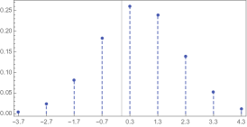
(a) A one-dimensional discrete Gaussian with support in $\mathbb{Z}+0.3$

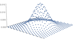
(b) A two-dimensional centered discrete Gaussian with support in a hexagonal lattice

Figure 1: Illustration of the discrete Gaussian distribution

Let $\mathbf{W}\sim\mathcal{N}(\mathbf{0},\sigma_{w}^{2})$ be an $n$-dimensional Gaussian random vector. A sequence of AWGN-good lattices $(\Lambda_{n})_{n=1}^{\infty}$ with volume $V(\Lambda_{n})$ is such that the probability of error (i.e. the probability that $\mathbf{W}$ leaves the Voronoi cell of $\Lambda_{n}$) vanishes for any NLD

$$\delta(\Lambda_{n})\triangleq-\frac{1}{n}\log V(\Lambda_{n})<-\frac{1}{2}\log(2\pi e\sigma_{w}^{2})\triangleq\delta^{*}.$$ (1)

The discrete Gaussian distribution $\mathcal{D}_{\Lambda+\mathbf{t},\sigma_{s}^{2}}$ is the distribution taking values in $\Lambda+\mathbf{t}$ whose mass of $\mathbf{x}+\mathbf{t}$ is proportional to $e^{-\left\|\mathbf{x}+\mathbf{t}\right\|/2\sigma_{s}^{2}}$ (see Figure 1). This distribution has finite power and can thus be used in the transmission over a Gaussian channel with average power constraint $P$. In a lattice Gaussian coding scheme, the sent signal is chosen according to $\mathcal{D}_{\Lambda+\mathbf{t},\sigma_{s}}$, while the received points are suitably scaled and then decoded using lattice decoding.

Let $(\Lambda_{n})_{n=1}^{\infty}$ be a sequence of AWGN-good lattices. Our main result states the existence of a sequence of shift vectors (or “dithers”) $(\mathbf{t}_{n})_{n=1}^{\infty}$ such that the lattice coding scheme with distribution $\mathcal{D}_{\Lambda_{n}+\mathbf{t}_{n},\sqrt{P}}$ is capacity-achieving in the Gaussian channel. A more quantitative statement can be found in Theorem 1, along with an analysis of the rate of convergence to capacity. For instance, we show that the existence of $\mathbf{t}_{n}$ holds with constant probability and, using [15], that the gap to capacity has order $\approx(2n)^{-1/2}(Q^{-1}(\varepsilon)+\sqrt{8})$ where $Q^{-1}$ is the inverse-error function. Apart for the $\sqrt{8}$ term (which we believe is an artifact of our analysis), this corresponds to the optimal convergence behavior for the Gaussian channel for high SNR [24]. In particular, as $\varepsilon\to 0$, the optimal dispersion is approached at high SNR.

A key point for the proof of the main results is the sampling lemma (Lemma 2), that says that the dithered lattice Gaussian is equivalent to a continuous Gaussian. Since continuous dithers would require sharing an infinite number of random bits, we then demonstrate the sufficiency of discrete dithering in Lemma 7. As a further point of interest, we observe using [7] that the coding gain of a lattice is closely related to the so-called smoothing parameter of the dual lattice. At a high level, the discrete Gaussian over dual lattice $\Lambda^{*}$ sampled above the smoothing parameter “looks like” a continuous Gaussian, which justifies the name. The study of this parameter has played a fundamental role in our understanding of the discrete Gaussian, and has led to many important developments such as tight transference theorems in the geometry of numbers [1], new lattice based cryptographic schemes [20, 26, 13], and the recent development of the so-called reverse Minkowski inequality [27, 28]. This relation, discussed in Section IV, gives an alternative viewpoint for quantifying AWGN-goodness that we hope will find future use.

I-B To Dither or Not to Dither

Since the seminal work [10], nested lattice constellations are known to be capacity achieving in the Gaussian channel with lattice decoding, provided that the constellations are suitably shifted by a vector known both at the transmitter and at the receiver. The process of randomizing the choice of the shift vector, known as dithering, greatly facilitates the analysis but may introduce additional design complexity. An intriguing open problem is whether dithering is indeed necessary. For Voronoi constellations (under MMSE scaled lattice decoding), this problem is considered in [32, 33], where the necessity of a dither is argued for low SNR.

Recently, Ling and Belfiore [17] have shown that undithered lattice coding, with probabilistic shaping according to a discrete Gaussian distribution, is capacity achieving for a threshold SNR greater than $e$. In another work [9], di Pietro, Zemor and Boutros showed that LDA lattices without dithering achieve capacity on the Gaussian channel if SNR $>1$. In Section V of the present paper, we show that (a non-zero) dither is indeed necessary in the low SNR regime. Specifically we show (Theorem 2) that if a sequence of lattices is shaped according to a centered Gaussian distribution with variance parameter equals to the power constraint of the channel, it fails to achieve any positive rates for $\text{SNR}<1$. Interestingly, in the low SNR regime our scheme uses properties of the discrete Gaussian when the flatness factor is large (or “below smoothing”, in the computer science jargon), a setting where previous analytical techniques break down. As it turns out, in this regime, dithering is not only a matter of simplification but essentially necessary. It is noting that although polar lattices [31] can achieve capacity for all SNRs, their construction employ randomly generated bits which, ultimately, play the role of a dither.

I-C Related Works

In comparison to previous works on nested lattice constellations [10], approaches based on discrete Gaussians do not rely on a quantization-good sub-lattice for shaping. It is worth noting that, since [10], there has been a significant effort employed in simplifying nested-lattice constellations. For instance, [21] removes the assumption that the shaping sub-lattice needs to be AWGN-good and [25] by-passes the quantization-good by using a discrete dither and removing the constellation points with large power. Relying on the machinery of the discrete Gaussian distribution, our approach removes the reliance on a sub-lattice with suitable properties, and greatly simplifies the proof that lattice codes are capacity-achieving in the Gaussian channel (our full proof is self-contained in Section III).

Our main result strongly uses non-uniform signalling, which could be implemented with probabilistic shaping techniques. In a broader scope, besides the theoretically appealing properties of probabilistic shaping for Gaussian channels [16],[17], the techniques became popular in the last years due to their prospective applications to non-linear optical-fiber transmissions [11], [29]. The idea of dithered probabilistic shaping (DPS) was previously considered in [22], who proposed a method to achieve high shaping gains of a constellation with small dimension and low complexity.

Besides showing the sufficiency of the AWGN goodness figure of merit, our analysis closes the gap of uniform signalling [17] for low SNR. Although this is not the usual regime for wireless channels, it has attracted a recent interest due to secrecy applications in low profile covert communications [30, 4, 3], where signals are transmitted with very low power. Understanding how probabilistic shaping schemes behave for low SNR might find use in such scenarios. In addition to AWGN channel coding, there is an increasing literature in the use of the discrete Gaussian in other information-theoretic scenarios where our simplified approach could play a role. A few examples are Gaussian wiretap channels [18], fading wiretap channels [19], and compound channels [6].

II Notation and Preliminary Results

We consider a real-valued AWGN channel with average-power constraint $P$ and noise variance $\sigma_{w}^{2}$. Denote the received signal of the channel, given input $\mathbf{x}\in\mathbb{R}^{n}$, by $\mathbf{y}=\mathbf{x}+\mathbf{w}$, where $\mathbf{w}$ is drawn from the distribution $\mathcal{N}(0,\sigma_{w}^{2}\mathbf{I}_{n})$. A (full-rank) lattice $\Lambda\subset\mathbb{R}^{n}$ is a discrete subgroup not contained in any proper subspace of $\mathbb{R}^{n}$.

Definition 1.

A lattice code for the Gaussian channel consists of

1. A lattice $\Lambda\subset\mathbb{R}^{n}$.

2. A finite-entropy probability distribution $\mathcal{D}$ taking values in $\Lambda$ such that, for $\mathbf{X}\sim\mathcal{D},E[\left\|\mathbf{X}\right\|^{2}]\leq nP.$

3. A decoding function $g:\mathbb{R}^{n}\to\Lambda$.

The error probability of a lattice code is $P_{e}(\Lambda)\triangleq\Pr(g(\mathbf{X}+\mathbf{W})\neq\mathbf{X})$, where $\mathbf{W}\sim\mathcal{N}(0,\sigma_{w}^{2}\mathbf{I}_{n})$. The rate of the code is given by $R=(1/n)\mathbb{H}(\mathbf{X}),$ where

$$\mathbb{H}(\mathbf{X})\triangleq-\sum_{\mathbf{x}\in\Lambda}\Pr(\mathbf{X}=\mathbf{x})\log\Pr(\mathbf{X}=\mathbf{x})$$

is the entropy of distribution $\mathcal{D}$ (all logarithms are with respect to base $e$ and rates are calculated in nats). We can similarly define lattice codes for a translation $\Lambda+\mathbf{t}$, where $\mathbf{t}\notin\Lambda$, with the obvious modifications.

If $\mathcal{D}$ is the uniform distribution over the points of $\Lambda$ in a compact set $\mathcal{S}$ (e.g. a ball or the Voronoi region of a sub-lattice), and zero otherwise, this corresponds to the classic “deterministic” shaping. In this case, a set of possible uniformly distributed messages $\left\{1,2,\ldots,e^{nR}\right\}$ can be mapped into the signal space by simply labeling the points in $\Lambda\cap\mathcal{S}$. When $\mathcal{D}$ is non-uniform, messages can be mapped into the signal space by means of probabilistic shaping techniques (e.g. [22], [17, Sec IV][5], [33, Sec 6.5]).

Let $\text{SNR}\triangleq P/\sigma_{w}^{2}$ and $C(\text{SNR})\triangleq 1/2\log(1+\text{SNR})$.

Definition 2.

A sequence of lattice codes of increasing dimension $\Lambda_{n}$ with distributions $\mathcal{D}_{n}$ is said to be capacity-achieving in the Gaussian channel with $\text{{SNR}}=P/\sigma_{w}^{2}$ if $P_{e}(\Lambda_{n})\to 0$ and

$$\lim_{n\to\infty}\frac{1}{n}\mathbb{H}(\mathbf{X}_{n})=C(\text{{SNR}}),$$ (2)

where $\mathbf{X}_{n}\sim\mathcal{D}_{n}$.

Definition 3.

Let

$$f_{\sigma}(\mathbf{x})=\frac{e^{-\left\|\mathbf{x}\right\|^{2}/2\sigma^{2}}}{(\sqrt{2\pi\sigma^{2}})^{n}}.$$

The discrete Gaussian distribution $\mathcal{D}_{\Lambda+\mathbf{t},\sigma}$ is the discrete distribution assuming values in $\Lambda+\mathbf{t}$ such that the mass of each point $\mathbf{x}+\mathbf{t}\in\Lambda+\mathbf{t}$ is proportional to $f_{\sigma}(\mathbf{x}+\mathbf{t})$.

If $\mathcal{D}$ in Definition 1 is a discrete Gaussian distribution assuming values in $\Lambda+\mathbf{t}$, the corresponding code is called a lattice Gaussian code. Some discrete Gaussians are illustrated in Figure 1. If a point in a lattice Gaussian code is transmitted over a Gaussian channel, we have the following fact:

Lemma 1 (Equivalence between MAP and lattice decoder [17]).

Let $\hat{\mathbf{x}}$ be the output of the maximum-a-posteriori decoder for a lattice Gaussian code with distribution $\mathcal{D}_{\Lambda+\mathbf{t},\sigma_{s}^{2}}$. We have

$$\hat{\mathbf{x}}=\displaystyle\arg\min_{\mathbf{x}\in\Lambda+\mathbf{t}}\left\|\alpha\mathbf{y}-\mathbf{x}\right\|,$$

where $\alpha=\sigma_{s}^{2}/(\sigma_{s}^{2}+\sigma_{w}^{2})$ is called the MMSE (or Wiener) coefficient.

Therefore, the optimal MAP decoder is obtained by MMSE pre-processing followed by lattice decoding. Let $\mathbf{W}_{\text{{eff}}}=(\alpha-1)\mathbf{X}+\alpha\mathbf{W}$ be the effective noise in this process. For an $n$-dimensional lattice $\Lambda\subset\mathbb{R}^{n}$, we define the Voronoi cell $\mathcal{V}(\Lambda)$ of $\Lambda$ by

$$\mathcal{V}(\Lambda)=\left\{\mathbf{x}\in\mathbb{R}^{n}:\langle\mathbf{x},\mathbf{y}\rangle\leq\|\mathbf{y}\|^{2}/2\text{, for any }\mathbf{y}\in\Lambda\right\}$$

namely, the set of all points closer to the origin than any other lattice point. The volume of $\Lambda$, denoted by $V(\Lambda)$, corresponds to the volume of the Voronoi cell $\mathcal{V}(\Lambda)$. From Lemma 1, the probability of error of the maximum-a-posteriori decoder is

$$P_{e}(\Lambda)=\Pr(\mathbf{W}_{\text{{eff}}}\notin\mathcal{V}(\Lambda)).$$

We denote by $\mathbf{x}\mbox{ mod}\Lambda$ the unique representative of $\mathbf{x}\in\mathbb{R}^{n}$ in the voronoi cell of $\Lambda$, with ties broken arbitrarily.

III Capacity Achieving Codes From AWGN-Good Lattices

In this section, we will show that any AWGN-good lattice $\Lambda$ can be used to construct a capacity achieving code for the AWGN-channel. The caveat will be the use of a random dither as well as the use of non-equiprobable encoding, namely discrete Gaussian encoding. We will later argue in in Section IV that a discrete dither suffices and in Section V that the dither is essentially necessary for this construction to hold for all SNR.

Let us now examine an ensemble of coding schemes in $\mathbb{R}^{n}$ based on a $n$-dimensional lattice $\Lambda\subset\mathbb{R}^{n}$. Define the inverse error function of $\Lambda$ by

$${\rm err}^{-1}_{\varepsilon}(\Lambda)=\min\left\{s:\Pr_{\mathbf{x}\sim\mathcal{N}(\mathbf{0},\mathbf{I}_{n})}[x\notin s\mathcal{V}(\Lambda)]\leq\varepsilon\right\}\text{ .}$$ (3)

Note that for a AWGN-good family $(\Lambda_{n})_{n=1}^{\infty}$, $V(\Lambda_{n})=1~{}\forall i\in[n]$, for any fixed $\varepsilon>0$ we have that $\lim_{n\rightarrow\infty}{\rm err}^{-1}_{\varepsilon}(\Lambda)\rightarrow\sqrt{2\pi e}$. We also define the normalized volume-to-noise ratio (NVNR) of lattice at probability of error $\varepsilon$ as:

$$\mu(\Lambda,\varepsilon)={{\rm err}^{-1}_{\varepsilon}(\Lambda)^{2}V(\Lambda)^{2/n}}.$$ (4)

This definition indeed corresponds to the usual NVNR (e.g. [33, Def. 3.3.3]), rephrased in light of the error function (3). For convenience, we further normalize $\mu(\Lambda,\varepsilon)$ by $2\pi e$ and define

$$\gamma(\Lambda,\varepsilon)=\frac{\mu(\Lambda,\varepsilon)}{2\pi e}.$$ (5)

This ratio can be interpreted as the “modulation loss” of $\Lambda$. For an AWGN-good sequence, $\log\gamma(\Lambda_{n},\varepsilon)$ vanishes as $n\to\infty$.

Let $\sigma_{s}^{2}$, $\sigma_{w}^{2}$ denote the nominal power of the signal and the noise power per symbol respectively and let $\sigma_{{\rm eff}}^{2}:=\frac{\sigma_{s}^{2}\sigma_{w}^{2}}{\sigma_{s}^{2}+\sigma_{w}^{2}}$.

Let $\Lambda\subset\mathbb{R}^{n}$ be a lattice. Given a fixed probability of error $\varepsilon>0$, we will now examine a family of dithered coding schemes which on average have decoding error at most $6\varepsilon$, power per symbol $\leq\sigma_{s}^{2}(1+4/\sqrt{n})$, and gap to the capacity depending only on the relationship between the inverse error function and the lattice determinant. The existence of a good code from our family will then follow by the union bound appropriately applied.

For the purpose of finding a good code, we shall examine the family of encoding distributions $D_{\Lambda+\mathbf{t},\sigma_{s}}$, indexed by $\mathbf{t}\in\mathbb{R}^{n}$, i.e. the discrete Gaussian on $\Lambda+\mathbf{t}$ of parameter $\sigma_{s}$. For a given $\mathbf{t}$, the decoding function $g_{\mathbf{t}}$ will be maximum a posteriori decoding as in Lemma 1, namely for a noisy signal $\mathbf{y}\in\mathbb{R}^{n}$, the decoded signal corresponds to

$$g_{\mathbf{t}}(\mathbf{y}):=\arg\min_{\mathbf{x}\in\Lambda+\mathbf{t}}\left\|\mathbf{x}-\frac{\sigma_{s}^{2}}{\sigma_{s}^{2}+\sigma_{w}^{2}}\mathbf{y}\right\|\text{ .}$$

To prove our bounds on the average properties of such codes we need a distribution on shifts $\mathbf{t}$. For this distribution, we pick the natural choice $\mathbf{T}\sim\mathcal{N}(\mathbf{0},\sigma_{s}^{2}\mathbb{I}_{n})$, i.e. the shift is distributed according to the maximum entropy input distribution satisfying the average power constraint.

The main theorem we will prove in this section is as follows.

Theorem 1.

Let $\Lambda\subset\mathbb{R}^{n}$ be an $n$-dimensional lattice, $n\geq 16$. For power $\sigma_{s}^{2}=P$, noise variance $\sigma_{w}^{2}>0$ and probability of error $\varepsilon>0$, let $\sigma_{\rm eff}^{2}=\frac{\sigma_{s}^{2}\sigma_{w}^{2}}{\sigma_{s}^{2}+\sigma_{w}^{2}}$, $s_{\varepsilon}={\rm err}^{-1}_{\varepsilon}(\Lambda)\cdot\sigma_{\rm eff}$ and $\gamma(\Lambda,\varepsilon)={\rm err}^{-1}_{\varepsilon}(\Lambda)^{2}V(\Lambda)^{2/n}/(2\pi e)$. Then for $\mathbf{T}\sim\mathcal{N}(\mathbf{0},\sigma_{s}^{2}\mathbb{I}_{n})$ with probability at least $1/2$ the coding distribution $\mathbf{X}\sim D_{s_{\varepsilon}\Lambda+\mathbf{T},\sigma_{s}}$ equipped with maximum likelihood decoding satisfies:

1. The decoding error is bounded by $6\varepsilon$.

2. The squared power per symbol is at most $(1+4/\sqrt{n})\sigma_{s}^{2}$.

3. The per symbol gap to capacity is bounded by $\frac{1}{2}\log\gamma(\Lambda,\varepsilon)+\frac{2}{\sqrt{n}}+\frac{4}{n}$.

For notational convenience, we will assume in the remainder that $\sigma_{\rm eff}\cdot{\rm err}^{-1}_{\varepsilon}(\Lambda)=1$ (note that this can be achieved by simply scaling the lattice). With this normalization, we will be able to achieve a low probability of error by choosing the codes directly from $\Lambda$ (instead of a scaling of $\Lambda$).

To prove the theorem, we will rely on the subsequent lemmas which characterize the behavior of a randomly dithered channel. We first present these lemmas and prove Theorem 1 at the end of the section.

The following simple sampling lemma shows the random variables corresponding to either sampling $\mathbf{T}$ from $\mathcal{N}(\mathbf{0},\sigma_{s}^{2}\mathbb{I}_{n})$ and a) returning $\mathbf{T}$ or b) returning a discrete Gaussian sample from $D_{\Lambda+\mathbf{T},\sigma_{s}}$ have the same distribution.

Lemma 2 (Sampling Lemma).

Let $\mathbf{T}\sim\mathcal{N}(\mathbf{0},\sigma_{s}^{2}\mathbb{I}_{n})$ and let $\mathbf{X}\sim D_{\Lambda+\mathbf{T},\sigma_{s}}$. Then $\mathbf{T}$ and $\mathbf{X}$ are identically distributed.

Proof.

We need only show that $\mathbf{X}$ has the same probability density as $\mathbf{T}$. For $\mathbf{w}\in\mathbb{R}^{n}$, note that $\mathbf{X}$ can only hit $\mathbf{w}$ if $\mathbf{w}\in\Lambda+\mathbf{T}\Leftrightarrow\mathbf{T}\in\Lambda+\mathbf{w}$. Therefore, for any measurable set $A\subseteq\mathbb{R}^{n}$, we have that

$$\Pr[\mathbf{X}\in A] =\int_{\mathbb{R}^{n}}f_{\sigma_{s}}(\mathbf{t})\Pr[\mathbf{X}\in A|T=\mathbf{t}]{d\mathbf{t}}$$

$$=\int_{\mathbb{R}^{n}}f_{\sigma_{s}}(\mathbf{t})\frac{f_{\sigma_{s}}(A\cap(\Lambda+\mathbf{t}))}{f_{\sigma_{s}}(\Lambda+\mathbf{t})}{d\mathbf{t}}$$

$$=\int_{\mathcal{V}(\Lambda)}\sum_{\mathbf{x}\in\Lambda+\mathbf{c}}f_{\sigma_{s}}(\mathbf{x})\frac{f_{\sigma_{s}}(A\cap(\Lambda+\mathbf{c}))}{f_{\sigma_{s}}(\Lambda+\mathbf{c})}{d\mathbf{c}}$$

$$=\int_{\mathcal{V}(\Lambda)}f_{\sigma_{s}}(A\cap(\Lambda+\mathbf{c})){d\mathbf{c}}=\int_{A}f_{\sigma_{s}}(\mathbf{x}){d\mathbf{x}}\text{, }$$

as needed. ∎

Remark 1.

Note that the sampling lemma still holds if we take $\mathbf{T}\sim\mathcal{N}(0,\sigma_{s}^{2}\mathbb{I}_{n})\text{ {mod} }\Lambda$, where the mod-$\Lambda$ operation maps a point in $\mathbb{R}^{n}$ to a coset representative in the Voronoi cell of $\Lambda$. The $\ell_{\infty}$ distance between $\mathcal{N}(0,\sigma_{s}^{2}\mathbb{I}_{n})\text{ {mod} }\Lambda$ and a uniform distribution in $\mathcal{V}(\Lambda)$, normalized by $1/V(\Lambda)$, is the so-called flatness factor (e.g. [17]). If the flatness factor of $\Lambda$ is small, roughly speaking, one could replace $\mathbf{T}$ in Lemma 2 by a uniform dither. As we will see later in Section V, this condition is too stringent for low SNR.

We now show that expected probability of error of our lattice family is exactly $\varepsilon$. In what follows, $\mathbf{T}\sim\mathcal{N}(\mathbf{0},\sigma_{s}^{2}\mathbb{I}_{n})$ will be our random shift of $\Lambda$, $\mathbf{W}\sim\mathcal{N}(\mathbf{0},\sigma_{w}^{2}\mathbb{I}_{n})$ will be the channel noise, $\mathbf{X}\sim D_{\Lambda+\mathbf{T},\sigma_{s}}$ will denote the coding distribution, and $g_{\mathbf{T}}$ is our decoding function. We recall our assumption that $\sigma_{{\rm eff}}\cdot{\rm err}^{-1}_{\varepsilon}(\Lambda)=1$.

Lemma 3 (Error Probability Bound).

For $\gamma\geq 1$,

$$\Pr_{\mathbf{T}}[\Pr_{\mathbf{X}}[g_{\mathbf{T}}(\mathbf{X}+\mathbf{W})\neq\mathbf{X}]\geq\gamma\varepsilon]\leq 1/\gamma\text{ .}$$

Proof.

Let $\alpha=\frac{\sigma_{s}^{2}}{\sigma_{s}^{2}+\sigma_{w}^{2}}$. Recall that $g_{\mathbf{T}}(\mathbf{X}+\mathbf{W})\neq\mathbf{X}$ if and only if

$$(1-\alpha)\mathbf{X}+\alpha\mathbf{W}\notin\mathcal{V}(\Lambda)\text{ .}$$

By the sampling lemma $\mathbf{X}$ has distribution $\mathcal{N}(\mathbf{0},\sigma_{s}^{2}\mathbb{I}_{n})$. Given that $\mathbf{X}$ and $\mathbf{W}$ are independent Gaussians, we have that $(1-\alpha)\mathbf{X}+\alpha\mathbf{W}$ is distributed as $\mathcal{N}(\mathbf{0},\sigma_{\rm eff}^{2}\mathbb{I}_{n})$ since by construction

$$\sigma_{{\rm eff}}^{2}:=\frac{\sigma_{s}^{2}\sigma_{w}^{2}}{\sigma_{s}^{2}+\sigma_{w}^{2}}=(1-\alpha)^{2}\sigma_{s}^{2}+\alpha^{2}\sigma_{w}^{2}\text{ .}$$

By assumption on $\Lambda$ we have that $\sigma_{\rm eff}\cdot{\rm err}^{-1}_{\varepsilon}(\Lambda)=1$, and thus

$$\Pr[(1-\alpha)\mathbf{X}+\alpha\mathbf{W}\notin\mathcal{V}(\Lambda)] =\Pr_{\mathbf{Z}\sim\mathcal{N}(\mathbf{0},\mathbb{I}_{n})}[\sigma_{\rm eff}\mathbf{Z}\notin\mathcal{V}(\Lambda)]$$

$$=\Pr_{\mathbf{Z}\sim\mathcal{N}(\mathbf{0},\mathbb{I}_{n})}[\mathbf{Z}\notin{\rm err}^{-1}_{\varepsilon}(\Lambda)\mathcal{V}(\Lambda)]=\varepsilon\text{ .}$$

Using the above, by Markov’s inequality we have that

$$\Pr_{\mathbf{T}}[\Pr_{\mathbf{X}}[g_{\mathbf{T}}(\mathbf{X}+\mathbf{W})\neq\mathbf{X}]\geq\gamma\varepsilon]\leq\frac{\Pr[g_{\mathbf{T}}(\mathbf{X}+\mathbf{W})\neq\mathbf{X}]}{\gamma\varepsilon}=\frac{1}{\gamma}\text{ ,}$$

as needed. ∎

The next lemma shows that average power per symbol is very close to the desired limit. The proof proceeds by a comparison to the continuous Gaussian followed by a standard Chernoff bound.

Lemma 4.

For any $\varepsilon>0$, we have that

$$1.\Pr_{\mathbf{T}}[\mathbb{E}[\|(\mathbf{X}/\sigma_{s})\|^{2}|\mathbf{T}]]\geq(1+\varepsilon)n]\leq e^{-(\varepsilon^{2}/4-\varepsilon^{3}/6)n}$$

$$2.\Pr_{\mathbf{T}}[\mathbb{E}[\|(\mathbf{X}/\sigma_{s})\|^{2}|\mathbf{T}]]\leq(1-\varepsilon)n]\leq e^{-(\varepsilon^{2}/4+\varepsilon^{3}/6)n}$$

Proof.

We first prove the upper bound. Since $\mathbf{X}/\sigma_{s}\sim\mathcal{N}(0,\mathbb{I}_{n})$, a standard computation reveals that $\mathbb{E}[e^{\alpha\|\mathbf{X}/\sigma_{s}\|^{2}}]=(1-2\alpha)^{-n/2}$ for $\alpha<1/2$. By the Chernoff bound

$$\begin{split}\Pr_{\mathbf{T}}[\mathbb{E}[\|(\mathbf{X}/\sigma_{s})\|^{2}|\mathbf{T}]\geq(1+\varepsilon)n]&\leq\min_{\alpha\in(0,1/2)}\frac{\mathbb{E}_{\mathbf{T}}[e^{\alpha\mathbb{E}[\|(\mathbf{X}/\sigma_{s})\|^{2}|\mathbf{T}]}]}{e^{\alpha(1+\varepsilon)n}}\\ &\leq\min_{\alpha\in(0,1/2)}\frac{\mathbb{E}[e^{\alpha\|(\mathbf{X}/\sigma_{s})\|^{2}}]}{e^{\alpha(1+\varepsilon)n}}\quad\left(\text{ by Jensen's inequality }\right)\\ &=\min_{\alpha\in(0,1/2)}\left(\frac{e^{-(1+\varepsilon)\alpha}}{\sqrt{1-2\alpha}}\right)^{n}\\ &=(\sqrt{1+\varepsilon}e^{-\varepsilon/2})^{n}<e^{-(\varepsilon^{2}/4-\varepsilon^{3}/6)n}\left(\text{ setting $\alpha=\frac{\varepsilon}{2(1+\varepsilon)}$ }\right)\text{ .}\end{split}$$

Similarly, for the lower bound, we have

$$\Pr_{\mathbf{T}}[\mathbb{E}[\|(\mathbf{X}/\sigma_{s})\|^{2}|\mathbf{T}]\leq(1-\varepsilon)n] \leq\min_{\alpha>0}\frac{\mathbb{E}_{\mathbf{T}}[e^{-\alpha\mathbb{E}[\|(\mathbf{X}/\sigma_{s})\|^{2}|\mathbf{T}]}]}{e^{-\alpha(1-\varepsilon)n}}$$

$$\leq\min_{\alpha>0}\frac{\mathbb{E}[e^{-\alpha\|(\mathbf{X}/\sigma_{s})\|^{2}}]}{e^{\alpha(1-\varepsilon)n}}\quad\left(\text{ by Jensen's inequality }\right)$$

$$=\min_{\alpha>0}\left(\frac{e^{(1-\varepsilon)\alpha}}{\sqrt{1+2\alpha}}\right)^{n}$$

$$=(\sqrt{1-\varepsilon}e^{\varepsilon/2})^{n}<e^{-(\varepsilon^{2}/4+\varepsilon^{3}/6)n}\left(\text{ setting $\alpha=\frac{\varepsilon}{2(1-\varepsilon)}$ }\right)\text{ .}$$

∎

We now argue that the entropy of the coding distribution is large with good probability. In particular, we would like to know that for most choices $\mathbf{t}$ for $\mathbf{T}$ that $\mathbb{H}(\mathbf{X}|\mathbf{T}=\mathbf{t})$ is large. Recall that $\mathbf{X}|\mathbf{T}=\mathbf{t}$ is distributed as $D_{\Lambda+\mathbf{t},\sigma_{s}}$, where a direct computation gives

$$\begin{split}\mathbb{H}(\mathbf{X}|\mathbf{T}=\mathbf{t})&=\sum_{\mathbf{y}\in\Lambda+\mathbf{t}}-\log\left(\frac{f_{\sigma_{s}}(\mathbf{y})}{f_{\sigma_{s}}(\Lambda+\mathbf{t})}\right)\frac{f_{\sigma_{s}}(\mathbf{y})}{f_{\sigma_{s}}(\Lambda+\mathbf{t})}\\ &=\log\left((\sqrt{2\pi\sigma^{2}_{s}})^{n}f_{\sigma_{s}}(\Lambda+\mathbf{t})\right)+\frac{1}{2}\mathbb{E}_{\mathbf{Z}\sim D_{\Lambda+\mathbf{t},\sigma_{s}}}[\|\mathbf{Z}/\sigma_{s}\|^{2}]\text{ .}\end{split}$$ (6)

Thus, to prove that the entropy is large we must show that both $f_{\sigma_{s}}(\Lambda+\mathbf{t})$ and $\mathbb{E}[\|\mathbf{Z}/\sigma_{s}\|^{2}]$ are large with good probability over $\mathbf{t}$. Note that the latter condition is essentially given by Lemma 4, so we focus now on the former.

The following lemma uses a bound on the negative moment of $f_{\sigma_{s}}(\Lambda+\mathbf{t})$ to show that it is unlikely to be too small.

Lemma 5.

$$\Pr_{\mathbf{T}}\left[f_{\sigma_{s}}(\Lambda+\mathbf{T})\leq\frac{\varepsilon}{V(\Lambda)}\right]\leq\varepsilon\text{ .}$$

Proof.

To begin, we have that

$$\mathbb{E}_{\mathbf{T}}[f_{\sigma_{s}}(\Lambda+\mathbf{T})^{-1}] =\int_{\mathbb{R}^{n}}f_{\sigma_{s}}(\mathbf{t})f_{\sigma_{s}}(\Lambda+\mathbf{t})^{-1}{d\mathbf{t}}=\int_{\mathbb{R}^{n}/\Lambda}\sum_{\mathbf{t}\in\Lambda+\mathbf{c}}f_{\sigma_{s}}(\mathbf{t})f_{\sigma_{s}}(\Lambda+\mathbf{c})^{-1}{d\mathbf{c}}$$

$$=\int_{\mathbb{R}^{n}/\Lambda}f_{\sigma_{s}}(\Lambda+\mathbf{c})f_{\sigma_{s}}(\Lambda+\mathbf{c})^{-1}{d\mathbf{c}}=\int_{\mathbb{R}^{n}/\Lambda}{d\mathbf{c}}=V(\Lambda)\text{ .}$$

By Markov’s inequality, we have

$$\Pr_{\mathbf{T}}\left[f_{\sigma_{s}}(\Lambda+\mathbf{T})\leq\frac{\varepsilon}{V(\Lambda)}\right]\leq\varepsilon~{}\frac{\mathbb{E}_{\mathbf{T}}\left[f_{\sigma_{s}}(\Lambda+\mathbf{T})^{-1}\right]}{V(\Lambda)}=\varepsilon\text{ ,}$$

as needed. ∎

Proof of Theorem 1.

By scaling the lattice, we may assume as above that $\sigma_{\rm eff}\cdot{\rm err}^{-1}_{\varepsilon}(\Lambda)=1$ and thus that $s_{\varepsilon}=1$. By Lemmas 3, 4, 5 we have that

1. $\Pr_{\mathbf{T}}[\Pr_{\mathbf{X}}[g_{\mathbf{T}}(\mathbf{X}+\mathbf{W})\neq\mathbf{X}]\geq 6\varepsilon]\leq 1/6$.

2. $\Pr_{\mathbf{T}}[\mathbb{E}[\|\mathbf{X}/\sigma_{s}\|^{2}|\mathbf{T}]\geq n+4\sqrt{n}]\leq e^{-4+64/(6\sqrt{n})}\leq e^{-4/3}$ for $n\geq 16$ (setting $\varepsilon=4/\sqrt{n}$).

3. $\Pr_{\mathbf{T}}[\mathbb{E}[\|\mathbf{X}/\sigma_{s}\|^{2}|\mathbf{T}]\leq n-4\sqrt{n}]\leq e^{-4}$ (setting $\varepsilon=4/\sqrt{n}$).

4. $\Pr_{\mathbf{T}}[f_{\sigma_{s}}(\Lambda+\mathbf{T})\leq\frac{1}{e^{4}V(\Lambda)}]\leq e^{-4}$.

Since $1/6+e^{-4/3}+2e^{-4}\leq 1/2$, by the union bound we have $\mathbf{T}$ satisfies the complement of all the above events with probability at least $1/2$. Let $\mathbf{t}\in\mathbb{R}^{n}$ be such a setting of $\mathbf{T}$. Clearly, the complement of (a) implies that the decoding error is at most $6\varepsilon$, and the complement of (b) implies that averaged squared power per symbol is at most $\frac{1}{n}(n+4\sqrt{n})\sigma_{s}^{2}=(1+4/\sqrt{n})\sigma_{s}^{2}$.

It now remains to show the gap to capacity, i.e. a lower bound on the entropy of $D_{\Lambda+\mathbf{t},\sigma_{s}}$. By (6) and the complement of (c) and (d), we have that

$$\frac{1}{n}\mathbb{H}(\mathbf{X}|\mathbf{T}=\mathbf{t}) =\frac{1}{n}\log\left((\sqrt{2\pi\sigma^{2}_{s}})^{n}f_{\sigma_{s}}(\Lambda+\mathbf{t})\right)+\frac{1}{2n}\mathbb{E}_{\mathbf{Z}\sim D_{\Lambda+\mathbf{t},\sigma_{s}}}[\|\mathbf{Z}/\sigma_{s}\|^{2}]$$

$$\geq\log\left(\sqrt{2\pi\sigma^{2}_{s}}/(e^{4/n}V(\Lambda)^{1/n})\right)+\frac{1}{2}(1-4/\sqrt{n})$$

$$=\frac{1}{2}\log\left(2\pi e\sigma_{s}^{2}/V(\Lambda)^{2/n}\right)-(2/\sqrt{n}+4/n)$$

$$=\frac{1}{2}\log\left(\sigma_{s}^{2}{\rm err}^{-1}(\Lambda)^{2}/\gamma(\Lambda,\varepsilon))\right)-(2/\sqrt{n}+4/n)$$

$$=\frac{1}{2}\log\left(1+\sigma_{s}^{2}/\sigma_{w}^{2}\right)-(1/2\log\gamma(\Lambda,\varepsilon)+2/\sqrt{n}+4/n)\quad\left(~{}\sigma_{\rm eff}\cdot{\rm err}^{-1}_{\varepsilon}(\Lambda)=1~{}\right)\text{ .}$$

The theorem now follows recalling that the capacity of the Gaussian channel is $\frac{1}{2}\log(1+\sigma_{s}^{2}/\sigma_{w}^{2})$. ∎

IV Discussion

IV-A Finite Blocklength

Next we discuss how the behavior of the proposed scheme compares to the best finite-blocklength codes for the Gaussian channel. The optimal rate to which a code can converge to capacity is given, in nats per dimension, by [24]:

$$R=C-\sqrt{\frac{V}{n}}Q^{-1}(\varepsilon)+O\left(\frac{\log n}{n}\right)$$ (7)

where

$$V=\lim_{\varepsilon\to 0}\limsup_{n\to\infty}\frac{-n(C-R)^{2}}{2\log\varepsilon}=\frac{1}{2}\left(1-\frac{1}{(\text{SNR}+1)^{2}}\right)$$

is called the dispersion of the channel and $\varepsilon$ is the target probability of error. As usual $Q(x)=\int_{x}^{\infty}e^{-t^{2}/2}/\sqrt{2\pi}dt$, $x\in\mathbb{R}$, is the Gaussian tail distribution. Notice that $V\approx 1/2$ for high signal-to-noise ratio. There is an analogous result for unconstrained constellations, in which case the dispersion is exactly $1/2$. If $\delta_{\varepsilon}(n)$ denotes the maximum NLD of a constellation for which the probability of error is at most $\varepsilon$, then [15]:

$$\delta_{\varepsilon}(n)=\delta^{*}-\sqrt{\frac{1}{2n}}Q^{-1}(\varepsilon)+O\left(\frac{\log n}{n}\right),$$ (8)

where $\delta^{*}=-\frac{1}{2}\log\left(2\pi e\sigma_{\text{{eff}}}^{2}\right)$ is the Poltyrev limit. The value $\delta_{\varepsilon}(n)$ also dictates the optimal behavior of an AWGN-good sequence of lattices. Indeed,

$$\frac{1}{2}\log\gamma(\Lambda,\varepsilon)\geq\delta^{*}-\delta_{\varepsilon}(n)=\sqrt{\frac{1}{2n}}Q^{-1}(\varepsilon)+O\left(\frac{\log n}{n}\right).$$ (9)

Therefore for high SNR the lattice Gaussian scheme approaches optimal dispersion, provided that it is coupled with an infinite lattice with optimal behavior. We further observe that [33, p 131] conjectured that the gap to capacity of non-equiprobable signalling is upper bounded by

$$\frac{1}{2}\log\left(\mu(\Lambda,\varepsilon)G(\Lambda)\right),$$

where $G(\Lambda)$ is the normalized-second moment of $\Lambda$. Noting that $G(\Lambda)>1/2\pi e$, up to lower order terms which vanish as $n\to\infty$, the expression for the gap to capacity in Theorem 1 supports the conjecture.

IV-B Relation to the Smoothing Parameter

We now record a new connection between AWGN-Goodness of a lattice and the smoothing parameter of its dual lattice. As explained in the last two sections, a useful quantitative measure of the AWGN-Goodness of a lattice $\Lambda$ with respect to a desired target error $\varepsilon$ is its normalized volume to noise ratio $\gamma(\Lambda,\varepsilon)$, where we recall that up to lower order terms, $\ln(\gamma(\Lambda,\varepsilon))/2$ upper bounds the gap to capacity of the discrete Gaussian coding scheme on $\Lambda$ (appropriately scaled and shifted). We also recall the definition of dual lattice

$$\Lambda^{*}=\left\{\mathbf{x}\in\mathbb{R}^{n}:\left\langle\mathbf{x},\mathbf{y}\right\rangle\in\mathbb{Z}\mbox{ for all }\mathbf{y}\in\Lambda\right\}.$$

The smoothing parameter $\eta_{\varepsilon}(\Lambda^{*})$ of $\Lambda^{*}$  is defined to be the unique scaling $s>0$ such that

$$\sum_{x\in\Lambda\setminus\left\{0\right\}}e^{-\|sx\|^{2}/2}=\varepsilon\text{ .}$$

At a high level, the discrete Gaussian over $\Lambda^{*}$ sampled above the smoothing parameter “looks like” a continuous Gaussian, which justifies the name.

The connection to the inverse error function was given in [7], in the context of understanding the complexity of approximating the smoothing parameter. It can be expressed as follows:

Lemma 6.

[7] For $\varepsilon\in[0,1]$ and $\Lambda\subset\mathbb{R}^{n}$ an $n$-dimensional lattice, we have that:

$$\eta_{\varepsilon/(1-\varepsilon)}(\Lambda^{*})\leq{\rm err}^{-1}_{\varepsilon}(\Lambda)\leq 2\cdot\eta_{\varepsilon}(\Lambda^{*})\text{ .}$$

The right hand side corresponds essentially to the union bound, though over the entire lattice instead of just the facets of the Voronoi cell, which should be tight when $\varepsilon$ is very small (say exponentially small in the lattice dimension). The left hand side inequality is derived by estimating the Gaussian mass of lattice shifts of the Voronoi cell, and for this side it is unclear to us when it can be tight. Unfortunately, even for random lattices both sides can fail to be tight. In particular, for an $n$-dimensional random lattice $\Lambda$ of determinant $1$ and fixed constant error probability $\varepsilon$, $\eta_{\varepsilon}(\Lambda^{*})\approx\sqrt{2\pi}$, whereas ${\rm err}^{-1}_{\varepsilon}(\Lambda)\approx\sqrt{2\pi e}$, thus the inverse error function is a $\sqrt{e}$ factor bigger than the dual smoothing parameter. Nevertheless, the above approximate characterization gives a new and possibly easier way to check design criterion for good coding lattices.

We leave it as an open problem to understand whether there is a tighter connection between the smoothing parameter and the inverse error function. In particular, an interesting question is whether $\eta_{\varepsilon}(\Lambda^{*})\approx\sqrt{2\pi}V(\Lambda)^{-1/n}$ implies that ${\rm err}^{-1}_{\varepsilon}(\Lambda)\approx\sqrt{2\pi e}V(\Lambda)^{-1/n}$.

IV-C Finite Dither

Our main Theorem 1 relies on a probabilistic argument based on the generation of a continuous variable $\mathbf{T}$, that plays the role of a dither, along with the generation of a discrete Gaussian $D_{\Lambda+\mathbf{T},\sigma_{s}}$. The usage of continuous dithering is undesirable in practice since it may require sharing an infinite number of random bits at the transmitter and receiver. In this section we discuss the possibility of choosing the dither from a finite set of possible vectors. The key idea is to choose a sufficiently fine lattice $\Lambda^{\prime}\supset\Lambda$ so that the distribution $D_{\Lambda^{\prime},\sigma_{s}}$ is sufficiently close to $\mathcal{N}(0,\sigma_{s}^{2})$. For this purpose, we need a finite version of the sampling Lemma 2, where we choose a dither from cosets $\Lambda^{\prime}/\Lambda$ with distribution induced by $D_{\Lambda^{\prime},\sigma_{s}}$. Its proof is similar to that of Lemma 2 and is included here for clarity.

Lemma 7 (Discrete Sampling Lemma).

Let $\Lambda\subset\Lambda^{\prime}$, $\mathbf{T}\sim D_{\Lambda^{\prime},\sigma_{s}}$, and $\mathbf{T}^{\prime}=\mathbf{T}\text{ mod }\Lambda$. If $\mathbf{X}$ is Sampled from distribution $D_{\Lambda+\mathbf{T}^{\prime},\sigma_{s}}$, then $\mathbf{T}$ and $\mathbf{X}$ are identically distributed.

Proof.

Analogously, we need show that $\mathbf{X}$ and $\mathbf{T}$ have the same probability distribution. For any set $A\subseteq\Lambda^{\prime}$, we have that

$$\Pr[\mathbf{X}\in A] =\sum_{\mathbf{t}\in\Lambda^{\prime}/\Lambda}\Pr[\mathbf{X}\in A|\mathbf{T}^{\prime}=\mathbf{t}]\Pr[\mathbf{T}^{\prime}=\mathbf{t}]$$

$$=\sum_{\mathbf{t}\in\Lambda^{\prime}/\Lambda}\frac{f_{\sigma_{s}}(A\cap(\Lambda+\mathbf{t}))}{f_{\sigma_{s}}(\Lambda+\mathbf{t})}\times\sum_{\mathbf{x}\in\Lambda+\mathbf{t}}\frac{f_{\sigma_{s}}(\mathbf{x})}{f_{\sigma_{s}}(\Lambda^{\prime})}$$

$$=\sum_{\mathbf{t}\in\Lambda^{\prime}/\Lambda}\frac{f_{\sigma_{s}}(A\cap(\Lambda+\mathbf{t}))}{f_{\sigma_{s}}(\Lambda^{\prime})}$$

$$=\frac{f_{\sigma_{s}}(A\cap\Lambda^{\prime})}{f_{\sigma_{s}}(\Lambda^{\prime})}=\Pr[\mathbf{T}\in A]\text{,}$$

as desired. ∎

To see how fine $\Lambda^{\prime}$ should be, we need the definition of flatness factor, which quantifies the distance between the uniform distribution in the Voronoi cell of a lattice and the sum of Gaussians over its cosets.

Definition 4 (Flatness Factor, [17]).

For a lattice $\Lambda$ and a parameter $\sigma$ we define the flatness factor as

$$\epsilon_{\Lambda}(\sigma)\triangleq\max_{\mathbf{x}\in\mathcal{V}(\Lambda)}\left|V(\Lambda)f_{\sigma}(\Lambda+\mathbf{x})-1\right|.$$ (10)

We note that there is an inverse relationship with the smoothing parameter, that is for $\varepsilon,\sigma>0$, we have $\epsilon_{\Lambda}(\sigma)=\varepsilon\Leftrightarrow\eta_{\varepsilon}(\Lambda)=2\pi\sigma$. The following lemma shows that equivalent noise is approximately Gaussian if the flatness factor of $\Lambda^{\prime}$ is small, and in all cases, satisfies a strong tail bound.

Lemma 8.

Let $\mathbf{X}$ be as in Lemma 7 and $\mathbf{W}_{\text{{eff}}}=(1-\alpha)\mathbf{X}+\alpha\mathbf{W}$ be the effective noise, where $\mathbf{W}\sim\mathcal{N}(0,\sigma_{w}^{2})$ and let $g(\mathbf{w}_{\text{{eff}}})$ be the pdf of $\mathbf{W}_{\text{{eff}}}$. Then the following holds:

1. $\forall\mathbf{w}_{\text{{eff}}}\in\mathbb{R}^{n}$, $g(\mathbf{w}_{\text{{eff}}})\leq(1+\epsilon_{\Lambda^{\prime}}(\sqrt{\alpha}\sigma_{s}))\cdot f_{\sigma_{\text{{eff}}}}(\mathbf{w}_{\text{{eff}}})$.

2. $\forall\varepsilon\in(0,1)$, $\Pr[\|\mathbf{W}_{\text{{eff}}}\|>\sqrt{(1+\varepsilon)n}\sigma_{\text{{eff}}}]\leq e^{-\frac{n}{4}(\varepsilon^{2}-\varepsilon^{3})}$.

Proof.

We prove part $1$. By Lemma 9, proven in the appendix, we have that $g(\mathbf{w}_{\text{{eff}}})=f_{\sigma_{\text{{eff}}}}(\mathbf{w}_{\text{{eff}}})\frac{f_{\sqrt{\alpha}\sigma_{s}}(\Lambda^{\prime}+\mathbf{w}_{\text{{eff}}})}{f_{\sigma_{s}}(\Lambda^{\prime})}$. By the definition of the flatness factor, we have that $f_{\sqrt{\alpha}\sigma_{s}}(\Lambda^{\prime})\leq(1+\epsilon_{\Lambda^{\prime}}(\sqrt{\alpha}\sigma_{\text{{eff}}}))/\det(\Lambda^{\prime})$. Furthermore, by the Poisson summation formula, it easily follows that $f_{\sigma_{s}}(\Lambda^{\prime})\geq 1/\det(\Lambda^{\prime})$. The combination of these two estimates yields the bound.

The tail bound in part $2$ is proved in the full version of [6]. We sketch the proof here for completeness. The tail bound relies on properties of sub-Gaussian random variables. We recall that a random vector $\mathbf{Z}\in\mathbb{R}^{n}$ is sub-Gaussian with parameter $\sigma$ if $\mathbb{E}[e^{\langle\mathbf{y},\mathbf{Z}\rangle}]\leq e^{\sigma^{2}/2\|\mathbf{y}\|^{2}}$ for all $\mathbf{y}\in\mathbb{R}^{n}$. In particular, since $\mathbf{W}$ is $\mathcal{N}(\mathbf{0},\sigma_{w}^{2})$, it is sub-Gaussian with parameter $\sigma_{w}$. Banaszczyk [2, Lemma 2.4] established that centered discrete Gaussian random vectors are sub-Gaussian, in particular, that $\mathbf{X}\sim D_{\Lambda^{\prime},\sigma_{s}}$ is sub-Gaussian with parameter $\sigma_{s}$. By the additivity properties of sub-Gaussian random vectors, we conclude that $\mathbf{W}_{\text{{eff}}}=(1-\alpha)\mathbf{X}+\alpha\mathbf{W}$ is sub-Gaussian with parameter $\sqrt{(1-\alpha)^{2}\sigma_{s}^{2}+\alpha^{2}\sigma_{w}^{2}}=\sigma_{\text{{eff}}}$. For a $\sigma_{\text{{eff}}}$ sub-Gaussian vector $\mathbf{W}_{\text{{eff}}}$, a tail bound due Hsu, Kakade and Zhang [14, Theorem 2.1] establishes that for all $t>0$, we have

$$\Pr[\|\mathbf{W}_{\text{{eff}}}\|^{2}>\sigma_{\text{{eff}}}^{2}(n+2\sqrt{nt}+2t)]\leq e^{-t}.$$

The desired bound now follows by plugging in $t=\frac{n}{4}(\sqrt{1+2\varepsilon}-1)^{2}>\frac{n}{4}(\varepsilon^{2}-\varepsilon^{3})$. ∎

To recover Theorem 1 with the continuous dither replaced by the discrete one, it in fact suffices to show that the probability bounds given in Lemmas 3, 4, 5 hold for the discrete dither distribution $\mathbf{T}\in\Lambda^{\prime}$ up to additional $1+o(1)$ factors. We presently explain how the conclusions of each Lemma differs for the discrete dither. By inspecting the proof of Lemma 3, using Lemma 2 one can conclude that the error probability bound increases to $(1+\epsilon_{\Lambda^{\prime}}(\sqrt{\alpha}\sigma_{s}))/\gamma$. The conclusions in Lemma 5 and Lemma 4 part $1$ (upper tail bound) remain unchanged, using the inequality $f_{\sigma_{s}}(\Lambda^{\prime})\geq 1/\det(\Lambda^{\prime})$ (by Poisson summation) to prove Lemma 5 and Banaszczyk’s discrete Gaussian upper tail bound [1, Lemma 1.5] to prove Lemma 4 part $1$. Lemma 4 part $2$ (lower tail bound) degrades by a factor $1+\epsilon_{\Lambda^{\prime}}(\sigma_{s}/\sqrt{1+\varepsilon/(2-\varepsilon)})$, where we simply use the flatness factor to bound the relevant moment generating function. Given the above, inspecting the proof of Theorem $1$, the conclusions remain asymptotically identical, as $n\rightarrow\infty$, when

$$\max\left\{\epsilon_{\Lambda^{\prime}}(\sqrt{\alpha}\sigma_{s}),\epsilon_{\Lambda^{\prime}}(\frac{\sigma_{s}}{1+2/\sqrt{n}})\right\}\rightarrow 0.$$ (11)

Since $\alpha:=\frac{\sigma_{s}^{2}}{\sigma_{s}^{2}+\sigma_{w}^{2}}<1$ the first term in the maximum is asymptotically dominant. We recall that the first term helps control the decoding error probability, using Lemma 2, and the second helps lower bound the entropy of the coding distribution, using the lower tail bound in Lemma 4.

While the above bounds may seem sharp, we suspect that the flatness bound on the dither distribution we require for achieving the desired decoding error probability may be unnecessary. This is indeed true if we relax the requirement that the decoding error be bounded by the probability that a variance $\sigma_{\text{{eff}}}^{2}$ Gaussian random vector falls outside the Voronoi cell of $\Lambda$ (i.e. a very fine grained requirement), to instead ask for a vanishing error probability when the lattice $\Lambda$ is chosen appropriately. In particular, it was shown in [21, Section C] that a random mod-$p$ lattice $\Lambda$, with any fixed normalized volume $\det(\Lambda)^{2/n}>2\pi e\sigma_{\text{{eff}}}^{2}$, has vanishing decoding error whenever the equivalent error falls outside of the $\sqrt{n}\sigma_{\text{{eff}}}$ noise sphere with negligible probability. Lemma 2 shows that the required tail bound indeed holds for the equivalent error $\mathbf{W}_{\text{{eff}}}$ in our setting, where $\Pr[\|\mathbf{W}_{\text{{eff}}}\|>\sqrt{(1+n^{-1/4})n}\sigma_{\text{{eff}}}]\leq e^{-\sqrt{n}/8}$ for $n\geq 16$. Note that for such lattices, i.e. where the error probability is essentially independent of the dithering distribution, we can relax requirement 11 to just $\epsilon_{\Lambda^{\prime}}(\sigma_{s}/(1+2/\sqrt{n}))\rightarrow 0$.

We note that the fine lattice $\Lambda^{\prime}$ will satisfy the requirement 11, or the above relaxation, as long as it is sufficiently dense. In particular, $\Lambda^{\prime}$ can simply be chosen to be a scaled-down version of $\Lambda$. However, the number of random bits necessary to generate the dither distribution in $\Lambda^{\prime}/\Lambda$ does depend on the properties of $\Lambda^{\prime}$. In particular, it is minimized if $\Lambda^{\prime}$ is chosen from a flatness-good family of lattices. [18, Theorem 1] shows that a random mod-$p$ lattice $\Lambda^{\prime}$ will have vanishing flatness factor $\epsilon_{\Lambda^{\prime}}(\sigma_{s}/(1+2/\sqrt{n}))$ for any fixed normalized volume $V(\Lambda^{\prime})^{2/n}<2\pi\sigma_{s}^{2}$ (we restrict to the relaxed requirement). Furthermore, as explained above, a random mod-$p$ lattice $\Lambda$ has vanishing error probability against sub-Gaussian effective error with parameter $\sigma_{\text{{eff}}}$, for any fixed normalized volume $V(\Lambda)^{2/n}>2\pi e\sigma_{\text{{eff}}}^{2}$. Note that if $2\pi\sigma_{s}^{2}>2\pi e\sigma_{\text{{eff}}}^{2}\Leftrightarrow\text{SNR}>e-1$, we can simply let $\Lambda^{\prime}=\Lambda$, i.e. no dither is necessary (recovering the result of [17]). If $\text{SNR}\leq e-1$, we get a dithering rate bounded by

$$R^{\prime}\leq\frac{1}{n}\log\frac{V(\Lambda)}{V(\Lambda^{\prime})}\leq\frac{1}{2}(1-\log(1+\text{SNR}))+\delta_{n}\quad\mathrm{nats/channel\text{ }use}$$

for some $\delta_{n}\to 0$ as $n\to\infty$. Note that to make the bounds rigorous, we must in fact enforce that $\Lambda\subseteq\Lambda^{\prime}$. Though this is not directly addressed above, it is easy to achieve by standard nesting techniques (see for example [21]). Alternatively, as mentioned above, one could simply use two different scalings of the same random mod-$p$ lattice to achieve the desired nesting. This will however enforce a rate of $\log 2$, since we must scale the lattice down by an integer and $\lceil\sqrt{e/(1+\text{SNR})}\rceil=2$ .

Since it can be challenging to construct flatness-good families of lattices, in practice it may be convenient to use a scaled-down version of a simple lattice. This technique was previously used in polar lattices [31].

Case study: polar lattices. With discrete Gaussian shaping, polar lattices achieve the capacity of the Gaussian channel for any SNR [31]. Here, $\Lambda$ is an AWGN-good lattice from Construction D, while $\Lambda^{\prime}=a\mathbb{Z}^{n}$ for some small enough scaling factor $a$. [31] uses $a=c\cdot\sigma_{\mathrm{eff}}/\sqrt{\log n}$, for an appropriately small constant $c$, to obtain a vanishing flatness factor $\epsilon_{\Lambda^{\prime}}(\sigma_{\mathrm{eff}})$. In polar lattices, a polar code is employed on each level, where random bits in the frozen set play the role of a dither.

Since $V(\Lambda^{\prime})=a^{n}$, the rate of dithering bits is bounded by

$$R^{\prime}\leq\frac{1}{n}\log\frac{V(\Lambda)}{V(\Lambda^{\prime})}\leq\frac{1}{2}\log\left(\frac{2\pi e}{(1/\sqrt{\log n})^{2}}\right)+\delta_{n}=O(\log\log n).$$

Note that basically this is due to the fact that $O(\log\log n)$ levels are used. However, in practice, a small number of levels are enough, especially at low SNR. Therefore, the rate of dithering bits is essentially a small constant. We note that the dithering rate for polar lattices is higher, due to a suboptimal $\Lambda^{\prime}$.

IV-D Peak Power

Let $X_{i}$ ($i=1,2,\ldots,n$) denote the $i$-th component of the codeword $\mathbf{X}$. With continuous Gaussian dithering, the average power $\mathbb{E}[X_{i}^{2}]=\sigma_{s}^{2}$ since $X_{i}$ is exactly Gaussian. With discrete Gaussian dithering, we still have $\mathbb{E}[X_{i}^{2}]\approx\sigma_{s}^{2}$ if $\epsilon_{\Lambda^{\prime}}(\sigma_{s})$ is small [17, Lemma 5]. However, DPS may raise the issue of high peak power since $X_{i}$ is random and has infinite support. The same issue arose in [25] where discrete dithering was used. In [25] (see also [17]), this issue was solved by simply sending a zero vector if the signal power is too large, i.e., if $\|\mathbf{X}\|^{2}>nP$. This essentially converts an encoding failure into a decoding error. Its drawback is that the code will lose linearity.

For lattice Gaussian distribution $D_{\Lambda^{\prime},\sigma_{s}}$, one may give a bound on $\Pr(\|\mathbf{X}\|^{2}>tn\sigma_{s}^{2})$ for any $t\geq 1$ (see (18)). Yet in engineering it is more reasonable to consider the peak power of each component. Thus we apply a modular operation to each $X_{i}$ in order to limit the peak power, namely, we send $\bar{X_{i}}=X_{i}\mod B$ for certain modulus $B$, which was previously used in polar lattices [31]. For this purpose, we need a bound on $\Pr(|X_{i}|>t\sigma_{s})$ for some margin $t>1$. Such margin bounds may be derived directly from the fact that $\mathbf{X}\sim D_{\Lambda^{\prime},\sigma_{s}}$ is sub-Gaussian with parameter $\sigma_{s}$ (see [2, Lemma 2.4]), from which we derive the tail bound

$$\Pr[|X_{i}|>t\sigma_{s}]\leq 2e^{-t^{2}/2}.$$ (12)

By the union bound, we have that the probability of $\mathbf{X}$ exceeding peak power $t^{2}\sigma_{s}^{2}$ is bounded by

$$\Pr\left(\bigcup_{i=1}^{n}\{X_{i}^{2}\geq t^{2}\sigma_{s}^{2}\}\right)\leq 2ne^{-t^{2}/2}.$$ (13)

Thus, it is possible to choose $t=O(\sqrt{\log n})$ such that the above probability tends to zero. Recall that in reality, we need such a bound to hold for the coding distribution after conditioning on the value of the dither. By Lemma 7 (discrete sampling lemma) however, the above probability is in fact an upper bound on the average probability that the coding distribution exceeds the desired peak power, where the average is taken over the choice of dither. Therefore, by Markov’s inequality, with probability at least $1-\varepsilon$ over the choice of dither, the probability that the coding distribution exceeds peak power $t^{2}\sigma_{s}^{2}$ is at most $2ne^{-t^{2}/2}/\varepsilon\rightarrow 0$, for $t=O(\sqrt{\log n})$ and any fixed $\varepsilon\in(0,1)$.

From the perspective of the afore-mentioned modulus, we can now choose $B=O(\sqrt{\log n})\sigma_{s}$. For the modulo operation to maintain linearity however, we must of course require that $B\mathbb{Z}^{n}\subset\Lambda$, where $\Lambda$ is the coding lattice. Typical “Construction A” lattices (e.g. the ones in [10]) satisfy this requirement, as well as polar lattices (however polar lattices need a larger value of $B$, namely $B=(\log n)^{O(1)}\sigma_{s}$, due to the $O(\log\log n)$ number of levels used in their construction).

V Converse

In Section III, we have shown that the shifted (or “dithered”) lattice Gaussian is capacity-achieving. To close this paper, we will argue that for very low signal-to-noise ratio the shift is essentially necessary. We will prove the following “converse”:

Theorem 2.

Let $(\Lambda_{n})_{n=0}^{\infty}$ be a sequence of lattice Gaussian codes, with corresponding distributions $D_{\Lambda_{n},\sigma_{s}=\sqrt{P}}$. If $\sigma_{s}^{2}/\sigma_{w}^{2}<1$ and

$$\lim_{n\to\infty}\frac{1}{n}\mathbb{H}(\mathbf{X}_{n})=C(\text{{SNR}}),$$ (14)

then the probability of error $P_{e}(\Lambda_{n})$ of the maximum-a-posteriori decoder is bounded away from $0$.

Before exhibiting the proof, we provide a heuristic argument that justifies why Theorem 2 should be true for random lattices. The average of the Gaussian sum $f_{\sigma_{s}}(\Lambda)$ over a typical “random” lattice of volume $V$ satisfies (e.g. [18, Lemma 3]):

$$\mathbb{E}\left[f_{\sigma_{s}}(\Lambda)\right]=(2\pi\sigma_{s})^{-n/2}+V^{-1}\int f_{\sigma}(\mathbf{x}){\rm dx}=(2\pi\sigma_{s})^{-n/2}+V^{-1}.$$ (15)

For a sequence of lattices to have vanishing probability of error, the Poltyrev limit for the best NLD (1) implies that $V(\Lambda)^{2/n}>(2\pi e)\sigma_{\text{eff}}^{2}$ where $\sigma_{\text{eff}}^{2}=\sigma_{s}^{2}\sigma_{w}^{2}/(\sigma_{s}^{2}+\sigma_{w}^{2})$ is the effective noise power. Under this condition, the typical distribution $D_{\Lambda,\sigma_{s}}$ of a random lattice has essentially all mass is concentrated in the zero vector. Indeed, we have:

$$\begin{split}\mathbb{E}[P(\mathbf{X}=0)]&=\mathbb{E}[(\sqrt{2\pi\sigma_{s}^{2}})^{-n}/f_{\sigma_{s}}(\Lambda)]\geq(\sqrt{2\pi\sigma_{s}^{2}})^{-n}/\mathbb{E}[f_{\sigma_{s}}(\Lambda)]\\ &\stackrel{{\scriptstyle(a)}}{{=}}(\sqrt{2\pi\sigma_{s}^{2}})^{-n}\left(\frac{(\sqrt{2\pi\sigma_{s}^{2}})^{n}}{V(\Lambda)^{-1}(\sqrt{2\pi\sigma_{s}^{2}})^{n}+1}\right)\geq\frac{1}{\left(\frac{1}{e}\left(1+\frac{\sigma_{s}^{2}}{\sigma_{w}^{2}}\right)\right)^{\frac{n}{2}}+1}\to 1,\end{split}$$

where (a) is due to (15) and the last limit holds for $\text{SNR}<e-1$. In this case, it is not hard to see that the entropies of $\mathcal{D}_{\Lambda,\sigma_{s}}$ necessarily tends to zero, therefore no positive rate is achievable. Following this intuition, we prove Theorem 2 by showing that a centered lattice Gaussian with vanishing error probability has essentially all mass concentrated in the origin.

We recall the definition of the effective noise $\mathbf{W}_{\text{{eff}}}=(\alpha-1)\mathbf{X}+\alpha\mathbf{W}$, where $\alpha=\sigma_{s}^{2}/(\sigma_{s}^{2}+\sigma_{w}^{2})$ is the MMSE coefficient. Following [26, Claim 3.9], we obtain the distribution of $\mathbf{w}_{\text{{eff}}}$ in the following lemma. We give a proof in the Appendix for completeness.

Lemma 9.

The probability density function $g$ of the effective noise $\mathbf{W}_{\text{{eff}}}$ is given by:

$$g(\mathbf{w}_{\text{{eff}}})=\frac{e^{\frac{-\left\|\mathbf{w}_{\text{{eff}}}\right\|^{2}}{2\sigma_{\text{{eff}}}^{2}}}}{\left(\sqrt{2\pi}\sigma_{\text{{eff}}}\right)^{n}}\frac{f_{\sqrt{\alpha}\sigma_{s}}(\Lambda+\mathbf{w}_{\text{{eff}}})}{f_{\sigma_{s}}(\Lambda)},$$

where $\sigma_{\text{{eff}}}^{2}=\sigma_{w}^{2}\sigma_{s}^{2}/(\sigma_{w}^{2}+\sigma_{s}^{2})$ is the variance of $\mathbf{w}_{\text{{eff}}}$.

Lemma 10 (Relation between entropy and the mass of zero).

Let $P_{0}(\Lambda)$ denote the probability that $\mathbf{X}=0$, where $\mathbf{X}\sim\mathcal{D}_{\Lambda,\sigma_{s}}$. We have

$$\frac{1}{n}\mathbb{H}(\mathbf{X})\leq-\frac{1}{n}\log(P_{0}(\Lambda))+\pi(1-P_{0}(\Lambda))+\frac{1.8e^{-1.7n}}{n}.$$

Proof.

We will show the more general bound

$$\frac{1}{n}\mathbb{H}(\mathbf{X})\leq-\frac{1}{n}\log P_{0}(\Lambda)+{\alpha}(1-P_{0}(\Lambda))+\frac{1}{n\phi(\alpha)}e^{-\alpha\phi(\alpha)n},$$ (16)

for $\phi(\alpha)=1-(1/2\alpha)\log(2\alpha e)$ and any $\alpha>1$. The lemma will follow by taking $\alpha=\pi$.

From the definition of entropy,

$$\frac{1}{n}\mathbb{H}(\mathbf{X})=\frac{1}{n}\log\left((\sqrt{2\pi}\sigma_{s})^{n}f_{\sigma_{s}}(\Lambda)\right)+\frac{1}{2n\sigma_{s}^{2}}E\left[\left\|{\mathbf{X}}\right\|^{2}\right].$$ (17)

First notice that $P_{0}(\Lambda)=((\sqrt{2\pi}\sigma_{s})^{n}f_{\sigma_{s}}(\Lambda))^{-1}$, therefore the terms inside the logarithms in Eqs. (16) and (17) coincide. Now using [8, Lemma 2.13] (cf. [17, Lemma 8]), for $t\geq 1$, we have

$$\Pr\left(\frac{1}{2n\sigma_{s}^{2}}\left\|\mathbf{X}\right\|^{2}\geq t\right)\leq e^{-nt+\frac{n}{2}\log(2te)}.$$ (18)

Moreover $\Pr\left(\left\|\mathbf{X}\right\|^{2}\geq 2nt\sigma_{s}^{2}\right)\leq 1-P_{0}(\Lambda)$. Therefore we obtain bound

$$\begin{split}E\left[\left\|{\mathbf{X}}/\sqrt{2n\sigma_{s}^{2}}\right\|^{2}\right]&=\int_{0}^{\infty}\Pr\left(\frac{1}{2n\sigma_{s}^{2}}\left\|\mathbf{X}\right\|^{2}\geq t\right)dt\\ &\leq(1-P_{0}(\Lambda))\alpha+\int_{\alpha}^{\infty}\Pr\left(\frac{1}{2n\sigma_{s}^{2}}\left\|\mathbf{X}\right\|^{2}\geq t\right)dt\\ &\leq(1-P_{0}(\Lambda))\alpha+\int_{\alpha}^{\infty}e^{-nt\phi(\alpha)}dt\end{split}$$ (19)

Evaluating the integral gives us (16).

∎

Probability of Error Analysis. Lemma 9 allows us to relate the probability that the effective noise lies outside the Voronoi cell of a lattice and the Gaussian mass of the point $\mathbf{0}\in\Lambda$. For this purpose we first note that Lemma 9 implies the following relations:

$$f_{\sigma_{s}}(\Lambda)=\int_{\mathbb{R}^{n}}\frac{e^{-\left\|\mathbf{w}\right\|^{2}/2{\sigma_{\text{{eff}}}}^{2}}}{(\sqrt{2\pi}\sigma_{\text{{eff}}})^{n}}f_{\sqrt{\alpha}\sigma_{s}}(\Lambda+\mathbf{w})d\mathbf{w}=\int_{\mathcal{V}(\Lambda)}f_{{\sigma_{\text{{eff}}}}}(\Lambda+\mathbf{w})f_{\sqrt{\alpha}\sigma_{s}}(\Lambda+\mathbf{w})d\mathbf{w}.$$ (20)

and

$$P_{e}(\Lambda)f_{\sigma_{s}}(\Lambda)=\int_{\mathcal{V}(\Lambda)}f_{\sigma_{\text{{eff}}}}(\Lambda\backslash\left\{\mathbf{0}\right\}+\mathbf{w})f_{\sqrt{\alpha}\sigma_{s}}(\Lambda+\mathbf{w})d\mathbf{w}.$$

Recalling that $P_{0}(\Lambda)=((\sqrt{2\pi}\sigma_{s})^{n}f_{\sigma_{s}}(\Lambda))^{-1}$, the above equality indeed relates the probability of the discrete Gaussian hitting zero and the probability of error. We will first bound $f_{\sigma_{s}}(\Lambda)$ which will imply a bound on $P_{0}(\Lambda)$ and on the entropy, by Lemma 10, showing the assertion in Theorem 2.

Proof of Theorem 2: We have

$$\begin{split}f_{\sigma_{s}}(\Lambda_{n})&=\int_{\mathcal{V}(\Lambda_{n})}f_{{\sigma_{\text{{eff}}}}}(\Lambda_{n}\backslash\left\{\mathbf{0}\right\}+\mathbf{w})f_{\sqrt{\alpha}\sigma_{s}}(\Lambda_{n}+\mathbf{w})d\mathbf{w}+\int_{\mathcal{V}(\Lambda_{n})}f_{{\sigma_{\text{{eff}}}}}(\mathbf{w})f_{\sqrt{\alpha}\sigma_{s}}(\mathbf{w})d\mathbf{w}\\ &+\int_{\mathcal{V}(\Lambda_{n})}f_{{\sigma_{\text{{eff}}}}}(\mathbf{w})f_{\sqrt{\alpha}\sigma_{s}}(\Lambda_{n}\backslash\left\{\mathbf{0}\right\}+\mathbf{w})d\mathbf{w}.\end{split}$$ (21)

We proceed to bound the three terms on the right-hand side of (21). The first term is equal to $P_{e}(\Lambda_{n})f_{\sigma_{s}}(\Lambda_{n})$ while the second term satisfies

$$\int_{\mathcal{V}(\Lambda_{n})}f_{{\sigma_{\text{{eff}}}}}(\mathbf{w})f_{\sqrt{\alpha}\sigma_{s}}(\mathbf{w})d\mathbf{w}\leq\int_{\mathbb{R}^{n}}f_{{\sigma_{\text{{eff}}}}}(\mathbf{w})f_{\sqrt{\alpha}\sigma_{s}}(\mathbf{w})d\mathbf{w}=\frac{1}{(\sqrt{2\pi}\sigma_{s})^{n}}.$$

Noting that $\sqrt{\alpha}\sigma_{s}=\sigma_{\text{{eff}}}(\sigma_{s}/\sigma_{w})$ and using the assumption $\sigma_{s}/\sigma_{w}<1$, the last term can be upper bounded as

$$\begin{split}\int_{\mathcal{V}(\Lambda_{n})}f_{{\sigma_{\text{{eff}}}}}(\mathbf{w})f_{\sqrt{\alpha}\sigma_{s}}(\Lambda_{n}\backslash\left\{\mathbf{0}\right\}+\mathbf{w})d\mathbf{w}\leq\int_{\mathcal{V}(\Lambda_{n})}f_{{\sigma_{\text{{eff}}}}}(\Lambda_{n}\backslash\left\{\mathbf{0}\right\}+\mathbf{w})f_{\sqrt{\alpha}\sigma_{s}}(\mathbf{w})d\mathbf{w}\leq P_{e}(\Lambda_{n})f_{\sigma_{s}}(\Lambda_{n}).\end{split}$$ (22)

Combining altogether, we obtain the bound

$$f_{\sigma_{s}}(\Lambda_{n})\leq 2P_{e}(\Lambda_{n})f_{\sigma_{s}}(\Lambda_{n})+\frac{1}{(\sqrt{2\pi}\sigma_{s})^{n}}\Rightarrow P_{e}(\Lambda_{n})\geq\frac{1}{2}(1-P_{0}(\Lambda_{n})).$$

This implies in turn that, if the probability of error $P_{e}(\Lambda_{n})\to 0$, then $P_{0}(\Lambda_{n})\to 1$ and, from Lemma 10, $(1/n)\mathbb{H}(\mathbf{X}_{n})\to 0$. Conversely, if we force $(1/n)\mathbb{H}(\mathbf{x})$ to tend to a positive value, $P_{0}(\Lambda_{n})$ is bounded away from one, and therefore $P_{e}(\Lambda_{n})$ is bounded away from zero. ∎

VI Conclusion

In this paper we have shown that DPS can convert any lattice which is good for the unconstrained AWGN channel into a good code in the power-constrained setting. For instance, any sphere-bound achieving lattice in the sense of [12] can be coupled with our results in order to produce capacity-achieving codes. We stress the fact that previous schemes in the literature strictly need extra conditions other than AWGN-goodness, such as flatness-goodness or quantization-goodness.

We have further demonstrated the efficacy of discrete dithering in place of continuous Gaussian dithering. Optimizing the rate of random bits in discrete dithering for a broad range of dimensions and rates are an interesting further research direction. Improving the second-order analysis in order to achieve the right dispersion for all SNRs is a further point of interest and left as an open problem.

Finally, although the heuristic argument exhibited in Section V reveals that the centered distribution should fail to achieve capacity for $\text{SNR}<e-1$, the actual proof only holds for $\text{SNR}<1$, leaving inconclusive the values $\text{SNR}\in[1,e-1]$. Furthermore, the scheme [17] fixes the variance parameter $\sigma_{s}^{2}=P$ a priori, whereas one could potentially achieve better rates by choosing $\sigma_{s}$ adaptively depending on the dimension. A stronger converse that can handle varying $\sigma_{s}$ would strengthen our results. We believe that this would require completely new arguments.

References

- [1] W. Banaszczyk. New bounds in some transference theorems in the geometry of numbers. Mathematische Annalen, 296(1):625–635, 1993.
- [2] W. Banaszczyk. Inequalities for convex bodies and polar reciprocal lattices in . Discrete Comput. Geom., 13(2):217–231, 1995.
- [3] B. A. Bash, D. Goeckel, and D. Towsley. Limits of reliable communication with low probability of detection on AWGN channels. IEEE Journal on Selected Areas in Communications, 31(9):1921–1930, September 2013.
- [4] M. R. Bloch. Covert communication over noisy channels: A resolvability perspective. IEEE Trans. Inf. Theory, 62(5):2334–2354, May 2016.
- [5] G. Böcherer. Probabilistic signal shaping for bit-metric decoding. In IEEE International Symposium on Information Theory, pages 431–435, June 2014.
- [6] A. Campello, C. Ling, and J. C. Belfiore. Algebraic lattice codes achieve the capacity of the compound block-fading channel. In IEEE International Symposium on Information Theory, pages 910–914, July 2016.
- [7] K.-M. Chung, D. Dadush, F.-H. Liu, and C. Peikert. On the lattice smoothing parameter problem. In IEEE Conference on Computational Complexity (CCC), pages 230–241. IEEE Computer Soc., Los Alamitos, CA, 2013.
- [8] D. Dadush, O. Regev, and N. Stephens-Davidowitz. On the closest vector problem with a distance guarantee. In IEEE 29th Conference on Computational Complexity (CCC), pages 98–109, June 2014.
- [9] N. di Pietro, G. Zemor, and J. J. Boutros. LDA lattices without dithering achieve capacity on the Gaussian channel. IEEE Trans. Inf. Theory, 64(3):1561–1594, Mar. 2018.
- [10] U. Erez and R. Zamir. Achieving on the AWGN channel with lattice encoding and decoding. IEEE Transactions on Information Theory, 50(10):2293–2314, Oct 2004.
- [11] T. Fehenberger, A. Alvarado, G. Böcherer, and N. Hanik. On probabilistic shaping of quadrature amplitude modulation for the nonlinear fiber channel. Journal of Lightwave Technology, 34(21):5063–5073, Nov 2016.
- [12] G. D. Forney, M. D. Trott, and S.-Y. Chung. Sphere-bound-achieving coset codes and multilevel coset codes. IEEE Transactions on Information Theory, 46(3):820–850, May 2000.
- [13] C. Gentry, C. Peikert, and V. Vaikuntanathan. Trapdoors for hard lattices and new cryptographic constructions. In STOC, pages 197–206, 2008.
- [14] Daniel Hsu, Sham M. Kakade, and Tong Zhang. A tail inequality for quadratic forms of subgaussian random vectors. Electron. Commun. Probab., 17:no. 52, 6, 2012.
- [15] A. Ingber, R. Zamir, and M. Feder. Finite-dimensional infinite constellations. IEEE Transactions on Information Theory, 59(3):1630–1656, March 2013.
- [16] F. R. Kschischang and S. Pasupathy. Optimal nonuniform signaling for Gaussian channels. IEEE Transactions on Information Theory, 39(3):913–929, May 1993.
- [17] C. Ling and J.-C. Belfiore. Achieiving AWGN channel capacity with lattice Gaussian coding. IEEE Transactions on Information Theory, 60(10):5918–5929, Oct. 2014.
- [18] C. Ling, L. Luzzi, J.-C. Belfiore, and D. Stehlé. Semantically secure lattice codes for the Gaussian wiretap channel. IEEE Trans. Inform. Theory, 60(10):6399–6416, Oct. 2014.
- [19] L. Luzzi, C. Ling, and R. Vehkalahti. Almost universal codes for fading wiretap channels. In IEEE International Symposium on Information Theory, pages 3082–3086, July 2016.
- [20] D. Micciancio and O. Regev. Worst-case to average-case reductions based on Gaussian measures. SIAM J. Comput., 37(1):267–302 (electronic), 2007.
- [21] O. Ordentlich and U. Erez. A simple proof for the existence of good pairs of nested lattices. IEEE Transactions on Information Theory, 62(8):4439–4453, Aug 2016.
- [22] N. Palgy and R. Zamir. Dithered probabilistic shaping. In IEEE 27th Convention of Electrical and Electronics Engineers in Israel, pages 1–5, Nov 2012.
- [23] G. Poltyrev. On coding without restrictions for the AWGN channel. IEEE Transactions on Information Theory, 40(2):409–417, Mar 1994.
- [24] Y. Polyanskiy, H. V. Poor, and S. Verdu. Dispersion of Gaussian channels. In IEEE International Symposium on Information Theory, pages 2204–2208, June 2009.
- [25] R. Qi, C. Feng, and Y. C. Huang. A simpler proof for the existence of capacity-achieving nested lattice codes. In 2017 IEEE Information Theory Workshop (ITW), pages 564–568, Nov 2017.
- [26] O. Regev. On lattices, learning with errors, random linear codes, and cryptography. Journal of the ACM, 56(6):Art. 34, 40, 2009.
- [27] O. Regev and D. Dadush. Towards strong reverse Minkowski-type inequalities for lattices. In IEEE 57th Annual Symposium on Foundations of Computer Science (FOCS), 2016.
- [28] O. Regev and N. Stephens-Davidowitz. A Reverse Minkowski Theorem. In STOC, 2017.
- [29] B. P. Smith and F. R. Kschischang. A pragmatic coded modulation scheme for high-spectral-efficiency fiber-optic communications. Journal of Lightwave Technology, 30(13):2047–2053, July 2012.
- [30] L. Wang, G. W. Wornell, and L. Zheng. Fundamental limits of communication with low probability of detection. IEEE Transactions on Information Theory, 62(6):3493–3503, June 2016.
- [31] Y. Yan, L. Liu, C. Ling, and X. Wu. Construction of capacity-achieving lattice codes: Polar lattices. CoRR, abs/1411.0187, 2014.
- [32] Y. Yona and E. Haim. The Effect of Dither on Modulo-Lattice Schemes in the Low SNR Regime. unpublished manuscript, 2017.
- [33] R. Zamir. Lattice Coding for Signals and Networks. Cambridge University Press, 2014.