A parametric description of the 3D structure of the Galactic Bar/Bulge using the VVV survey

Abstract

We study the structure of the inner Milky Way (MW) using the latest data release of the Vista Variables in Via Lactea (VVV) survey. The VVV is a deep near-infrared, multi-colour photometric survey with a coverage of 300 square degrees towards the Bulge/Bar. We use Red Clump (RC) stars to produce a high-resolution dust map of the VVV’s field of view. From de-reddened colour-magnitude diagrams we select Red Giant Branch stars to investigate their 3D density distribution within the central 4 kpc. We demonstrate that our best-fit parametric model of the Bulge density provides a good description of the VVV data, with a median percentage residual of 5 % over the fitted region. The strongest of the otherwise low-level residuals are overdensities associated with a low-latitude structure as well as the so-called X-shape previously identified using the split RC. These additional components contribute only $\sim 5\%$ and $\sim 7\%$ respectively to the Bulge mass budget. The best-fit Bulge is “boxy” with an axis ratio of [1:0.44:0.31] and is rotated with respect to the Sun-Galactic Centre line by at least $\sim 20^{\circ}$. We provide an estimate of the total, full sky, mass of the Bulge of $M_{\mathrm{Bulge}}^{\mathrm{Chabrier}}=2.36\times 10^{10}M_{\odot}$ for a Chabrier initial mass function. We show there exists a strong degeneracy between the viewing angle and the dispersion of the Red Clump (RC) absolute magnitude distribution. The value of the latter is strongly dependent on the assumptions made about the intrinsic luminosity function of the Bulge.

1 Introduction

Integrated light, star counts, gas kinematics and microlensing studies over the past 20 years have provided plenty of evidence that the heart of our Galaxy harbors a triaxial entity that is distinct from the disc (see e.g. Blitz & Spergel, 1991; Binney et al., 1991; Dwek et al., 1995; Binney et al., 1997; Stanek et al., 1997; Freudenreich, 1998; Alcock et al., 2000; Bissantz & Gerhard, 2002; Evans & Belokurov, 2002; Babusiaux & Gilmore, 2005; McWilliam & Zoccali, 2010; Nataf et al., 2010). Dominating the dynamics in the inner regions of the Milky Way, this centrally concentrated and elongated structure resembles both a bar and a bulge, although not in the classical sense for the latter. (see Kormendy & Kennicutt, 2004, for details). However, as the intention of this paper is not to re-enact the decades old battle between the Bar and the Bulge, we will refer to the central 4 kpc region of the Galaxy as the “Bulge”, as have many authors before us (see e.g. Zoccali & Valenti, 2016).

Near Infrared (NIR) bands, where the extinction is only around 10% of that in the optical, are ideal for studying the dust-obscured Galactic center. Therefore, infrared maps from surveys such as COBE/DIRBE have long been used to construct 3D models of the Bulge: Dwek et al. (1995) and Freudenreich (1998) have fitted parametric models while Binney et al. (1997) and Bissantz & Gerhard (2002) have obtained non-parametric models using the same data. The 2MASS (Skrutskie et al., 2006) catalogue added depth and resolution to the picture of the inner Milky Way and helped to provide tight constraints on models of the Galactic centre (Robin et al., 2012). More recently the VISTA Variables in the Via Lactea (VVV) project (Minniti et al., 2010) has staked a claime as the deepest wide-coverage NIR survey aimed at delivering an accurate 3D map of the Galactic Bulge. The VVV survey has already been used to study the split Red Clump (RC) in the Bulge (Saito et al., 2011), create a high resolution extinction map of the region (Gonzalez et al., 2012a), discover new Galactic star clusters (Borissova et al., 2011) and, most relevant to this study, probe the structure of the Galactic Bar (Wegg & Gerhard, 2013).

The work of Wegg & Gerhard (2013) is one of the latest in the long line of Red Giant Branch density modelling exercises that have helped to reveal the structural properties of the Bulge region (e.g. Stanek et al., 1994, 1997; Nikolaev & Weinberg, 1997; Unavane & Gilmore, 1998; López-Corredoira et al., 2000; Benjamin et al., 2005; Nishiyama et al., 2005; Rattenbury et al., 2007). Many of the works above relied in particular on the Red Clump population to disentangle the Bulge from the disc, taking advantage of the well-defined location of the RC in Color-Magnitude Diagrams and its superb performance as a standard candle (Paczyński & Stanek, 1998). Importantly, the RC star counts analysis has so far produced the most consistent range of values for the viewing angle of the ellipsoid in the Bulge: between $20^{\circ}$ and $30^{\circ}$, while the same quantity estimated with other tracers appears to have a much larger uncertainty, with values as low as $10^{\circ}$ and as high as $50^{\circ}$ quoted (see e.g. Vanhollebeke et al., 2009, for a summary). Of course it is quite likely that this apparent dramatic variation in the basic property of the Bar/Bulge is not solely the sign of inconsistency between the methods but also an indication that the angle does change depending on the tracer used and the range of Galactic $l$ and $b$ explored. For example, there exists ample evidence for a long bar, clearly seen outside the Bulge at larger $|l|$, with a viewing angle in the range $28^{\circ}$ - $45^{\circ}$ (for a recent study see Wegg et al., 2015, and references therein). Similarly, the structure traced with the RR Lyrae might have very little triaxiality, if any at all, thus most likely representing the actual (classical) old Bulge of the Milky Way (see Dékány et al., 2013; Pietrukowicz et al., 2015; Kunder et al., 2016).

In this study we use the most recent data release of the VVV and strive to find the most appropriate analytic function which best describes the full 3D Bulge density distribution. Therefore, our adopted approach is different to that employed by e.g. Wegg & Gerhard (2013) who applied instead a symmetrised non-parametric modelling procedure to an earlier version of the same VVV data. There are clearly advantages and disadvantages associated with both parametric and non-parametric methods. On the one hand, describing the stellar distribution in the Bulge with an analytic expression clearly gives a more portable solution which can be straightforwardly used in subsequent dynamical modelling of the influences of the Bar/Bulge. On the other hand, the actual density field in the central Galaxy might not be of a simple triaxial shape. This of course does indeed take place in the Milky Way and is examplified by the recently discovered cross-like component of the Bulge as manifested by the split RC (see e.g. McWilliam & Zoccali, 2010; Nataf et al., 2010).

The paper is organised as follows: the VVV data used is described in Section 2; the procedure used to build a high resolution extinction map is detailed in Section 3; Section 4 contains a description of the parametric approach used to investigate the Bulge stellar density law using a mock catalogue; in Section 5 we outline the fitting procedure; in Section 6 we explain the models used and provide the best fit results. Finally, in Sections 7 and 8 we discuss our results and draw the conclusions.

2 The VVV survey

In 2016 the VISTA Variables in the Via Lactea (VVV) survey finished the 6 year long observing campaign and although many publications have already stemmed from it, it remains a largely unexplored resource. The VVV survey contains a stellar sample large enough to examine the structural properties of the Bulge in unprecedented detail, in the $J,H,K_{s}$ NIR bands and reaches up to four magnitudes deeper than 2MASS. The depth of the survey allows us to select the Red Giant branch population visible across the whole survey footprint, apart from some highly reddened regions close to the Galactic plane, and thus build a 3D parametric model to describe their density distribution towards the Bulge.

The VVV survey covers $\sim$315 square degrees of the inner Milky Way, i.e. a region with Galactic longitude $-10^{\circ}<l<+10^{\circ}$ and latitude $-10^{\circ}<b<5^{\circ}$, as well as 220 square degrees of the Galactic Plane, spanning between $295^{\circ}<l<350^{\circ}$ and $-2^{\circ}<b<2^{\circ}$. In this work, we exclusively use the Galactic Bulge part of the survey. VISTA data are processed through the VISTA Data Flow System (VDFS) by the Cambridge Astronomical Survey Unit (CASU).

The photometric and astrometric calibration of the VVV survey is performed relative to the 2MASS point source catalogue (PSC) ensuring that the the calibration stars are measured at the same time as the target sources (see e.g. Gonzalez-Fernandez et al. 2017, in preparation). For the $J$, $H$ and $K_{s}$ passbands employed here typical overall calibration errors are around 1–2%. However, the accuracy of these calibrations are field dependent and can be more uncertain in very crowded fields with high levels of spatially varying extinction, where the derived zero points can vary from field to field by up to 0.1 magnitudes. We therefore performed a full global quality check using overlap regions for every tile to faciliate correcting tiles with offset zero points and/or unusual colour-magnitude diagrams.

3 Extinction map

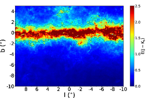
The biggest challenge to building an accurate map of the Bulge stellar density arises from the rapid extinction variations across different lines of sight. Following a similar approach to the one described in Gonzalez et al. (2011), we use the RC giants in the VVV to build a high resolution (1^′ x 1^′ sampling) reddening map (see Figure 1) by comparing the mean colour of the RC stars observed in each field with that of the RC population in Baade’s window, $(J^{\prime}-K^{\prime}_{s})_{\mathrm{BW}}=0.89$ (throughout the paper we denote with $J^{\prime}$ and $K^{\prime}_{s}$ the observed VVV magnitudes and with $J$ and $K_{s}$ the extinction-corrected magnitudes), under the assumption that the intrinsic colour of the RC remains, on average, the same across the Bulge i.e. $J-K_{s}=0.62$. We adopt the Nishiyama et al. (2009) interstellar extinction law derived for the central Bulge region since it was shown to reproduce most accurately the extinction of RC stars in the VVV (Gonzalez et al., 2012b).

To build the extinction map we combine the 2MASS-VVV colour transformations $J^{\prime}=J^{\prime}_{\mathrm{2M}}-0.065(J^{\prime}-K^{\prime}_{s})_{\mathrm{2M}}$ and $K^{\prime}_{s}=K^{\prime}_{s\mathrm{2M}}+0.010(J^{\prime}-K^{\prime}_{s})_{\mathrm{2M}}$ and obtain the Nishiyama et al. (2009) law for VVV photometry: $A_{J}=1.351E(J^{\prime}-K^{\prime}_{s})$ and $A_{Ks}=0.482E(J^{\prime}-K^{\prime}_{s})$. We then calculate the reddening $E(J^{\prime}-K^{\prime}_{s})_{\mathrm{RC}}$ by comparing the observed RC colour in each field with its known extinction-free value in Baade’s window, $J-K_{s}=0.62$. We are able to use this technique in all Bulge fields covered by the survey as VVV photometry reaches the RC even in fields close to the Galactic Plane. Correction for extinction then proceeds on a star by star basis interpolating between the nearest four extinction map values.

The problem with using two dimensional maps such as ours, is the assumption that the extinction arises mainly from foreground material while in reality the sources are intermixed with dust at a range of distances, rendering the use of 3D reddening maps necessary especially at low latitudes ($|b|<3^{\circ}$). To compare the accuracy of 2D versus 3D dust maps, Schultheis et al. (2014) used a large spectroscopic sample of stars from the Apache Point Observatory Galactic Evolution Experiment (APOGEE) towards the MW Bulge, to conclude that for sources at distances larger than $\sim$ 4 kpc from the Sun, 2D maps can be applied without significant systematic offset. Moreover, it was noticed that none of the existing 3D maps agrees with independent extinction calculations based the APOGEE spectra towards the MW Bulge. Their study suggests that there is still room for improvement in the construction of 3D dust maps and that they do not outperform 2D maps for distances larger than 4 kpc from the Sun.

Figure 1: Reddening map in the Bulge area covered by the VVV survey, sampled at 1^′ x 1^′ with an effective resolution of 2^′. Overlaid on the map are contours of constant reddening $E(J^{\prime}-K^{\prime}_{s})=1.5$ (thin gray line) and $E(J^{\prime}-K^{\prime}_{s})=1.0$ (thick gray line). The region inside the $E(J^{\prime}-K^{\prime}_{s})=1.0$ contour, where the high reddening can cause incompleteness issues, is omitted in the VVV data modelling procedure explained in Section 5.

4 Model ingredients

In this Section we describe the main ingredients of our model which consists of synthetic thin and thick discs and a purely analytic Bulge. The model takes into account the disc contribution to the observed luminosity function as a function of field of view and magnitude and therefore has an advantage over recent VVV studies which either fitted a polynomial background to the discs and RGB (from both Bulge and discs) populations (Wegg & Gerhard, 2013) or assumed a uniform disc contamination throughout the Bulge area (Valenti et al., 2016).

The disc populations are built with Galaxia (Sharma et al., 2011), a C++ code able to generate synthetic surveys of the Milky Way, implementing the Besancon Galaxy model (Robin et al., 2003).

4.1 Isochrones

We add to Galaxia a recent set of PARSEC isochrones in the VISTA photometric system (Bressan et al., 2012), built using the default parameters of the online Padova CMD interface (we used PARSEC v1.2S + COLIBRI PR16 , described in Marigo et al. 2017). For the table of isochrones we choose 177 age bins and 39 metallicity bins, within the parameters range used in Galaxia for a previous PARSEC release (Marigo et al., 2008).

VVV zero point measurements (section 2.2 in Rubele et al. 2012) found a constant offset between the VISTA system calibration and the Vegamag system of the stellar models of 0.021 mag and 0.001 mag for the $J$ and $K_{s}$ bands respectively. This offset was implemented in the PARSEC version we use.

4.2 The discs

Figure 2: Number density distribution of mock thin and thick disc stars generated with Galaxia, in Galactic coordinates. The contours delineate the region with high reddening (see Figure 1) that will be excluded from the fitting procedure described in Sections 5 and 6. The integrated number of stars outside the masked area is equal to the number of disc stars in the VVV found in this work ($=N_{1}^{-}+N_{2}^{-}$ for model $E$ in Table 3). This figure is obtained averaging several mock samples to minimise shot noise.

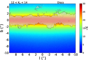
The thin and thick disc populations are an important component of the central regions; they are implemented by averaging several repeated mock catalogue realisations with Galaxia to minimise sampling noise. The disc models are shown in Figure 2, in Galactic coordinates - these are mock stars within the same range of extinction-corrected magnitudes and colours, $12<K_{s}<14$, $0.4<J-K_{s}<1.0$, used for the selected VVV sample (see Section 5). Overlaid we mark two contours of constant reddening $E(J^{\prime}-K^{\prime}_{s})=1.5$ (light gray) and $E(J^{\prime}-K^{\prime}_{s})=1.0$ (thick gray), as in Figure 1. The initial mass function (IMF), star formation rate (SFR), ages, metallicity and density laws of the discs implemented in $Galaxia$ are described in tables 1, 2 and 3 in Robin et al. (2003). The thin and thick discs are assumed to have a warp and a flare that is modelled following the prescription of Robin et al. (2003).

4.3 The Bulge luminosity function (LF)

4.3.1 Analytic description of the Bulge LF

We assume a 10 Gyrs old (Bruzual et al., 1997) Bulge population with solar metallicity [Fe/H]$=0$ dex (e.g. Zoccali et al., 2003) and a metallicity dispersion of $\sigma_{[Fe/H]}=0.4$ (Zoccali et al., 2008) with no metallicity gradients (default values of the Besancon Galaxy Model).

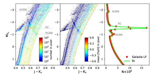
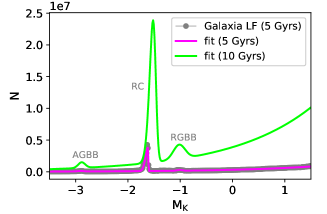
With these specifications, we simulate the LF with Galaxia using a Chabrier IMF, within the colour range $0.4<J-K_{s}<1.0$, adopted to reduce contamination from non-giants in the VVV data. The Chabrier IMF is chosen over the $Galaxia$ default Salpeter IMF as it was shown to describe more accurately observations and model predictions in the Galactic Bulge (see Chabrier 2003 and Portail et al. 2015 respectively). The resulting synthetic LF, $\phi_{B}(M_{K};$ 10 Gyrs), is shown in the third panel of Figure 3 in red. We model it following the description in section 3.1 of Nataf et al. (2015), with three Gaussians to represent the Asymptotic Giant Branch Bump (AGBB), the RC and the Red Giant Branch Bump (RGBB) and an exponential function for the Red Giant Branch (RGB) stars. The RC was modelled with either a Gaussian or a skew-Gaussian distribution, with the latter providing a slightly better fit; the addition of the skewness parameter affects only the $\mu^{\mathrm{RC}}$ and $\sigma^{\mathrm{RC}}$ values, as expected (see the results in Table 1). The only constraint was on the mean RGBB magnitude, set to $\mu^{\mathrm{RGBB}}=-1.02$, where the peak of the LF lies in the RGBB region. The fitted LF, with a skew-Gaussian model for the RC, is shown in green in the third panel of Figure 3, overlapping the histogrammed LF simulated with Galaxia (in red). We find $\mu^{\mathrm{RC}}=-1.53$, consistent with previous determinations of the mean RC magnitude in the K band (see table 1 in the RC review paper by Girardi 2016).

The first panel of the Figure shows the number density distribution of the Galaxia generated stars in a colour magnitude diagram with the specifications mentioned above, and the second panel the mean metallicity in each of those pixels. Notice the theoretical models predict the AGBB, RC and RGBB mean magnitudes depend on metallicity; this variation is responsible for the magnitude dispersions in the mock LF. The dependence of the RC magnitude on the age and metallicity of the population has also been recorded empirically, e.g. the globular cluster 47 Tuc (age $=11$ Gyrs, [Fe/H] $=$-0.7 dex) has $\mu_{K}^{\mathrm{RC}}=-1.28$ mag while the much younger open cluster NGC 2204 (age = $1.7$ Gyrs, [Fe/H] $=$ -0.38 dex) has $\mu_{K}^{\mathrm{RC}}=-1.67$ (see table 1 in Percival & Salaris 2003 and top panel of figure 6 inGirardi 2016 which shows the RC in open clusters as a function of age and metallicity). It is therefore important, for building a reliable LF, to have accurate assumptions on the metallicity distribution function and the age of the Bulge population as they influences both the mean magnitude of each Gaussian (AGBB/RC/RGBB) and the magnitude dispersion.

The photometric metallicity maps derived by Gonzalez et al. (2013) measure a metallicity gradient in the Bulge of $\sim$0.04 dex/deg. The metal rich stars ([Fe/H] $\sim$ 0) dominate the inner regions with little to no metallicity gradient within $|b|<5^{\circ}$, while more metal poor stars prevail at distances further from the plane. The absolute majority of stars in the VVV survey are found at $|b|<5^{\circ}$, so our assumption of solar metallicity (adopted by Robin et al. 2003 and after, by Wegg & Gerhard 2013) with 0.4 dex dispersion should be a good approximation. Recent measurements have also shown that the metallicity distribution function of RC stars is bimodal (e.g. Zoccali et al., 2017) with two peaks, one slightly more metal rich and one less metal rich than the Sun; however the two mean metallicities and their ratio vary across the 26 sparse fields observed by the GIRAFFE survey (see figure 4 in Zoccali et al. 2017), making it difficult to implement these variations in a spatially varying LF over 315 square degrees.

An age variation in the Bulge stellar population is another factor that could shift the mean magnitude and increase the magnitude dispersion $\sigma$ of the RC, AGBB and RGBB populations: for example, according to theoretical models, the RC of a 5 Gyrs population is 0.1 mag brighter than that of a 10 Gyrs population (see the violet LF in the right panel of Figure 3 and the last row of Table 1 which gives the model parameters with a skew-Gaussian RC distribution). In literature there is overall good consensus on the age (10 Gyrs) of the Bulge (see review by Zoccali & Valenti 2016 and references therein), with some studies postulating the existence of a younger Bulge component (e.g. Ness et al., 2014; Catchpole et al., 2016; Haywood et al., 2016).

In the next subsection we take into account other factors, such as the extinction residuals and the VVV photometric errors, that influence the magnitude dispersion of the RC, RGBB and AGBB (more often we just mention $\sigma^{\mathrm{RC}}$, as the RC is the main population in our VVV sample), which are characteristic to the survey and our methods -rather than to the intrinsic Bulge population. The LF is further discussed in Section 7.

Figure 3: $First$ $panel$: Number density distribution of Galaxia generated stars using PARSEC isochrones in a colour magnitude diagram with [Fe/H] = 0 dex, $\sigma_{[Fe/H]}=0.4$ and age $=10$ Gyrs. $Second$ $panel:$ mean metallicity in each of the pixels in the first panel. $Third$ $panel$: Galaxia synthetic LF (red) and model (green) with 3 Gaussians and an exponential, following the Nataf et al. (2015) description (the parameters are given in the top row of Table 1). $Fourth$ $panel$: Model LF for a 5 Gyrs old (purple) and a 10 Gyrs old (green) population. The RC of 5 Gyrs old population is 0.1 mag brighter than the RC of the 10 Gyrs old population. The integrated area under each curve gives the total number of stars we found for each component in the results section (see the $N_{3}$ values in Table 3 for components $S$ and $E$, in model $S+E$)

.

Table 1: Parameters describing the Galaxia generated synthetic LF modelled with three Gaussians to represent the RC, AGBB and RGBB and an exponential function for the RGB (see equation in section 3.1 of Nataf et al. 2015 and the caption of Figure 3). For a 10 Gyrs old population (age in the first column), we provide the parameters for both a skew-Gaussian and a Gaussian RC distribution, in the first and second row respectively. The parameters for a 5 Gyrs population, where the RC is modelled with skew-Gaussian distribution, are given in the bottom row.

age	$a$	$b$	$(f^{\mathrm{AGBB}},\mu^{\mathrm{AGBB}},\sigma^{\mathrm{AGBB}})$	$(f^{\mathrm{RC}},\mu^{\mathrm{RC}},\sigma^{\mathrm{RC}},\gamma^{\mathrm{RC}})$	$(f^{\mathrm{RGBB}},\mu^{\mathrm{RGBB}},\sigma^{\mathrm{RGBB}})$
10	0.199	0.642	0.0077 ,-2.886, 0.067	0.174, -1.472, 0.091, -2.1	0.032, -1.02, 0.112
$\pm$	0.003	0.012	0.0030, 0.029, 0.029	0.003, 0.002, 0.003, 0.2	0.004, fixed, 0.015
10	0.198	0.642	0.0077 , -2.886, 0.068	0.174, -1.528, 0.062, —	0.032, -1.02, 0.108
$\pm$	0.004	0.017	0.0031, 0.031, 0.031	0.003, 0.002, 0.001,—	0.004, fixed, 0.016
5	0.204	0.653	0.0076 ,-2.908, 0.055	0.166, -1.610, 0.052, -9.8	0.011, -1.018, 0.050
$\pm$	0.003	0.013	0.0023, 0.019, 0.019	0.002, 0.003, 0.001, -0.9	0.002, 0.011, 0.011

Figure 4: Magnitude dispersion of the LF in the $K_{s}$ band, $\sigma_{K_{s}}(l,b)$, due to VISTA photometric errors and residual extinction. The dispersion is dominated by residuals in the extinction and its distribution follows closely the reddening map. The photometric errors increase up to $\sigma_{K_{s}}^{\mathrm{phot}}\sim 0.03$ in the very central region. The vertical stripes in correspondence with the edges of the tiles are caused by known issues with one of the VISTA detectors (#16).

4.3.2 VISTA photometric errors and residual extinction

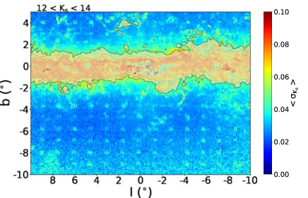
The observed RC in the VVV colour-magnitude diagram (CMD), shown in Figure 7, will be more spread compared to the theoretical LF because of variations in distance, extinction, age and metallicity in the Bulge population, coupled with survey specific photometric errors. We calculate the total magnitude dispersion $\sigma_{K_{s}}(l,b)$ caused by photometric errors and extinction corrections (see equation 6 in Wegg & Gerhard 2013) and show its spatial variation in Galactic coordinates in Figure 4. To account for the effects of photometric errors and residual extinction correction we convolve the theoretical LF (green curve in Figure 3) with a Gaussian kernel with $\sigma_{K_{s}}(l,b)$, for models $E$ and $S$ described in the next session. However, the effects of the convolution are negligible on the number of counts predicted by our model: convolving the intrinsic LF with a Gaussian with the maximum dispersion, max($\sigma_{K_{s}}(l,b))=0.065$, found close to the exclusion boundary $E(J^{\prime}-K^{\prime}_{s})$ = 0.1, causes a variation in the peak of the observed magnitude distribution $N(K_{s})$ smaller than 1.8%. As the convolution slows down our fitting procedure and has negligible effects, it will not be performed for models with two components and the tests in the next sections.

Figure 5: X-Y star number density map for the Bulge mock catalogue generated by Galaxia with $-5^{\circ}<b<5^{\circ}$. This realisation has a $G$ model (Equation 1) density law, with [$x_{0}$,$y_{0}$, $z_{0}$, $|\alpha|$] = [1.6, 0.4, 0.4, 20^∘] and cut-off radius, $R_{c}=$ 2.5 kpc (red circle). Notice that for a very long bar (large values of $x_{0}$), the near end would be cut off by the limiting longitude of the VVV survey $l=10^{\circ}$, preventing us to estimate the correct extent of the semi-major axis. The angle between the major axis direction and the Sun-Galactic centre direction gives rise to a longitudinal asymmetry in the $(l,b)$ density distributions.

4.4 The Bulge density distribution

Several earlier Bulge studies have shown that the distribution of sources in the Bulge is triaxial, while Dwek et al. (1995) found that Gaussian-like functions provide a better fit to the COBE/DIRBE observations of the Bulge projected surface brightness at 2.2 $\mu$m rather than other classes of functions. In particular, they showed that a ‘boxy’ Gaussian,

$$\rho_{B}=\rho_{0}\mathrm{exp}^{-0.5r_{s}^{2}}\qquad(\mathrm{model}\quad G)$$ (1)

where,

$$r_{s}^{2}=\sqrt{\bigg{[}\bigg{(}\frac{X}{x_{0}}\bigg{)}^{2}+\bigg{(}\frac{Y}{y_{0}}\bigg{)}^{2}\bigg{]}^{2}+\bigg{(}\frac{Z}{z_{0}}\bigg{)}^{4}}\quad,$$

best described their data and this is the model adopted by Robin et al. (2003) for the Besancon Galaxy model which is incorporated in the Galaxia code.

In the next section, we fit the data with a more general form of Equation 1, namely an exponential-type model (model E), with 7 free parameters, including the viewing angle, $\alpha$:

$$\rho_{B}=\rho_{0}\mathrm{exp}^{-0.5r_{s}^{n}}\qquad(\mathrm{model}\quad E)$$ (2)

where,

$$r_{s}^{c_{\|}}=\bigg{[}\bigg{(}\frac{X}{x_{0}}\bigg{)}^{c_{\perp}}+\bigg{(}\frac{Y}{y_{0}}\bigg{)}^{c_{\perp}}\bigg{]}^{\frac{c_{\|}}{c_{\perp}}}+\bigg{(}\frac{Z}{z_{0}}\bigg{)}^{c_{\|}}\quad.$$

Freudenreich (1998) preferred a hyperbolic secant density distribution

$$\rho_{B}=\mathrm{sech}^{2}(r_{s})\qquad(\mathrm{model}\quad S)$$ (3)

to the exponential-type model, which has the advantage of having one parameter less, the power $n$. This function will also be used to fit the Bulge density distribution.

The free parameters of the Bulge model, are:

• $\alpha$, the angle between the Bulge major axis and the line connecting the Sun to the Galactic Centre; we fix equal to 0 the angles $\beta$, the tilt angle between the Bulge plane and the Galactic plane and $\gamma$, the roll angle around the Bulge major axis ;

• $x_{0}$, the scale-length on the major axis, and $y_{0}$ and $z_{0}$ the scale lengths on the in-plane and off-plane minor axes;

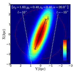
• $c_{\perp}$ and $c_{||}$, the face-on and edge-on shape parameters: the Bulge has an in-plane elliptical shape when $c_{\perp}=$2 (see Figure 5), diamond shape when $c_{\perp}<2$ and boxy shape when $c_{\perp}>2$;

• the power $n$;

$\rho_{0}$ is the density normalisation and $R_{c}$ is a cutoff radius, kept fixed during the fitting procedure. The cutoff radius, $R_{c}$, is implemented by multiplying the density distribution $\rho_{B}$ by the tapering function

$$f(R)=1\qquad\quad\quad\mathrm{if}\quad R<R_{c}$$

$$=\mathrm{exp}^{-2(R-R_{c})^{2}}\quad\mathrm{if}\quad R>R_{c}$$

to produce a smooth transition to zero for the source number density beyond $R_{c}$ (also used for the Bulge density law in Sharma et al. 2011, see their table 1).

We do not attempt to build a parametric model of the Bulge X-shape, which we discuss in detail in Section 7.

4.5 Other stellar populations in the inner MW

We assume the halo population contributes a negligible fraction of RC stars to the whole VVV RC sample (see e.g. column 4 of table 3 in Zoccali et al. 2017). Our colour magnitude selection box does not include stars with $J-K_{s}<0.4$ mag, where we would expect to see the halo old metal poor stars. We also assume that the ring, the spiral arms and the thin long bar (e.g. González-Fernández et al., 2014; Wegg et al., 2015) do not significantly contribute to the VVV star counts in the fields selected for the analysis (regions of low reddening, with $E(J^{\prime}-K^{\prime}_{s})<$1.0) as they are confined to the Galactic Plane.

We therefore assume that in the regions probed by our analysis, the thin disc, thick disc and the Bulge make up the bulk of the stellar density and the contribution of other populations is negligible.

5 The fitting procedure. Test on mock data

In this section we outline the fitting procedure and demonstrate its robustness by testing it on a mock Bulge dataset generated with Galaxia pre-defined parameters. These tests help assess the quality of our results when fitting the VVV dataset in Section 6.

5.1 The mock data

The mock data ($D^{\mathrm{mock}}$) is a catalogue of stars generated with Galaxia (Sharma et al., 2011) using a specified set of parameters. It consists of a synthetic disc ($N_{d}^{\mathrm{mock}}$) multiplied by a constant ($Scale$) and a mock sample of Bulge/Bar stars ($N_{B}^{mock}$) so that the number of stars in a given sightline at a given magnitude $K_{s}$ is $D^{\mathrm{mock}}=N_{d}^{\mathrm{mock}}\times Scale+N_{B}^{\mathrm{mock}}$, where $Scale=0.4$ (a value close to the observed value reported in Table 3). The parameter $Scale$, introduced to match the total number of disc stars, is a free parameter in our model and is needed to account for variations in the number density introduced by changing the isochrones set. We generate with Galaxia a mock Bulge catalogue of $\sim$13 million stars, to roughly match the number of VVV stars, following model $G$ (Equation 1) density distribution with parameters [$x_{0}$, $y_{0}$, $z_{0}$, $|\alpha|$] = [1.6, 0.4, 0.4, 20^∘]. This distribution is shown in Figure 5, projected onto the XY-plane, where the Galactic Centre is at [$X,Y$] = [0,0]. Only the latitude range $-5^{\circ}<b<5^{\circ}$ is plotted but we fit $-10^{\circ}<b<5^{\circ}$, as in the data.

Figure 6: Slices of $\ln$($\chi_{red}^{2}$) maps as a function of two varying parameters while the other three are fixed to their true value. The absolute minimum found by the grid search (darkest violet bin) and the 10 BFGS runs (red open circle) coincides with the true value (yellow circle). The BFGS runs were initialised in random points (full red circles) covering the full parameter space.

5.2 The model

The model ($M$) predicting the number of stars in a given line of sight at a given magnitude, has the general form:

$$M=<N_{d}>\times Scale+N_{\mathrm{B}}$$ (4)

where $<N_{d}>$ is an average over several $N_{d}$ disc realisations (see Figure 2). We calculate $N_{\mathrm{B}}$, the Bulge apparent magnitude distribution, analytically. For each field with Galactic coordinates $(l,b)_{i}$, d$N_{\mathrm{B}}(K_{s})=N_{\mathrm{B}}(K_{s})$d$K_{s}$ is the differential star counts with apparent magnitudes in the range ($K_{s}$, $K_{s}+dK_{s}$)

$$\begin{split}\mathrm{d}N_{\mathrm{B}}(K_{s})=\rho_{\mathrm{B}}(D)\phi_{\mathrm{B}}(M_{K_{s}})D^{2}\cos(b)\Delta l\Delta b\mathrm{d}D,\end{split}$$

where the absolute magnitude is a function of the apparent magnitude and distance modulus $M_{K_{s}}=K_{s}-5\log_{10}D+5$. $N_{B}(K_{s})$, the apparent magnitude distribution, in a given direction $(l,b)_{i}$ (and a solid angle $\Omega$) is the integral of the LF $\phi_{\mathrm{B}}$ times the density law $\rho_{\mathrm{B}}(D)$

$$N_{\mathrm{B}}(K_{s})=\int_{4}^{12}\rho_{\mathrm{B}}(D)\phi_{B}(K_{s}-5\log_{10}D+5)D^{2}\Omega\mathrm{d}D.$$ (5)

In the fitting process, we calculate the predicted number of counts $N_{\mathrm{B}}(K_{s})$ for 20 different values of $K_{s}$ between $12<K_{s}/$mag$<14$ so that the total number of counts is $N_{\mathrm{B}}(12<K_{s}<14)=N_{\mathrm{B}}=\sum\limits_{j=0}^{20}(N_{\mathrm{B}})_{j}(K_{s})$. The limits of the integral in Equation 5 are set to 4 and 12 kpc as $\rho_{\mathrm{B}}$ approaches zero outside this range for $12<K_{s}<14$.

5.3 The fitting procedure

5.3.1 Method

We follow a Bayesian approach which requires us to define the likelihood function of our data and the prior distributions of the parameters $\vartheta$. The likelihood of the entire data set, $L$, is the product of the probability of each number count $N_{i}$ in the $n_{\mathrm{fov}}$ fields of view $(l,b)_{i}$, given our model prediction $M$ (Equation 4):

$$L=\prod\limits_{i=1}^{n_{\mathrm{fov}}}\mathrm{p}(N_{i}|M(\vartheta))\quad.$$

Assuming the measurements $N_{i}$ follow a Poisson distribution we search for the parameters $\vartheta$ that maximise the logarithm of the likelihood for the whole data set:

$$\mathrm{ln}L=\sum\limits_{i=1}^{n_{\mathrm{fov}}}[N_{i}\mathrm{ln}M_{i}(\vartheta)-M_{i}(\vartheta)]+\mathrm{constant}$$ (6)

Table 2: Best fit results for the mock catalogue generated with Galaxia. The first column specifies the model, the second column the shape of the density distribution, the third column the reduced chi squared $\tilde{\chi}^{2}$ as an indication of the ’goodness’ of the fit, the fourth column the log-likelihood, the fifth column the best fit parameters of the density distribution and finally, the sixth column, gives the discs scaling, $Scale$. In the last two rows we list the results obtained from fitting an $S$ model and an exponential form of the density distribution, where $r$ is the Galactocentric radius. From the comparison of the results, we can conclude that the errors on the parameters will be dominated by systematics.

				Test Galaxia
	$\rho_{b}$	$\tilde{\chi}^{2}$	-ln($L_{G}$)	[$x_{0}$, $y_{0}$,$z_{0}$, $\alpha$, $c_{//}$, $c_{\perp}$,$n$]	$Scale$
$Galaxia$ model	$\propto\mathrm{exp}^{-0.5r_{s}^{2}}$	-	-	[1.600, 0.400, 0.400, -20.00, 4.000, 2.000, 2.000]	0.400
fitted model	$\propto\mathrm{exp}^{-0.5r_{s}^{n}}$	1.00	384,408	[1.629, 0.403, 0.400, -20.01, 3.877, 1.923, 1.993]	0.386
fitted model	$\propto$ sech${}^{2}(r_{s})$	1.15	416,195	[1.834, 0.456, 0.429, -19.79, 3.279, 1.717, -]	0.271
fitted model	$\propto\mathrm{exp}^{-0.5r^{2}}$	1.10	406,338	[1.961, 0.468, 0.454, -20.30, -, -, -]	0.317

We use the $Python$ implemented limited-memory BFGS method (L-BFGS, Byrd et al., 1995) that calculates an estimate of the inverse Hessian matrix to facilitate search through the model parameter space. This method is particularly well suited for optimisation problems with a large number of parameters, e.g. including the ones governing the shape of the Bulge density, $n$, $c_{\perp}$, $c_{||}$. Moreover, it allows the user to constrain the parameters within reasonable physical values, equivalent to adopting a uniform Bayesian prior. We draw the initial (guess) values of the free parameters from uniform distributions, with the same limits as our grid search, and add three extra parameters, $n$, $c_{\perp}$, $c_{||}$, also drawn from random uniform distributions, with limits as in Figure 6.

5.3.2 Optimal integration step estimation

Before fitting, we need to find the most appropriate integration steps ($\Delta l,\Delta b$ and $\Delta D$) for the Bulge model ($N_{B}$), the only population we generate analytically and whose parameters we want to determine. Using the same density function and true values in both the synthetic Bulge and the mock catalogue, we made several tests varying ($\Delta l,\Delta b$ and $\Delta D$) in our model to find the resolution that produces the best match to the mock catalogue. We found that small-size fields ($\Delta$$l$, $\Delta$$b$) = (0.1^∘,0.1^∘) produced a reduced chi-squared $\tilde{\chi}^{2}$ $\approx$ 1 while the distance step can be relatively large (e.g. $400$ pc) given that we calculate $N_{B}(K_{s})$ for magnitude step sizes of $dK_{s}=0.1$ mag. With this choice, the model gave a perfect match to the mock catalogue, with a reduced chi-squared of $\tilde{\chi}^{2}=1.02$. The number of sources varies rapidly from pencil beam to pencil beam in the inner Galaxy, so it is not surprising that in order to have an accurate model prediction, we need to calculate parameters over a very fine grid of Galactic coordinates.

To fit the VVV data we increase the magnitude resolution to $\mathrm{d}K_{s}=0.05$ mag, for which we need to employ a finer distance integration step of $\Delta D=50$ pc.

5.4 Test results

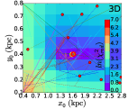
In the test run we compute chi-squared maps varying five parameters $\vartheta_{0}=$ [$x_{0}$,$y_{0}$, $z_{0}$, $|\alpha|$,S], over a wide range of values on a coarse grid [$\Delta x_{0}$,$\Delta y_{0}$, $\Delta z_{0}$, $\Delta|\alpha|$, $\Delta S$] = [0.3 kpc, 0.1 kpc, 0.1 kpc, 2^∘, 0.2 ]. The high reddening region where $E(J^{\prime}-K^{\prime}_{s})>1.0$ (gray mask in Figure 4) is excluded from the test, to reproduce the data fitting procedure. We compute $N_{B}(12<K_{s}<14)$ for fields of 0.1${}^{\circ}\times$ 0.1^∘ and in each pencil beam we calculate $N_{B}$ for 20 values of magnitude $K_{s}$ (Equation 5). We group the model $M$ (Equation 4) in 5 magnitude bins to be fitted on 5 magnitudes bins in the mock catalogue (VVV data in Section 6), in order to extract information about the depth distribution of sources in the Bulge.

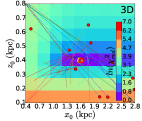
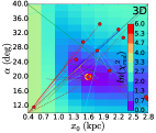
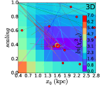
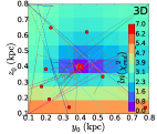
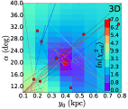
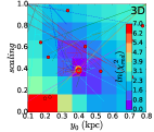
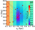
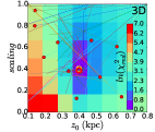
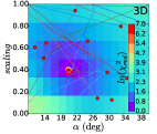
Figure 6 shows the resulting slices of $\ln(\chi^{2})$ maps as a function of the two varying parameters, while the other three are fixed to their true value. The absolute minima (violet bin in the figure) coincide with the true values used as an input of the model (yellow open circles in the figure), proving that the method works well. These maps also reveal the correlations between parameters, see e.g. $\alpha$ versus $x_{0}$.

The mock catalogue can also be used to test the accuracy of the L-BFGS method employed in Section 6 to find the parameters of the real Bulge density distribution. The 10 filled red circles in Figure 6 are the initial parameters of 10 L-BFGS independent runs with initial values drawn from uniform distributions. The identical final solutions of each run (red open circles) where the algorithm converges, coincide with the fiducial value (yellow circles) $\vartheta=$[1.629, 0.4026, 0.3996, 20.01, 3.88,1.925,1.993,0.3865] $\pm$ [0.004, 0.0009, 0.0009, 0.02, 0.015, 0.007, 0.004, 0.0009] and are very close to the true value $\vartheta_{0}=[1.6,0.4,0.4,20,4,2,2,0.4]$, included in Table 2. The statistical errors in the parameters, obtained from the covariance matrix, are extremely small and we consider them to be negligible in comparison to the systematic errors (see Section 7). However, the test on the mock data also provides an indication of how well the fitting method recovers the true parameters of the Bulge density distribution (see the first two lines in Table 2, which shows the true values and the best fit values found using the L-BFGS minimisation method). The agreement here leads us to conclude that the random error component is well-captured by the method.

An estimate of the systematic errors can be obtained by adopting different density distributions in the models as compared to the mock data. In Table 2 we list the results obtained from fitting a hyperbolic secant model and an exponential form of the density distribution, with $r$ the Galactocentric radius (last two rows of the table) and from comparing the results of the three fits to the true values $\vartheta_{0}$, we notice that the best fit parameters $\vartheta$ of the correct density law are close to their true value $\vartheta_{0}$ ( $\delta\vartheta=[x,y,z]-[x_{0},y_{0},z_{0}]=[0.029,0.003,0.000]$) while when fitting the ‘wrong’ density laws, the results diverge significantly from the true value ($\delta\vartheta=[0.234,0.056,0.029]$ and $\delta\vartheta=[0.361,0.068,0.054]$ for the two ‘wrong’ models). In conclusion, the choice of the density distribution alone introduces systematic errors much larger than the standard errors.

6 Fitting the VVV data

Figure 7: CMD of all the Bulge VVV targets with class K $<0$ and $E(J^{\prime}-K^{\prime}_{s})<1.0$, totalling $\sim$ 96$\times 10^{6}$ sources, both before ($left$ $panel$) and after ($right$ $panel$) correcting for reddening (shown in Figure 1). The red square marks our working sample colour - magnitude selection (their spatial distribution shown in Figure 8). The dotted white lines show the five magnitude slices used for the plots in Figures 10 and 11. The spatial distribution of the stars in each slice is shown in the left panels of Figure 10.

Figure 8: The number density distribution of VVV stars with $12<K_{s}$/mag$<14$ and $0.4<J-K_{s}<1.0$ (red selection box in Figure 7), in Galactic coordinates. The contours delineate the highly reddened regions $E(J^{\prime}-K^{\prime}_{s})=1.5$ (light gray) and $E(J^{\prime}-K^{\prime}_{s})=1.0$ (thick gray). Close to the Galactic Plane (e.g. inside the $E(J^{\prime}-K^{\prime}_{s})=1.0$ reddening contour) the dust causes incompleteness issues. Notice also the variation in the number of counts in adjacent tiles in the inner regions.

In this section we fit a triaxial density model to the observed VVV magnitude distribution in the RC region of the colour-magnitude diagram. We focus on describing the inner Milky Way large scale structure by finding a model capable of reproducing the distributions seen in the majority of the fields at the expense of discrepancy in a small number of fields, which include fields close to the Galactic Plane/Centre and those at $b<-5^{\circ}$, where a double RC is observed (e.g. McWilliam & Zoccali, 2010; Saito et al., 2012).

6.1 Data sample

The photometry of every source in the single band tile catalogues produced by CASU is labelled with a morphological classification flag. In the following sections, we use detections classified as ‘stellar’, ‘borderline stellar’ or ‘saturated stars’ in the $K_{s}$ magnitude band, which has the best seeing. We avoid applying a strict cleaning procedure in order to work with a sample of Bulge stars as complete as possible.

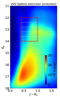
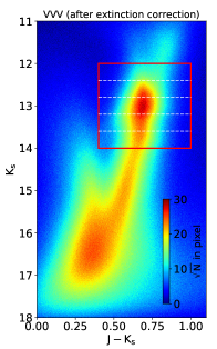
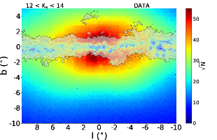
We choose sources with photometric errors $\sigma_{J}$, $\sigma_{K_{s}}<0.2$ mag and colours $(J-K_{s})>0.4$, to minimise contamination from disc Main Sequence stars and $(J-K_{s})<1.0$ to separate Red Giant stars from spurious objects and highly reddened K and M dwarfs. In our analysis, we apply a faint end magnitude cut of $K_{s}=14$ mag, which we consider adequate to minimise the effects of incompleteness given the substantial extinction over the field-of-view, and a bright end limit of $K_{s}=12$ mag to avoid saturation and non-linearity (Gonzalez et al., 2013) which sets in around $K^{\prime}_{s}<11.5$. These cuts form our colour-magnitude selection for the VVV working sample and are marked with a red box in Figure 7. The two panels show the distribution of all the VVV sources with $E(J^{\prime}-K^{\prime}_{s})<1$, totalling 96 milion objects, in a CMD before (left panel) and after (right panel) extinction correction. The observed $K_{s}^{{}^{\prime}}$-band magnitudes for each star are corrected for the effects of extinction, $K_{s}=K_{s}^{{}^{\prime}}-A_{K_{s}}(l,b)$, using the reddening maps $E(J^{\prime}-K^{\prime}_{s})$ constructed from the VVV data (see Section 3). In the left panel, most of the RC stars are outside our selection box due to extinction and reddening effects which cause the stars to appear fainter and cooler. The number density distribution of all the stars within the red selection box is then shown in Galactic coordinates in Figure 8. Again, the contours delineate the highly reddened regions $E(J^{\prime}-K^{\prime}_{s})=1.5$ (light gray) and $E(J^{\prime}-K^{\prime}_{s})=1.0$ (thick gray).

We illustrate the completeness of the survey by plotting the variation of the observed magnitude distributions with latitude in Figure 19 of the Appendix, both before (top row) and after (bottom row) extinction correction. The stars were selected in $1.0^{\circ}$ x $0.4^{\circ}$ fields at constant longitude $l=0^{\circ}$ and decreasing latitude $b$. The fields within the $E(J^{\prime}-K^{\prime}_{s})=1$ mag contour are incomplete with the high extinction causing a depletion of stars in the 13 to 15 $K^{\prime}_{s}$ magnitude range and a rapid drop in the star counts for $K^{\prime}_{s}>15$ mag (see orange dotted line in the figure). However, further from the plane, the incompleteness limit increases and at $b\sim-3^{\circ}$ the distribution is complete up to $K^{\prime}_{s}\sim 15.2$ or $K_{s}\sim 15$, making our working magnitude range (red vertical lines in the figure) a fairly conservative cut.

6.2 An example data fit

Figure 9: Apparent magnitude distributions for the data (red) and a global best fit model, $M=<N_{d}>\times Scale+N_{B}$ (green triangles). The apparent magnitude distribution $N_{\mathrm{B}}$ of the Bulge (dark green, Equation 5) is a convolution between the absolute magnitude LF (green, labeled ‘LF+14.5’, where 14.5 is the distance modulus added to the absolute magnitudes $M_{K_{s}}$) and the density law $\rho_{B}(l,b,D)$ (dotted dark green, Equation 2). The discs $<N_{d}>\times Scale$ (labeled ‘DISCS’) are shown in gray.

Figure 10: Data number density distribution ($left$ $panels$) and best fit models $E$ ($middle$) and $(S+E)$ ($right$) in Galactic coordinates. The 5 rows are slices of $K_{s}$ magnitudes between $12<K_{s}<14$ with the brightest magnitude slice on the top row. High extinction causes incompleteness close to the Galactic plane as it can be seen in the data, therefore the region within the $E(J^{\prime}-K^{\prime}_{s})=1.0$ contour (thick gray) was excluded from all analysis. The fitted model appears good in nearly all regions (see discussion in Section 6.5); the residuals between the data and each model are shown Figure 11.

Figure 11: Left panels: component $E$ of the $(S+E)$ model with axis ratio [1:0.14:0.17] and viewing angle $|\alpha|=1^{\circ}$. Middle panels: differences between data and model $E$, divided by the Poisson noise in the model. The model does not perform well in the central regions, $|l|<2^{\circ}$ and $|b|<3^{\circ}$, where an excess is visible in the data, especially in the brightest magnitude bins (see the discussion in Section 7.4). Right panels: same as in the middle panels but for model $(S+E)$. The addition of the extra component (shown in the left panels) improves the quality of the fit in the inner regions. The magnitude distributions in the $2^{\circ}\times 1^{\circ}$ fields marked with either letters or crosses, are provided in Figures 14 and 15 respectively. We mark in yellow the fields with $b<-5^{\circ}$ for which we show the López-Corredoira (2017) X-shaped model in the same figures.

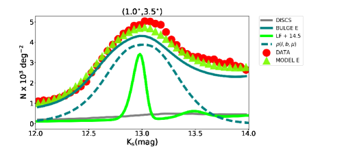
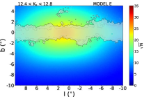
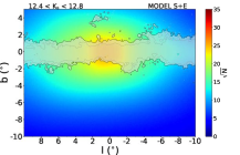
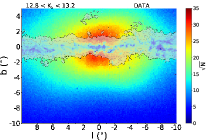
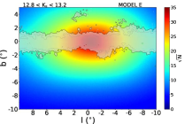
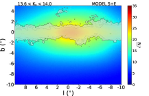
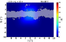
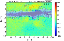
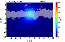
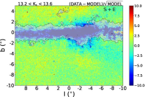
The functions involved in the data fitting procedure are illustrated in Figure 9. The apparent magnitude distribution $N_{\mathrm{B}}$ of the Bulge (thick blue, Equation 5) is the integral of the absolute magnitude LF (green, labeled ‘LF+14.5’) with a distance modulus of 14.5 added to the absolute magnitudes, $M_{K_{s}}$, times the density law $\rho_{\mathrm{B}}(l,b,D)$ (in the figure we show $\rho_{\mathrm{B}}(l,b,\mu)$ in magenta, Equation 2). The total apparent magnitude distribution $M=<N_{\mathrm{d}}>\times Scale+N_{\mathrm{B}}$ (thin dotted line, labeled ‘MODEL E’) is given by the sum of the Bulge $N_{\mathrm{B}}$ (labeled Bulge E) and the discs $<N_{\mathrm{d}}>$ (labeled ‘DISCS’). To obtain $N_{B}$ (thick blue line), Equation 5 was calculated on a grid of 20 x 10 $(l,b)_{i}$ fields of view between $0^{\circ}<l<2^{\circ}$ and $3^{\circ}<b<4^{\circ}$ for 50 $K_{s}$ apparent magnitudes bins between $12<K_{s}<14$ mag.

We do not fit directly for the Sun-Galactic centre distance, which is a fixed parameter, $R_{\sun}=8$ kpc (see table 1 in Vallée 2017), but we allow the mean magnitude of the RC to vary by $\Delta\mu^{\mathrm{RC}}$. Here $\Delta\mu^{\mathrm{RC}}$ can translate to a new value for $R_{\sun}$, as it is effectively a distance modulus shift, or a new value for the mean magnitude of the RC. For all models we found $\Delta\mu^{\mathrm{RC}}=-0.1$, or $\mu_{10}^{\mathrm{RC}}=-1.63$ at $R_{\sun}=8$ kpc, similar to Laney et al. 2012 and Hawkins et al. 2017 who found $M_{K}^{\mathrm{RC}}=-1.61$ using nearby Hipparcos and Gaia stars respectively, and Wegg et al. 2015 who found $M_{K}^{\mathrm{RC}}=-1.67$ at $R_{\odot}=$8 kpc (note their LF were constructed interpolating the BASTI isochrones in the 2MASS photometric system, Pietrinferni et al. 2004).

The model plotted in Figure 9 is a result of the full global fit of the whole VVV dataset, discussed in the next subsection. We performed the fits for two cut-off radii, $R_{\mathrm{c}}=$2.5 and 4.5 kpc and found that $R_{\mathrm{c}}=4.5$ kpc provides a better fit, therefore in the remainder of this work it is kept constant.

6.3 The full Bulge sample fit

We compute the model on a continuous grid of 6${}^{\prime}\times 6^{\prime}$ fields covering the whole area of the VVV survey amounting to 200 $\times$ 150 $(l,b)_{i}$ lines of sight, for 40 magnitude bins $K_{s}$ (green triangles in Figure 9) to be fitted to the data (red circles in the same figure). We first consider a single Bulge population and next, we add a second component to improve the agreement in the central regions at low latitudes where the residuals highlight an overdensity.

The three models we consider are:

• model $E$: the density model is described by an exponential-type model (Equation 2) and has a 10 Gyr-old input LF (see Figure 3). The model $M$ has 10 free parameters, 7 describing the density law, a scaling for the thin discs and one for the thick disc and the RC peak magnitude shift $\Delta\mu^{\mathrm{RC}}$;

• model $S$: this density law is described by a hyperbolic secant density distribution (Equation 3) and has a 10 Gyr-old input luminosity function, the same as model $E$. The model has 9 free parameters, 6 describing the density law, a scaling factor for the thin discs and one for the thick disc and $\Delta\mu^{\mathrm{RC}}$;

• model $S+E$: Robin et al. (2012) using 2MASS data found that a combination of an exponential-tye ($E$) and a sech² ($S$) density law provide the best description of the Bulge (see their table 2) and we use the same description for the VVV data. In total, the model has 16 free parameters, 7 for model $E$, 6 for model $S$, two scaling factor for the discs and one for the ratio between the two Bulge components. The magnitude shift is not a free parameter, we set to $\Delta_{\mu}^{\mathrm{RC}}=-0.1$ in accordance with the results found in the single component fit.

We perform several runs of the L-BFGS minimisation starting from random initial points to test whether the final result is dependent on the initialisation position and to avoid being trapped in a local minimum. We consider our best solution to be the one that maximises the log-likelihood, (Equation 6) across all trials; note that several runs may actually converge to the same best-fit solution. We do not have tight constrains on the parameters, limiting them to an initial set of random values that would have a physical meaning as described in the previous section. The model $(S+E)$ has 16 free parameters so to avoid getting not meaningful results we choose the starting point for the main component S to be the best fit solution of the one population fit (model $S$), while the starting point for the E component is drawn from a uniform random distribution.

Table 3: Best fit results for the three density models we have used to reproduce the VVV data. The $first$ $column$ assigns a label for each result, for easier reference in the text; the $second$ $column$ specifies the model $S$, $E$ or $S+E$; $third$ $column$ the logarithm of the likelihood, which is an indication of the ‘goodness’ of the fit. The $fourth$ $column$ lists three values: the $\Delta_{\mu}^{\mathrm{RC}}$ that is a free parameter except in one case where we underline it (label ‘$R_{\odot}$ free’), $R_{\odot}$ that is set to 8 kpc except in the row labelled ‘$R_{\odot}$ free’ and $\sigma^{\mathrm{RC}}$. $\sigma^{\mathrm{RC}}$ by default takes the value in Table 1; in the first two rows, labelled ‘main’, the LF is convolved with a Gaussian kernel with $\sigma_{K_{s}}(l,b)$ shown in Figure 4; in the rows labelled with ‘$\sigma^{\mathrm{RC}}$ free’, it is a free parameter. The $fifth$ $column$ gives the best fit parameters of the density distribution (Equations 2 and 3) and finally, the $sixth$ $column$, provides the number of stars in the thin disc, thick disc and Bulge including/excluding the region of high extinction e.g. $N_{1}/N_{1}^{-}=$ 4.63/1.78 means that the number of stars predicted by model E in the thin disc is 4.63 $\times 10^{6}$ and, excluding the high extinction region (which is the number we fit), is 1.78 $\times 10^{6}$. The table provides the results using the Besancon discs (top rows) and the updated discs discussed in Section 7.2 (bottom rows).

label	Model	ln($L_{P}$)	[$\Delta_{\mu}^{\mathrm{RC}}$, $R_{\odot}$, $\sigma^{\mathrm{RC}}$]	[$x_{0}$ , $y_{0}$, $z_{0}$, $\alpha$, $c_{//}$, $c_{\perp}$, $n$]	$[N_{1}/N_{1}^{-},N_{2}/N_{2}^{-},N_{3}/N_{3}^{-}]\times 10^{6}$
				Results using the Besancon discs:
main	$E$	36,737,730	[0.1, -, *$\sigma_{K_{s}}(l,b)$]	[0.55, 0.24, 0.17, -19.49, 2.83, 1.76, 1.10]	[4.63/1.78, 1.84/1.27, 21.43/13.44]
main	S	36,732,251	[0.1, -,*$\sigma_{K_{s}}(l,b)$]	[1.47, 0.63, 0.47, -19.57, 3.04, 1.88]	[5.29/2.03, 2.31/1.59, 20.05/12.87]
main	$S$ +	36,754,040	[0.1, -, -]	[1.65, 0.71, 0.50, -21.10, 2.89, 1.49]	[4.67/1.75, 2.04/1.40, 19.51/12.66]
	$E$			[1.52, 0.24, 0.27, -2.11, 3.64, 3.54, 2.87]	[1.52/0.67]
$\sigma^{\mathrm{RC}}$ free	S	36,743,487	[0.08, -, 0.26]	[1.10, 0.45, 0.45, -34.4, 3.58, 2.09]	[5.72/2.20, 2.18/1.49, 15.88/12.80]
$\sigma^{\mathrm{RC}}$ free	E	36,749,046	[0.08, -, 0.26]	[0.42, 0.17, 0.16, -33.5, 3.50, 2.02, 1.09]	[5.17/1.98, 1.86/1.28, 20.82/13.22]
$R_{\odot}$ free	S	36,731,560	[0.0, 7.65, - ]	[1.42, 0.61, 0.45, -19.45, 3.73, 2.39]	[5.30/2.03, 2.29/1.57, 20.06/12.88]
				Results using the updated discs:
	E	36,730,036	[0.1, -, -]	[0.57, 0.25, 0.16, -18.86, 2.41, 1.75, 1.08]	[2.53/0.90, 1.72/1.18, 23.50/14.41]
	S	36,722,458	[0.1, -, -]	[1.61, 0.69, 0.48, -19.16, 2.50, 1.86]	[3.11/1.10, 2.21/1.52, 22.05/13.86]
	S +	36,747,069	[0.1, -, -]	[1.77, 0.78, 0.51, -20.83, 2.45, 1.47]	[2.59/0.92, 1.91/1.31, 21.25/13.54]
	E			[1.47, 0.24, 0.26, -2.22, 3.64, 3.55, 2.80]	[1.65/0.72]

Figure 12: Top row: Square root density plots of the three best fit models in Table 3, in Galactic coordinates for $12<K_{s}$/mag$<14$. Bottom row: residuals between the data and each model in the top panels, divided by the Poisson noise in the model. Model $E$ performs slightly better than model $S$ in the central regions, while the two component fit $(S+E)$ provides the best description of the data. The arms of the X shape are clearly visible especially at negative latitudes where the VVV covers a large part of the sky (see also the residuals in figure 3 of Ness & Lang 2016). The fact that the arms on the far side of the Bulge are less visible than the ones on the near side is simply a projection effect.

Figure 13: The best fit 3D density law of the Milky Way Bulge projected along the Z-axis ($bottom$ $panels$) and X-axis ($top$ $panels$) for three models, $E$, $S$ and $S+E$ (from left to right); the last 2 columns are the residuals $E$ -$S$ and $E$ - $(S+E)$. All the main components have an orientation of $|\alpha|\sim 20^{\circ}$. As the difference between the $E$ and $S$ models illustrates, the $E$ density law is more centrally concentrated and this makes it a slightly better fit to the data. The $E$ - $(S+E)$ residuals are irregular because $S$ and $E$ components have different viewing angles. The segments shown are the scale lengths along the major axis. Also marked, are the cut-off radius $R_{c}$ and the limiting longitudes of the VVV survey. Overlaid on model $E$, we add the X-shaped density law provided by López-Corredoira (2017). We project on the X-Y plane only a slice of the density law within $-0.7<Z/$kpc$<-2.0$ (below the red line in the Y-Z plane) corresponding to $b<-5^{\circ}$. The density contours of the foreground RC (X < 0) are marked in violet and those of the background RC (X > 0) in yellow. The same colour scheme is adopted for the Y-Z plot projection where we do not make any Z cuts.

(a)

(b)

(c)

(d)

Figure 14: Apparent magnitude distributions for 8 different fields of $2^{\circ}\times 1^{\circ}$ (first plot also shown in Figure 9), marked in the middle panels of Figure 11 with letters, where each letter corresponds to the two fields in a column. Red circles are the VVV data counts in the 5 magnitude bins used in the fitting procedure, while the continuous red line is the magnitude distribution calculated on a finer resolution. The disc populations are shown in gray and the best fit models in green ($E$), blue ($S$) and black ($S+E$). $Column$ (a): the magnitude distributions are symmetric with respect to the Galactic Plane; also notice the good agreement between the data and the model. $Column$ (b): magnitude distributions in two tiles ($b306$ and $b347$) that pop up in the residuals in Figure 12. The single component models do not fit the data very well in the first two bright magnitudes slices, which produce the overdensities observed in the top panels of Figure 11. Adding an extra component (black squares) partially solves the problem. $Column$ (c): magnitude distributions in symmetric fields with respect to $l=0^{\circ}$. The peak of the RC is shifted between positive (bright RC) and negative (faint RC) latitudes, a consequence of the angle of the major axis with respect to the Sun-GC line. $Column$ (d): magnitude distributions at $b<-5^{\circ}$ where the double RC is clearly visible in the data. Our resolution here $\Delta K_{s}=0.4$ mag does not allow us to fit for the double RC. We add the López-Corredoira (2017) model in yellow, which predicts a double RC.

Figure 15: Apparent magnitude variation across the X-shaped arms at intermediate longitudes, the centres of the fields are marked with crosses in Figure 11 (see also caption of Figure 14). Each row has constant longitude, the top row has $l=5^{\circ}$ and the bottom row $l=-5^{\circ}$, with the latitude decreasing from left to right. A large portion of the fields close to the Galactic Plane ($first$ $column$, $-2^{\circ}<b<-1^{\circ}$) are masked out in the fitting procedure because of the high reddening and the amplitude of the RC is not well fit (we show the result of the global fit). The fit at intermediate latitude ($second$ $column$, $-4^{\circ}<b<-3^{\circ}$ ) performs well, while at lower latitudes ($third$ $column$, $-5^{\circ}<b<-6^{\circ}$ ), where the X-shape arms become visible, we can clearly see that the amplitude of the RC peak in the data is not well matched by the model. At even lower latitudes ($fourth$ $column$, $-7^{\circ}<b<-7^{\circ}$) the discrepancy is more obvious at all magnitudes due to the lower weight the low number counts in these fields have in the overall fit. The López-Corredoira (2017) model, in yellow, is shown only for fields with $b<-5^{\circ}$.

6.4 Final Results and MCMC Checks

The best fit parameters describing the Bulge density laws are listed in Table 3 for each model considered together with the maximum log-likelihood ln$(L_{\mathrm{P}})$ and the total number of stars in each component. The statistical errors for all model parameters are negligible compared to the complex systematic errors, thus they are not reported.

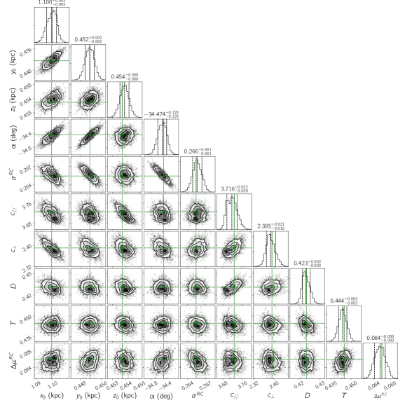
In Section 5, we tested our fitting procedure on a mock catalogue and proved that it successfully recovered the input values. We thus expect, within the limitations of the model and of the luminosity function assumptions, to have found the true values of the Bulge density distribution. Nonetheless, we execute an additional check of the results and of their statistical errors with a Markov chain Monte Carlo (MCMC) in a Bayesian framework. In Figure 21 in the Appendix we compare the results (green dots) obtained using the L-BFGS minimisation method and an MCMC, for model $S$ (label ‘$\sigma^{\mathrm{RC}}$ free’ in Table 3, see discussion in Section 7.1).

We have used the Affine Invariant MCMC Ensemble sampler emcee (Foreman-Mackey et al., 2013) to explore the full posterior distribution with 30 walkers. The contours of the two-dimensional projection of the posterior probability distribution of the parameters of model $S$ are nearly Gaussian (Figure 21), but there is a clear correlation between the scale-lengths of the Bulge density law, and $\sigma^{\mathrm{RC}}$ and the viewing angle $\alpha$. The marginalised distribution for each parameter is shown along the diagonal and the 0.5 quantiles with the upper and lower errors (16% and 84% quantiles) are given above each 1-D histogram. For the initial state of the Markov chain we chose the best-fit results reported in Table 3 for model $S$, label ‘$\sigma^{\mathrm{RC}}$ free’: with 30,000 iterations (20% of the chain was discarded as burn-in) and an acceptance fraction of 43%, the final results and errors on the parameters are in complete agreement with the values found with the L-BFGS method. The statistical errors are equally small and, as can be seen from Figure 20 showing a sample of 10 chains for 8 parameters, they converge to a value close to the initial one (the blue line in Figures 21 and 20). We note that Wegg et al. (2015) also report small statistical errors: “We have performed an MCMC to estimate errors on both the model parameters (…) The resultant statistical errors are extremely small, significantly smaller than the difference between fits with different models. We therefore consider the statistical errors to be negligible in comparison to systematic errors".

There may exist various causes for the systematic errors: the extinction related dispersion and photometric errors (see Figure 4); confusion of point sources in overcrowded regions; clssification and calibration errors; and the fact that the model is not an exact description of the data. In addition, at the end of Section 5, we have shown that the choice of the Bulge density distribution alone can introduce systematic errors larger than the standard errors.

The next subsections look into more detail at the models reported in Table 3 and their suitability in describing the data.

6.5 Data versus model comparison

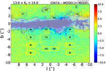
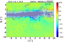
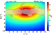
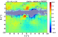
We here discuss Figures 10-15, which show the data and the best-fit models (labeled ‘main’ in Table 3) in different projections.

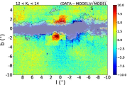
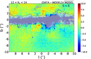
The log likelihood values in Table 3 suggest model $E$ performs slightly better than model $S$; however, there are many similarities between the two sets of results: for both, we obtain $\alpha\simeq-19.5^{\circ}$ and axis ratios [1:0.44:0.31]. As we will see in the residual maps, a two component model ($S+E$) provides a better description of the data especially in the inner regions, but at the expense of a larger number of free parameters.

Using the first data release of the VVV, Wegg & Gerhard (2013) fitted exponentials to the density profiles of the major, intermediate and minor axes shown (see their figure 15) and found scale lengths of 0.70, 0.44 and 0.18 kpc respectively, corresponding to axis ratios [1:0.63:0.25]. In the Discussions section we compare our results with other literature estimates for the shape and viewing angle.

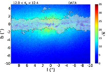
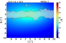
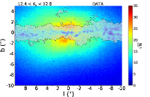
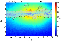
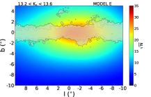
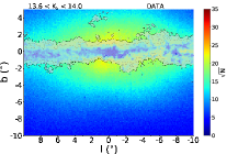
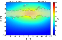
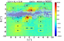
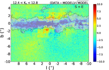
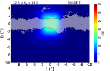
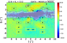
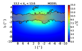
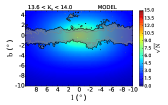
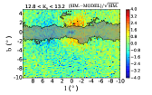
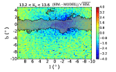
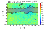
In Figure 10 we show the number density distribution of VVV stars in five magnitude bins (left column) and the best-fit models $E$ and $(S+E)$ in Galactic coordinates (middle and right column respectively). Model $S$ is very similar to model $E$ and thus not shown. A magnitude slice is almost equivalent to selecting stars within a certain distance range, where the brightest magnitude slice $12<K_{s}<12.4$ selects the nearest stars, in front of the Bulge, and the faintest magnitude slice $13.6<K_{s}<14.0$, selects the furthest stars, behind the Bulge.

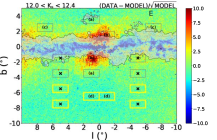
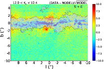
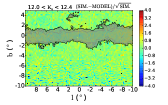
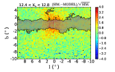
The middle and right panels of figure 11 show the difference between the data and the $E$ and $S+E$ models, divided by the Poisson noise in the model, ($N_{i}$-$M_{i}$)/$\sqrt{M_{i}}$, for each magnitude bin. The addition of the second component $E$ (left column) improves the fit in the central region, especially in the bright magnitude slice (top right panels of Figure 11). Model $S+E$ assumes a young population (5 Gyr), described by model $E$ and an old one (10 Gyr), described by model $S$, which is the main component. The younger component has a $0.1$ mag brighter peak than the 10 Gyrs old population (see Figure 3 where $\mu_{5}^{\mathrm{RC}}=$ -1.64, hence $\mu_{5}^{\mathrm{RC}}=$ -1.74 after applying the $\Delta\mu^{\mathrm{RC}}=-0.1$ shift), which helps to provide a better fit in the central regions of the brighter magnitude bins. The LFs for both populations are shown in the right panel of Figure 3, where the integrated area under each curve gives the total number of stars expected for each component for the best fit parameters. We provide several interpretations for the additional component in Section 7.

To summarise our results, we show the residuals for all three models in one magnitude slice in Figure 12. As previously observed, models $E$ and $S$ do not provide a good match for the data in the area close to the Galactic Centre, $|b|<3^{\circ}$ and $|l|<2^{\circ}$, though in general they perform very well. The model $(S+E)$ matches the observed distribution remarkably well (with a median percentage residual of 5 %) apart from some discrepancies within the central tiles $b306$, $b320$, $b347$. It is not clear at this stage whether this is entirely due to data processing or calibration issues or possibly some real feature present in the central data.

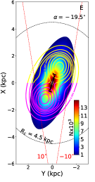
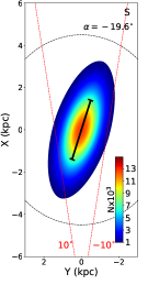
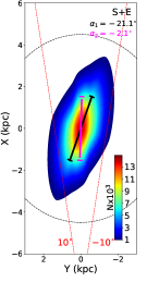
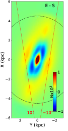
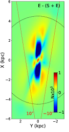
The best-fit density laws projected along the Z-axis (bottom panels) and X-axis (top panels) for the models $E$, $S$ and $S+E$ (first three columns of the figure) are shown in Figure 13. On the figure, we mark the cut-off radius $R_{c}$, the viewing angle, and the limiting longitudes of the VVV survey. Overlaid on model $E$, we add a density law that is a complex parametrisation of the Bulge X-shaped component, provided by López-Corredoira (2017) in their equation 4. This model predicts a double RC at intermediate latitudes. We only show a slice of the density law within $-0.7<Z/$kpc$<-2.0$ (below the red line in the Y-Z plane) corresponding to $b<-5^{\circ}$, projected onto the X-Y plane. The density contours of the foreground RC (X < 0) are marked in violet and those of the background RC (X > 0) in yellow. The same colour scheme is adopted for the Y-Z plot projection where we do not make any Z cuts, to show that the nearer RC will be dominant at positive longitudes while the further RC will be dominant at negative longitudes, symetrically above and below the plane. In addition, we can expect: 1) the contribution to the magnitude distribution of the background RC to diminish as the longitude to increase towards positive values, as the contribution of the foreground RC increases and 2) the separation between the two RCs in the magnitude distribution to increase as we look away from $l=0^{\circ}$. This separation will depend on the angles formed by the X-shape with the GP as well as on the Galactic coordinates or distance from the Galactic plane.

The Y-Z distributions display a ’boxy’ Bulge with a flattened distribution along the Z direction. The difference between the $E$ and $S$ models (fourth column) illustrates that the $E$ density law is more centrally concentrated. The $E$ - $(S+E)$ residuals in the X-Y plane (fifth column) are irregular because the two components in the $S+E$ model have different viewing angles.

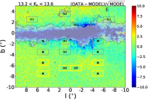
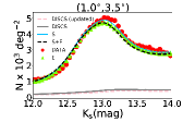
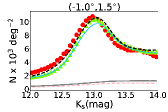
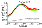
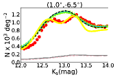
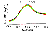
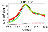
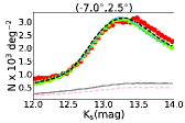
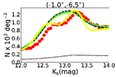
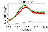
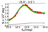
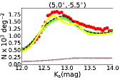
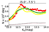
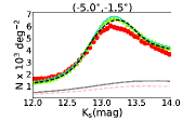
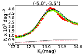
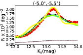
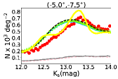
In Figure 14 we show 8 examples of magnitude distributions in $2^{\circ}\times 1^{\circ}$ fields where the data points we fit are the red circles and the best-fit models are represented with a black dotted line (model $S+E$), green triangles (model $E$) and a thin blue line (model $S$). The disc populations are shown in gray (the updated discs, discussed in Section 7.2, in pink). The centres of the fields are marked with letters in the middle column of Figure 11, where each letter represents a column of Figure 14. The panels are organised as follows:

• column (a) shows the magnitude distributions in two symmetric fields centred at $(l,b)=(1^{\circ},3.5^{\circ})$ and $(l,b)=(1^{\circ},-3.5^{\circ})$: the star counts are symmetric with respect to the Galactic Plane and there is good agreement between the data and the best fit model.

• column (b) shows the magnitude distributions in two tiles ($b306$ and $b347$) that have pronounced residuals in Figure 12 with centres at $(l,b)=(-1^{\circ},1.5^{\circ})$ and $(l,b)=(1^{\circ},-1.5^{\circ})$, though interestingly these are symmetric with respect to the Galactic Centre. The fit is poorest in the first two brighter magnitudes slices, which produce the overdensities observed in the top panels of Figure 11. As we have shown, adding an extra component partially solves the problem: model $S+E$ gives the best fit to the data in central regions, making the overall fit for the bright magnitude slices better, as can be seen in the top right panels of Figure 12.

• column (c) shows the magnitude distributions in symmetric fields with respect to $l=0^{\circ}$, centred at $(l,b)=(7^{\circ},2.5^{\circ})$ and $(l,b)=(-7^{\circ},2.5^{\circ})$. The peak of the RC is shifted between positive (bright RC) and negative (faint RC) longitudes, a consequence of the orientation of the Bulge with regard to the Sun-GC direction.

• column (d) shows magnitude distributions in two fields at intermediate latitudes, centred at $(l,b)=(1^{\circ},-6.5^{\circ})$ and $(l,b)=(-1^{\circ},-6.5^{\circ})$. In these fields, the double RC is clearly visible in the VVV data as already shown by previous studies (e.g. Saito et al., 2012). Because the fields are symmetrical to $l=0^{\circ}$, the two RCs contribute similarly to the magnitude distribution, even though the foreground RC will contributes slightly more to the distribution at $l=1^{\circ}$ compared to $l=-1^{\circ}$; for the background RC, the opposite is true. The X-bulge density law proposed by López-Corredoira (2017) describes well this phenomenon: by looking at Figure 13, we can clearly see how the $l=1^{\circ}$ line of sight will pass closer to foreground RC than to the background RC, but thanks to the viewing angle under which we observe the Bar, both RCs will be visible in the magnitude distribution, even though in different contributions. The double peaked magnitude distribution shown in yellow is the López-Corredoira (2017) model calculated using Equation 4 where $\rho_{\mathrm{B}}$ is the X-shaped density distribution that we have shown in Figure 13. The model is successful at predicting the double RC, as expected.

We now explore the signal of the double RC at intermediate longitudes $l=\pm 5^{\circ}$ and varying distance below the GP by comparing the data with our models and the model based on the X-shaped density law (which should be accurate for $b<-5^{\circ}$) in Figure 15. The centres of the $2^{\circ}\times 1^{\circ}$ fields are marked with ‘x’ in Figure 11. The top and bottom rows show the apparent magnitude variations at constant longitudes, $l=5^{\circ}$ and $l=-5^{\circ}$ respectively, with the latitude decreasing from left to right between $-1.5^{\circ}$ and $-7.5^{\circ}$.

The fields close to the Galactic Plane (first column, $-2^{\circ}<b<-1^{\circ}$) are largely incomplete because we mask the high extinction regions, thus the amplitude of the RC is not well fitted (please note that this is the result of the global fit). At $-4^{\circ}<b<-3^{\circ}$ (second column) the models perform well but at lower latitudes $-5^{\circ}<b<-6^{\circ}$ (third column), where the double RC becomes visible, we can clearly see the amplitude of the RC peak in the data is not well matched by the model. The excess of stars supposedely belongs to the peanut shape that is not well represented by a single simple triaxial shape. Even further from the Galactic Plane, where the number counts are much lower (fourth column, $-7^{\circ}<b<-7^{\circ}$), the discrepancy is more obvious at all magnitudes.

At $b<-5^{\circ}$, the model using the X-shaped density law (López-Corredoira, 2017) is doing a better job at predicting the magnitude distribution. However, while the model predicts a double RC, the data only shows one. This could be explained if the second RC contributed less than predicted by the López-Corredoira (2017) model at intermediate longitudes (this could easily be the case, e.g. imagine a $l=5^{\circ}$ line crossing the X-Y plane in Figure 13). From the magnitude variation of the peaks at constant longitude (left to right), it is clear that with increasing distance from the plane the foreground RC gets brighter (positive longitude, top row) and the background RC gets fainter (negative longitude, bottom row), behaviour specific to an X-shaped distribution.

Table 4: Best fit parameters variation for model $S$ as a function of $\sigma^{\mathrm{RC}}$. We fitted model $S$ using LFs with increasing $\sigma^{\mathrm{RC}}$ in steps of 0.03 mag; in the last row, $\sigma^{\mathrm{RC}}$ is a free parameter. These values are shown in Figure 16.

ln($L_{P}$)	$\sigma^{\mathrm{RC}}$	$\alpha$	$x_{0}$ , $y_{0}$, $z_{0}$, $c_{//}$, $c_{\perp}$
36,731,464	0.06	-19.36	1.48, 0.63, 0.47, 3.00, 1.88
36,731,560	0.09	-20.09	1.46, 0.62, 0.47, 3.06, 1.87
36,735,035	0.12	-21.14	1.42, 0.61, 0.47, 3.13, 1.88
36,737,262	0.15	-22.64	1.37, 0.59, 0.47, 3.31, 1.90
36,739,532	0.18	-24.69	1.30, 0.57, 0.46, 3.37, 1.95
36,741,544	0.21	-27.40	1.23, 0.54, 0.46, 3.52, 2.03
36,743,487	0.26	-34.40	1.10, 0.45, 0.45, 3.58, 2.09

To roughly quantify what proportion of the VVV stars are found in the X-shaped residuals relative to the total number of Bulge stars, we consider the fields at intermediate latitudes, outside $|b|<4^{\circ}$. Here the feature is most clearly visible in the VVV data, even though it may continue to lower latitudes. The model tends to overfit the region between the X-shape arms (see blue depression at $l=0^{\circ}$ in Figure 12) and underfit the X-shape arms themselves, hence we conjecture that the model has to be reduced by some fraction $<1$ such that only $\sim$5% of the residuals are negative, the positive excess that remains, would theoretically belong to the arms. With this assumption and mirroring the region at $b<-5^{\circ}$ to positive latitudes, $b>5^{\circ}$, we find that $\sim 7$ % of the stars belong to the X-shaped arms relative to the entire modelled Bulge, within $-10^{\circ}<l<10^{\circ},-10^{\circ}<b<10^{\circ}$.

Figure 16: Best fit parameters variation as a function of increasing $\sigma^{\mathrm{RC}}$ with a step of 0.03 mag (each identified with a different colour), for model $S$. The result for $\sigma_{\mathrm{free}}^{\mathrm{RC}}=0.26$ mag (free parameter) is marked in green. $Left$ $panel$: as $\sigma^{\mathrm{RC}}$ increases, the fitted viewing angle $\alpha$ also increases. $\alpha$ is the most affected parameter by the $\sigma^{\mathrm{RC}}$ variation. $Middle$ and $right$ $panels$: the parameters controlling the shape of the density distribution are not affected by the choice of $\sigma^{\mathrm{RC}}$ even though a tiny trend can be observed. We also add the results of Wegg & Gerhard (2013) (WG) and Cao et al. (2013).

7 Discussion

7.1 The Luminosity function

7.1.1 Variations of the LF

The intrinsic LF of the Bulge is sensitive to both age and metallicity variations but in absence of accurate and consistent measurements of these quantities across the Bulge, we do not attempt to build a spatially varying LF.

The main effect of not having a simple Bulge population as the one we assumed in Section 4.3, will be to blur the intrinsic LF. We therefore convolve the Galaxia generated LF with a Gaussian kernel of $\sigma$ as a free parameter (therefore $\sigma_{\mathrm{free}}^{\mathrm{RC}}$ $=\sqrt{\sigma^{2}+(\sigma^{\mathrm{RC}})^{2}}$ becomes a free parameter, where $\sigma^{\mathrm{RC}}=0.06$ mag) and re-fit the VVV data with models $E$ and $S$. The best fit results are listed in Table 3 for both models and are labeled ‘$\sigma^{\mathrm{RC}}$ free’.

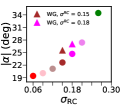
Compared to the approach presented in this paper, Wegg & Gerhard (2013) followed a different route and attempted to constrain the Bulge properties non-parametrically. Instead of estimating the parameters of a Bulge density law, they deconvolve the observed RC magnitude distributions to extract line-of-sight RC densities from which they build a 3D map assuming eight-fold mirror symmetry. The result they obtained, $\alpha=(-26.5\pm 2)^{\circ}$, falls in the middle of our extreme values for $\sigma^{\mathrm{RC}}=0.06$ mag, $\alpha=-19.4^{\circ}$ (red dot) and $\sigma_{\mathrm{free}}^{\mathrm{RC}}=0.26$ mag, $\alpha=-34.4^{\circ}$ (green dot).

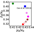
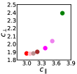
In absence of a fully reliable calibration of the Bulge RC dispersion in literature (the latest measurement in the local neighbourhood with Gaia finds $\sigma^{\mathrm{RC}}=0.17$ mag - see Hawkins et al. 2017), we investigated the effect of the $\sigma^{\mathrm{RC}}$ variation on the density law parameters by convolving the Galaxia generated LF with a Gaussian of increasing $\sigma$ in order to obtain $\sigma^{\mathrm{RC}}=0.09,0.12,0.15$, 0.18 and 0.21 mag for a 10 Gyrs population. The results shown in Figure 16 and listed in Table 4 confirm the expectation that a higher $\sigma^{\mathrm{RC}}$ is responsible for a higher viewing angle $\alpha$. This was also observed by Wegg & Gerhard (2013) who found $|\alpha|$ reduces from 26.5^∘ to 25.5^∘ (triangles in Figure 16) when $\sigma^{\mathrm{RC}}$ decreseas from 0.18 to 0.15 mag and explain ‘this is because increasing the line-of-sight geometric dispersion has given the illusion that the bar is closer to end on’. We find a stronger dependence of the viewing angle on $\sigma^{\mathrm{RC}}$, with $\alpha$ decreasing from 24.69^∘ to 22.64^∘ for the same $\sigma^{\mathrm{RC}}$ variation. Our work is probably more sensitive to the viewing angle as we do not need to assume eight-fold mirror symmetry thanks to continuous coverage in all quadrants of the newer VVV data release.

While the viewing angle is strongly dependent on $\sigma^{\mathrm{RC}}$, the axis ratios do not vary significantly as seen in the middle and right panels of Figure 16. In fact, the parameters controlling the shape of the density distribution are not significantly affected by the choice of $\sigma^{\mathrm{RC}}$ even though a trend can be observed in the middle and right panels of the figure: in the middle panel, as the $\sigma^{\mathrm{RC}}$ increases (the values are colour-coded as in the left panel) the bar gets puffier in both the vertical and $Y$-axis directions but as it reaches $\sigma^{\mathrm{RC}}=0.15$ mag it starts to get thinner again along the $Y$-axis while it continues to get thicker in the vertical directions. The parameters controlling the shape of the distribution are also correlated, with $n$ decreasing as $\sigma^{\mathrm{RC}}$ increases while the $c_{\parallel}/c_{\perp}$ ratio also increases. Notice that these variations are tiny and do not change the shape of the distribution significantly, the viewing angle $\alpha$ being the most affected parameter.

Figure 17: Comparison of the axis ratios ($y_{0}/x_{0}$ and $z_{0}/x_{0}$ in the $left$ and $right$ $panels$) and Bulge viewing angle $\alpha$ obtained in this work for a one component fit (model $E$, red star), with previous studies. The error bars (in red) mark the maximum variation produced in our results by varying $\sigma^{\mathrm{RC}}$ (see also Figure 16). Literature results prior to 2009 (Vanhollebeke et al., 2009), are marked with black dots and the error bars are shown when reported. More recent measurements are shown with different colours: the results from a non parametric Bulge study using VVV RC stars with magenta (Wegg & Gerhard, 2013), those from a parametric study using 2MASS giants with cyan (Robin et al., 2012) and the results from two OGLE separate studies, with RR Lyrae (Pietrukowicz et al., 2015) and RC stars (Cao et al., 2013), with yellow and blue respectively.

7.2 The discs

7.2.1 The thin disc

In Galaxia, the thin disc density distribution has a scale length of $R_{d}=2.53$ kpc and a disc hole scale length of $R_{h}=1.32$ kpc. More recently, Robin et al. (2012) used 2MASS photometry to fit simultaneously for the parameters of the Bulge population and the shape of the inner disc. The updated parameters of the thin disc in the best Bulge model (model $S+E$, see their table 2) are $R_{d}=2.17$ kpc and $R_{h}=$ 1.33 kpc: the disc hole scale length is almost identical and the disc scale length is shorter by 400 pc compared to the previous values.

7.2.2 The thick disc

Robin et al. (2014) used photometric data at high and intermediate latitudes from SDSS and 2MASS surveys to re-analyse the shape of the thick disc. Their updates include a new IMF best fit, $dN/dm\propto m^{-0.22}$, a slightly smaller scale height of $h_{Z}=($535.2 $\pm 4.6$) pc and a shorter scale length of $h_{R}=($ 2362 $\pm 25$) pc plus a new age best fit of 12 Gyrs.

We have performed all the fits described in the manuscript with the updated thin and thick discs versions and the results are reported in last rows of Table  3. They are also shown in pink in Figures  14 and  15. Finally, we have decided to use the default (Robin et al., 2003) values throughout the paper, for the following reasons:

• In the fitting procedure we exclude the area close to the Galactic plane where the reddening $E(J^{\prime}-K^{\prime}_{s})$ is higher than 1 mag and where the majority of the thin disc population lies. The $E(J^{\prime}-K^{\prime}_{s})=1.0$ contour extends, on average, to latitudes $-1.5^{\circ}<b<1.5^{\circ}$ (see Figures 1 and 2) which is equivalent to a height perpendicular to the Galactic plane of $-0.2<Z$/kpc$<0.2$ at 8 kpc. This region is masked out in the fitting procedure described in Section 6. The scale height of the oldest thin disc component is $\sim$ 300 pc, therefore a large part of the thin disc population is excluded from the fit.

• The fitting results confirmed that the Bulge density law parameters remain almost identical, regardless of the discs (original or updated version) assumed;

• To avoid multiple modifications to the $Galaxia$ code.

7.3 Stellar Mass of the Bulge

Galaxia relies on the isochrones table as input to the code to assign a mass to each star produced as part of the mock catalogue for a given IMF. Pietrinferni et al. (2004) undertook a detailed analysis of the outer Bulge stellar density and LF, assuming a Salpeter (1955) IMF, by fitting model parameters to a set of 94 windows in the outer Bulge situated at $-8^{\circ}<l<10^{\circ}$ and $b<|4|^{\circ}$ in the DENIS survey. The same IMF was used in the Besancon model and implemented in $Galaxia$. The Bulge stars lie at distances between 4 and 12 kpc, corresponding to absolute magnitudes $M_{K}$ in the range -3.5 to 1 mag in the 12 to 14 apparent magnitude range $K_{s}$. At these bright magnitudes, the intrinsic luminosity function is not influenced by the choice of IMF therefore using a different IMF would not change the results in Table 3.

The stellar mass in the Bulge is however sensitive to the IMF choice. We calculate the mass of the Bulge assuming a bottom light Chabrier IMF, similar to a Kroupa IMF, which we have used throughout the paper. The slope of the latter becomes significantly shallower than the Salpeter IMF below 1 M_⊙ and describes more accurately observations in the Galactic Bulge (see also Section 4.3). The majority of stars in the Bulge have masses $<1M_{\odot}$ so we would expect to greatly overestimate the total mass of the Bulge using a Salpeter IMF. In addition, Sharma et al. (2016) test the theoretical predictions of $Galaxia$ with asteroseismic information for 13,000 red giant stars observed by Kepler and find that the distribution of the masses predicted by the $Galaxia$ Galactic model overestimates the number of low mass stars. We therefore report the Bulge mass estimates using the Chabrier IMF which is similar to the Kroupa IMF, excluding the Salpeter IMF.

Using the best-fit model ($E$) in $Galaxia$ we can predict the fraction of Bulge stellar mass in the RGB and the RGB luminosity that we should observe within the VVV coverage, with the colour-magnitude cuts $0.4<J-K_{s}<1.0$ - $12<K_{s}<14$, and hence use the observed population (and the measured fraction) to constrain the total stellar mass of the Bulge. For a given IMF the PARSEC isochrones enable us calculate the remnant population and therefore the total mass of the original population. For the total MW Bulge mass, we obtain $M_{\mathrm{Bulge}}^{\mathrm{Chabrier}}=2.36\times 10^{10}M_{\odot}$, including the mass of the remnants (49% of the total mass of the Bulge) using a Chabrier IMF. For the two component $S+E$ best fit, we obtain 2.21 $\times 10^{10}$ M_⊙ ($S$ component) and 1.2 $\times 10^{9}$ M_⊙ ($E$ component), for Chabrier IMFs. If the low-latitude residuals are caused by the presence of an extra component (component $E$), then this component would contribute $\sim$5% to the total Bulge mass budget.

Other recent measurements of the Bulge stellar mass include:

• Robin et al. (2012) who estimate the total mass of the Bulge by fitting a population synthesis model to 2MASS and for the two component best fit, find $M_{\mathrm{Bulge}}=6.36\times 10^{9}$ M_⊙ where the mass of the $S$ component is 6.1 $10^{9}M_{\odot}$ and the mass of the smaller component $E$ is 2.6 $\times 10^{8}$ M_⊙.

• Portail et al. (2015) construct dynamical models of the MW Bulge using RC giants and kinematic data from the BRAVA survey. They compute the total mass of the Galactic Box/Peanut Bulge and find a stellar mass $M_{Bulge}=1.25-1.6\times 10^{10}M_{\odot}$, depending on the total amount of dark matter in the Bulge. Wegg et al. (2015) use a Kroupa IMF at 10 Gyrs and report a Bulge mass estimate of 1.81 $\times 10^{10}M_{\odot}$ that includes, in addition to a Bulge population, a thin and a superthin bar.

• Valenti et al. (2016) scale the total magnitude distribution obtained from all VVV fields (320 square degrees) to the one from Zoccali et al. 2003 (an 8${}^{\prime}\times$8^′ field at $(l,b)=(0^{\circ},-6^{\circ})$), to obtain a stellar mass of $M_{Bulge}=2\times 10^{10}M_{\odot}$. They find that a $\pm 0.3$ dex variation in their assumed IMF slope $\alpha=-1.33\pm 0.07$ (Zoccali et al., 2000), would change the mass estimate by less than 12%; moreover the authors assume constant disc contamination. In contrast we included in our model the disc contamination which is calculated as a function of field and magnitude.

7.4 Structural comparison with previous results

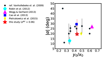
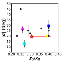
Figure 17 compares the Bulge parameters measured in this work to those obtained in other studies with a variety of tracers, e.g. RR Lyrae, Mira variables and RC stars. Note that the results of modelling the Galactic Bulge with an exponential and sech² density laws as reported in Table 3 are indistinguishable and are marked in red in Figure 17. The red error bars give the maximum variation seen in the parameters as a result of varying $\sigma^{\mathrm{RC}}$: only the viewing angle seems to be significantly affected (see Figure 16).

We take advantage of a large catalogue of Bulge studies up to 2009 in Vanhollebeke et al. (2009) to show the range of the viewing angle values and the axis ratios with black dots, adding the error bars when present. Additionally, four more recent results are marked with colours: one from a parametric model describing the 2MASS data (cyan, Robin et al., 2012), one from a non-parametric study of VVV RC stars (magenta, Wegg & Gerhard, 2013), and two from the OGLE survey, with RRLyrae (yellow, Pietrukowicz et al., 2015) and RC stars (blue, Cao et al., 2013). Robin et al. (2012) obtain an orientation of about 13^∘ for the main structure, in their two-component fit. Cao et al. (2013), who use number counts of red clump giants from the OGLE III survey to fit triaxial parametric models for the Bulge, obtain axis ratios within the parameter space spanned by our results when testing different $\sigma^{\mathrm{RC}}$; we mark their result in both Figures 16 and 17.

7.5 Central region

As in previous studies (e.g. Robin et al. 2012), we find that one-component Bulge models do not provide a good match to the data in the central Galactic regions. We notice a clear overdensity at $|b|<3^{\circ}$ and $|l|<2^{\circ}$ (left and middle panels in Figure 12). The match between the model and the data can be improved by considering a combination of two populations (right panel in the same figure), where the central one has a RC peak brighter than the RC peak of the main population.

The presence of the overdensity can be explained using several theories:

• the presence of a ‘disky’ pseudo-Bulge - in addition to a ‘boxy’ Bulge (Dwek et al., 1995), our Galaxy might host a ‘disky’ pseudo-Bulge, observed in many early and late type b/p Bulge galaxies (Bureau et al 2006). These types of Bulges grow ‘secularly’ out of disc gas that was transported inwards along the bars (e.g. Kormendy & Kennicutt, 2004). The centrally concentrated residuals with short vertical scale height we observe might be indicative of this type of disc-like, high density pseudo-Bulge, also seen in N-body models by Gerhard & Martinez-Valpuesta (2012). In addition, a change-of-slope at $|l|\sim 4^{\circ}$ can be seen in the VVV RC star count maxima longitude profiles close to the Galactic plane (see Gerhard & Martinez-Valpuesta 2012) while further from the Galactic Plane, the change in slope disappears. Gerhard & Martinez-Valpuesta (2012) argue that a pseudo-Bulge does not need the presence of a secondary nuclear bar to explain the change of slope in the longitude profile.

• spiral arms / thin bar overdensity - the bar and buckling instabilities in the stellar disc lead to a boxy Bulge which extends to a longer in-plane bar (Athanassoula, 2005). The bar couples with the spiral arms in the disk, giving rise alternatively to leading, straight, or trailing bar ends (Martinez-Valpuesta et al., 2006). It is possible that a density enhancement produced by spiral arms along the Sun-GC line-of-sight might explain the residuals observed in Fig 11 (the spiral arms are confined to the Galactic plane but a height of 100 pc would subtend an angle of $\sim 1.5^{\circ}$ at 4 kpc, while the same vertical height would only subtend $\sim 0.7^{\circ}$ at 8 kpc).

• the discs - we have used a 2D reddening map to correct for the effects of extinction, assuming all the sources are behind the dust. Disc objects (e.g. nearby dwarfs) or Bulge stars that are not behind all the dust (and are situated between the Sun and the Galactic Centre) will be over-corrected by various amounts, which could possibly lead to an apparent overdensity in the central regions of the Bulge in the bright magnitude slices that contain the sources closest to the Sun. We have tested this hypothesis by adding 3D extinction to a sample of Galaxia generated mock thin disc stars. We have then corrected for extinction using a 2D map, therefore considering only the highest value of the 3D map. If this method was accurate, the number density of the 2D extinction corrected sample should coincide with that of the initial mock sample. Instead, we found only a 4% increase in the number of counts in the $12.0<K_{s}<12.8$ magnitude range after correction for the stars near the plane but for stars with $|b|>1.5^{\circ}$ no increase was found. We thus believe that using a 2D reddening map does not produce the central overdensity observed.

• younger central population - altering the disc parameters does not improve the agreement between data and model in the magnitude range considered ($12<K_{s}<14$). We can only account for it by adding an extra component with a smaller size ([ $x_{0},y_{0},z_{0}$] = [1.52, 0.24, 0.27] kpc) and a brighter RC, with $\Delta M=0.1$ between the main component and the secondary one. A younger population, of 5 Gyrs and solar metallicity (as the main population), would produce such a shift but it could also be achieved considering other combinations of ages and metallicities between the two populations. The presence of a young population inside the Bulge is not inconsistent with simulations (e.g. Ness et al., 2014) and Miras variable (e.g. Catchpole et al., 2016) observations.

Figure 18: N-body simulation from Shen et al. (2010) ($top$ $row$), model prediction ($middle$ $row$) and residuals between the simulation and the model ($bottom$ $row$). The size of the bin is 12’ x 12’, double the bin size used for the data, and the viewing angle of the model is 15 ^∘. The residuals in the brightest slice $12.0<$K${}_{s}<12.4$ ($first$ $column$) do not show the central excess seen in the data (top row of Figure 11). The residuals in the second slice ($second$ $column$) $12.4<$K${}_{s}<12.8$, show an overdensity in the simulation running diagonally from the centre towards the left, both at positive and negative latitudes; the same feature can be observed in the data residuals (second row of Figure 11), but mainly at negative latitudes and positive longitudes. At fainter magnitudes, the residuals show the model overpredicts the number of counts on each side of the GC; however, in the last two slices, the overprediction is dominant at negative latitudes, near the GC, similarly to what is observed in the data (fourth row of Figure 11).

7.6 The X-shape of the Bulge: testing the model on a Peanut Bulge N-body simulation

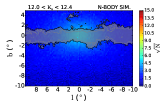
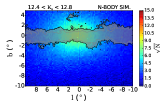
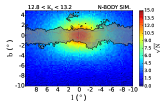
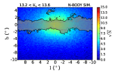
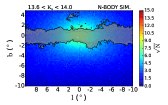
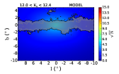
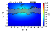
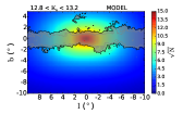
In this work we have not implemented a parametric description of the X-shaped component which is apparent in the RC population (e.g. Ness & Lang, 2016). To test if our model is capable of robustly recovering basic parameters such as the orientation angle in realistic mock Bulges, we test its performance on an N-body model (Shen et al., 2010) that has been shown to predict the split Red Clump (Li & Shen, 2012). Li & Shen (2012) found that 7% of the light in the whole boxy Bulge region resided in the X-shaped structure. To use the same observables (the number density distribution in different $K_{s}$ magnitude ranges) as in the VVV, we convolve the N-body model with the Bulge LF, $\phi_{B}$.

The N-body model has $\sim$1 million particles but within the VVV footprint only $\sim$400,000 remain. Because of the low number of particles, we have performed two fits, one using 6^′ $\times$ 6^′ bins as in the data, and one with double the bin size 12^′ $\times$ 12^′. The simulation, the best-fit model and the residuals are shown in Figure 18, for the larger bin size needed to satisfy our assumption that the measurements are distributed according to a Gaussian function. We also mask the high reddening regions to mimic the data-fitting procedure, but exclude the discs as they do not contribute significantly to the simulation. The model therefore, contains only the analytic form of the Bulge. Using the larger bins 12^′ $\times$ 12^′ we find a viewing angle of 15 ^∘, on the lower end of the expected value of $20_{-5}^{+5}$ degrees for the simulation while with the smaller bins we find $\alpha=20^{\circ}$. Nataf et al. (2015) also test their model on this N-body simulation, assuming four viewing angles $\alpha=0^{\circ},15^{\circ},30^{\circ},45^{\circ}$ and find that $\alpha=30^{\circ},45^{\circ}$ provide the best fit, with $\alpha=15^{\circ}$ being nearly as consistent.

The fit in the central regions of the brightest slice $12.0<$K${}_{s}<12.4$ is good, suggesting that the overdensity observed in the data does not belong to a structure specific to the peanut Bulge which we could not fit due to our simple assumption of a triaxial Bulge. In the second slice, $12.4<$K${}_{s}<12.8$, there is an overdensity in the simulation running diagonally from the centre towards the left, both at positive and negative latitudes; the same feature can be observed in the data residuals (see Figure 11), but mainly at negative latitudes and positive longitudes (see alse the residuals for the WISE survey, in figure 3, Ness & Lang 2016). Due to the orientation of the Bulge, the arms of the X-shape appear asymmetric, with the arms at positive latitudes more visible in the residuals while the arms further from the Sun, behind the Galactic centre, almost invisible. This is only a projection effect caused by the orientation of the Bulge as discussed in the previous Section. At fainter magnitudes the model overpredicts the number of counts at intermediate longitudes on each side of the Galactic centre; however in the faintest two slices the underdensity is observed mainly at negative latitudes, $-2^{\circ}<l<-6^{\circ}$ and $-3^{\circ}<b<3^{\circ}$, in the same region as in the data but slightly closer to the Galactic centre. The overdensity in the model is created by the redistribution of the total number of stars present in the peanut Bulge into a boxy shape which the model is constrained to have.

Other tracers such as F dwarfs ($<$ 5 Gyrs old, López-Corredoira 2016), RR Lyrae ($>$ 10 Gyrs old, e.g. Kunder et al., 2016; Gran et al., 2016) and short period Mira variables (old stars, see Catchpole et al., 2016; López-Corredoira, 2017) do not trace the X-shaped component, thus emphasizing that the mechanism and the time of formation of the Galactic Bulge are not 100% clear.

8 Conclusions

We have used a parametric approach to find the best analytic function that describes the 3D Bulge density observed by the VVV survey in the NIR. We test our modeling methodology on a range of mock datasets, including those generated using self-consistent simulations of the Milky Way Galaxy. We thus prove that the technique delivers robust results and take care to quantify random and systematic uncertainties associated with the method. Our best-fit model produces a faithful representation of the stellar density field in the inner Galaxy, with reassuringly low levels of residuals across the entire VVV field of view.

With find the Bulge/Bar to be “boxy”, with an axis ratio of [1:0.44:0.31] and an angle between the major axis and the Sun-Galactic Centre line of sight of $\sim$20 degrees (top row, Table 3). We show that there exists a strong degeneracy between the viewing angle and the dispersion of the RC absolute magnitude distribution. To reproduce the stellar line-of-sight distribution at a range of locations on the sky, models with larger intrinsic RC dispersions prefer larger viewing angles. We demonstrate that as a result of the degeneracy, assuming $\sigma^{\mathrm{RC}}=0.18$ leads to inferring viewing angles of $\sim 25^{\circ}$ (closer to the value reported in Wegg & Gerhard, 2013, $\alpha=($-26.5$\pm 2)^{\circ}$). However, in the analysis presented here, we also found evidence for a much larger intrinsic dispersion of the RC absolute magnitudes in the Bulge area, namely $\sigma_{\mathrm{free}}^{\mathrm{RC}}\sim 0.26$, larger than the latest measurment in the solar neighbourhood ($\sigma^{\mathrm{RC}}=0.17$ mag, Hawkins et al. 2017) where the younger thin disc population is dominant. We envisage that with new next-generation Bulge surveys it should be possible to measure the true $\sigma^{\mathrm{RC}}$ across the Bulge and thus, at last, settle the viewing angle argument.

The most pronounced residuals of the one-component Bulge model appear to cluster tightly in the central regions of the Galaxy. One interpretation of this residual density distribution is that the core portions of the Bulge are better described by a combination of two triaxial components: the main old one and a younger smaller one (last two rows, Table 3). Apart from this additional small-scale ellipsoidal component indicated by the low-latitude counts of the VVV RC giants, the only other noticeable outlier is the pattern induced by the split RC. We choose not to augment our Bulge model with an ingredient responsible for the cross-shaped pattern, but provide an estimate of the total stellar mass locked in this population. We show that $\sim 7\%$ of the total Bulge/Bar could be residing in this non-ellipsoidal constituent, in agreement with some of the numerical simulations of the Galactic Bar ( e.g. Shen et al., 2010). However, this is probably only a lower estimate of the total fraction of stars contributing to the X-shape as it does not include the stars on orbits that could be fit within the triaxial component.

Finally, the mass of the Bulge/Bar is a key ingredient in the recipe for the total density distribution of the Milky Way. The Bulge mass has to satisfy microlensing constraints (see e.g Sumi et al., 2013) and ought to affect the Dark Matter density distribution as the halo reacts to the presence of baryons in the inner Galaxy (see e.g. Cole & Binney, 2016). In light of the most recent measurements of the Bulge MF (e.g. Calamida et al., 2015), we argue for a Milky Way Bulge with a total mass of $\sim 2.3\times 10^{10}M_{\odot}$, some $50\%$ of which is contributed by dark stellar remnants.

Appendix A Completeness of the VVV fields as a function of latitude

Figure 19: $Top$ $panels$: observed magnitude distributions for the $J^{\prime}$ and $K^{\prime}$ bands at several latitudes (marked with different colours) below the Galactic Plane and $l=0^{\circ}$, in $1.0^{\circ}\times 0.4^{\circ}$ fields. $Bottom$ $panels$: same as above, but for the extinction corrected magnitudes $J$ and $K$. The fields with $b<-3^{\circ}$ are complete up to $K^{\prime}_{s}\sim 15.2$ mag and $K_{s}\sim 15$ mag at least, making our working magnitude range $12<K_{s}<14$ a conservative cut.

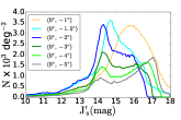
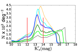
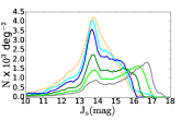
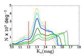
Appendix B MCMC results

Figures on the next page.

Figure 20: Parameter values for model $S$ as a function of iteration number for 10 walkers (each in a different colour) in the chain. All the walkers converge within the first 100 accepted steps to a value close to the starting point (green dotted line) chosen to be the result of the BFGS method (see Table 3, label ‘$\sigma^{\mathrm{RC}}$ free’).

Figure 21: One and two dimensional projections of the posterior probability distributions of the parameters of model $S$ (label ‘$\sigma^{\mathrm{RC}}$ free’ in Table 3), demonstrating the covariances between parameters. Along the diagonal, the 1-D marginalised distribution for each parameter is shown; on top of the distributions we give the 0.5 quantile values with the upper and lower errors (16% and 84% quantiles). For the initial state of the Markov chain we chose the best fit results reported in Table 3 (green dot). With 30,000 iterations and an acceptance fraction of 43%, the final results and errors on the parameters are in complete agreement with the values found using the BFGS method.

References

- Alcock et al. (2000) Alcock C., Allsman R. A., Alves D. R., Axelrod T. S. et al., 2000, ApJ, 541, 734
- Athanassoula (2005) Athanassoula E., 2005, MNRAS, 358, 1477
- Babusiaux & Gilmore (2005) Babusiaux C., Gilmore G., 2005, MNRAS, 358, 1309
- Benjamin et al. (2005) Benjamin R. A., Churchwell E., Babler B. L., Indebetouw R. et al., 2005, ApJ, 630, L149
- Binney et al. (1997) Binney J., Gerhard O., Spergel D., 1997, MNRAS, 288, 365
- Binney et al. (1991) Binney J., Gerhard O. E., Stark A. A., Bally J., Uchida K. I., 1991, MNRAS, 252, 210
- Bissantz & Gerhard (2002) Bissantz N., Gerhard O., 2002, MNRAS, 330, 591
- Blitz & Spergel (1991) Blitz L., Spergel D. N., 1991, ApJ, 379, 631
- Borissova et al. (2011) Borissova J., Bonatto C., Kurtev R., Clarke J. R. A. et al., 2011, A&A, 532, A131
- Bressan et al. (2012) Bressan A., Marigo P., Girardi L., Salasnich B., Dal Cero C., Rubele S., Nanni A., 2012, MNRAS, 427, 127
- Bruzual et al. (1997) Bruzual G., Barbuy B., Ortolani S., Bica E., Cuisinier F., Lejeune T., Schiavon R. P., 1997, AJ, 114, 1531
- Bureau et al. (2006) Bureau M., Aronica G., Athanassoula E., Dettmar R.-J., Bosma A., Freeman K. C., 2006, MNRAS, 370, 753
- Byrd et al. (1995) Byrd, R. H.and Lu P., Nocedal J., Zhu C., 1995, SIAM J. Sci. Comput., 16, 1190
- Calamida et al. (2015) Calamida A., Sahu K. C., Casertano S., Anderson J. et al., 2015, ApJ, 810, 8
- Cao et al. (2013) Cao L., Mao S., Nataf D., Rattenbury N. J., Gould A., 2013, MNRAS, 434, 595
- Catchpole et al. (2016) Catchpole R. M., Whitelock P. A., Feast M. W., Hughes S. M. G., Irwin M., Alard C., 2016, MNRAS, 455, 2216
- Chabrier (2003) Chabrier G., 2003, PASP, 115, 763
- Cole & Binney (2016) Cole D. R., Binney J., 2016, ArXiv e-prints
- Dékány et al. (2013) Dékány I., Minniti D., Catelan M., Zoccali M., Saito R. K., Hempel M., Gonzalez O. A., 2013, ApJ, 776, L19
- Dwek et al. (1995) Dwek E., Arendt R. G., Hauser M. G., Kelsall T. et al., 1995, ApJ, 445, 716
- Evans & Belokurov (2002) Evans N. W., Belokurov V., 2002, ApJ, 567, L119
- Foreman-Mackey et al. (2013) Foreman-Mackey D., Hogg D. W., Lang D., Goodman J., 2013, PASP, 125, 306
- Freudenreich (1998) Freudenreich H. T., 1998, ApJ, 492, 495
- Gerhard & Martinez-Valpuesta (2012) Gerhard O., Martinez-Valpuesta I., 2012, ApJ, 744, L8
- Girardi (2016) Girardi L., 2016, ARA&A, 54, 95
- Gonzalez et al. (2011) Gonzalez O. A., Rejkuba M., Minniti D., Zoccali M., Valenti E., Saito R. K., 2011, A&A, 534, L14
- Gonzalez et al. (2013) Gonzalez O. A., Rejkuba M., Zoccali M., Valent E., Minniti D., Tobar R., 2013, A&A, 552, A110
- Gonzalez et al. (2012a) Gonzalez O. A., Rejkuba M., Zoccali M., Valenti E., Minniti D., Schultheis M., Tobar R., Chen B., 2012a, A&A, 543, A13
- Gonzalez et al. (2012b) Gonzalez O. A., Rejkuba M., Zoccali M., Valenti E., Minniti D., Schultheis M., Tobar R., Chen B., 2012b, A&A, 543, A13
- González-Fernández et al. (2014) González-Fernández C., Asensio Ramos A., Garzón F., Cabrera-Lavers A., Hammersley P. L., 2014, ApJ, 782, 86
- Gran et al. (2016) Gran F., Minniti D., Saito R. K., Zoccali M. et al., 2016, ArXiv e-prints
- Hawkins et al. (2017) Hawkins K., Leistedt B., Bovy J., Hogg D. W., 2017, ArXiv e-prints
- Haywood et al. (2016) Haywood M., Di Matteo P., Snaith O., Calamida A., 2016, ArXiv e-prints
- Kormendy & Kennicutt (2004) Kormendy J., Kennicutt, Jr. R. C., 2004, ARA&A, 42, 603
- Kunder et al. (2016) Kunder A., Rich R. M., Koch A., Storm J. et al., 2016, ApJ, 821, L25
- Laney et al. (2012) Laney C. D., Joner M. D., Pietrzyński G., 2012, MNRAS, 419, 1637
- Li & Shen (2012) Li Z.-Y., Shen J., 2012, ApJ, 757, L7
- López-Corredoira (2016) López-Corredoira M., 2016, A&A, 593, A66
- López-Corredoira (2017) López-Corredoira M., 2017, ApJ, 836, 218
- López-Corredoira et al. (2000) López-Corredoira M., Hammersley P. L., Garzón F., Simonneau E., Mahoney T. J., 2000, MNRAS, 313, 392
- Marigo et al. (2008) Marigo P., Girardi L., Bressan A., Groenewegen M. A. T., Silva L., Granato G. L., 2008, A&A, 482, 883
- Marigo et al. (2017) Marigo P., Girardi L., Bressan A., Rosenfield P. et al., 2017, ApJ, 835, 77
- Martinez-Valpuesta et al. (2006) Martinez-Valpuesta I., Shlosman I., Heller C., 2006, ApJ, 637, 214
- McWilliam & Zoccali (2010) McWilliam A., Zoccali M., 2010, ApJ, 724, 1491
- Minniti et al. (2010) Minniti D., Lucas P. W., Emerson J. P., Saito R. K. et al., 2010, New Astronomy, 15, 433
- Nataf et al. (2010) Nataf D. M., Udalski A., Gould A., Fouqué P., Stanek K. Z., 2010, ApJ, 721, L28
- Nataf et al. (2015) Nataf D. M., Udalski A., Skowron J., Szymański M. K. et al., 2015, MNRAS, 447, 1535
- Ness et al. (2014) Ness M., Debattista V. P., Bensby T., Feltzing S., Roškar R., Cole D. R., Johnson J. A., Freeman K., 2014, ApJ, 787, L19
- Ness & Lang (2016) Ness M., Lang D., 2016, AJ, 152, 14
- Nikolaev & Weinberg (1997) Nikolaev S., Weinberg M. D., 1997, ApJ, 487, 885
- Nishiyama et al. (2005) Nishiyama S., Nagata T., Baba D., Haba Y. et al., 2005, ApJ, 621, L105
- Nishiyama et al. (2009) Nishiyama S., Tamura M., Hatano H., Kato D., Tanabé T., Sugitani K., Nagata T., 2009, ApJ, 696, 1407
- Paczyński & Stanek (1998) Paczyński B., Stanek K. Z., 1998, ApJ, 494, L219
- Percival & Salaris (2003) Percival S. M., Salaris M., 2003, MNRAS, 343, 539
- Pietrinferni et al. (2004) Pietrinferni A., Cassisi S., Salaris M., Castelli F., 2004, ApJ, 612, 168
- Pietrukowicz et al. (2015) Pietrukowicz P., Kozłowski S., Skowron J., Soszyński I. et al., 2015, ApJ, 811, 113
- Portail et al. (2015) Portail M., Wegg C., Gerhard O., Martinez-Valpuesta I., 2015, MNRAS, 448, 713
- Rattenbury et al. (2007) Rattenbury N. J., Mao S., Sumi T., Smith M. C., 2007, MNRAS, 378, 1064
- Robin et al. (2012) Robin A. C., Marshall D. J., Schultheis M., Reylé C., 2012, A&A, 538, A106
- Robin et al. (2003) Robin A. C., Reylé C., Derrière S., Picaud S., 2003, A&A, 409, 523
- Robin et al. (2014) Robin A. C., Reylé C., Fliri J., Czekaj M., Robert C. P., Martins A. M. M., 2014, A&A, 569, A13
- Rubele et al. (2012) Rubele S., Kerber L., Girardi L., Cioni M.-R. et al., 2012, A&A, 537, A106
- Saito et al. (2012) Saito R. K., Minniti D., Dias B., Hempel M. et al., 2012, A&A, 544, A147
- Saito et al. (2011) Saito R. K., Zoccali M., McWilliam A., Minniti D., Gonzalez O. A., Hill V., 2011, AJ, 142, 76
- Salpeter (1955) Salpeter E. E., 1955, ApJ, 121, 161
- Schultheis et al. (2014) Schultheis M., Zasowski G., Allende Prieto C., et al, 2014, AJ, 148, 24
- Sharma et al. (2011) Sharma S., Bland-Hawthorn J., Johnston K. V., Binney J., 2011, ApJ, 730, 3
- Sharma et al. (2016) Sharma S., Stello D., Bland-Hawthorn J., Huber D., Bedding T. R., 2016, ApJ, 822, 15
- Shen et al. (2010) Shen J., Rich R. M., Kormendy J., Howard C. D., De Propris R., Kunder A., 2010, ApJ, 720, L72
- Skrutskie et al. (2006) Skrutskie M. F., Cutri R. M., Stiening R., Weinberg M. D. et al., 2006, AJ, 131, 1163
- Stanek et al. (1994) Stanek K. Z., Mateo M., Udalski A., Szymanski M., Kaluzny J., Kubiak M., 1994, ApJ, 429, L73
- Stanek et al. (1997) Stanek K. Z., Udalski A., SzymaŃski M., KaŁuŻny J., Kubiak Z. M., Mateo M., KrzemiŃski W., 1997, ApJ, 477, 163
- Sumi et al. (2013) Sumi T., Bennett D. P., Bond I. A., Abe F. et al., 2013, ApJ, 778, 150
- Unavane & Gilmore (1998) Unavane M., Gilmore G., 1998, MNRAS, 295, 145
- Valenti et al. (2016) Valenti E., Zoccali M., Gonzalez O. A., Minniti D. et al., 2016, A&A, 587, L6
- Vallée (2017) Vallée J. P., 2017, Astrophysics and Space Science, 362, 79
- Vanhollebeke et al. (2009) Vanhollebeke E., Groenewegen M. A. T., Girardi L., 2009, A&A, 498, 95
- Wegg & Gerhard (2013) Wegg C., Gerhard O., 2013, MNRAS, 435, 1874
- Wegg et al. (2015) Wegg C., Gerhard O., Portail M., 2015, MNRAS, 450, 4050
- Zoccali et al. (2000) Zoccali M., Cassisi S., Frogel J. A., Gould A., Ortolani S., Renzini A., Rich R. M., Stephens A. W., 2000, ApJ, 530, 418
- Zoccali et al. (2008) Zoccali M., Hill V., Lecureur A., Barbuy B., Renzini A., Minniti D., Gómez A., Ortolani S., 2008, A&A, 486, 177
- Zoccali et al. (2003) Zoccali M., Renzini A., Ortolani S., Greggio L. et al., 2003, A&A, 399, 931
- Zoccali & Valenti (2016) Zoccali M., Valenti E., 2016, PASA, 33, e025
- Zoccali et al. (2017) Zoccali M., Vasquez S., Gonzalez O. A., Valenti E. et al., 2017, A&A, 599, A12