An observational method for fast stochastic X-ray polarimetry-timing

Abstract

The upcoming launch of the first space based X-ray polarimeter in $\sim 40$ years will provide powerful new diagnostic information to study accreting compact objects. In particular, analysis of rapid variability of the polarisation degree and angle will provide the opportunity to probe the relativistic motions of material in the strong gravitational fields close to the compact objects, and enable new methods to measure black hole and neutron star parameters. However, polarisation properties are measured in a statistical sense, and a statistically significant polarisation detection requires a fairly long exposure, even for the brightest objects. Therefore, the sub-minute timescales of interest are not accessible using a direct time-resolved analysis of polarisation degree and angle. Phase-folding can be used for coherent pulsations, but not for stochastic variability such as quasi-periodic oscillations. Here, we introduce a Fourier method that enables statistically robust detection of stochastic polarisation variability for arbitrarily short variability timescales. Our method is analogous to commonly used spectral-timing techniques. We find that it should be possible in the near future to detect the quasi-periodic swings in polarisation angle predicted by Lense-Thirring precession of the inner accretion flow. This is contingent on the mean polarisation degree of the source being greater than $\sim 4-5\%$, which is consistent with the best current constraints on Cygnus X-1 from the late 1970s.

1 Introduction

Accreting compact objects radiate brightly in X-rays, enabling a view of the region close to the horizon in the case of black holes (BHs), or the surface in the case of neutron stars (NSs). Accretion occurs through a geometrically thin disk, which emits a thermalised spectrum (Novikov & Thorne 1973; Shakura & Sunyaev 1973), and a hot cloud of electrons located close to the compact object, in which photons are Compton up-scattered into a cut-off power-law spectrum (Thorne & Price 1975; Eardley et al. 1975). The exact geometry of this electron cloud is still debated, with candidate models including evaporation of the inner disk into a large scale-height accretion flow (Eardley et al. 1975), the base of a jet (Markoff et al. 2005), and a coronal layer held above the disk by magnetic reconnection (Galeev et al. 1979; Haardt & Maraschi 1991). In the case of NSs, additional radiation is associated with the surface of the compact star.

Since the region of interest closest to the compact object cannot be directly imaged, the accretion geometry there can only be inferred by analysing the properties of the X-ray signal. For the past $\sim 40$ years this has been limited to analysis of the spectral and variability properties, with particular success resulting from combining the two disciplines (e.g. Miyamoto et al. 1988; Maccarone & Coppi 2002; Skipper et al. 2013). Such ‘spectral-timing’ techniques allow, for instance, analysis of propagating accretion rate fluctuations (e.g. Ingram & van der Klis 2013; Rapisarda et al. 2017) and reverberation mapping (e.g. Uttley et al. 2014). Soon with the (proposed late 2020) launch of the Imaging X-ray Polarimetry Explorer (IXPE: Weisskopf et al. 2016), it will also be possible, for the first time since OSO 8 was switched off in 1978, to observe the X-ray polarisation of these sources. Polarimetry provides two extra properties: the polarisation degree and angle. Analysis of these properties as a function of energy (spectral-polarimetry) will provide a powerful new lever arm to determine the geometry of the system and measure parameters of the compact object (e.g. Stark & Connors 1977; Schnittman & Krolik 2010; Dovčiak et al. 2011). Analysis of the rapid variability of the polarisation degree and angle will provide similarly powerful diagnostics. For instance, this will allow us to track propagation of accretion rate fluctuations from strongly to weakly polarised regions of the accretion flow and vice versa, and will provide a new way to disentangle scattered from directly observed photons for the purposes of reverberation mapping.

Accreting stellar-mass BHs and NSs display a rich phenomenology of X-ray variability properties on timescales ranging from milliseconds to hundreds of seconds (e.g. van der Klis 2006). In particular, quasi-periodic oscillations (QPOs) are often observed. These signals can be classified depending on the fundamental frequency of the oscillation. Low frequency (LF) QPOs are routinely observed from both BHs and NSs, often with a large amplitude. The observed frequency range for BHs is $\sim 0.1-30$ Hz, with the higher frequencies observed from NSs consistent with simple mass scaling (Wijnands et al. 1999; van der Klis 2005; Belloni 2010). BHs occasionally display high frequency (HF) QPOs, with frequencies $\gtrsim 100$ Hz (e.g. Morgan et al. 1997; Remillard et al. 1999; Homan et al. 2001). Even though these features are extremely rare and weak, they command significant theoretical interest because their frequencies are commensurate with the orbital frequency at the innermost stable circular orbit (Stella et al. 1999; Motta et al. 2014). NSs on the other hand display kHz QPOs which are common and often strong features (Strohmayer et al. 1996; van der Klis et al. 1996). Although it is tempting to interpret HF QPOs as the BH equivalent of kHz QPOs, this comparison is challenging on closer inspection (Motta et al. 2017).

All of these classes of QPO are often interpreted as a geometrical effect, giving rise to the possibility of detecting a QPO in the polarisation degree and/or angle with a sufficiently sensitive X-ray polarimeter. In particular, there is now mounting evidence that LF QPOs in BHs (or at least the ‘Type C’ subclass of LF QPOs; see e.g. Casella et al. 2005) result from Lense-Thirring precession of the inner accretion flow (Stella & Vietri 1998; Ingram et al. 2009). This is a relativistic effect in which a spinning compact object twists up the surrounding spacetime, inducing nodal precession in nearby orbits inclined to the BH equatorial plane (Lense & Thirring 1918). Ingram et al. (2016) recently discovered that the iron K$\alpha$ fluorescence line in the spectrum of the accreting BH H 1743$-$322 rocks from red to blue shifted over the course of a QPO cycle, confirming a distinctive prediction of the precession model (Schnittman et al. 2006; Ingram & Done 2012). This model also predicts a QPO in both the polarisation angle, resulting from the changing projected orientation of the accretion flow, and in polarisation degree, resulting from the expected angular dependence of Compton scattering (Ingram et al. 2015). Confirmation of these predictions would not only provide smoking gun evidence for the precession hypothesis, but would also provide tight geometrical constraints, particularly in combination with QPO phase-resolved iron line modeling (i.e. tomography: Ingram et al. 2017).

Detection of rapid variability of the polarisation degree and/or angle would therefore provide a valuable probe of these systems. However, the polarisation properties cannot be directly measured on arbitrarily short timescales due to Poisson counting statistics. For the count rates to be expected ($\sim$tens to hundreds of c/s), the polarisation properties cannot be constrained directly with sub-minute timescale resolution. Coherent pulsations can be studied simply by folding the light curve, but folding is not appropriate for stochastic variability (including QPOs; e.g. Ingram & van der Klis 2015). Here, we present a simple and robust general method for detecting rapid variability in X-ray polarisation properties, circumventing the technical challenges associated with stochastic variability. We focus our analysis mainly on QPOs, but the method can also be used for broad band variability. In Section 2, we present our method. In Section 3, we run simulations to determine the expected signal to noise of the QPOs in polarisation degree and angle predicted by the precession model. In Section 4, we analyse the improvement in signal to noise that can be achieved by cross correlating the polarimeter signal with a reference light curve collected with a large area X-ray detector, before summarising our results in Section 5.

2 The Method

In this Section, we first outline why a special method is required for fast X-ray polarimetry-timing before presenting our method.

Figure 1: Fractional variability amplitude (left) and phase lag (right) as a function of modulation angle, $\psi$, for the QPO fundamental frequency. The red solid lines assume the oscillations in flux, polarisation degree and polarisation angle calculated for the high inclination ($i=70^{\circ}$) model shown in Fig 6 of Ingram et al. (2015) (solid lines therein). The blue dashed lines result from assuming the same QPO in the flux, but constant polarisation degree and angle. Sinusoidal modulations such as those depicted by the red lines therefore provide a robust diagnostic of variability in polarisation properties. The black points are a simulation of a 200 ks IXPE exposure, assuming the red lines as the input model.

Figure 2: The same as for Fig. 1, except we now use as input the low inclination ($i=30^{\circ}$) model shown in Fig 8 of Ingram et al. (2015) (solid lines therein).

2.1 The Problem

We wish to detect fast ($<10$ s) variability of the polarisation degree $p_{0}$ and angle $\psi_{0}$. This is not trivial, since we measure these parameters in a statistical sense by detecting many photons. For each photon, a modulation angle, $\psi$, is measured, which is effectively an estimate for the instantaneous polarisation angle of the population of photons. For a photoelectric effect polarimeter such as the gas pixel detectors (GPDs) used on IXPE, this measurement of $\psi$ is obtained from the orientation of the electron tracks on the detector. Similar GPD detectors are also planned to be onboard the proposed missions The X-ray Imaging Polarimetry Explorer (XIPE; Soffitta et al. 2016) and the Extended X-ray Timing and Polarimetry mission (eXTP; Zhang et al. 2016). For a Thomson scattering polarimeter such as the balloon experiment X-Calibur (Guo et al. 2013), the measurement is instead obtained from the position on the detector where the photon lands. After enough photons have been collected, the polarisation properties can be measured from a histogram of photon counts versus modulation angle $\psi$. Specifically, the detected counts as a function of $\psi$ will be proportional to the modulation function

$$f(\psi|\psi_{0},p_{0},\mu)=\frac{1}{2\pi}\bigg{\{}1+\mu~{}p_{0}\cos[2(\psi_{0}-\psi)]\bigg{\}},$$ (1)

where $\mu$ is the modulation factor of the polarimeter, defined by the detector’s response to a $100\%$ polarised signal. Throughout this paper, we assume a modulation factor of $\mu=0.3$, which is expected for IXPE (Weisskopf et al. 2016). The polarisation degree $p_{0}$ can therefore be measured from the amplitude of the modulation function, and the polarisation angle $\psi_{0}$ can be measured from the location of the peak of the modulation function. Alternatively Stokes parameters can be used, which is essentially equivalent to measuring the shape of the modulation function. Note that the modulation function is cyclical on the interval $\psi=0$ to $\psi=180^{\circ}$, and therefore $\psi_{0}$ is only usefully defined on the interval $0$ to $180^{\circ}$ (or any interval spanning $180^{\circ}$). This is because a wave with a polarization angle of $\psi_{0}$ is indistinguishable from a wave with a polarization angle of $\psi_{0}+180^{\circ}$. For example, rotating a vertically polarised wave by $180^{\circ}$ leaves another vertically polarised wave. The modulation angle $\psi$, however, is defined on the interval $0$ to $360^{\circ}$ (or any interval spanning $360^{\circ}$). For photoelectric effect polarimeters, this is because the electron track caused by an incoming photon does have a direction since the starting point of the track can be determined, and $\psi$ is the angle between the electron track and the projection of north on the sky. For Thompson scattering polarimeters, $\psi$ also spans the full $360^{\circ}$ interval, since it is determined from the position on the detector where the photon is detected.

The simplest way to measure variability in $p_{0}$ and $\psi_{0}$ is of course to measure both properties directly for many time intervals. However, detection of polarisation requires a lot of photons. The minimum detectable polarisation (MDP) is the minimum polarisation degree that can be detected with statistical confidence $\mathcal{L}$. This is given by (Weisskopf et al. 2010)

$${\rm MDP}=\frac{-\ln(1-\mathcal{L})}{\mu\langle s\rangle}\sqrt{\frac{\langle s\rangle+\langle b\rangle}{T}},$$ (2)

where $\langle s\rangle$ and $\langle b\rangle$ represent mean source and background count rate respectively, and $T$ is the exposure time. Therefore, for a source with a mean polarisation degree of $\langle p_{0}\rangle=5\%$, a count rate of $\langle s\rangle=100$ c/s and a negligible background, achieving a statistical confidence of $\mathcal{L}=99\%$ requires a $T\approx 15$ minute exposure. For a higher intrinsic polarisation of $\langle p_{0}\rangle=10\%$, this is still $T\approx 4$ minutes. Therefore, with the expected count rates and reasonable assumptions about the polarisation degree, it is not possible to probe sub-minute timescales by directly calculating time series of $p_{0}$ and $\psi_{0}$. To probe faster timescales, we need a statistical method. For broad band variability and even QPOs, phase-folding is not a viable method. This is because the phase of the oscillation does not evolve with time in a predictable manner.

2.2 The Solution

We can instead consider the variability patterns that will be created in the modulation function from variability in the count rate, polarisation angle and polarisation degree. That is, we can make light curves selected by the modulation angle $\psi$ of each incoming photon, such that the count rate in the $i^{\rm th}$ $\psi$ bin at time $t$ is

$$s(\psi_{i},t)=s(t)f(\psi_{i}|\psi_{0}(t),p_{0}(t),\mu)\Delta\psi_{i},$$ (3)

where $\Delta\psi_{i}$ is the width of the $\psi$ bin, $s(t)$ is the total polarimeter count rate, and the modulation function, $f$, is given by Equation (1). From Equations (3) and (1), it is clear that, if only the total count rate is varying, and $p_{0}$ and $\psi_{0}$ are constant in time, then the light curves $s(\psi_{i},t)$ selected for each $\psi$ bin will all have the same fractional rms as one another, and will all vary in phase with one another. This is because the shape of the modulation function does not vary if $p_{0}$ and $\psi_{0}$ remain constant. In contrast, if only $p_{0}$ is varying (with $s$ and $\psi_{0}$ now constant), this will cause a stretching and squeezing of the modulation function as $p_{0}$ respectively increases and decreases. This will lead to a peak in fractional rms at $\psi=\psi_{0}$ and a minimum at $\psi=\psi_{0}+90^{\circ}$, with all the light curves varying in phase with one another as in the previous example. Finally, if we imagine only $\psi_{0}$ is varying (with $s$ and $p_{0}$ constant), the resulting rocking of the distribution peak will lead to light curves for $\psi_{i}>\langle\psi_{0}\rangle$ varying in anti-phase with light curves for $\psi_{i}<\langle\psi_{0}\rangle$. For a more general (and realistic) situation, with $s$, $p_{0}$ and $\psi_{0}$ all varying, an intuition is harder to form and calculations are required. However, it is possible to appreciate that variability of polarisation properties is encoded in the $\psi$ dependent variability properties of the signal, which can be probed using standard cross-spectral techniques developed for the purposes of spectral-timing.

We can therefore define a reference time series, $r(t)$, that is highly correlated with all the $s(\psi_{i},t)$ light curves and define a set of cross-spectra

$$C(\psi_{i},\nu,\Delta)=\langle S(\psi_{i},\nu)R^{*}(\nu)\rangle,$$ (4)

where an uppercase letter represents the Fourier transform (FT) of the corresponding lowercase letter and a star denotes a complex conjugate. The angle brackets denote averaging, which is over an ensemble of different realisations (i.e. the light curves are split into many segments) and also over the Fourier frequency range $\nu-\Delta/2$ to $\nu+\Delta/2$ (van der Klis et al. 1987). We see that the only difference with more familiar spectral-timing analyses, is that we are selecting light curves based on modulation angle rather than energy. Everything else is, in principle, entirely equivalent. The reference light curve may be provided by a second detector on the same satellite as the polarimeter, such as the $\sim 3{\rm m}^{2}$ Large Area Detector (LAD) of eXTP. Alternatively, it could be provided by a simultaneous pointing from another observatory, such as AstroSat (Singh et al. 2014) which is likely to still be in operation during the IXPE mission lifetime, or The Spectroscopic Time-Resolving Observatory for Broadband Energy X-rays (STROBE-X; Wilson-Hodge et al. 2017) which is proposed to include an $\sim 8{\rm m}^{2}$ version of the LAD. In the absence of another instrument, the total polarimeter count rate (i.e. summed over all $\psi$) could be used. It is convenient if the reference time series is statistically independent from the other light curves. This property is automatically satisfied by the use of a second instrument, and can be ensured by using, for example, the total polarimeter count rate minus the currently considered $\psi$ bin in the absence of a second instrument (in direct analogy to spectral-timing techniques; e.g. Uttley et al. 2014). From the cross-spectrum for a given Fourier frequency range, we can calculate the fractional rms as a function of $\psi$, and also the phase lag as a function of $\psi$ with respect to the reference time series (See Appendix A for more details).

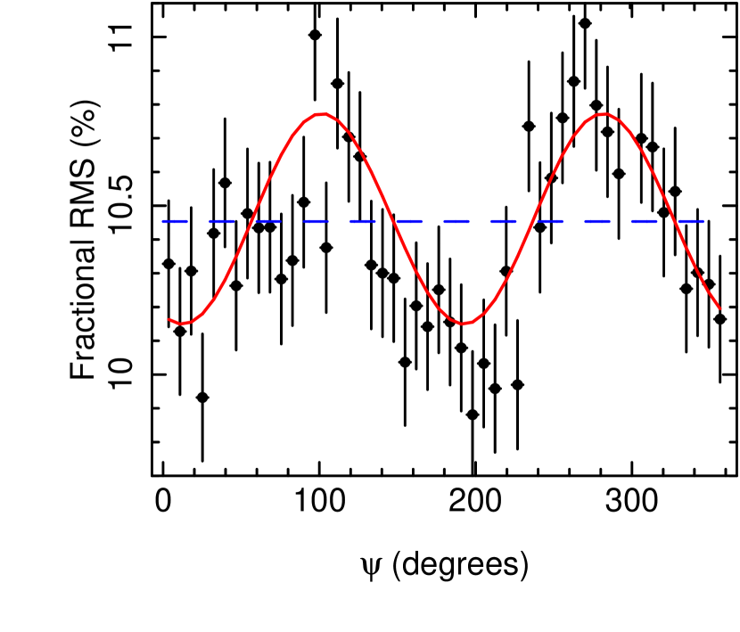
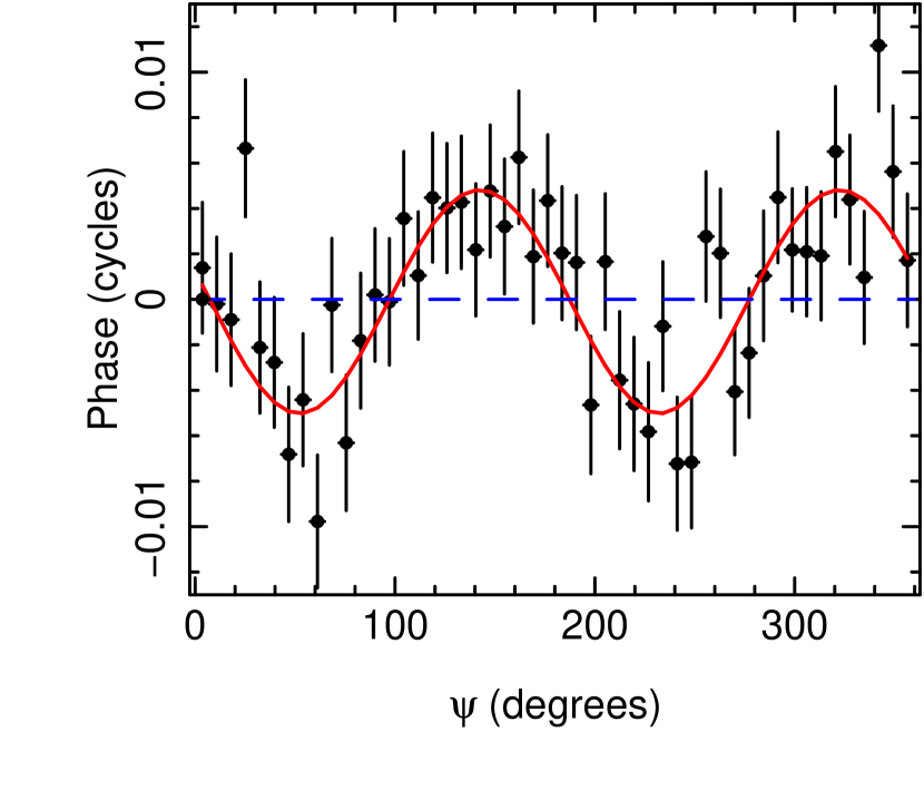
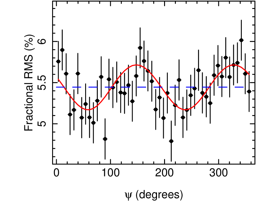
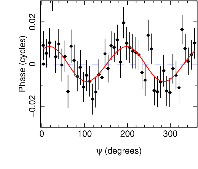
The red solid lines in Fig 1 and 2 show the fractional rms and phase lags as a function of $\psi$ calculated by inputing the (LF) QPOs in polarimeter count rate, polarisation degree and angle predicted by Ingram et al. (2015). In that paper, the authors ray trace radiation from a precessing torus to a distant observer using the Kerr metric, and calculate the resulting polarisation properties as a function of precession phase. Two parameter combinations are featured, referred to here as the high inclination model ($i=70^{\circ}$, $\Phi=110^{\circ}$, $\beta=10^{\circ}$; see Fig 6 in Ingram et al. 2015) and the low inclination model ($i=30^{\circ}$, $\Phi=180^{\circ}$, $\beta=10^{\circ}$; see Fig 8 in Ingram et al. 2015). Note that Ingram et al. (2015) used the symbol $\chi$ for the polarisation angle, whereas here we use the symbol $\psi_{0}$ - reserving $\chi$ for the $\chi^{2}$ fit statistic. Figs 1 and 2 correspond to the high and low inclination model respectively. We consider the rms and phase lags at the QPO fundamental frequency, and we also take onto account the broad band noise that is observed coincident with Type C QPOs. The details of our calculation are presented in Appendix A. The figures show approximately sinusoidal modulations in both the amplitude and phase resulting from $p_{0}$ and $\psi_{0}$ varying with QPO phase. The blue dashed lines show an alternative, null-hypothesis, model, in which only the count rate varies and $p_{0}$ and $\psi_{0}$ stay constant with QPO phase. As expected, we see no modulations in either the amplitude or phase for this null-hypothesis model. We therefore have a simple and statistically robust way to detect variability in the polarisation properties: simply by looking for these $\sim$sinusoidal modulations in the rms and phase lags as a function of $\psi$. We note that just detecting these modulations does not automatically tell us about whether it is $p_{0}$, $\psi_{0}$ or both varying. This requires a more detailed analysis (see Section 3.3). There is one exception however. If $\psi_{0}$ is constant and $p_{0}$ varies in phase with the total count rate, then there will be a sinusoidal modulation in the amplitude but not in the phase lags. We finally note that the rms and phase are both cyclical on the interval $0$ to $180^{\circ}$, which is because $\psi_{0}$ is only defined on an interval of $180^{\circ}$ (see Section 2.1).

3 Simulations

In this section, we present methods to detect $p_{0}$ and $\psi_{0}$ oscillations in noisy data, with null-hypothesis significance testing. Throughout, we consider a $200$ ks exposure of a bright source (absorbed power-law spectrum with index $\Gamma=2$, normalisation $=3$ photons/s/cm²/keV, hydrogen column density $n_{h}=10^{22}$ cm^-1) with negligible background, comparable to e.g. GX 339-4 in a bright hard state or intermediate state. We first describe our simulation method, focusing on IXPE. We then introduce a simple null-hypothesis test, which compares a sinusoidal model for the rms and phase lag modulations as a function of $\psi$ to a null-hypothesis model with constant rms and phase lag. This determines the statistical confidence with which we prefer a model with variable polarisation properties over a null-hypothesis model with constant polarisation properties. We then specifically consider how to constrain an oscillation in polarisation angle, which is the most interesting quantity, offering a ‘smoking gun’ detection of precession.

The null-hypothesis tests presented here additionally allow us to properly explore trade-offs when deciding whether to target high or low inclination sources to search for an oscillation in polarisation angle. In the precession model (and in the observational data: Schnittman et al. 2006; Motta et al. 2015; Heil et al. 2015), the oscillation in the flux has a larger amplitude for higher inclinations (i.e. systems viewed more edge-on), since there is more variability in solid angle and Doppler boosting over each precession cycle. The mean polarisation degree is also expected to increase with inclination angle (Chandrasekhar 1960; Sunyaev & Titarchuk 1985). However, the oscillation in polarisation angle has a greater amplitude for the low inclination model, since a precessing vector traces out a cone when viewed from the side and a full circle when viewed from the top. We therefore consider both the high and low inclination model in this Section.

3.1 Simulation setup

We present details of our simulations in Appendix B. Here we summarise the general scheme. We calculate our model for the fractional rms and phase lag corresponding to each QPO harmonic as a function of $\psi$ as described in Appendix A. We generate synthetic data by calculating $1~{}\sigma$ errors on the model (the expression for which we present and discuss in Appendix B) and selecting Gaussian random variables. With real data, we would measure the rms and phase lags by calculating the cross-spectrum for many segments, each of length $T_{\rm seg}$ seconds, and averaging. We would also average over all the frequency bins lying in the frequency range $\Delta$ Hz. Since there are a total of $T/T_{\rm seg}$ segments (where $T$ is the total exposure time), and the frequency resolution is $d\nu=1/T_{\rm seg}$ (van der Klis 1989), the averaging is over $T\Delta$ realisations of the cross-spectrum. Therefore $T$ and $\Delta$ are important parameters for calculating the error on the rms and phase lags. For a QPO, it is appropriate to average over the frequency range $\nu_{k}-\Delta_{k}/2$ to $\nu_{k}+\Delta_{k}/2$, where $\nu_{k}$ and $\Delta_{k}$ are respectively the centroid frequency and full width at half maximum (FWHM) of the $k^{\rm th}$ QPO harmonic. These two parameters are related by the quality factor, $Q=\nu_{k}/\Delta_{k}$, which is generally observed to be $Q\sim 8-10$ for most Type C LF QPOs (note that the quality factor is generally equal for all detected harmonics). The remaining inputs required to calculate the errors are the mean polarimeter and reference time series count rates, $\langle s\rangle$ and $\langle r\rangle$. These parameters determine the Poisson noise level.

The black points in Fig 1 and 2 show our simulation results for a $T=200$ ks simulated exposure with only IXPE, using the red solid lines as the input model. The polarimeter mean count rate is $\langle s\rangle=100$ c/s, calculated assuming the spectral parameters defined at the start of this Section and folding around the IXPE response matrix. We set the reference time series count rate to $\langle r\rangle=\langle s\rangle$, assuming that we can use the total IXPE count rate as the reference time series. We set $\Delta=0.2$ Hz, which is appropriate for a QPO with centroid frequency $\nu=1.6$ Hz and quality factor $Q=8$. For the high inclination model (Fig 1), the predicted modulations in both fractional rms and phase lag are clearly visible. For the low inclination model (Fig 2), the modulations are less clear in the rms, but can be seen in the larger amplitude phase lag modulations (resulting from the larger amplitude oscillations in polarisation angle in the low inclination model). We only plot the results for the QPO fundamental here. The modulations are not detectable in the synthetic data for higher harmonics.

3.2 Null-hypothesis testing

We now formally test the confidence with which we can rule out a null-hypothesis of constant $p_{0}$ and $\psi_{0}$ for the synthetic data points in Fig 1 and 2. For this null-hypothesis, the fractional rms and phase would not depend on $\psi$. Alternatively, for a model in which $p_{0}$ and/or $\psi_{0}$ are varying, the fractional rms and phase would have an approximately sinusoidal dependence on $\psi$. We can therefore fit two models to the data and, since one model is a ‘nested’ version of the other, compare the goodness of fit using an F-test. For the null-hypothesis, we simply calculate the error weighted mean fractional amplitude and phase lag from the data (this is identical finding a best-fitting constant by minimising $\chi^{2}$). For the ‘full’ model, we fit a sinusoid function to both fractional rms and phase lag

$$y(\psi)=A+B\cos[2(\psi-C)],$$ (5)

where $A$, $B$ and $C$ are free parameters in each of the two fits (i.e. one fit to the rms and the other to the lags).

For the high inclination simulation shown in Fig 1, the best fitting null-hypothesis model has a reduced $\chi^{2}$ of $\chi^{2}_{\nu}=234.6/98$. This is calculated for both rms and phase over a total of 100 data points (50 rms points and 50 lag points), with only two free parameters (the mean rms and the mean phase lag), resulting in 98 degrees of freedom. The sinusoidal model has a much better reduced $\chi^{2}$ of $98.6/94$. Here, there are the same number of data points but now there are 6 free parameters ($A$, $B$ and $C$ for rms and phase lag), giving 94 degrees of freedom. An F-test returns an F statistic of $F=32.4$, which corresponds to a null-hypothesis p-value far lower than the threshold for $5\sigma$ confidence ($p=6\times 10^{-17}$). For the low inclination simulation shown in Fig 2, the reduced $\chi^{2}$ values for null-hypothesis and sinusoidal models are instead $\chi^{2}_{\nu}=158.2/98$ and $\chi^{2}_{\nu}=85.8/94$ respectively. This again gives a p-value corresponding to $>5\sigma$ confidence ($F=19.8$, $p=7\times 10^{-12}$). As a final check, we also compare the input model with the data, to get $\chi^{2}_{\nu}=104.9/100$ and $\chi^{2}_{\nu}=90.0/100$ for the high and low inclination models respectively, indicating good fits.

We note that $\chi^{2}$ statistics are only appropriate for the case of Gaussian errors. This is clearly the case for our simulation, since we select Gaussian random variables. In practice however, the cross-spectra must be averaged over a suitably large number of realisations for the Gaussian limit to be reached (i.e. the central limit theorem). This requires $T\Delta\gtrsim 400$ (Vaughan et al. 2003), which is comfortably the case for our chosen parameters ($T\Delta=2\times 10^{4}$).

Thus, we expect to be able to detect the oscillations predicted by Ingram et al. (2015), even for low inclination sources. However, there is of course some uncertainty over what we expect theoretically for the $p_{0}$ and $\psi_{0}$ oscillations. It is therefore worth exploring parameter space with our new simple hypothesis testing tool. The most robust prediction of the precession model is the $\psi_{0}$ oscillation, since this largely depends on geometry alone. The modulation in $p_{0}$ is much more uncertain, since it depends on the angular dependence of emergent radiation, which in turn depends on the details of the Comptonisation process that drives the hard X-ray radiation. A key uncertainty is the average polarisation degree, $\langle p_{0}\rangle$. In particular, the calculations of Sunyaev & Titarchuk (1985) used by Ingram et al. (2015) may over-estimate $\langle p_{0}\rangle$, since they only consider photons that have had ‘many scatterings’. More detailed calculations have since predicted lower polarisation from Comptonisation (e.g. Schnittman & Krolik 2010), particularly in the $2-8$ keV range that the GPD detectors are sensitive to. This is largely because photons with energies of $2-8$ keV often do not fulfil the aforementioned criterion of having been scattered many times. It is worth mentioning that polarimeters sensitive to harder X-rays are therefore desirable, since more $\sim 10-50$ keV photons will have undergone many scatterings and are therefore expected to be more highly polarised (also the LF QPO fractional amplitude is often observed to increase with energy). Thomson scattering polarimeters such as the Polarization Spectroscopic Telescope Array (PolSTAR: Krawczynski et al. 2016), the proposed satellite version of X-Callibur, are therefore promising prospects for the future.

Figure 3: The curves show the $F$ statistic calculated by comparing the best-fitting sinusoid model with a null-hypothesis corresponding to constant polarisation properties (see text for further details) as a function of mean polarisation degree. The left and right plots are for the simulations corresponding to the high and low inclination models respectively. Each curve represents a different combination of mean count rate in the polarimeter $\langle s\rangle$ and mean count rate in the reference time series, $\langle r\rangle$. From bottom to top, they represent $\langle s\rangle=100$ c/s, $\langle r\rangle=100$ c/s (black solid), $\langle s\rangle=100$, $\langle r\rangle=5000$ (red dashed), $\langle s\rangle=200$, $\langle r\rangle=38,000$ (green dot-dashed) and $\langle s\rangle=500$, $\langle r\rangle=38,000$ (blue dotted). These cases are respectively relevant for IXPE alone, IXPE+AstroSat, eXTP baseline and eXTP goal. The grey dashed lines show $3\sigma$ and $5\sigma$ values. We see that, for the high inclination model, a $5\sigma$ detection is possible for $\langle p_{0}\rangle\gtrsim 5.5\%$ with IXPE alone, or $\langle p_{0}\rangle\gtrsim 2.3\%$ with the eXTP goal configuration. Smaller polarisation degrees are required for the low inclination model, but we do expect low inclination sources to be less polarised.

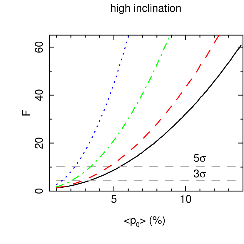
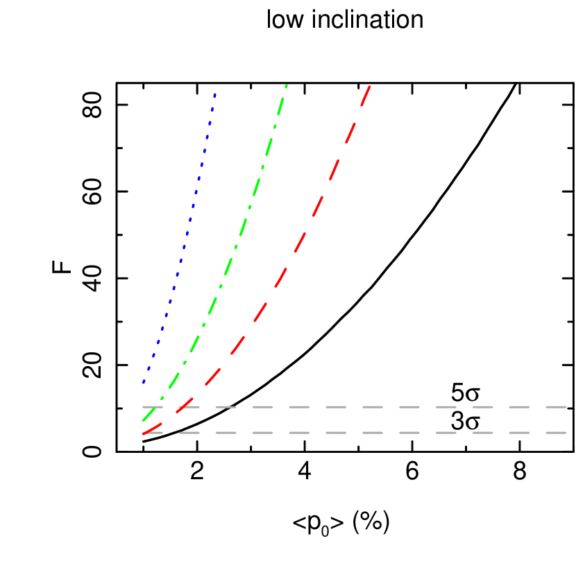
In Fig. 3, we therefore explore a range of $\langle p_{0}\rangle$ values, again considering a $200$ ks exposure and $\Delta=0.2$ Hz. We use the same high (left) and (low) inclination input models as before for $s$, $p_{0}$ and $\psi_{0}$ as a function of QPO phase, except we re-scale the $p_{0}$ oscillation by the new mean. The curves show the $F$ statistic resulting from comparing a null-hypothesis and a sinusoidal model to synthetic data for different polarimeter and reference time series count rates. In order to smooth out noise, we average $\chi^{2}$ values over $10,000$ realisations of synthetic data before doing the F-test. From bottom to top, the curves represent: only IXPE (black solid), IXPE with AstroSat recording the reference time series (red dashed), eXTP ‘requirement’ specifications with the reference time series recorded by the $\sim 3$ m² LAD (green dot-dashed) , and eXTP ‘goal’ specifications (blue dotted). The grey dashed lines represent $3$ and $5~{}\sigma$ confidence. As expected, the oscillations in $p_{0}$ and $\psi_{0}$ are harder to detect when the mean polarisation degree is low. Also, for lower inclination angles, the minimum degree of polarisation required for a significant detection of polarisation variability is smaller. This is because the swings in polarisation angle are predicted to have a larger amplitude for the low inclination model. However, we do expect a lower mean polarisation degree for lower inclinations, so it is likely still best to target high inclination sources. We see that sensitivity is improved by using configurations that increase the mean polarimeter count rate $\langle s\rangle$ and the mean reference time series count rate $\langle r\rangle$. Therefore, for a given polarimeter, we can increase signal to noise simply by observing simultaneously with another observatory with greater collecting area than the polarimeter. We will discuss the relative importance of high reference and polarimeter count rates in Section 4.

3.3 Measuring an oscillation in polarisation angle

Figure 4: Plot of minimum $\chi^{2}$ against the parameter $A_{1\psi}$ (black solid line) for fits to synthesised IXPE data. A non-zero value of this parameter indicates that the polarisation angle is modulated on the QPO fundamental. The left and right hand panels correspond to the high and low inclination models respectively. The red crosses show the input value of $A_{1\psi}$ for each simulation and the blue dashed lines show the $5\sigma$ confidence contour. For both input models the null-hypothesis of $A_{1\psi}=0$ can be strongly ruled out.

We have shown that it is simple to measure variability in polarisation properties with an X-ray polarimeter. However, determining if specifically the polarisation angle is oscillating, and/or if the polarisation degree is oscillating, and moreover measuring the amplitude and phase of those oscillations, requires further work. In this section, we show that a method entirely analogous to the Ingram et al. (2016) QPO phase-resolving method can be employed to do just this. We start by representing the oscillations in count rate, polarisation degree and angle as a simple phenomenological function of QPO phase, $\omega$. For example, the $\psi_{0}$ oscillation is given by

$$\psi_{0}(\omega)=\langle\psi_{0}\rangle+A_{1\psi_{0}}\sin[\omega-\phi_{1\psi_{0}}]+A_{2\psi_{0}}\sin[2(\omega-\phi_{2\psi_{0}})],$$ (6)

and we use equivalent expressions for $p_{0}(\omega)$ and $s(\omega)$. This is simply a sum of harmonics, where we only consider two harmonics (since in most cases only two QPO harmonics can be detected). Here, $A_{1\psi_{0}}$ and $A_{2\psi_{0}}$ are the amplitudes of respectively the first and second harmonics of the $\psi_{0}$ oscillation, and $\phi_{1\psi_{0}}$ and $\phi_{2\psi_{0}}$ are the phases. Including the 3 mean parameters ($\langle s\rangle$, $\langle p_{0}\rangle$ and $\langle\psi_{0}\rangle$), 6 amplitude parameters [i.e. $A_{1\psi_{0}}$, $A_{2\psi_{0}}$ and the equivalents for $p_{0}(\omega)$ and $s(\omega)$], and 6 phase parameters, there are 15 model parameters altogether. We simultaneously fit this model to the synthetic data of the mean count rate vs $\psi$, the fractional rms vs $\psi$ for two QPO harmonics, and the phase lag vs $\psi$ for two QPO harmonics. The simultaneous fit is therefore performed over a total of five datasets. We use xspec v 12.9 (Arnaud 1996).

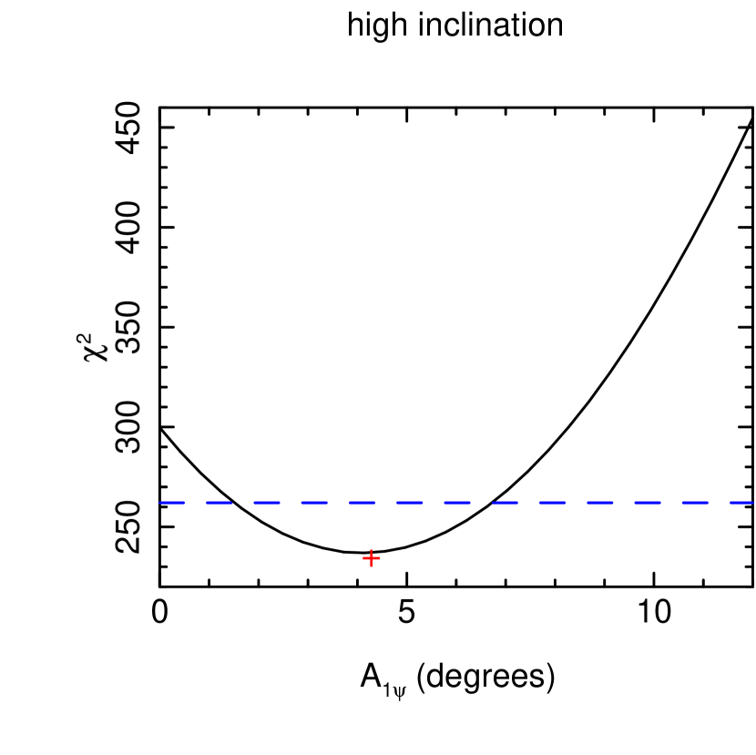
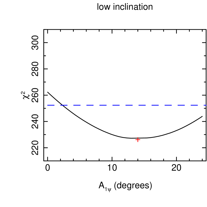
We use the same two simulations shown in Figs. 1 and 2. Although these figures only show the rms and phase for the QPO fundamental (i.e. first harmonic), we also consider the second harmonic and the mean count rate in our fit. Even though the synthetic data for the second harmonic are very noisy, they still constrain our model since they rule out parameter combinations that predict very large rms and lag modulations in the second harmonic that are not present in the synthetic data. Fig. 4 shows the minimum $\chi^{2}$ as a function of the parameter $A_{1\psi_{0}}$ (black solid line) for the high (left) and low (right) inclination models. In both cases, the red cross depicts the exact answer calculated directly from the input model for the simulation, which is clearly consistent with the best fit value. The blue dashed line depicts the $5~{}\sigma$ confidence contour. We see that the QPO in $\psi_{0}$ is detected with $>5\sigma$ confidence in both cases, with the significance being greater for the high inclination model. We note that the simulation includes the effect of broad band noise, but our simple model fitting in this Section does not. The fact that we recover the input polarisation angle oscillation accurately gives us confidence that the method is fairly robust to biases introduced by the broad band noise signal. Clearly, it is also possible to use the same method presented here to measure the oscillation in polarisation degree.

Figure 5: Mean polarisation degree required in order to make a $5\sigma$ detection of the oscillations in polarisation properties predicted by Ingram et al. (2015) for a high (left) and low (right) inclination object, plotted against mean count rate of the reference time series. We assume a 200 ks exposure and consider three different specifications of polarimeter, assuming mean polarimeter count rates of $\langle s\rangle=100$ c/s (black: IXPE), $\langle s\rangle=200$ c/s (red: XIPE / eXTP baseline) and $\langle s\rangle=500$ c/s (blue: eXTP goal). We see that increasing the polarimeter count rate increases sensitivity, as does increasing the reference count rate. We can therefore increase the sensitivity of a given polarimeter by using a large area instrument to collect the reference time series. There is however a saturation point (here at $\sim 5000$ c/s) beyond which increasing the reference count rate provides no further advantage.

Figure 6: Square of the 1 $\sigma$ error on the phase lag (in radians) between a $\psi$ bin with a count rate of 3 c/s and a reference time series, plotted against the count rate of the reference time series, $\langle r\rangle$. The magenta solid line depicts the total error and the other lines in the left hand plot show the 4 separate terms in the formula for the error (see Equation 7). The right hand plot is a zoom in of the left. The grey dashed vertical line depicts the ‘saturation count rate’ at which the error transitions from a very steep function of $\langle r\rangle$ to a more shallow dependence (see Equation 8).

4 The importance of a high count rate reference time series

It is clear from Fig. 3 that the reference count rate is important for detection. In this Section we explore the importance of the reference time series count rate, to assess how much of an advantage can be gained simply by using an instrument with higher effective area than the polarimeter to collect the reference time series. We first note that the most important property of the reference time series is that it is highly correlated with the polarimeter light curve. This is guaranteed if instruments with a similar spectral response are used to measure the polarimeter and reference time series. Therefore, instruments sensitive to the same $\sim 2-8$ keV band as the GPDs, such as the Neutron star Interior Composition ExploreR (NICER: Gendreau et al. 2016), the X-Ray Concentrator Array (XRCA) of STROBE-X and the Spectroscopic Focusing Array (SFA) of eXTP will provide an advantage in this respect. In practice though, hard and soft X-rays tend to be highly correlated for the case of accreting compact objects (e.g. Nowak et al. 1999), and so the harder response of the LAD is unlikely to be a problem. We therefore assume unity coherence throughout this paper.

4.1 The polarisation degree required for detection

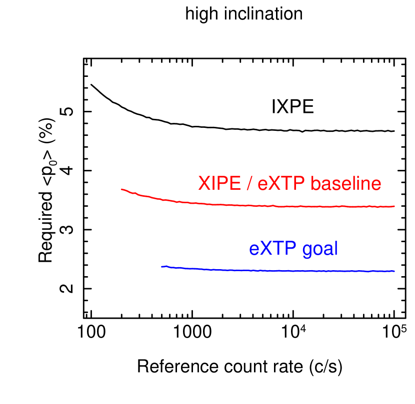
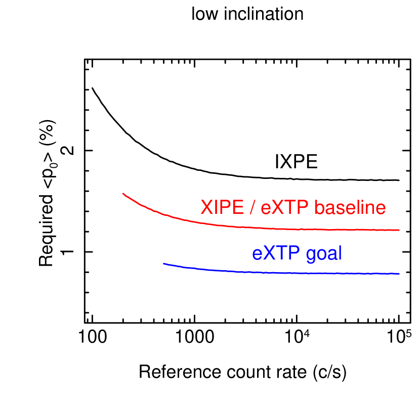
Fig 5 shows the mean polarisation degree required to detect polarisation variability with $5\sigma$ confidence plotted against mean reference time series count rate. Again, results for the high and low inclination models are plotted on the left and right respectively. To calculate the ‘detection polarisation degree’, $p_{\rm det}$, plotted on the y-axis, we find the $\langle p_{0}\rangle$ value for which the $F$ statistic for the simulation corresponds to $5\sigma$ confidence. For example, the solid black line in Fig 3 (left), representing $\langle s\rangle=\langle r\rangle=100$ c/s, crosses the $5\sigma$ level (upper dashed line) for $\langle p_{0}\rangle\approx 5.5\%$. Therefore, $p_{\rm det}\approx 5.5\%$ for IXPE ($\langle s\rangle=100$ c/s) when the reference time series mean count rate is $\langle r\rangle=100$ c/s.

We show results for three different polarimeters: IXPE (black), XIPE (which is the same as the baseline eXTP polarimeter; red) and eXTP goal (blue). For each line, we only consider $\langle r\rangle\geq\langle s\rangle$, since in practice there is no need to use a reference time series with a lower mean count rate than can be provided by the polarimeter itself. We again assume a $200$ ks exposure. We see that increasing the area of the polarimeter (from IXPE to XIPE to eXTP goal) has a large impact on sensitivity. Increasing the reference count rate also has a significant effect up until $\sim 5000$ c/s where the sensitivity starts to saturate. This is interesting, since AstroSat can achieve count rates of $\sim 5000$ c/s for a bright source as specified at the start of Section 3. Therefore, for the simulation parameters considered, AstroSat would perform comparably to the eXTP or STROBE-X versions of the LAD over a 200 ks exposure (that is, if the coherence between the LAD and GPD energy bands is high as assumed, otherwise NICER or the XRCA of STROBE-X may provide an advantage). We show below, however, that there are other parameter combinations for which the LAD gives a large advantage. It is also important to note that a $200$ ks exposure on a low Earth orbit satellite will take $\sim 5$ days to collect, over which time the QPO frequency will change fairly significantly. This would therefore need to be accounted for in the analysis [e.g. using techniques similar to the Méndez et al. (1998) ‘shift and add’ technique employed for kHz QPOs, or the Tomsick & Kaaret (2001) ‘stretch and bin’ technique employed for LF QPOs]. Finally, the detection polarisation degree is related very simply to the modulation factor, $\mu$. Doubling $\mu$ would half $p_{\rm det}$, and so polarimeter designs with larger $\mu$ are unsurprisingly more sensitive.

4.2 The ‘saturation count rate’

We can further understand the role of the reference time series by exploring the error on the phase lag. From Equation 17, the squared error is

$$\left[d\phi(\psi_{i},\nu)\right]^{2}\propto 1+\frac{P_{\rm noise}(\psi_{i})}{P(\psi_{i},\nu)}+\frac{P_{\rm noise}}{P(\nu)}+\frac{P_{\rm noise}P_{\rm noise}(\psi_{i})}{P(\nu)P(\psi_{i},\nu)}.$$ (7)

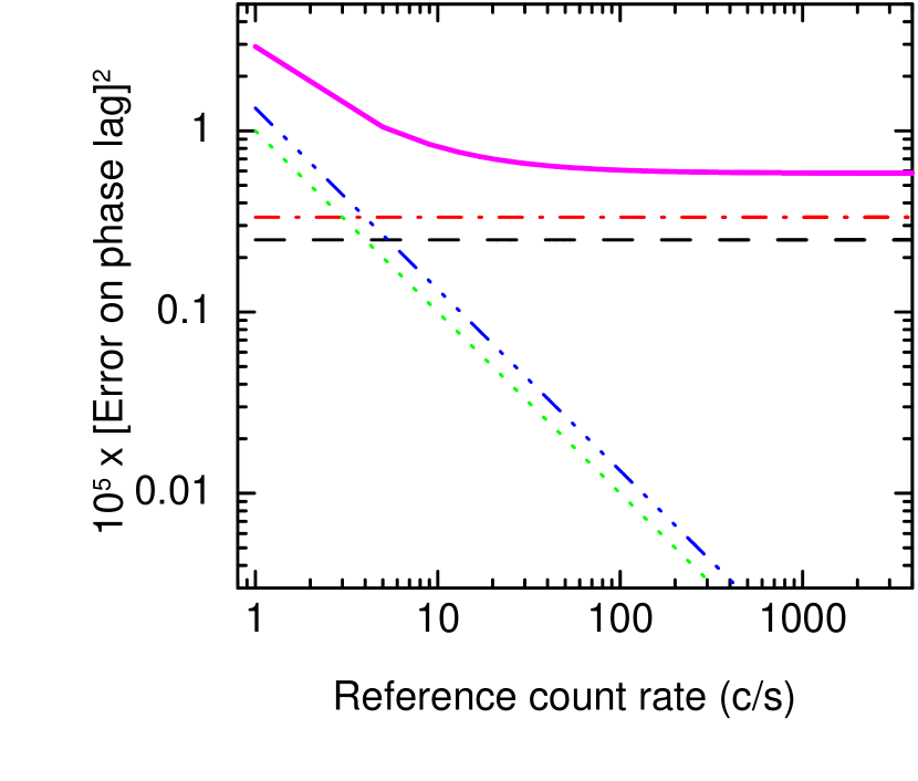
Here, $P(\nu)$ and $P(\psi_{i}\nu)$ are respectively the intrinsic (i.e. no Poisson noise) power spectra of the reference time series and the light curve for the $i^{\rm th}$ $\psi$ bin. $P_{\rm noise}$ and $P_{\rm noise}(\psi_{i})$ are respectively the Poisson noise contribution for the reference time series and the light curve for the $i^{\rm th}$ $\psi$ bin. Fig. 6 (left) shows this squared error for a $\psi$ bin with mean count rate $3$ c/s, as a function of reference band count rate, $\langle r\rangle$. We assume a QPO with $10\%$ fractional rms (consistent with the high inclination model), $T=200$ ks and $\Delta=0.2$ Hz. The solid magenta line shows the total, whereas the black dashed line, the red dot-dashed line, the green dotted line and the blue triple dot dashed line depict respectively the first, second, third and fourth terms on the right hand side of Equation 7. We see that the first two terms do not depend on $\langle r\rangle$, whereas the third and fourth terms reduce with $\langle r\rangle$. We also see that the second and fourth terms dominate over the others for this example, which turns out to be generally the case for the set of observed LF QPO properties.

Therefore, in the regime in which the fourth term dominates, we gain an enormous advantage by increasing the area used to collect our reference time series. If instead the second term dominates, any further increase in $\langle r\rangle$ gives a more incremental improvement. We can estimate this ‘saturation count rate’ by setting the second and fourth terms equal to one another to obtain

$$r_{\rm sat}=\frac{2(1+\langle b\rangle/\langle s\rangle)\Delta}{{\rm rms}^{2}},$$ (8)

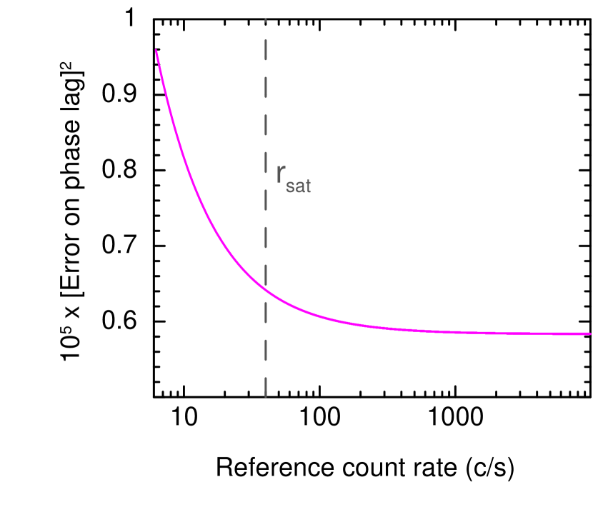
where $\langle b\rangle/\langle s\rangle$ is the fractional contribution of the polarimeter background (in this discussion we only consider $b=0$). We see that $r_{\rm sat}=40$ c/s for the parameters used in Fig. 6. It is important to note that $r_{\rm sat}$ marks only a change in regime. It is still possible to get an improvement in signal to noise by increasing $\langle r\rangle$, even for $\langle r\rangle>r_{\rm sat}$. Fig 6 (right) - a zoom in of Fig 6 (left) - demonstrates this. The error is still decreasing for $\langle r\rangle>r_{\rm sat}$ (grey dashed line), until $\langle r\rangle>>r_{\rm sat}$. We also see this in Fig 5, where the sensitivity still improves until $\langle r\rangle\sim 5000$ c/s, even though the saturation count rate is $r_{\rm sat}=40$ c/s.

Nonetheless, Equation 8 shows that a high count rate reference time series is most important for low rms, high $\Delta$ QPOs. Since LF QPOs have a roughly constant quality factor of $Q\sim 8$, high $\Delta$ translates to high $\nu_{qpo}$. Therefore, if we wish to observe QPOs with IXPE alone, we should target the lowest frequency, highest rms QPOs. For a fractional rms of $10\%$, we calculate that this transition in regime occurs at $\nu_{qpo}\sim 4$ Hz (by setting $r_{\rm sat}=100$ c/s, since this is the count rate achievable by IXPE alone).

For $\nu_{qpo}\gtrsim 4$ Hz a high count rate reference time series will vastly improve signal to noise, much more so than shown in Fig. 5. We do however need to keep in mind time lost to lining up orbits of two observatories, except for eXTP, which has both the polarimeter and the LAD onboard. It is clear from our discussion in this section that the biggest advantage afforded by a high count rate reference time series is for high frequency (HF) QPOs, or indeed kHz QPOs in NSs, which may display modulations in polarisation properties if they are due to e.g. orbiting hot spots on the disc (Beheshtipour et al. 2016). Taking the upper HF QPO from the triplet of QPOs measured in GRO J1655-40 by Motta et al. (2014) ($\Delta=30$ Hz, rms=$4.5\%$), gives $r_{\rm sat}\approx 29,630$ c/s. This count rate is not achievable with current instrumentation, but the count rate for both the STROBE-X and eXTP versions of the LAD will be higher than this for a bright source. These next-generation detectors will therefore provide an enormous advantage over current instrumentation.

5 Discussion & Conclusions

We present a simple and robust method for detecting fast stochastic variability in the polarisation properties of an X-ray source. Whereas coherent oscillations can be detected using phase-folding, this is not the case for broad band noise or even QPOs - for which the phase of the oscillation does not increase predictably with time. We demonstrate that, with our method, ruling out constant polarisation degree and angle is simple for any kind of stochastic variability. If we see sinusoidal modulations in the fractional rms and phase as a function of modulation angle $\psi$ for any frequency range, we can conclude that there is variability in the polarisation properties. We also introduce a method to measure the amplitude and phase of the individual oscillations in polarisation degree and angle for the case of QPOs, which is analogous to the spectral-timing method used in Ingram et al. (2016); Ingram et al. (2017). However, also taking this extra step for the case of broad band variability is more difficult. This is because the bi-spectrum of the variability may mean that contamination from other frequencies becomes important (Kim & Powers 1979). QPOs present a special limit of the bi-spectrum for which the phases of different QPO harmonics are strongly coupled to one another (Ingram & van der Klis 2015; or in other words the bi-coherence is high between different QPO harmonics: Maccarone et al. 2011), and the rms near the centroid frequency of a given QPO harmonic is dominated by that harmonic. We will consider broad band variability more closely in a later work.

We note that the method explored here does not take account of the phase difference between the QPO harmonics, since the phase of the cross-spectrum is relative to a reference time series. It is however simple to include this extra detail in the analysis using the method of Ingram & van der Klis (2015), which will provide further information on the physics of the system. We also note that it is possible to use an equivalent method using Stokes parameters, which we will explore in a future work.

We use our new method to investigate the detectability of the QPOs in polarisation degree and angle predicted by the Lense-Thirring precession model (Ingram et al. 2015). We consider the predictions for a high (more edge-on) inclination ($i=70^{\circ}$) and low inclination ($i=30^{\circ}$) object, and vary the mean polarisation degree of the source, which is critical for detectability and a key model uncertainty. We find that IXPE will be able to detect the oscillations in a $200$ ks exposure, providing the mean polarisation degree is $\langle p_{0}\rangle\gtrsim 5.5\%$ and $\langle p_{0}\rangle\gtrsim 2.6\%$ for the high and low inclination models respectively. The difference between models results from the swings in polarisation angle being greater for a precessing vector being viewed from above as opposed to from the side. The mean polarisation degree is however predicted to be lower for low inclination objects, so high inclination objects will still likely be better targets (Chandrasekhar 1960; Sunyaev & Titarchuk 1985). Utilising a simultaneous exposure with a larger area detector such as AstroSat or NICER reduces the required polarisation degree down to $\langle p_{0}\rangle\gtrsim 4.7\%$ and $\langle p_{0}\rangle\gtrsim 1.7\%$ for high and low inclination objects respectively. This is encouraging, since the existing OSO 8 polarisation measurements for Cygnus X-1, a low inclination ($i\approx 30^{\circ}$; Orosz et al. 2011) source, are $\langle p_{0}\rangle=2.4\pm 1.1\%$ and $\langle p_{0}\rangle=5.3\pm 2.5\%$ at $\sim 2.6$ keV and $\sim 5.2$ keV respectively (Long et al. 1980). It is debatable whether or not Cygnus X-1 displays QPOs in its flux at all (Axelsson et al. 2013; Rapisarda et al submitted), but if there is indeed precession in this source, the apparent lack of QPOs could be due to the high amplitude broadband variability dominating over a low amplitude QPO (consistent with the low measured inclination angle). In this case, we would expect to see QPOs in the polarisation properties using IXPE and AstroSat. We also expect to detect these QPOs in the higher inclination sources, if they do indeed have a larger mean polarisation degree than Cygnus X-1 as predicted.

Interestingly for the prospect of polarimetry-timing, recent general relativistic magnetohydrodynamic simulations show that the jet is expected to precess in step with a precessing accretion flow (Liska et al in prep). If optically thin synchrotron emission from the jet also contributes significantly to the X-ray flux for some states, we would expect still a higher polarisation degree for such states (e.g. Rybicki & Lightman 1979), and therefore would expect detection of of polarisation variability to be easier than we estimate here. For the hard state, a dominant jet contribution to the X-rays has been argued against on the basis of e.g. X-ray/radio scaling relations and energetics (Maccarone 2005; Malzac et al. 2009). In addition, Heil et al. (2015) find that higher inclination sources have harder X-ray spectra, which is not expected for emission from an outflowing jet. Indeed, a precessing jet cannot explain Type-C QPOs, at least in the X-rays, since their amplitude increases with inclination angle. The trend should be the opposite for a precessing jet, which would produce QPOs with amplitude roughly $\propto[1-(v/c)\cos i]^{-2}$, where $v$ is the speed of the outflow.

However, it is possible that jet emission becomes more important in the soft intermediate state (SIMS) when the source starts to display Type-B QPOs. The amplitude of Type-B QPOs is higher for lower inclination sources (Motta et al. 2015), and jet precession has previously been suggested as an origin (Stevens & Uttley 2016). Such a switch in the X-ray luminosity of the jet predicts that the ratio of power-law flux to disk flux in the SIMs should be higher for lower inclination objects due to beaming. This does not appear to be the case in the data (see Fig 4 in Gao et al. 2017), in fact there are even hints of the opposite trend, although the number of data points are too few to be conclusive. Still, the relative importance of optically thin synchrotron emission in the X-rays will be easy to test with IXPE, through simply measuring the polarisation degree. Jet precession has also been suggested to explain observed infrared QPOs (Kalamkar et al. 2015), which would predict a QPO in the infrared polarisation angle. Finally, INTEGRAL observations suggest that the $\gamma$-ray ($0.4-2$ MeV) emission from Cygnus X-1 is highly polarised (Laurent et al. 2011). It would be very interesting to search for variability in this polarised $\gamma$-ray emission, but the count rate achievable with INTEGRAL ($\sim 0.03$ c/s) is too low.

Although simultaneous observation with a large area detector improves statistics, we caution that in practice much time will be lost to lining up the orbits of two satellites, particularly for low Earth orbits. A huge advantage will therefore be gained by use of a satellite such as eXTP, which is proposed to have a large area detector and a polarimeter in the same payload. Higher signal to noise can of course be achieved with longer exposure times, although the drift in QPO frequency over timescales of $\sim$days will need to be taken into account. We also show that the impact of using a large area to collect the reference time series is maximised for higher frequency QPOs. In particular, the study of polarisation in HF QPOs will be inaccessible to IXPE but may be possible if a very large area detector such as the LAD on eXTP/STROBE-X is used to collect the reference time series.

The source code used to make some of the plots in this paper can be downloaded from https://bitbucket.org/adingram/polarimetry-timing. At the time of writing, the repository contains the code used to create Figs. 1 and 2 from this paper. In addition, we plan to further develop this repository over time, with the ambition of developing public software compatible with the eventual IXPE pipeline.

Appendix A Calculation of rms and phase lags

In this Appendix, we present the details of our calculation to arrive at rms and phase lag as a function of $\psi$ from the plots of flux, polarisation degree and polarisation angle presented in Figs. 6 and 8 of Ingram et al. (2015). We start from the cross-spectrum as defined by Equation 4 in the main text. From this, it is useful to define the complex covariance (Mastroserio, Ingram & van der Klis in prep)

$$G(\psi_{i},\nu,\Delta)=\frac{C(\psi_{i},\nu)}{\sqrt{P(\nu)}}\sqrt{\Delta},$$ (9)

where $P(\nu)$ is the intrinsic (i.e. white noise subtracted) power spectrum of the reference time series. We use absolute rms normalisation throughout (see Ingram & van der Klis 2013 for a discussion on normalisation), such that the amplitude of the complex covariance is the covariance, as defined by e.g. Wilkinson & Uttley (2009); Uttley et al. (2014). For unity coherence, the covariance is equal to the absolute rms amplitude, but the statistical uncertainties are smaller than those associated with calculating the rms directly (Wilkinson & Uttley 2009). The complex covariance is therefore a very useful statistic, since its amplitude gives absolute rms as a function of $\psi$ and its argument gives phase lag with respect to the reference time series as a function of $\psi$.

We now consider how quasi-periodic modulations in $p_{0}$ and $\psi_{0}$ affect the rms and phase lags as a function of modulation angle, $\psi$. The count rate in the $i^{\rm th}$ $\psi$ bin as a function of QPO phase, $\omega$, is given by

$$s(\psi_{i},\omega)=s(\omega)f(\psi_{i}|\psi_{0}(\omega),p_{0}(\omega),\mu)\Delta\psi_{i}$$ (10)

We use the Ingram et al. (2015) calculations for the functions $s(\omega)$, $p_{0}(\omega)$ and $\psi_{0}(\omega)$. For each $\psi$ bin, we evaluate $s(\psi_{i},\omega)$ using the above equation for 32 QPO phases and take the FT. Since the model in Equation (10) is periodic, its FT can be represented as $S(\psi_{i},k)$, where $k$ represents the $k^{\rm th}$ harmonic. The amplitude of $S(\psi_{i},k)$ gives the total rms in the $k^{\rm th}$ harmonic for the $i^{\rm th}$ $\psi$ bin. Therefore, this relates to the FT of a quasi-periodic function, $S(\psi_{i},\nu_{k})$, as $S(\psi_{i},k)=S(\psi_{i},\nu_{k})\sqrt{\Delta_{k}}$, where $\nu_{k}$ and $\Delta_{k}$ are respectively the centroid and FWHM of the $k^{\rm th}$ QPO harmonic. We assume that the reference time series is related to the polarimeter count rate as $r(t)=s(t)\langle r\rangle/\langle s\rangle$. This assumption simplifies our calculations, and any deviation from this (due e.g. to the detector used to measure the reference time series having a different instrument response to that of the polarimeter) will not affect our conclusions at all. Substituting this into Equation (9), our model for the complex covariance at the $k^{\rm th}$ QPO harmonic becomes

$$G(\psi_{i},\nu_{k})=S(\psi_{i},k)\exp[-i\phi_{r}(k)],$$ (11)

where $\phi_{r}(k)=\arg\{S(k)\}$ is the phase of the $k^{\rm th}$ harmonic of the reference time series.

Even though the QPO tends to dominate the variability amplitude at the centroid frequency of the fundamental, there is still a contribution to the variability in the flux from the broad band noise (BBN). This is noise in the sense that it is stochastic and has no favoured characteristic frequency, but it is intrinsic to the source (i.e. not instrumental). It is possible that there is BBN variability in the polarisation properties as well as the flux, which would be very interesting in itself. However, if the polarisation properties associated with the BBN signal are intrinsically constant, then the presence of the BBN will dilute the observed variability in polarisation properties driven by the QPO. It is therefore prudent to take this into account.

Around the QPO fundamental frequency, the BBN is characterised by approximately constant $\nu P(\nu)$. For $P(\nu)$ in units of squared fractional rms per Hz, this constant level is $\sim 0.01$. The squared fractional rms of the BBN in the frequency range of the $k^{\rm th}$ QPO harmonic, ${\rm rms}_{n}$, is equal to the integral of the BBN power in the range $\nu_{k}-\Delta_{k}/2$ to $\nu_{k}+\Delta_{k}/2$. This gives ${\rm rms}_{n}^{2}\sim 0.01/Q$, and therefore ${\rm rms}_{n}\sim 3\%$ (assuming $Q=8$). We use this value for the BBN throughout. We can then imagine adding the QPO and BBN signals together to get the total reference time series. In Fourier space, this is simply

$$R_{\rm tot}(\nu)=R(\nu)+R_{n}(\nu),$$ (12)

with a similar expression for the light curve corresponding to each $\psi$ bin of the polarimeter

$$S_{\rm tot}(\psi_{i},\nu) = S(\psi_{i},\nu)+S_{n}(\psi_{i},\nu)$$ (13)

$$= S(\psi_{i},\nu)+s(\psi_{i})R_{n}(\nu)/\langle r\rangle.$$

Here, subscript $n$ refers to the BBN component and $s(\psi_{i})$ is the time-averaged count rate for the $i^{\rm th}$ $\psi$ bin. For the above equation, we have assumed that: 1) there is no variability in polarisation properties of the BBN, and 2) the polarimeter and reference signals are the same as one another except for their mean count rate. Assumption (1) is the most prudent assumption we can make, since it allows us to test the possibility that modulations caused by the QPO are diluted by the BBN. Assumption (2) simplifies the expressions without making any material difference.

If the QPO and BBN are not correlated with one another, the complex covariance becomes

$$G_{\rm tot}(\psi_{i},\nu)=\frac{\langle S(\psi_{i},\nu)R^{*}(\nu)\rangle+\langle S_{n}(\psi_{i},\nu)R_{n}^{*}(\nu)\rangle}{\sqrt{P(\nu)}}\sqrt{\Delta}.$$ (14)

Using Equation (13) and rearranging gives

$$G_{\rm tot}(\psi_{i},\nu)=\frac{\Delta\langle S(\psi_{i},\nu)R^{*}(\nu)/\langle r\rangle\rangle+\Delta\langle s(\psi_{i})|R_{n}(\nu)|^{2}/\langle r\rangle^{2}\rangle}{\sqrt{P(\nu)\Delta/\langle r\rangle^{2}}}.$$ (15)

Assuming unity coherence and tidying up by using fractional rms leaves us with

$$G_{\rm tot}(\psi_{i},\nu_{k})=\frac{{\rm rms}_{q}(k)S(\psi_{i},k)\exp[-i\phi_{r}(k)]+{\rm rms}_{n}^{2}s(\psi_{i})}{\sqrt{{\rm rms}_{q}^{2}(k)+{\rm rms}_{n}^{2}}},$$ (16)

for the total model complex covariance at the $k^{\rm th}$ QPO harmonic. Here, ${\rm rms}_{q}(k)=|S(k)|\sqrt{\Delta}/\langle r\rangle$. From Equation 16, we can easily calculate fractional rms, $|G_{\rm tot}(\psi_{i},\nu_{k})|/s(\psi_{i})$, and phase lag, $\arg\{G_{\rm tot}(\psi_{i},\nu_{k})\}$ for each QPO harmonic. Throughout this paper, we use fractional rms and phase as the diagnostics to be compared with (synthetic / future) data. For the case of spectral-timing, a number of reasons make it more statistically convenient to instead work with real and imaginary parts of the complex covariance or cross-spectrum (Ingram et al. 2016; Rapisarda et al. 2016; Ingram et al. 2017; Mastroserio, Ingram & van der Klis in prep). However, not all of these reasons translate to polarimetry-timing, and rms and phase are generally more intuitive.

Appendix B Simulation details

The $1~{}\sigma$ error on the complex covariance can be written as

$$dG(\psi_{i},\nu)=\sqrt{\frac{[P(\nu)+P_{\rm noise}][P(\psi_{i},\nu)+P_{\rm noise}(\psi_{i})]}{2TP(\nu)}},$$ (17)

where $T$ is the exposure time in seconds and $P(\psi_{i},\nu)$ and $P_{\rm noise}(\psi_{i})$ are respectively the intrinsic and Poisson noise power-spectrum of the $i^{\rm th}$ modulation angle bin. This comes from the expression for the error on the cross-spectrum (Vaughan et al. 1994), with the number of realisations set to $T\Delta$. In absolute rms normalisation, the Poisson noise level of the reference time series is $P_{\rm noise}=2(\langle r\rangle+\langle b_{r}\rangle)$, where $\langle b_{r}\rangle$ is the mean background count rate. The corresponding expression for $P_{\rm noise}(\psi_{i})$ is similar (e.g. van der Klis 1989; Uttley et al. 2014). We input as simulation parameters $T$, $\Delta$, the total polarimeter count rate $\langle r\rangle$ and $\langle s\rangle$. Everything else can be determined from the model $G_{\rm tot}(\psi_{i},\nu_{k})$. We assume unity coherence, making it simple to estimate the power in each $\psi$ bin. We then generate Gaussian random variables for the real and imaginary parts of our simulated model $G_{\rm tot}(\psi_{i},\nu_{k})$, and calculate the fractional amplitude and phase from that, using standard error propagation.

References

- Arnaud (1996) Arnaud K. A., 1996, in G. H. Jacoby & J. Barnes ed., Astronomical Society of the Pacific Conference Series Vol. 101, Astronomical Data Analysis Software and Systems V. pp 17–+
- Axelsson et al. (2013) Axelsson M., Hjalmarsdotter L., Done C., 2013, MNRAS, 431, 1987
- Beheshtipour et al. (2016) Beheshtipour B., Hoormann J. K., Krawczynski H., 2016, ApJ, 826, 203
- Belloni (2010) Belloni T. M., 2010, Lecture Notes in Physics, 794, 53
- Casella et al. (2005) Casella P., Belloni T., Stella L., 2005, ApJ, 629, 403
- Chandrasekhar (1960) Chandrasekhar S., 1960, Radiative transfer. New York: Dover, 1960
- Dovčiak et al. (2011) Dovčiak M., Muleri F., Goosmann R. W., Karas V., Matt G., 2011, ApJ, 731, 75
- Eardley et al. (1975) Eardley D. M., Lightman A. P., Shapiro S. L., 1975, ApJ, 199, L153
- Galeev et al. (1979) Galeev A. A., Rosner R., Vaiana G. S., 1979, ApJ, 229, 318
- Gao et al. (2017) Gao H. Q., et al., 2017, MNRAS, 466, 564
- Gendreau et al. (2016) Gendreau K. C., et al., 2016, in Space Telescopes and Instrumentation 2016: Ultraviolet to Gamma Ray. p. 99051H, doi:10.1117/12.2231304
- Guo et al. (2013) Guo Q., Beilicke M., Garson A., Kislat F., Fleming D., Krawczynski H., 2013, Astroparticle Physics, 41, 63
- Haardt & Maraschi (1991) Haardt F., Maraschi L., 1991, ApJ, 380, L51
- Heil et al. (2015) Heil L. M., Uttley P., Klein-Wolt M., 2015, MNRAS, 448, 3348
- Homan et al. (2001) Homan J., Wijnands R., van der Klis M., Belloni T., van Paradijs J., Klein-Wolt M., Fender R., Méndez M., 2001, ApJ, 132, 377
- Ingram & Done (2012) Ingram A., Done C., 2012, MNRAS, 419, 2369
- Ingram & van der Klis (2013) Ingram A., van der Klis M. v. d., 2013, MNRAS, 434, 1476
- Ingram & van der Klis (2015) Ingram A., van der Klis M., 2015, MNRAS, 446, 3516
- Ingram et al. (2009) Ingram A., Done C., Fragile P. C., 2009, MNRAS, 397, L101
- Ingram et al. (2015) Ingram A., Maccarone T. J., Poutanen J., Krawczynski H., 2015, ApJ, 807, 53
- Ingram et al. (2016) Ingram A., van der Klis M., Middleton M., Done C., Altamirano D., Heil L., Uttley P., Axelsson M., 2016, MNRAS, 461, 1967
- Ingram et al. (2017) Ingram A., van der Klis M., Middleton M., Altamirano D., Uttley P., 2017, MNRAS, 464, 2979
- Kalamkar et al. (2015) Kalamkar M., Casella P., Uttley P., O’Brien K., Russell D., Maccarone T., van der Klis M., Vincentelli F., 2015, preprint, (arXiv:1510.08907)
- Kim & Powers (1979) Kim Y. C., Powers E. J., 1979, IEEE Transactions on Plasma Science, 7, 120
- Krawczynski et al. (2016) Krawczynski H. S., et al., 2016, Astroparticle Physics, 75, 8
- Laurent et al. (2011) Laurent P., Rodriguez J., Wilms J., Cadolle Bel M., Pottschmidt K., Grinberg V., 2011, Science, 332, 438
- Lense & Thirring (1918) Lense J., Thirring H., 1918, Physikalische Zeitschrift, 19, 156
- Long et al. (1980) Long K. S., Chanan G. A., Novick R., 1980, ApJ, 238, 710
- Maccarone (2005) Maccarone T. J., 2005, MNRAS, 360, L68
- Maccarone & Coppi (2002) Maccarone T. J., Coppi P. S., 2002, MNRAS, 335, 465
- Maccarone et al. (2011) Maccarone T. J., Uttley P., van der Klis M., Wijnands R. A. D., Coppi P. S., 2011, MNRAS, 413, 1819
- Malzac et al. (2009) Malzac J., Belmont R., Fabian A. C., 2009, MNRAS, 400, 1512
- Markoff et al. (2005) Markoff S., Nowak M. A., Wilms J., 2005, ApJ, 635, 1203
- Méndez et al. (1998) Méndez M., et al., 1998, ApJ, 494, L65
- Miyamoto et al. (1988) Miyamoto S., Kitamoto S., Mitsuda K., Dotani T., 1988, Nature, 336, 450
- Morgan et al. (1997) Morgan E. H., Remillard R. A., Greiner J., 1997, ApJ, 482, 993
- Motta et al. (2014) Motta S. E., Belloni T. M., Stella L., Muñoz-Darias T., Fender R., 2014, MNRAS, 437, 2554
- Motta et al. (2015) Motta S. E., Casella P., Henze M., Muñoz-Darias T., Sanna A., Fender R., Belloni T., 2015, MNRAS, 447, 2059
- Motta et al. (2017) Motta S. E., Rouco-Escorial A., Kuulkers E., Muñoz-Darias T., Sanna A., 2017, preprint, (arXiv:1703.01263)
- Novikov & Thorne (1973) Novikov I. D., Thorne K. S., 1973, in Dewitt C., Dewitt B. S., eds, Black Holes (Les Astres Occlus). Gordon and Breach, New York, pp 343–450
- Nowak et al. (1999) Nowak M. A., Vaughan B. A., Wilms J., Dove J. B., Begelman M. C., 1999, ApJ, 510, 874
- Orosz et al. (2011) Orosz J. A., McClintock J. E., Aufdenberg J. P., Remillard R. A., Reid M. J., Narayan R., Gou L., 2011, ApJ, 742, 84
- Rapisarda et al. (2016) Rapisarda S., Ingram A., Kalamkar M., van der Klis M., 2016, MNRAS, 462, 4078
- Rapisarda et al. (2017) Rapisarda S., Ingram A., van der Klis M., 2017, preprint, (arXiv:1704.07705)
- Remillard et al. (1999) Remillard R. A., Morgan E. H., McClintock J. E., Bailyn C. D., Orosz J. A., 1999, ApJ, 522, 397
- Rybicki & Lightman (1979) Rybicki G. B., Lightman A. P., 1979, Radiative processes in astrophysics. New York, Wiley-Interscience, 1979. 393 p.
- Schnittman & Krolik (2010) Schnittman J. D., Krolik J. H., 2010, ApJ, 712, 908
- Schnittman et al. (2006) Schnittman J. D., Homan J., Miller J. M., 2006, ApJ, 642, 420
- Shakura & Sunyaev (1973) Shakura N. I., Sunyaev R. A., 1973, A&A, 24, 337
- Singh et al. (2014) Singh K. P., et al., 2014, in Space Telescopes and Instrumentation 2014: Ultraviolet to Gamma Ray. p. 91441S, doi:10.1117/12.2062667
- Skipper et al. (2013) Skipper C. J., McHardy I. M., Maccarone T. J., 2013, MNRAS, 434, 574
- Soffitta et al. (2016) Soffitta P., et al., 2016, in Space Telescopes and Instrumentation 2016: Ultraviolet to Gamma Ray. p. 990515, doi:10.1117/12.2233046
- Stark & Connors (1977) Stark R. F., Connors P. A., 1977, Nature, 266, 429
- Stella & Vietri (1998) Stella L., Vietri M., 1998, ApJ, 492, L59+
- Stella et al. (1999) Stella L., Vietri M., Morsink S. M., 1999, ApJ, 524, L63
- Stevens & Uttley (2016) Stevens A. L., Uttley P., 2016, preprint, (arXiv:1605.01753)
- Strohmayer et al. (1996) Strohmayer T. E., Zhang W., Swank J. H., Smale A., Titarchuk L., Day C., Lee U., 1996, ApJ, 469, L9
- Sunyaev & Titarchuk (1985) Sunyaev R. A., Titarchuk L. G., 1985, A&A, 143, 374
- Thorne & Price (1975) Thorne K. S., Price R. H., 1975, ApJ, 195, L101
- Tomsick & Kaaret (2001) Tomsick J. A., Kaaret P., 2001, ApJ, 548, 401
- Uttley et al. (2014) Uttley P., Cackett E. M., Fabian A. C., Kara E., Wilkins D. R., 2014, Astronomy and Astrophysics Reviews, 22, 72
- Vaughan et al. (1994) Vaughan B., van der Klis M., Lewin W. H. G., Wijers R. A. M. J., van Paradijs J., Dotani T., Mitsuda K., 1994, ApJ, 421, 738
- Vaughan et al. (2003) Vaughan S., Edelson R., Warwick R. S., Uttley P., 2003, MNRAS, 345, 1271
- Weisskopf et al. (2010) Weisskopf M. C., Elsner R. F., O’Dell S. L., 2010, in Space Telescopes and Instrumentation 2010: Ultraviolet to Gamma Ray. p. 77320E (arXiv:1006.3711), doi:10.1117/12.857357
- Weisskopf et al. (2016) Weisskopf M. C., et al., 2016, in Society of Photo-Optical Instrumentation Engineers (SPIE) Conference Series. p. 990517, doi:10.1117/12.2235240
- Wijnands et al. (1999) Wijnands R., Homan J., van der Klis M., 1999, ApJ, 526, L33
- Wilkinson & Uttley (2009) Wilkinson T., Uttley P., 2009, MNRAS, 397, 666
- Wilson-Hodge et al. (2017) Wilson-Hodge C. A., et al., 2017, in American Astronomical Society Meeting Abstracts. p. 309.04
- Zhang et al. (2016) Zhang S. N., et al., 2016, in Space Telescopes and Instrumentation 2016: Ultraviolet to Gamma Ray. p. 99051Q (arXiv:1607.08823), doi:10.1117/12.2232034
- van der Klis (1989) van der Klis M., 1989, in Ögelman H., van den Heuvel E. P. J., eds, NATO Advanced Science Institutes (ASI) Series C Vol. 262, NATO Advanced Science Institutes (ASI) Series C. p. 27
- van der Klis (2005) van der Klis M., 2005, Ap&SS, 300, 149
- van der Klis (2006) van der Klis M., 2006, Advances in Space Research, 38, 2675
- van der Klis et al. (1987) van der Klis M., Hasinger G., Stella L., Langmeier A., van Paradijs J., Lewin W. H. G., 1987, ApJ, 319, L13
- van der Klis et al. (1996) van der Klis M., Swank J. H., Zhang W., Jahoda K., Morgan E. H., Lewin W. H. G., Vaughan B., van Paradijs J., 1996, ApJ, 469, L1