Two Results on Slime Mold Computations

Abstract

We present two results on slime mold computations. In wet-lab experiments (Nature’00) by Nakagaki et al. the slime mold Physarum polycephalum demonstrated its ability to solve shortest path problems. Biologists proposed a mathematical model, a system of differential equations, for the slime’s adaption process (J. Theoretical Biology’07). It was shown that the process convergences to the shortest path (J. Theoretical Biology’12) for all graphs. We show that the dynamics actually converges for a much wider class of problems, namely undirected linear programs with a non-negative cost vector.

Combinatorial optimization researchers took the dynamics describing slime behavior as an inspiration for an optimization method and showed that its discretization can $\varepsilon$-approximately solve linear programs with positive cost vector (ITCS’16). Their analysis requires a feasible starting point, a step size depending linearly on $\varepsilon$, and a number of steps with quartic dependence on $\mathrm{opt}/(\varepsilon\Phi)$, where $\Phi$ is the difference between the smallest cost of a non-optimal basic feasible solution and the optimal cost ($\mathrm{opt}$).

We give a refined analysis showing that the dynamics initialized with any strongly dominating point converges to the set of optimal solutions. Moreover, we strengthen the convergence rate bounds and prove that the step size is independent of $\varepsilon$, and the number of steps depends logarithmically on $1/\varepsilon$ and quadratically on $\mathrm{opt}/\Phi$.

1 Introduction

We present two results on slime mold computations, one on the biologically-grounded model and one on the biologically-inspired model. The first model was introduced by biologists to capture the slime’s apparent ability to compute shortest paths. We show that the dynamics can actually do more. It can solve a wide class of linear programs with nonnegative cost vectors. The latter model was designed as an optimization technique inspired by the former model. We present an improved convergence result for its discretization. The two models are introduced and our results are stated in Sections 1.1 and 1.2 respectively. The results on the former model are shown in Sections 2 and 3, the results on the latter model are shown in Section 4.

1.1 The Biologically-Grounded Model

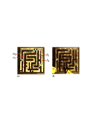
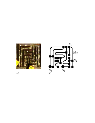
Figure 1: The experiment in [NYT00] (reprinted from there): (a) shows the maze uniformly covered by Physarum; yellow color indicates presence of Physarum. Food (oatmeal) is provided at the locations labeled AG. After a while the mold retracts to the shortest path connecting the food sources as shown in (b) and (c). (d) shows the underlying abstract graph. The video [Phy10] shows the experiment.

Physarum polycephalum is a slime mold that apparently is able to solve shortest path problems. Nakagaki, Yamada, and Tóth [NYT00] report about the following experiment; see Figure 1. They built a maze, covered it by pieces of Physarum (the slime can be cut into pieces which will reunite if brought into vicinity), and then fed the slime with oatmeal at two locations. After a few hours the slime retracted to a path that follows the shortest path in the maze connecting the food sources. The authors report that they repeated the experiment with different mazes; in all experiments, Physarum retracted to the shortest path.

The paper [TKN07] proposes a mathematical model for the behavior of the slime and argues extensively that the model is adequate. Physarum is modeled as an electrical network with time varying resistors. We have a simple undirected graph $G=(N,E)$ with distinguished nodes $s_{0}$ and $s_{1}$ modeling the food sources. Each edge $e\in E$ has a positive length $c_{e}$ and a positive capacity $x_{e}(t)$; $c_{e}$ is fixed, but $x_{e}(t)$ is a function of time. The resistance $r_{e}(t)$ of $e$ is $r_{e}(t)=c_{e}/x_{e}(t)$. In the electrical network defined by these resistances, a current of value 1 is forced from $s_{0}$ to $s_{1}$. For an (arbitrarily oriented) edge $e=(u,v)$, let $q_{e}(t)$ be the resulting current over $e$. Then, the capacity of $e$ evolves according to the differential equation

$$\dot{x}_{e}(t)=|q_{e}(t)|-x_{e}(t),$$ (1)

where $\dot{x}_{e}$ is the derivative of $x_{e}$ with respect to time. In equilibrium ($\dot{x}_{e}=0$ for all $e$), the flow through any edge is equal to its capacity. In non-equilibrium, the capacity grows (shrinks) if the absolute value of the flow is larger (smaller) than the capacity. In the sequel, we will mostly drop the argument $t$ as is customary in the treatment of dynamical systems. We will also write $q$ for the vector with components $q_{e}$. It is well-known that the electrical flow $q$ is the feasible flow minimizing energy dissipation $\sum_{e}r_{e}q_{e}^{2}$ (Thomson’s principle).

We refer to the dynamics above as biologically-grounded, as it was introduced by biologists to model the behavior of a biological system. Miyaji and Ohnishi were the first to analyze convergence for special graphs (parallel links and planar graphs with source and sink on the same face) in [MO08]. In [BMV12] convergence was proven for all graphs. We state the result from [BMV12] for the special case that the shortest path is unique.

Theorem 1.1 ([BMV12]).

Assume $x_{e}(0)>0$ and $c_{e}>0$ for all $e$, and that the undirected shortest path $P^{*}$ from $s_{0}$ to $s_{1}$ w.r.t. the cost vector $c$ is unique. Then $x(t)$ in (1) converges to $P^{*}$. Namely, $x_{e}(t)\rightarrow 1$ for $e\in P^{*}$ and $x_{e}\rightarrow 0$ for $e\not\in P^{*}$ as $t\rightarrow\infty$.

[BMV12] also proves an analogous result for the undirected transportation problem; [Bon13] simplified the argument under additional assumptions. The paper [Bon15] studies a more general dynamics and proves convergence for parallel links.

In this paper, we extend this result to non-negative undirected linear programs

$$\min\{c^{\mathrm{T}}x:Af=b,\ |f|\leq x\},$$ (2)

where $A\in\mathbb{R}^{n\times m}$, $b\in\mathbb{R}^{n}$, $x\in\mathbb{R}^{m}$, $c\in\mathbb{R}_{\geq 0}^{m}$, and the absolute values are taken componentwise. Undirected LPs can model a wide range of problems, e.g., optimization problems such as shortest path and min-cost flow in undirected graphs, and the Basis Pursuit problem in signal processing [CDS98].

We use $n$ for the number of rows of $A$ and $m$ for the number of columns, since this notation is appropriate when $A$ is the node-edge-incidence matrix of a graph. A vector $f\in\mathbb{R}^{m}$ is feasible if $Af=b$. We assume that the system $Af=b$ has a feasible solution and every nonzero vector $f$ in the kernel  of $A$ has positive cost $\sum_{e}c_{e}|f_{e}|>0$. The vector $q\in\mathbb{R}^{m}$ in (1) is now the minimum energy feasible solution

$$q(t)=\mathop{\rm argmin}_{f\in\mathbb{R}^{m}}\left\{\sum_{e:x_{e}\neq 0}\frac{c_{e}}{x_{e}(t)}f_{e}^{2}:Af=b\wedge f_{e}=0\text{ whenever }x_{e}=0\right\}.$$ (3)

We remark that $q$ is unique; see Subsection 3.1.1. If $A$ is the incidence matrix of a graph (the column corresponding to an edge $e$ has one entry $+1$, one entry $-1$ and all other entries are equal to zero), (2) is a transshipment problem with flow sources and sinks encoded by a demand vector $b$. The condition that there is no solution in the kernel of $A$ with $c_{e}f_{e}=0$ for all $e$ states that every cycle contains at least one edge of positive cost. In that setting, $q(t)$ as defined by (3) coincides with the electrical flow induced by resistors of value $c_{e}/x_{e}(t)$. We can now state our first main result.

Theorem 1.2.

Let $c\geq 0$ satisfy $c^{\mathrm{T}}|f|>0$ for every non-zero $f$ in the kernel of $A$. Let $x^{*}$ be an optimum solution of (2) and let $X_{\star}$ be the set of optimum solutions. Assume $x(0)>0$. The following holds for the dynamics (1) with $q$ as in (3):

1. The solution $x(t)$ exists for all $t\geq 0$.

2. The cost $c^{\mathrm{T}}x(t)$ converges to $c^{\mathrm{T}}x^{*}$ as $t$ goes to infinity.

3. The vector $x(t)$ converges to $X_{\star}$, i.e., $\lim_{t\rightarrow\infty}\inf\left\{\,|\!|x(t)-x^{\prime}|\!|\mbox{ {\rm:} }x^{\prime}\in X_{\star}\,\right\}\rightarrow 0$.

4. For all $e$ with $c_{e}>0$, $x_{e}(t)-|q_{e}(t)|$ converges to zero as $t$ goes to infinity.  If $x^{*}$ is unique, $x(t)$ and $q(t)$ converge to $x^{*}$ as $t$ goes to infinity.

Item (i) was previously shown in [SV16a] for the case of a strictly positive cost vector. The result in [SV16a] is actually stated only for the all-ones cost vector $c=\bf{1}$. The case of a general positive cost vector reduces to this special case by rescaling the solution vector $x$. Item $(i)$ for the more general cost vector and items $(ii)$ to $(iv)$ are new. We stress that the dynamics (1) is biologically-grounded. It was proposed to model a biological system and not as an optimization method. Nevertheless, it can solve a large class of non-negative LPs. Table 1 summarizes our first main result and puts it into context.

Reference	Problem (Undirected Case)	Existence of Solution	Convergence to $\mathrm{OPT}$	Comments
[MO08]	Shortest Path	Yes	Yes	parallel edges, planar graphs
[BMV12]	Shortest Path	Yes	Yes	all graphs
[SV16a]	Positive LP	Yes	No	$c>0$
Our Result	Nonnegative LP	Yes	Yes	1) $c\geq 0$ 2) $\forall v\in\mathrm{ker}(A)\,:\,c^{\mathrm{T}}|v|>0$

Table 1: Convergence results for the continuous undirected Physarum dynamics (1).

Sections 2 and 3 are devoted to the proof of our first main theorem. For ease of exposition, we present the proof in two steps. In Section 2, we give a proof under the following simplifying assumptions.

1. $c>0$,

2. The basic feasible solutions of (2) have distinct cost,

3. We start with a positive vector $x(0)\in X_{\mathrm{dom}}\mathbin{\raisebox{0.21529pt}{\mbox{\rm:}}\!\!=}\left\{\,x\in\mathbb{R}^{n}\mbox{ {\rm:} }\text{there is a feasible $f$ with $|f|\leq x$}\,\right\}$.

Section 2 generalizes [Bon13]. For the undirected shortest path problem, condition (B) states that all simple undirected source-sink paths have distinct cost and condition (C) states that all source-sink cuts have a capacity of at least one at time zero (and hence at all times). The existence of a solution with domain $[0,\infty)$ was already shown in [SV16a]. We will show that $X_{\mathrm{dom}}$ is an invariant set, i.e., the solution stays in $X_{\mathrm{dom}}$ for all times, and that $E(x)=\sum_{e}r_{e}x_{e}^{2}=\sum_{e}c_{e}x_{e}$ is a Lyapunov function  [LaS76, Tes12] for the dynamics (1), i.e., $\dot{E}\leq 0$ and $\dot{E}=0$ if and only if $\dot{x}=0$. It follows from general theorems about dynamical systems that the dynamics converges to a fixed point of (1). The fixed points are precisely the vectors $|f|$ where $f$ is a feasible solution of (2). A final argument establishes that the dynamics converges to a fixed point of minimum cost.

In Section 3, we prove the general case of the first main theorem. We assume

1. $c\geq 0$,

2. ${\mathrm{cost}}(z)=c^{\mathrm{T}}|z|>0$ for every non-zero vector $z$ in the kernel of $A$,

3. We start with a positive vector $x(0)>0$.

Section 3 generalizes [BMV12] in two directions. First, we treat general undirected LPs and not just the undirected shortest path problem, respectively, the transshipment problem. Second, we replace the condition $c>0$ by the requirement $c\geq 0$ and every non-zero vector in the kernel of $A$ has positive cost. For the undirected shortest path problem, the latter condition states that the underlying undirected graph has no zero-cost cycle. Section 3 is technically considerably more difficult than Section 2. We first establish the existence of a solution with domain $[0,\infty)$. To this end, we derive a closed formula for the minimum energy feasible solution and prove that the mapping $x\mapsto q$ is locally Lipschitz. Existence of a solution with domain $[0,\infty)$ follows by standard arguments. We then show that $X_{\mathrm{dom}}$ is an attractor, i.e., the solution $x(t)$ converges to $X_{\mathrm{dom}}$. We next characterize equilibrium points and exhibit a Lyapunov function. The Lyapunov function is a normalized version of $E(x)$. The normalization factor is equal to the optimal value of the linear program $\max\left\{\,\alpha\mbox{ {\rm:} }Af=\alpha b,\ |f|\leq x\,\right\}$ in the variables $f$ and $\alpha$. Convergence to an equilibrium point follows from the existence of a Lyapunov function. A final argument establishes that the dynamics converges to a fixed point of minimum cost.

1.2 The Biologically-Inspired Model

Ito et al. [IJNT11] initiated the study of the dynamics

$$\dot{x}(t)=q(t)-x(t).$$ (4)

We refer to this dynamics as the directed dynamics in contrast to the undirected dynamics (1). The directed dynamics is biologically-inspired – the similarity to (1) is the inspiration. It was never claimed to model the behavior of a biological system. Rather, it was introduced as a biologically-inspired optimization method. The work in [IJNT11] shows convergence of this directed dynamics (4) for the directed shortest path problem and [JZ12, SV16c, Bon16] show convergence for general positive linear programs, i.e., linear programs with positive cost vector $c>0$ of the form

$$\min\{c^{\mathrm{T}}x:Ax=b,\ x\geq 0\}.$$ (5)

The discrete versions of both dynamics define sequences $x^{(t)}$, $t=0,1,2,\ldots$ through

$$x^{(t+1)} =(1-h^{(t)})x^{(t)}+h^{(t)}q^{(t)} \text{discrete directed dynamics};$$ (6)

$$x^{(t+1)} =(1-h^{(t)})x^{(t)}+h^{(t)}|q^{(t)}| \text{discrete undirected dynamics},$$ (7)

where $h^{(t)}$ is the step size and $q^{(t)}$ is the minimum energy feasible solution as in (3). For the discrete dynamics, we can ask complexity questions. This is particularly relevant for the discrete directed dynamics as it was designed as an biologically-inspired optimization method.

For completeness, we review the state-of-the-art results for the discrete undirected dynamics. For the undirected shortest path problem, the convergence of the discrete undirected dynamics (7) was shown in [BBD⁺13]. The convergence proof gives an upper bound on the step size and on the number of steps required until an $\varepsilon$-approximation of the optimum is obtained. [SV16b] extends the result to the transshipment problem and [SV16a] further generalizes the result to the case of positive LPs. The paper [SV16b] is related to our first result. It shows convergence of the discretized undirected dynamics (7), we show convergence of the continuous undirected dynamics (1) for a more general cost vector.

We come to the discrete directed Physarum-inspired dynamics (6). Similarly to the undirected setting, Becchetti et al. [BBD⁺13] showed the convergence of (6) for the shortest path problem. Straszak and Vishnoi extended the analysis to the transshipment problem [SV16b] and positive LPs [SV16c].

Theorem 1.3.

[SV16c, Theorem 1.3] Let $A\in\mathbb{Z}^{n\times m}$ have full row rank $(n\leq m)$, $b\in\mathbb{Z}^{n}$, $c\in\mathbb{Z}_{>0}^{m}$, and let $D_{S}:=\max\{|\det(M)|\,:\,M\text{ is a square sub-matrix of }A\}$. Suppose the Physarum-inspired dynamics (6) is initialized with a feasible point $x^{(0)}$ of (5) such that $M^{-1}\leq x^{(0)}\leq M$ and $c^{\mathrm{T}}x^{(0)}\leq M\cdot{\mathrm{opt}}$ for some $M\geq 1$, where ${\mathrm{opt}}$ denotes the optimum cost of (5). Then, for any $\varepsilon>0$ and step size $h\leq\varepsilon/(\sqrt{6}{|\!|c|\!|_{1}}D_{S})^{2}$, after $k=O((\varepsilon h)^{-2}\ln M)$ steps, $x^{(k)}$ is a feasible solution with $c^{\mathrm{T}}x^{(k)}\leq(1+\varepsilon){\mathrm{opt}}$.

Theorem 1.3 gives an algorithm that computes a $(1+\varepsilon)$-approximation to the optimal cost of (5). In comparison to [BBD⁺13, SV16b], it has several shortcomings. First, it requires a feasible starting point. Second, the step size depends linearly on $\varepsilon$. Third, the number of steps required to reach an $\varepsilon$-approximation has a quartic dependence on ${\mathrm{opt}}/(\varepsilon\Phi)$. In contrast, the analysis in [BBD⁺13, SV16b] yields a step size independent of $\varepsilon$ and a number of steps that depends only logarithmically on $1/\varepsilon$, see Table 2.

We overcome these shortcomings. Before we can state our result, we need some notation. Let $X_{\star}$ be the set of optimal solutions to (5). The distance of a capacity vector $x$ to $X_{\star}$ is defined as

$$\mathrm{dist}(x,X_{\star}):=\inf\{|\!|x-x^{\prime}|\!|_{\infty}\,:\,x^{\prime}\in X_{\star}\}.$$

Let $\gamma_{A}:=\gcd(\{A_{ij}:A_{ij}\neq 0\})\in\mathbb{Z}_{>0}$ and

$$D:=\max\left\{\left|\det\left(M\right)\right|\,:\,M\text{ is a square submatrix of }A/\gamma_{A}\text{ with dimension }n-1\text{ or }n\right\}.$$ (8)

Let $\mathcal{N}$ be the set of non-optimal basic feasible solution of (5) and

$$\Phi:=\min_{g\in\mathcal{N}}c^{\mathrm{T}}g-{\mathrm{opt}}\geq 1/(D\gamma_{A})^{2},$$ (9)

where the inequality is well known [PS82, Lemma 8.6]. For completeness, we present a proof in Subsection 4.5. Informally, our second main result proves the following properties of the Physarum-inspired dynamics (6):

1. For any $\varepsilon>0$ and any strongly dominating starting point $x^{(0)}$, there is a fixed step size $h(x^{(0)})$ such that the Physarum-inspired dynamics (6) initialized with $x^{(0)}$ and $h(x^{(0)})$ converges to $X_{\star}$, i.e., $\mathrm{dist}(x^{(k)},X_{\star})<\varepsilon/(D\gamma_{A})$ for large enough $k$.

2. The step size can be chosen independently of $\varepsilon$.

3. The number of steps $k$ depends logarithmically on $1/\varepsilon$ and quadratically on ${\mathrm{opt}}/\Phi$.

4. The efficiency bounds depend on a scale-invariant determinant $D$.

In Section 4.8, we establish a corresponding lower bound. We show that for the Physarum-inspired dynamics (6) to compute a point $x^{(k)}$ such that $\mathrm{dist}(x^{(k)},X_{\star})<\varepsilon$, the number of steps required for computing an $\varepsilon$-approximation has to grow linearly in ${\mathrm{opt}}/(h\Phi)$ and $\ln(1/\varepsilon)$, i.e. $k\geq\Omega({\mathrm{opt}}\cdot(h\Phi)^{-1}\cdot\ln(1/\varepsilon))$. Table 2 puts our results into context.

We state now our second main result for the special case of a feasible starting point, and we provide the full version in Theorem 4.2 which applies for arbitrary strongly dominating starting point, see Section 4. We use the following constants in the statement of the bounds.

1. $h_{0}:=c_{\min}/(4D{|\!|c|\!|_{1}})$, where $c_{\min}:=\min_{i}\{c_{i}\}$;

2. $\Psi^{(0)}:=\max\{mD^{2}\|b/\gamma_{A}\|_{1},\|x^{(0)}\|_{\infty}\}$;

3. $C_{1}:=D\|b/\gamma_{A}\|_{1}{|\!|c|\!|_{1}}$, $\,C_{2}:=8^{2}m^{2}nD^{5}\gamma_{A}^{2}|\!|A|\!|_{\infty}\lVert b\rVert_{1}\,$ and $\,C_{3}:=D^{3}\gamma_{A}{|\!|b|\!|_{1}}{|\!|c|\!|_{1}}$.

Theorem 1.4.

Suppose $A\in\mathbb{Z}^{n\times m}$ has full row rank $(n\leq m)$, $b\in\mathbb{Z}^{n}$, $c\in\mathbb{Z}_{>0}^{m}$ and $\varepsilon\in(0,1)$. Given a feasible starting point $x^{(0)}>0$ the Physarum-inspired dynamics (6) with step size $h\leq(\Phi/{\mathrm{opt}})\cdot h_{0}^{2}/2$ outputs for any $k\geq 4C_{1}/(h\Phi)\cdot\ln(C_{2}\Psi^{(0)}/(\varepsilon\cdot\min\{1,x_{\min}^{(0)}\}))$ a feasible $x^{(k)}>0$ such that $\mathrm{dist}(x^{(k)},X_{\star})<\varepsilon/(D\gamma_{A})$.

Reference	Problem (Directed Case)	step size $h$	number of steps $k$	Guarantee
[BBD+13]	Shortest Path	indep. of $\varepsilon$	$\mathrm{poly}(m,n,{|\!|c|\!|_{1}},{|\!|x^{(0)}|\!|_{1}})$ $\cdot\ln(1/\varepsilon)$	$\mathrm{dist}(x^{(k)},X_{\star})<\varepsilon$
[SV16b]	Transshipment	indep. of $\varepsilon$	$\mathrm{poly}(m,n,{|\!|c|\!|_{1}},{|\!|b|\!|_{1}},{|\!|x^{(0)}|\!|_{1}})$ $\cdot\ln(1/\varepsilon)$	$\mathrm{dist}(x^{(k)},X_{\star})<\varepsilon$
[SV16c]	Positive LP	depends on $\varepsilon$	$\mathrm{poly}({|\!|c|\!|_{1}},D_{S},\ln{|\!|x^{(0)}|\!|_{1}})$ $\cdot$ $1/(\Phi\varepsilon)^{4}$	$c^{\mathrm{T}}x^{(k)}\leq(1+\varepsilon){\mathrm{opt}}$ $c^{\mathrm{T}}x^{(k)}<\min_{g\in\mathcal{N}}c^{\mathrm{T}}g$
Our Result	Positive LP	indep. of $\varepsilon$	$\mathrm{poly}({|\!|c|\!|_{1}},{|\!|b|\!|_{1}},D,\gamma_{A},\ln{|\!|x^{(0)}|\!|_{1}})$ $\cdot\Phi^{-2}\ln(1/\varepsilon)$	$\mathrm{dist}(x^{(k)},X_{\star})<\frac{\varepsilon}{D\gamma_{A}}$
Lower Bound	Positive LP	indep. of $\varepsilon$	$\Omega({\mathrm{opt}}\cdot(h\Phi)^{-1}\ln(1/\varepsilon))$	$\mathrm{dist}(x^{(k)},X_{\star})<\varepsilon$

Table 2: Convergence results for the discrete directed Physarum-inspired dynamics (6).

We stated the bounds on $h$ in terms of the unknown quantities $\Phi$ and ${\mathrm{opt}}$. However, $\Phi/{\mathrm{opt}}\geq 1/C_{3}$ by Lemma 3.1 and hence replacing $\Phi/{\mathrm{opt}}$ by $1/C_{3}$ yields constructive bounds for $h$. Note that the upper bound on the step size does not depend on $\varepsilon$ and that the bound on the number of iterations depends logarithmically on $1/\varepsilon$ and quadratically on ${\mathrm{opt}}/\Phi$.

What can be done if the initial point is not strongly dominating? For the transshipment problem it suffices to add an edge of high capacity and high cost from every source node to every sink node [BBD⁺13, SV16b]. This will make the instance strongly dominating and will not affect the optimal solution. We generalize this observation to positive linear programs. We add an additional column equal to $b$ and give it sufficiently high capacity and cost. This guarantees that the resulting instance is strongly dominating and the optimal solution remains unaffected. Moreover, our approach generalizes and improves upon [SV16b, Theorem 1.2], see Section 4.7.

Proof Techniques:

The crux of the analysis in [IJNT11, BBD⁺13, SV16b] is to show that for large enough $k$, $x^{(k)}$ is close to a non-negative flow $f^{(k)}$ and then to argue that $f^{(k)}$ is close to an optimal flow $f^{\star}$. This line of arguments yields a convergence of $x^{(k)}$ to $X_{\star}$ with a step size $h$ chosen independently of $\varepsilon$.

In Section 4, we extend the preceding approach to positive linear programs, by generalizing the concept of non-negative cycle-free flows to non-negative feasible kernel-free vectors (Subsection 4.4). Although, we use the same high level ideas as in [BBD⁺13, SV16b], we stress that our analysis generalizes all relevant lemmas in [BBD⁺13, SV16b] and it uses arguments from linear algebra and linear programming duality, instead of combinatorial arguments. Further, our core efficiency bounds (Subsection 4.2) extend [SV16c] and yield a scale-invariant determinant dependence of the step size and are applicable for any strongly dominating point (Subsection 4.3).

2 Convergence of the Physarum Dynamics: Simple Instances

In this section, we prove Theorem 1.2 under the simplifying assumptions (A) to (C), defined in page A.

2.1 Preliminaries

Note that we may assume that $A$ has full row-rank since any equation that is linearly dependent on other equations can be deleted without changing the feasible set. We continue to use $n$ and $m$ for the dimension of $A$. Thus, $A$ has rank $n$. We continue by fixing some terms and notation. A basic feasible solution of (2) is a pair of vectors $x$ and $f=(f_{B},f_{N})$, where $f_{B}=A_{B}^{-1}b$ and $A_{B}$ is a square $n\times n$ non-singular sub-matrix of $A$ and $f_{N}=0$ is the vector indexed by the coordinates not in $B$, and $x=|f|$. Since $f$ uniquely determines $x$, we may drop the latter for the sake of brevity and call $f$ a basic feasible solution of (2). A feasible solution $f$ is kernel-free or non-circulatory if it is contained in the convex hull of the basic feasible solutions. We say that a vector $f^{\prime}$ is sign-compatible with a vector $f$ (of the same dimension) or $f$-sign-compatible if $f^{\prime}_{e}\not=0$ implies $f^{\prime}_{e}f_{e}>0$. In particular, $\operatorname{{\mathrm{supp}}}(f^{\prime})\subseteq\operatorname{{\mathrm{supp}}}(f)$. For a given capacity vector $x$ and a vector $f\in\mathbb{R}^{m}$ with $\operatorname{{\mathrm{supp}}}(f)\subseteq\operatorname{{\mathrm{supp}}}(x)$, we use $E(f)=\sum_{e}(c_{e}/x_{e})f_{e}^{2}$ to denote the energy of $f$. The energy of $f$ is infinite, if $\operatorname{{\mathrm{supp}}}(f)\not\subseteq\operatorname{{\mathrm{supp}}}(x)$. We use ${\mathrm{cost}}(f)=\sum_{e}c_{e}|f_{e}|=c^{\mathrm{T}}|f|$ to denote the cost of $f$. Note that $E(x)=\sum_{e}(c_{e}/x_{e})x_{e}^{2}=\sum_{e}c_{e}x_{e}={\mathrm{cost}}(x)$. We define the constants $c_{\max}=\|c\|_{\infty}$ and $c_{\min}=\min_{e:c_{e}>0}c_{e}$.

We use the following corollary of the finite basis theorem for polyhedra.

Lemma 2.1.

Let $f$ be a feasible solution of (2). Then $f$ is the sum of a convex combination of at most $m$ basic feasible solutions plus a vector in the kernel of $A$. Moreover, all elements in this representation are sign-compatible with $f$.

Proof.

We may assume $f\geq 0$. Otherwise, we flip the sign of the appropriate columns of $A$. Thus, the system $Af=b,\ f\geq 0$ is feasible and $f$ is the sum of a convex combination of at most $m$ basic feasible solutions plus a vector in the kernel of $A$ by the finite basis theorem [Sch99, Corollary 7.1b]. By definition, the elements in this representation are non-negative vectors and hence sign-compatible with $f$. ∎

Lemma 2.2 (Grönwall’s Lemma).

Let $A,B,\alpha,\beta\in\mathbb{R}$, $\alpha\not=0$, $\beta\not=0$, and let $g$ be a continuous differentiable function on $[0,\infty)$. If $A+\alpha g(t)\leq\dot{g}(t)\leq B+\beta g(t)$ for all $t\geq 0$, then $-A/\alpha+(g(0)+A/\alpha)e^{\alpha t}\leq g(t)\leq-B/\beta+(g(0)+B/\beta)e^{\beta t}$ for all $t\geq 0$.

Proof.

We show the upper bound. Assume first that $B=0$. Then

$$\frac{d}{dt}\frac{g}{e^{\beta t}}=\frac{\dot{g}e^{\beta t}-\beta ge^{\beta t}}{e^{2\beta t}}\leq 0\quad\text{implies}\quad\frac{g(t)}{e^{\beta t}}\leq\frac{g(0)}{e^{\beta 0}}=g(0).$$

If $B\not=0$, define $h(t)=g(t)+B/\beta$. Then

$$\dot{h}=\dot{g}\leq B+\beta g=B+\beta(h-B/\beta)=\beta h$$

and hence $h(t)\leq h(0)e^{\beta t}$. Therefore $g(t)\leq-B/\beta+(g(0)+B/\beta)e^{\beta t}$. ∎

An immediate consequence of Grönwall’s Lemma is that the undirected Physarum dynamics (1) initialized with any positive starting vector $x(0)$, generates a trajectory $\{x(t)\}_{t\geq 0}$ such that each time state $x(t)$ is a positive vector. Indeed, since $\dot{x}_{e}=|q_{e}|-x_{e}\geq-x_{e}$, we have $x_{e}(t)\geq x_{e}(0)\cdot\exp\{-t\}$ for every index $e$ with $x_{e}(0)>0$ and every time $t$. Further, by (1) and (3), it holds for indices $e$ with $x_{e}(0)=0$ that $x_{e}(t)=0$ for every time $t$. Hence, the trajectory $\{x(t)\}_{t\geq 0}$ has a time-invariant support.

Lemma 2.3 ([JZ12]).

Let $R=\mathrm{diag}(c_{e}/x_{e})$. Then $q=R^{-1}A^{\mathrm{T}}p$, where $p=(AR^{-1}A^{\mathrm{T}})^{-1}b$.

Proof.

$q$ minimizes $\sum_{e}r_{e}q_{e}^{2}$ subject to $Aq=b$. The Karush-Kuhn-Tucker (KKT) optimality conditions for constrained optimization [Boy04] imply the existence of a vector $p$ such that $Rq=A^{\mathrm{T}}p$. Substituting into $Aq=b$ yields $p=(AR^{-1}A^{\mathrm{T}})^{-1}b$. ∎

Lemma 2.4.

$X_{\mathrm{dom}}$ is an invariant set, i.e., if $x(0)\in X_{\mathrm{dom}}$ then $x(t)\in X_{\mathrm{dom}}$ for all $t$.

Proof.

Let $q(t)$ be the minimum energy feasible solution with respect to $R(t)=\mathrm{diag}(c_{e}/x_{e}(t))$, and let $f(t)$ be such that $f(0)$ is feasible, $|f(0)|\leq x(0)$, and $\dot{f}(t)=q(t)-f(t)$. Then $\frac{d}{dt}(Af-b)=A(q-f)=b-Af$ and hence $Af(t)-b=(Af(0)-b)e^{-t}=0$. Thus $f(t)$ is feasible for all $t$. Moreover,

$$\frac{d}{dt}(f-x)=\dot{f}-\dot{x}=q-f-(|q|-x)=q-|q|-(f-x)\leq-(f-x).$$

Thus $f(t)-x(t)\leq(f(0)-x(0))e^{-t}\leq 0$ by Grönwall’s Lemma applied with $g(t)=f(t)-x(t)$ and $\beta=-1$, and hence $f(t)\leq x(t)$ for all $t$. Similarly,

$$\frac{d}{dt}(f+x)=\dot{f}+\dot{x}=q-f+(|q|-x)=q+|q|-(f+x)\geq-(f+x).$$

Thus $f(t)+x(t)\geq(f(0)+x(0))e^{-t}\geq 0$ by Grönwall’s Lemma applied with $g(t)=f(t)+x(t)$ and $\alpha=-1$ and $A=0$, and hence $f(t)\geq-x(t)$ for all $t$.

We conclude that $|f(t)|\leq x(t)$ for all $t$. Thus, $x(t)\in X_{\mathrm{dom}}$ for all $t$. ∎

2.2 The Convergence Proof

We will first characterize the equilibrium points. They are precisely the points $|f|$, where $f$ is a basic feasible solution; the proof uses assumption (B) in page A. We then show that $E(x)$ is a Lyapunov function for (1), in particular, $\dot{E}\leq 0$ and $\dot{E}=0$ if and only if $x$ is an equilibrium point. For this argument, we need that the energy of $q$ is at most the energy of $x$ with equality if and only if $x$ is an equilibrium point. This proof uses assumptions (A) and (C) in page A. It follows from the general theory of dynamical systems that $x(t)$ approaches an equilibrium point. Finally, we show that convergence to a non-optimal equilibrium is impossible.

Lemma 2.5 (Generalization of Lemma 2.3 in [Bon13]).

Assume (A) to (C). If $f$ is a basic feasible solution of (2), then $x=|f|$ is an equilibrium point. Conversely, if $x$ is an equilibrium point, then $x=|f|$ for some basic feasible solution $f$.

Proof.

Let $f$ be a basic feasible solution, let $x=|f|$, and let $q$ be the minimum energy feasible solution with respect to the resistances $c_{e}/x_{e}$. We have $Aq=b$ and $\operatorname{{\mathrm{supp}}}(q)\subseteq\operatorname{{\mathrm{supp}}}(x)$ by definition of $q$. Since $f$ is a basic feasible solution there is a subset $B$ of size $n$ of the columns of $A$ such that $A_{B}$ is non-singular and $f=(A_{B}^{-1}b,0)$. Since $\operatorname{{\mathrm{supp}}}(q)\subseteq\operatorname{{\mathrm{supp}}}(x)\subseteq B$, we have $q=(q_{B},0)$ for some vector $q_{B}$. Thus, $b=Aq=A_{B}q_{B}$ and hence $q_{B}=f_{B}$. Therefore $\dot{x}=|q|-x=0$ and $x$ is an equilibrium point.

Conversely, if $x$ is an equilibrium point, $|q_{e}|=x_{e}$ for every $e$. By changing the signs of some columns of $A$, we may assume $q\geq 0$. Then $q=x$. Since $q_{e}=x_{e}/c_{e}A_{e}^{\mathrm{T}}p$ where $A_{e}$ is the $e$-th column of $A$ by Lemma 2.3, we have $c_{e}=A_{e}^{\mathrm{T}}p$, whenever $x_{e}>0$. By Lemma 2.1, $q$ is a convex combination of basic feasible solutions and a vector in the kernel of $A$ that are sign-compatible with $q$. The vector in the kernel must be zero as $q$ is a minimum energy feasible solution. For any basic feasible solution $z$ contributing to $q$, we have $\operatorname{{\mathrm{supp}}}(z)\subseteq\operatorname{{\mathrm{supp}}}(x)$. Summing over the $e\in\operatorname{{\mathrm{supp}}}(z)$, we obtain ${\mathrm{cost}}(z)=\sum_{e\in\operatorname{{\mathrm{supp}}}(z)}c_{e}z_{e}=\sum_{e\in\operatorname{{\mathrm{supp}}}(z)}z_{e}A_{e}^{\mathrm{T}}p=b^{\mathrm{T}}p$. Thus, the convex combination involves only a single basic feasible solution by assumption (B) and hence $x$ is a basic feasible solution. ∎

The vector $x(t)$ dominates a feasible solution at all times. Since $q(t)$ is the minimum energy feasible solution at time $t$, this implies $E(q(t))\leq E(x(t))$ at all times. A further argument shows that we have equality if and only if $x=|q|$.

Lemma 2.6 (Generalization of Lemma 3.1 in  [Bon13]).

Assume (A) to (C). At all times, $E(q)\leq E(x)$. If $E(q)=E(x)$, then $x=|q|$.

Proof.

Recall that $x(t)\in X_{\mathrm{dom}}$ for all $t$. Thus, at all times, there is a feasible $f$ such that $|f|\leq x$. Since $q$ is a minimum energy feasible solution, we have

$$E(q)\leq E(f)\leq E(x).$$

If $E(q)=E(x)$ then $E(q)=E(f)$ and hence $q=f$ since the minimum energy feasible solution is unique. Also, $|f|=x$ since $|f|\leq x$ and $|f_{e}|<x_{e}$ for some $e$ implies $E(f)<E(x)$. The last conclusion uses $c>0$. ∎

Lyapunov functions are the main tool for proving convergence of dynamical systems. We show that $E(x)$ is a Lyapunov function for (1).

Lemma 2.7 (Generalization of Lemma 3.2 in [Bon13]).

Assume (A) to (C). $E(x)$ is a Lyapunov function for (1), i.e., it is continuous as a function of $x$, $E(x)\geq 0$, $\dot{E}(x)\leq 0$ and $\dot{E}(x)=0$ if and only if $\dot{x}=0$.

Proof.

$E$ is clearly continuous and non-negative. Recall that $E(x)={\mathrm{cost}}(x)$. Let $R$ be the diagonal matrix with entries $c_{e}/x_{e}$. Then

$$\frac{d}{dt}{{\mathrm{cost}}(x)} =c^{\mathrm{T}}(|q|-x)$$ by (1)

$$=x^{\mathrm{T}}R|q|-x^{\mathrm{T}}Rx c=Rx$$ since

$$=x^{\mathrm{T}}R^{1/2}R^{1/2}|q|-x^{\mathrm{T}}Rx$$

$$\leq(q^{\mathrm{T}}Rq)^{1/2}(x^{\mathrm{T}}Rx)^{1/2}-x^{\mathrm{T}}Rx$$ by Cauchy-Schwarz

$$\leq(x^{\mathrm{T}}Rx)^{1/2}(x^{\mathrm{T}}Rx)^{1/2}-x^{\mathrm{T}}Rx$$ by Lemma 2.6

$$=0.$$

Observe that $\frac{d}{dt}{{\mathrm{cost}}(x)}=0$ implies that both inequalities above are equalities. This is only possible if the vectors $|q|$ and $x$ are parallel and $E(q)=E(x)$. Thus, $x=|q|$ by Lemma 2.6. ∎

It follows now from the general theory of dynamical systems that $x(t)$ converges to an equilibrium point.

Corollary 2.8 (Generalization of Corollary 3.3. in [Bon13].).

Assume (A) to (C). As $t\rightarrow\infty$, $x(t)$ approaches an equilibrium point and $c^{\mathrm{T}}x(t)$ approaches the cost of the corresponding basic feasible solution.

Proof.

The proof in [Bon13] carries over. We include it for completeness. The existence of a Lyapunov function $E$ implies by [LaS76, Corollary 2.6.5] that $x(t)$ approaches the set $\left\{\,x\in\mathbb{R}_{\geq 0}^{m}\mbox{ {\rm:} }\dot{E}=0\,\right\}$, which by Lemma 2.7 is the same as the set $\left\{\,x\in\mathbb{R}_{\geq 0}^{m}\mbox{ {\rm:} }\dot{x}=0\,\right\}$. Since this set consists of isolated points (Lemma 2.5), $x(t)$ must approach one of those points, say the point $x_{0}$. When $x=x_{0}$ , one has $E(q)=E(x)={\mathrm{cost}}(x)=c^{\mathrm{T}}x$. ∎

It remains to exclude that $x(t)$ converges to a nonoptimal equilibrium point.

Theorem 2.9 (Generalization of Theorem 3.4 in [Bon13]).

Assume (A) to (C). As $t\rightarrow\infty$, $c^{\mathrm{T}}x(t)$ converges to the cost of the optimal solution and $x(t)$ converges to the optimal solution.

Proof.

By the corollary, it suffices to prove the second part of the claim. For the second part, assume that $x(t)$ converges to a non-optimal solution $z$. Let $x^{*}$ be the optimal solution and let $W=\sum_{e}x^{*}_{e}c_{e}\ln x_{e}$. Let $\delta=({\mathrm{cost}}(z)-{\mathrm{cost}}(x^{*}))/2$. Note that for all sufficiently large $t$, we have $E(q(t))\geq{\mathrm{cost}}(z)-\delta\geq{\mathrm{cost}}(x^{*})+\delta$. Further, by definition $q_{e}=(x_{e}/c_{e})A_{e}^{\mathrm{T}}p$ and thus

$$\dot{W}=\sum_{e}x^{*}_{e}c_{e}\frac{|q_{e}|-x_{e}}{x_{e}}=\sum_{e}x^{*}_{e}|A_{e}^{\mathrm{T}}p|-{\mathrm{cost}}(x^{*})\geq\sum_{e}x^{*}_{e}A_{e}^{\mathrm{T}}p-{\mathrm{cost}}(x^{*})\geq\delta,$$

where the last inequality follows by $\sum_{e}x^{*}_{e}A_{e}^{\mathrm{T}}p=b^{\mathrm{T}}p=E(q)\geq{\mathrm{cost}}(x^{*})+\delta$. Hence $W\rightarrow\infty$, a contradiction to the fact that $x$ is bounded. ∎

3 Convergence of the Physarum Dynamics: General Instances

In this section, we prove Theorem 1.2 under the more general assumptions (D) to (F), defined in page D.

3.1 Existence of a Solution with Domain $[0,\infty)$

In this subsection we show that a solution $x(t)$ to (1) has domain $[0,\infty)$. We first derive an explicit formula for the minimum energy feasible solution $q$ and then show that the mapping $x\mapsto q$ is Lipschitz continuous; this implies existence of a solution with domain $[0,\infty)$ by standard arguments.

3.1.1 The Minimum Energy Solution

Recall that for $\gamma_{A}=\gcd(\{A_{ij}:A_{ij}\neq 0\})\in\mathbb{Z}_{>0}$, we defined by

$$D=\max\left\{\left|\det\left(M\right)\right|\,:\,M\text{ is a square submatrix of }A/\gamma_{A}\text{ with dimension }n-1\text{ or }n\right\}.$$

We derive now properties of the minimum energy solution. In particular, if every non-zero vector in the kernel of $A$ has positive cost,

1. the minimum energy feasible solution is kernel-free and unique (Lemma 3.2),

2. $|q_{e}|\leq D{|\!|b/\gamma_{A}|\!|_{1}}$ for every $e\in[m]$ (Lemma 3.3),

3. $q$ is defined by (12) (Lemma 3.4), and

4. $E(q)=b^{\mathrm{T}}p$, where $p$ is defined by (12) (Lemma 3.5).

We note that for positive cost vector $c>0$, these results are known.

We proceed by establishing some useful properties on basic feasible solutions.

Lemma 3.1.

Suppose $A\in\mathbb{Z}^{n\times m}$ is an integral matrix, and $b\in\mathbb{Z}^{n}$ is an integral vector. Then, for any basic feasible solutions $f$ with $Af=b$ and $f\geq 0$, it holds that $|\!|f|\!|_{\infty}\leq D{|\!|b/\gamma_{A}|\!|_{1}}$ and $f_{j}\neq 0$ implies $|f_{j}|\geq 1/(D\gamma_{A})$.

Proof.

Since $f$ is a basic feasible solution, it has the form $f=\left(f_{B},0\right)$ such that $A_{B}\cdot f_{B}=b$ where $A_{B}\in\mathbb{Z}^{n\times n}$ is an invertible submatrix of $A$. We write $M_{-i,-j}$ to denote the matrix $M$ with deleted $i$-th row and $j$-th column. Let $Q_{j}$ be the matrix formed by replacing the $j$-th column of $A_{B}$ by the column vector $b$. Then, using the fact that $\det(tA)=t^{n}\det(A)$ for every $A\in\mathbb{R}^{n\times n}$ and $t\in\mathbb{Z}$, Cramer’s rule yields

$$\left|f_{B}(j)\right|=\left|\frac{\det\left(Q_{j}\right)}{\det\left(A_{B}\right)}\right|=\frac{1}{\gamma_{A}}\left|\sum_{k=1}^{n}\frac{\left(-1\right)^{j+k}\cdot b_{k}\cdot\det\left(\gamma_{A}^{-1}[A_{B}]_{-k,-j}\right)}{\det\left(\gamma_{A}^{-1}A_{B}\right)}\right|$$

By the choice of $\gamma_{A}$, the values $\det(\gamma_{A}^{-1}A_{B})$ and $\det(\gamma_{A}^{-1}[A_{B}]_{-k,-j})$ are integral for all $k$, it follows that

$$\left|f_{B}(j)\right|\leq D{|\!|b/\gamma_{A}|\!|_{1}}\qquad\text{and}\qquad f_{B}(j)\neq 0\quad\Longrightarrow\quad\frac{1}{D\gamma_{A}}\leq\left|f_{B}(j)\right|.\hfill\qed$$

Lemma 3.2.

If every non-zero vector in the kernel of $A$ has positive cost, the minimum energy feasible solution is kernel-free and unique.

Proof.

Let $q$ be a minimum energy feasible solution. Since $q$ is feasible, it can be written as $q_{n}+q_{r}$, where $q_{n}$ is a convex combination of basic feasible solutions and $q_{r}$ lies in the kernel of $A$. Moreover, all elements in this representation are sign-compatible with $q$ by Lemma 2.1. If $q_{r}\not=0$, the vector $q-q_{r}$ is feasible and has smaller energy, a contradiction. Thus $q_{r}=0$.

We next prove uniqueness. Assume for the sake of a contradiction that there are two distinct minimum energy feasible solutions $q^{(1)}$ and $q^{(2)}$. We show that the solution $(q^{(1)}+q^{(2)})/2$ uses less energy than $q^{(1)}$ and $q^{(2)}$. Since $h\mapsto h^{2}$ is a strictly convex function from $\mathbb{R}$ to $\mathbb{R}$, the average of the two solutions will be better than either solution if there is an index $e$ with $r_{e}>0$ and $q^{(1)}_{e}\not=q^{(2)}_{e}$. The difference $z=q^{(1)}-q^{(2)}$ lies in the kernel of $A$ and hence ${\mathrm{cost}}(z)=\sum_{e}c_{e}|z_{e}|>0$. Thus there is an $e$ with $c_{e}>0$ and $z_{e}\not=0$. We have now shown uniqueness. ∎

Lemma 3.3.

Assume that every non-zero vector in the kernel of $A$ has positive cost. Let $q$ be the minimum energy feasible solution. Then $|q_{e}|\leq D{|\!|b/\gamma_{A}|\!|_{1}}$ for every $e$.

Proof.

Since $q$ is a convex combination of basic feasible solutions, $|q_{e}|\leq\max_{z}|z_{e}|$ where $z$ ranges over basic feasible solutions of the form $(z_{B},0)$, where $z_{B}=A_{B}^{-1}b$ and $A_{B}\in\mathbb{R}^{n\times n}$ is a non-singular submatrix of $A$. Thus, by Lemma 3.1 every component of $z$ is bounded by $D{|\!|b/\gamma_{A}|\!|_{1}}$. ∎

In [SV16c], the bound $|q_{e}|\leq D^{2}m{|\!|b|\!|_{1}}$ was shown. We will now derive explicit formulae for the minimum energy solution $q$. We will express $q$ in terms of a vector $p\in\mathbb{R}^{n}$, which we refer to as the potential, by analogy with the network setting, in which $p$ can be interpreted as the electric potential of the nodes. The energy of the minimum energy solution is equal to $b^{\mathrm{T}}p$. We show that the mapping $x\mapsto q$ is locally Lipschitz. Note that for $c>0$ these facts are well-known. Let us split the column indices $[m]$ of $A$ into

$$P:=\left\{\,e\in[m]\mbox{ {\rm:} }c_{e}>0\,\right\}\quad\text{ and }\quad Z:=\left\{\,e\in[m]\mbox{ {\rm:} }c_{e}=0\,\right\}.$$ (10)

Lemma 3.4.

Assume that every non-zero vector in the kernel of $A$ has positive cost. Let $r_{e}=c_{e}/x_{e}$ and let $R$ denote the corresponding diagonal matrix. Let us split $A$ into $A_{P}$ and $A_{Z}$, and $q$ into $q_{P}$ and $q_{Z}$. Since $A_{Z}$ has linearly independent columns, we may assume that the first $|Z|$ rows of $A_{Z}$ form a square non-singular matrix. We can thus write $A=\big{[}\begin{smallmatrix}A^{\prime}_{P}&A^{\prime}_{Z}\\ A^{\prime\prime}_{P}&A^{\prime\prime}_{Z}\end{smallmatrix}\big{]}$ with invertible $A^{\prime}_{Z}$. Then the minimum energy solution satisfies

$$\begin{bmatrix}A^{\prime}_{P}&A^{\prime}_{Z}\\ A^{\prime\prime}_{P}&A^{\prime\prime}_{Z}\end{bmatrix}\begin{bmatrix}q_{P}\\ q_{Z}\end{bmatrix}=\begin{bmatrix}b^{\prime}\\ b^{\prime\prime}\end{bmatrix}\quad\text{ and }\quad\begin{bmatrix}R_{P}&0\\ 0&0\end{bmatrix}\begin{bmatrix}q_{P}\\ q_{Z}\end{bmatrix}=\begin{bmatrix}{A^{\prime}_{P}}^{\mathrm{T}}&{A^{\prime\prime}_{P}}^{\mathrm{T}}\\ {A^{\prime}_{Z}}^{\mathrm{T}}&{A^{\prime\prime}_{Z}}^{\mathrm{T}}\end{bmatrix}\begin{bmatrix}p^{\prime}\\ p^{\prime\prime}\end{bmatrix}$$ (11)

for some vector $p=\big{[}\begin{smallmatrix}p^{\prime}\\ p^{\prime\prime}\end{smallmatrix}\big{]}$; here $p^{\prime}$ has dimension $|Z|$. The equation system (11) has a unique solution given by

$$\begin{bmatrix}q_{Z}\\ q_{P}\end{bmatrix}=\begin{bmatrix}[A^{\prime}_{Z}]^{-1}(b^{\prime}-A^{\prime}_{P}q_{P})\\ R_{P}^{-1}A^{\mathrm{T}}_{P}p\end{bmatrix}\quad\text{ and }\quad\begin{bmatrix}p^{\prime}\\ p^{\prime\prime}\end{bmatrix}=\begin{bmatrix}-[[A^{\prime}_{Z}]^{\mathrm{T}}]^{-1}[A^{\prime\prime}_{Z}]^{\mathrm{T}}p^{\prime\prime}\\ MR^{-1}M^{\mathrm{T}}(b^{\prime\prime}-A^{\prime\prime}_{Z}[A^{\prime}_{Z}]^{-1}b^{\prime})\end{bmatrix},$$ (12)

where $M=A^{\prime\prime}_{P}-A^{\prime\prime}_{Z}[A^{\prime}_{Z}]^{-1}A^{\prime}_{P}$ is the Schur complement of the block $A^{\prime}_{Z}$ of the matrix $A$.

Proof.

$q$ minimizes $E(f)=f^{\mathrm{T}}Rf$ among all solutions of $Af=b$. The KKT conditions state that $q$ must satisfy $Rq=A^{\mathrm{T}}p$ for some $p$. Note that $2Rf$ is the gradient of the energy $E(f)$ with respect to $f$ and that the $-A^{\mathrm{T}}p$ is the gradient of $p^{\mathrm{T}}(b-Af)$ with respect to $f$. We may absorb the factor $-2$ in $p$. Thus $q$ satisfies (11).

We show next that the linear system (11) has a unique solution. The top $|Z|$ rows of the left system in (11) give

$$q_{Z}=[A^{\prime}_{Z}]^{-1}(b^{\prime}-A^{\prime}_{P}q_{P}).$$ (13)

Substituting this expression for $q_{Z}$ into the bottom $n-|Z|$ rows of the left system in (11) yields

$$Mq_{P}=b^{\prime\prime}-A^{\prime\prime}_{Z}[A^{\prime}_{Z}]^{-1}b^{\prime}.$$

From the top $|P|$ rows of the right system in (11) we infer $q_{P}=R_{P}^{-1}A^{\mathrm{T}}_{P}\cdot p$. Thus

$$MR_{P}^{-1}A^{\mathrm{T}}_{P}\cdot p=b^{\prime\prime}-A^{\prime\prime}_{Z}[A^{\prime}_{Z}]^{-1}\cdot b^{\prime}.$$ (14)

The bottom $n-|Z|$ rows of the right system in (11) yield $0=A_{Z}^{\mathrm{T}}p=[A^{\prime}_{Z}]^{\mathrm{T}}p^{\prime}+[A^{\prime\prime}_{Z}]^{\mathrm{T}}p^{\prime\prime}$ and hence

$$p^{\prime}=-[[A^{\prime}_{Z}]^{\mathrm{T}}]^{-1}[A^{\prime\prime}_{Z}]^{\mathrm{T}}p^{\prime\prime}.$$ (15)

Substituting (15) into (14) yields

$$b^{\prime\prime}-A^{\prime\prime}_{Z}[A^{\prime}_{Z}]^{-1}b^{\prime} =MR_{P}^{-1}\left([A^{\prime}_{P}]^{\mathrm{T}}p^{\prime}+[A^{\prime\prime}_{P}]^{\mathrm{T}}p^{\prime\prime}\right)$$

$$=MR_{P}^{-1}\left([A^{\prime\prime}_{P}]^{\mathrm{T}}-[A^{\prime}_{P}]^{\mathrm{T}}[[A^{\prime}_{Z}]^{\mathrm{T}}]^{-1}[A^{\prime\prime}_{Z}]^{\mathrm{T}}\right)p^{\prime\prime}$$

$$=MR_{P}^{-1}M^{\mathrm{T}}p^{\prime\prime}.$$ (16)

It remains to show that the matrix $MR_{P}^{-1}M^{\mathrm{T}}$ is non-singular. We first observe that the rows of $M$ are linearly independent. Consider the left system in (11). Multiplying the first $|Z|$ rows by $[A^{\prime}_{Z}]^{-1}$ and then subtracting $A^{\prime\prime}_{Z}$ times the resulting rows from the last $n-|Z|$ rows turns $A$ into the matrix $Q=\big{[}\begin{smallmatrix}[A^{\prime}_{Z}]^{-1}A^{\prime}_{P}&I\\ M&0\end{smallmatrix}\big{]}.$ By assumption, $A$ has independent rows. Moreover, the preceding operations guarantee that $\operatorname{{\mathrm{rank}}}(A)=\operatorname{{\mathrm{rank}}}(Q)$. Therefore, $M$ has independent rows. Since $R_{P}^{-1}$ is a positive diagonal matrix, $R_{P}^{-1/2}$ exists and is a positive diagonal matrix. Let $z$ be an arbitrary non-zero vector of dimension $|P|$. Then $z^{\mathrm{T}}MR_{P}^{-1}M^{\mathrm{T}}z=(R_{P}^{-1/2}M^{\mathrm{T}}z)^{\mathrm{T}}(R_{P}^{-1/2}M^{\mathrm{T}}z)>0$ and hence $MR_{P}^{-1}M^{\mathrm{T}}$ is non-singular. It is even positive semi-definite.

There is a shorter proof that the system (11) has a unique solution. However, the argument does not give an explicit expression for the solution. In the case of a convex objective function and affine constraints, the KKT conditions are sufficient for being a global minimum. Thus any solution to (11) is a global optimum. We have already shown in Lemma 3.2 that the global minimum is unique. ∎

We next observe that the energy of $q$ can be expressed in terms of the potential.

Lemma 3.5.

Let $q$ be the minimum energy feasible solution and let $f$ be any feasible solution. Then $E(q)=b^{\mathrm{T}}p=f^{\mathrm{T}}A^{\mathrm{T}}p$.

Proof.

As in the proof of Lemma 3.4, we split $q$ into $q_{P}$ and $q_{Z}$, $R$ into $R_{P}$ and $R_{Z}$, and $A$ into $A_{P}$ and $A_{Z}$. Then

$$E(q) =q_{P}^{\mathrm{T}}R_{P}q_{P} E(q) R_{Z}=0$$ by the definition of and since

$$=p^{\mathrm{T}}A_{P}q_{p}$$ by the right system in (11)

$$=p^{\mathrm{T}}(b-A_{Z}q_{Z})$$ by the left system in (11)

$$=b^{\mathrm{T}}p \text{by the right system in~{}\eqref{both blocks}}.$$

For any feasible solution $f$, we have $f^{\mathrm{T}}A^{\mathrm{T}}p=b^{\mathrm{T}}p$. ∎

3.1.2 The Mapping $x\mapsto q$ is Locally Lipschitz

We show that the mapping $x\mapsto q$ is locally Lipschitz continuous; this implies existence of a solution $x(t)$ with domain $[0,\infty)$ by standard arguments. Our analysis builds upon Cramer’s rule and the Cauchy-Binet formula. The Cauchy-Binet formula extends Kirchhoff’s spanning tree theorem which was used in  [BMV12] for the analysis of the undirected shortest path problem.

Lemma 3.6 (Local Lipschitz Condition).

Assume $c\geq 0$, no non-zero vector in the kernel of $A$ has cost zero, and that $A$, $b$, and $c$ are integral. Let $\alpha,\beta>0$. For any two vectors $x$ and $\tilde{x}$ in $\mathbb{R}^{m}$ with $\alpha\leq x_{e},\tilde{x}_{e}\leq\beta$ for all $e$, define $\gamma:=2m^{n}(\beta/\alpha)^{n}c_{\max}^{n}D^{2}{|\!|b/\gamma_{A}|\!|_{1}}$. Then $\big{|}|q_{e}(x)|-|q_{e}(\tilde{x})|\big{|}\leq\gamma|\!|x-\tilde{x}|\!|_{\infty}$ for every $e\in[m]$.

Proof.

First assume that $c>0$. By Cramer’s rule

$$(AR^{-1}A^{\mathrm{T}})^{-1}=\frac{1}{\det(AR^{-1}A^{\mathrm{T}})}((-1)^{i+j}\det(M_{-j,-i}))_{ij},$$

where $M_{-i,-j}$ is obtained from $AR^{-1}A^{\mathrm{T}}$ by deleting the $i$-th row and the $j$-th column. For a subset $S$ of $[m]$ and an index $i\in[n]$, let $A_{S}$ be the $n\times|S|$ matrix consisting of the columns selected by $S$ and let $A_{-i,S}$ be the matrix obtained from $A_{S}$ by deleting row $i$. If $D$ is a diagonal matrix of size $m$, then $(AD)_{S}=A_{S}D_{S}$. The Cauchy-Binet theorem expresses the determinant of a product of two matrices (not necessarily square) as a sum of determinants of square matrices. It yields

$$\det(AR^{-1}A^{\mathrm{T}})=\sum_{S\subseteq[m];\ |S|=n}(\det((AR^{-1/2})_{S}))^{2}$$

$$=\sum_{S\subseteq[m];\ |S|=n}(\prod_{e\in S}x_{e}/c_{e})\cdot(\det A_{S})^{2}.$$

Similarly,

$$\det(AR^{-1}A^{\mathrm{T}})_{-i,-j} =\sum_{S\subseteq[m];\ |S|=n-1}(\prod_{e\in S}x_{e}/c_{e})\cdot(\det A_{-i,S}\cdot\det A_{-j,S}).$$

Using $p=(AR^{-1}A^{\mathrm{T}})^{-1}b$, we obtain

$$p_{i}=\frac{\sum_{j\in[n]}(-1)^{i+j}\sum_{S\subseteq[m];\ |S|=n-1}(\prod_{e\in S}x_{e}/c_{e})\cdot(\det A_{-i,S}\cdot\det A_{-j,S})b_{j}}{\sum_{S\subseteq[m];\ |S|=n}(\prod_{e\in S}x_{e}/c_{e})\cdot(\det A_{S})^{2}}.$$ (17)

Substituting into $q=R^{-1}A^{\mathrm{T}}p$ yields

$$q_{e} =\frac{x_{e}}{c_{e}}A_{e}^{\mathrm{T}}p$$

$$=\frac{x_{e}}{c_{e}}\sum_{i}A_{i,e}\cdot\frac{\sum_{j\in[n]}(-1)^{i+j+2n}\sum_{S\subseteq[m];\ |S|=n-1}(\prod_{e^{\prime}\in S}x_{e^{\prime}}/c_{e^{\prime}})\cdot(\det A_{-i,S}\cdot\det A_{-j,S})b_{j}}{\sum_{S\subseteq[m];\ |S|=n}(\prod_{e^{\prime}\in S}x_{e^{\prime}}/c_{e^{\prime}})\cdot(\det A_{S})^{2}}$$

$$=\frac{\sum_{S\subseteq[m];\ |S|=n-1}(\prod_{e^{\prime}\in S\cup e}x_{e^{\prime}}/c_{e^{\prime}})\cdot\sum_{i\in[n]}(-1)^{i+n}A_{i,e}\det A_{-i,S}\cdot\sum_{j\in[n]}(-1)^{j+n}b_{j}\det A_{-j,S}}{\sum_{S\subseteq[m];\ |S|=n}(\prod_{e^{\prime}\in S}x_{e^{\prime}}/c_{e^{\prime}})\cdot(\det A_{S})^{2}}$$

$$=\frac{\sum_{S\subseteq[m];\ |S|=n-1}(\prod_{e^{\prime}\in S\cup e}x_{e^{\prime}}/c_{e^{\prime}})\cdot\det(A_{S}|A_{e})\cdot\det(A_{S}|b)}{\sum_{S\subseteq[m];\ |S|=n}(\prod_{e^{\prime}\in S}x_{e^{\prime}}/c_{e^{\prime}})\cdot(\det A_{S})^{2}},$$ (18)

where $(A_{S}|A_{e})$, respectively $(A_{S}|b)$, denotes the $n\times n$ matrix whose columns are selected from $A$ by $S$ and whose last column is equal to $A_{e}$, respectively $b$.

We are now ready to estimate the derivative $\partial q_{e}/\partial x_{i}$. Assume first that $e\not=i$. By the above, $q_{e}=\frac{x_{e}}{c_{e}}\frac{F+Gx_{i}/c_{i}}{H+Ix_{i}/c_{i}}$, where $F$, $G$, $H$ and $I$ are given implicitly by (3.1.2). Then

$$\left|\frac{\partial q_{e}}{\partial x_{i}}\right|=\left|\frac{x_{e}}{c_{e}}\cdot\frac{FI/c_{i}-GH/c_{i}}{(H+Ix_{i}/c_{i})^{2}}\right|\leq\frac{2\cdot{\binom{m}{n-1}}\beta^{n}D^{2}{|\!|b/\gamma_{A}|\!|_{1}}}{(\alpha/c_{\max})^{n}}\leq\gamma.$$

For $e=i$, we have $q_{e}=\frac{Gx_{e}/c_{e}}{H+Ix_{e}/c_{e}}$, where $G$, $H$, and $I$ are given implicitly by (3.1.2). Then

$$\left|\frac{\partial q_{e}}{\partial x_{e}}\right|=\left|\frac{GH/c_{e}}{(H+Ix_{e}/c_{e})^{2}}\right|\leq\frac{{\binom{m}{n-1}}\beta^{n}D^{2}{|\!|b/\gamma_{A}|\!|_{1}}}{(\alpha/c_{\max})^{n}}\leq\gamma.$$

Finally, consider $x$ and $\tilde{x}$ with $\alpha\leq x_{e},\tilde{x}_{e}\leq\beta$ for all $e$. Let $\bar{x}_{\ell}=(\tilde{x}_{1},\ldots,\tilde{x}_{\ell},x_{\ell+1},\ldots,x_{m})$. Then

$$||q_{e}(x)|-|q_{e}(\tilde{x})||\leq|q_{e}(x)-q_{e}(\tilde{x})|\leq\sum_{0\leq\ell<m}|q_{e}(\bar{x}_{\ell})-q_{e}(\bar{x}_{\ell+1})|\leq\gamma{|\!|x-\tilde{x}|\!|_{1}}.$$

In the general case where $c\geq 0$, we first derive an expression for $p^{\prime\prime}$ similar to (17). Then the equations for $p^{\prime}$ in (12) yield $p^{\prime}$, the equations for $q_{P}$ in (12) yield $q_{P}$, and finally the equations for $q_{Z}$ in (12) yield $q_{Z}$. ∎

We are now ready to establish the existence of a solution with domain $[0,\infty)$.

Lemma 3.7.

The solution to the undirected dynamics in (1) has domain $[0,\infty)$. Moreover, for every $t\geq 0$ and $e\in[m]$, we have

$$x_{e}(0)\cdot\exp\{-t\}\leq x_{e}(t)\leq D{|\!|b/\gamma_{A}|\!|_{1}}+\max(0,x_{e}(0)-D{|\!|b/\gamma_{A}|\!|_{1}})\cdot\exp\{-t\}.$$

Proof.

Consider any $x_{0}>0$ and any $t_{0}\geq 0$. We first show that there is a positive $\delta^{\prime}$ (depending on $x_{0}$) such that a unique solution $x(t)$ with $x(t_{0})=x_{0}$ exists for $t\in(t_{0}-\delta^{\prime},t_{0}+\delta^{\prime})$. By the Picard-Lindelöf Theorem [Tes12, Theorem 2.2], this holds true if the mapping $x\mapsto|q|-x$ is continuous and satisfies a Lipschitz condition in a neighborhood of $x_{0}$. Continuity clearly holds. Let $\varepsilon=\min_{i}(x_{0})_{i}/2$ and let $U=\left\{\,x\mbox{ {\rm:} }|\!|x-x_{0}|\!|_{\infty}<\varepsilon\,\right\}$. Then for every $x,\tilde{x}\in U$ and every $e$

$$\big{|}|q_{e}(x)|-|q_{e}(\tilde{x})|\big{|}\leq\gamma{|\!|x-\tilde{x}|\!|_{1}},$$

where $\gamma$ is as in Lemma 3.6. Local existence implies the existence of a solution which cannot be extended. Since $q$ is bounded (Lemma 3.3), $x$ is bounded at all finite times, and hence the solution exists for all $t$. The lower bound $x_{e}(t)\geq x_{e}(0)\cdot\exp\{-t\}>0$ for all $e$, holds by Lemma 2.2 with $A=0$ and $\alpha=-1$. Since $|q_{e}|\leq D{|\!|b/\gamma_{A}|\!|_{1}}$, $\dot{x}_{e}=|q_{e}|-x_{e}\leq D{|\!|b/\gamma_{A}|\!|_{1}}-x_{e}$, we have $x_{e}(t)\leq D{|\!|b/\gamma_{A}|\!|_{1}}+\max(0,x_{e}(0)-D{|\!|b/\gamma_{A}|\!|_{1}})\cdot\exp\{-t\}$ by Lemma 2.2 with $B=D{|\!|b/\gamma_{A}|\!|_{1}}$ and $\beta=-1$. ∎

3.2 LP Duality

The energy $E(x)$ is no longer a Lyapunov function, e.g., if $x(0)\approx{\bf 0}$, $x(t)$ and hence $E(x(t))$ will grow initially. We will show that energy suitably scaled is a Lyapunov function. What is the appropriate scaling factor? In the case of the undirected shortest path problem, [BMV12] used the minimum capacity of any source-sink cut as a scaling factor. The proper generalization to our situation is to consider the linear program $\max\{\alpha:Af=\alpha b,|f|\leq x\}$, where $x$ is a fixed positive vector. Linear programming duality yields the corresponding minimization problem which generalizes the minimum cut problem to our situation.

Lemma 3.8.

Let $x\in\mathbb{R}_{>0}^{m}$ and $b\not=0$. The linear programs

$$\max\{\alpha:Af=\alpha b,|f|\leq x\}\qquad\text{and}\qquad\min\{|y^{\mathrm{T}}A|x:b^{\mathrm{T}}y=-1\}$$ (19)

are feasible and have the same objective value. Moreover, there is a finite set $Y_{A}=\{\,d^{1},\ldots,d^{K}\,\}$ of vectors $d^{i}\in\mathbb{R}_{\geq 0}^{m}$ that are independent of $x$ such that the minimum above is equal to $C_{\star}=\min_{d\in Y_{A}}d^{\mathrm{T}}x$. There is a feasible $f$ with $|f|\leq x/C_{\star}$.

Proof.

The pair $(\alpha,f)=(0,0)$ is a feasible solution for the maximization problem. Since $b\neq 0$, there exists $y$ with $b^{\mathrm{T}}y=-1$ and thus both problems are feasible. The dual of $\max\{\alpha:Af-\alpha b=0,f\leq x,-f\leq x\}$ has unconstrained variables $y\in\mathbb{R}^{n}$ and non-negative variables $z^{+},z^{-}\in\mathbb{R}^{m}$ and reads

$$\min\{x^{\mathrm{T}}(z^{+}+z^{-}):-b^{\mathrm{T}}y=1,A^{\mathrm{T}}y+z^{+}-z^{-}=0,\ z^{+},z^{-}\geq 0\}.$$ (20)

From $z^{-}=A^{\mathrm{T}}y+z^{+}$, $z^{+}\geq 0$, $z^{-}\geq 0$ and $x>0$, we conclude $\min(z^{+},z^{-})=0$ in an optimal solution. Thus $z^{-}=\max(0,A^{\mathrm{T}}y)$ and $z^{+}=\max(0,-A^{\mathrm{T}}y)$ and hence $z^{+}+z^{-}=|A^{\mathrm{T}}y|$ in an optimal dual solution. Therefore, (20) and the right LP in (19) have the same objective value.

We next show that the dual attains its minimum at a vertex of the feasible set. For this it suffices to show that its feasible set contains no line. Assume it does. Then there are vectors $d=(y_{1},z^{+}_{1},z^{-}_{1})$, $d$ non-zero, and $p=(y_{0},z^{+}_{0},z^{-}_{0})$ such that $(y,z^{+},z^{-})=p+\lambda d=(y_{0}+\lambda y_{1},z^{+}_{0}+\lambda z^{+}_{1},z^{-}_{0}+\lambda z^{-}_{1})$ is feasible for all $\lambda\in\mathbb{R}$. Thus $z^{+}_{1}=z^{-}_{1}=0$. Note that if either $z^{+}_{1}$ or $z^{-}_{1}$ were non-zero then either $z^{+}_{0}+\lambda z^{+}_{1}$ or $z^{-}_{0}+\lambda z^{-}_{1}$ would have a negative component for some $\lambda$. Then $A^{\mathrm{T}}y+z^{+}+z^{-}=0$ implies $A^{\mathrm{T}}y_{1}=0$. Since $A$ has full row rank, $y_{1}=0$. Thus the dual contains no line and the minimum is attained at a vertex of its feasible region. The feasible region of the dual does not depend on $x$.

Let $(y^{1},z^{+}_{1},z^{-}_{1})$ to $(y^{K},z^{+}_{K},z^{-}_{K})$ be the vertices of (20), and let $Y_{A}=\{\,|A^{\mathrm{T}}y^{1}|,\ldots,|A^{\mathrm{T}}y^{K}|\,\}$. Then

$$\min_{d\in Y_{A}}d^{\mathrm{T}}x =\min\{x^{\mathrm{T}}(z^{+}+z^{-}):-b^{\mathrm{T}}y=1,A^{\mathrm{T}}y+z^{+}-z^{-}=0,\ z^{+},z^{-}\geq 0\}$$

$$=\min\{|y^{\mathrm{T}}A|x:b^{\mathrm{T}}y=-1\}.$$

We finally show that there is a feasible $f$ with $|f|\leq x/C_{\star}$. Let $x^{\prime}:=x/C_{\star}$. Then $x^{\prime}>0$ and $\min_{d\in Y_{A}}d^{\mathrm{T}}x^{\prime}=\min_{d\in Y_{A}}d^{\mathrm{T}}x/C_{\star}=C_{\star}/C_{\star}=1$ and thus the right LP with $x=x^{\prime}$ (19) has objective value 1. Hence, the left LP has objective value 1 and there is a feasible $f$ with $|f|\leq x^{\prime}$. ∎

3.3 Convergence to Dominance

In the network setting, an important role is played by the set of edge capacity vectors that support a feasible flow. In the LP setting, we generalize this notion to the set of dominating states, which is defined as

$$X_{\mathrm{dom}}:=\{x\in\mathbb{R}^{m}:\exists\text{ feasible }f:|f|\leq x\}.$$

An alternative characterization, using the set $Y_{A}$ from Lemma 3.8, is

$$\mathcal{X}_{1}:=\{x\in\mathbb{R}_{\geq 0}^{m}:d^{\mathrm{T}}x\geq 1\text{ for all }d\in Y_{A}\}.$$

We now prove that $X_{\mathrm{dom}}=\mathcal{X}_{1}$ and that the set $\mathcal{X}_{1}$ is an attractor in the following sense.

Lemma 3.9.

The following statements hold:

1. $X_{\mathrm{dom}}=\mathcal{X}_{1}$. Moreover, $\lim_{t\rightarrow\infty}\mathrm{dist}(x(t),\mathcal{X}_{1})=0$, where $\mathrm{dist}(x,\mathcal{X}_{1})$ is the Euclidean distance between $x$ and $\mathcal{X}_{1}$.

2. If $x(t_{0})\in\mathcal{X}_{1}$, then $x(t)\in\mathcal{X}_{1}$ for all $t\geq t_{0}$. For all sufficiently large $t$, $x(t)\in\mathcal{X}_{1/2}:=\{x\in\mathbb{R}_{\geq 0}^{n}:d^{\mathrm{T}}x\geq 1/2\text{ for all }d\in Y_{A}\}$, and if $x\in\mathcal{X}_{1/2}$ then there is a feasible $f$ with $|f|\leq 2x$.

Proof.

1. If $x\in\mathcal{X}_{1}$, then $d^{\mathrm{T}}x\geq 1$ for all $d\in Y_{A}$ and hence Lemma 3.8 implies the existence of a feasible solution $f$ with $|f|\leq x$. Conversely, if $x\in X_{\mathrm{dom}}$, then there is a feasible $f$ with $|f|\leq x$. Thus $d^{\mathrm{T}}x\geq 1$ for all $d\in Y_{A}$ and hence $x\in\mathcal{X}_{1}$. By the proof of Lemma 3.8, for any $d\in Y_{A}$, there is a $y$ such that $d=|A^{\mathrm{T}}y|$ and $b^{\mathrm{T}}y=-1$. Let $Y(t)=d^{\mathrm{T}}x$. Then

   $$\dot{Y}=|y^{\mathrm{T}}A|\dot{x}=|y^{\mathrm{T}}A|(|q|-x)\geq|y^{\mathrm{T}}Aq|-Y=|y^{\mathrm{T}}b|-Y=1-Y.$$

   Thus for any $t_{0}$ and $t\geq t_{0}$, $Y(t)\geq 1+(Y(t_{0})-1)e^{-(t-t_{0})}$ by Lemma 2.2 applied with $A=1$ and $\alpha=-1$. In particular, $\lim\inf_{t\rightarrow\infty}Y(t)\geq 1$. Thus $\lim\inf_{t\rightarrow\infty}\min_{d\in Y_{A}}d^{\mathrm{T}}x\geq 1$ and hence $\lim_{t\rightarrow\infty}\mathrm{dist}(x(t),\mathcal{X}_{1})=0$.

2. Moreover, if $Y(t_{0})\geq 1$, then $Y(t)\geq 1$ for all $t\geq t_{0}$. Hence $x(t_{0})\in\mathcal{X}_{1}$ implies $x(t)\in\mathcal{X}_{1}$ for all $t\geq t_{0}$. Since $x(t)$ converges to $\mathcal{X}_{1}$, $x(t)\in\mathcal{X}_{1/2}$ for all sufficiently large $t$. If $x\in\mathcal{X}_{1/2}$ there is $f$ such that $Af=\tfrac{1}{2}b$ and $|f|\leq x$. Thus $2f$ is feasible and $|2f|\leq 2x$.∎

The next lemma summarizes simple bounds on the values of resistors $r$, potentials $p$ and states $x$ that hold for sufficiently large $t$. Recall that $P=\left\{\,e\in[m]\mbox{ {\rm:} }c_{e}>0\,\right\}$ and $Z=\left\{\,e\in[m]\mbox{ {\rm:} }c_{e}=0\,\right\}$, see (10).

Lemma 3.10.

The following statements hold:

1. For sufficiently large $t$, it holds that $r_{e}\geq c_{e}/(2D{|\!|b/\gamma_{A}|\!|_{1}})$, $b^{\mathrm{T}}p\leq 8D{|\!|b/\gamma_{A}|\!|_{1}}{|\!|c|\!|_{1}}$ and $|A_{e}^{\mathrm{T}}p|\leq 8D^{2}{|\!|b|\!|_{1}}{|\!|c|\!|_{1}}\text{ for all e}$.

2. For all $e$, it holds that $\dot{x}_{e}/x_{e}\geq-1$ and for all $e\in P$, it holds that $\dot{x}_{e}/x_{e}\leq 8D^{2}{|\!|b|\!|_{1}}{|\!|c|\!|_{1}}/c_{\min}$.

3. There is a positive constant $C$ such that for all $t\geq t_{0}$, there is a feasible $f$ (depending on $t$) such that $x_{e}(t)\geq C$ for all indices $e$ in the support of $f$.

Proof.

1. By Lemma 3.7, $x_{e}(t)\leq 2D{|\!|b/\gamma_{A}|\!|_{1}}$ for all sufficiently large $t$. It follows that $r_{e}=c_{e}/x_{e}\geq c_{e}/(2D{|\!|b/\gamma_{A}|\!|_{1}})$. Due to Lemma 3.9, for large enough $t$, there is a feasible flow with $|f|\leq 2x$. Together with $x_{e}(t)\leq 2D{|\!|b/\gamma_{A}|\!|_{1}}$, it follows that

   $$b^{\mathrm{T}}p=E(q)\leq E(2x)=4c^{\mathrm{T}}x\leq 8D{|\!|b/\gamma_{A}|\!|_{1}}{|\!|c|\!|_{1}}.$$

   Now, orient $A$ according to $q$ and consider any index $e^{\prime}$. Recall that for all indices $e$, we have $A_{e}^{\mathrm{T}}p=0$ if $e\in Z$, and $q_{e}=(x_{e}/c_{e})\cdot A_{e}^{\mathrm{T}}p$ if $e\in P$. Thus $A_{e}^{\mathrm{T}}p\geq 0$ for all $e$. If $e^{\prime}\in Z$ or $e^{\prime}\in P$ and $q_{e^{\prime}}=0$, the claim is obvious. So assume $e^{\prime}\in P$ and $q_{e^{\prime}}>0$. Since $q$ is a convex combination of $q$-sign-compatible basic feasible solutions, there is a basic feasible solution $f$ with $f\geq 0$ and $f_{e^{\prime}}>0$. By Lemma 3.1, $f_{e^{\prime}}\geq 1/(D\gamma_{A})$. Therefore

   $$f_{e^{\prime}}A_{e^{\prime}}^{\mathrm{T}}p\leq\sum_{e}f_{e}A_{e}^{\mathrm{T}}p=b^{\mathrm{T}}p\leq 8D{|\!|b/\gamma_{A}|\!|_{1}}{|\!|c|\!|_{1}}$$

   for all sufficiently large $t$. The inequality follows from $f_{e}\geq 0$ and $A_{e}^{\mathrm{T}}p\geq 0$ for all $e$. Thus $A_{e^{\prime}}^{\mathrm{T}}p\leq 8D^{2}{|\!|b|\!|_{1}}{|\!|c|\!|_{1}}$ for all sufficiently large $t$.

2. We have $\dot{x}_{e}/x_{e}=(|q_{e}|-x_{e})/x_{e}\geq-1$ for all $e$. For $e$ with $c_{e}>0$

   $$\frac{\dot{x}_{e}}{x_{e}}=\frac{|q_{e}|-x_{e}}{x_{e}}\leq\frac{|A_{e}^{\mathrm{T}}p|}{c_{e}}\leq 8D^{2}{|\!|b|\!|_{1}}{|\!|c|\!|_{1}}/c_{\min}.$$

3. Let $t_{0}$ be such that $d^{\mathrm{T}}x(t)\geq 1/2$ for all $d\in Y_{A}$ and $t\geq t_{0}$. Then for all $t\geq t_{0}$, there is $f$ such that $Af=\frac{1}{2}b$ and $|f|\leq x(t)$; $f$ may depend on $t$. By Lemma 2.1, we can write $2f$ as convex combination of $f$-sign-compatible basic feasible solutions (at most $m$ of them) and a $f$-sign-compatible solution in the kernel of $A$. Dropping the solution in the kernel of $A$ leaves us with a solution which is still dominated by $x$.

   It holds that for every $e\in E$ with $f_{e}\neq 0$, there is a basic feasible solution $g$ used in the convex decomposition such that $2|f_{e}|\geq|g_{e}|>0$. By Lemma 3.1, every non-zero component of $g$ is at least $1/(D\gamma_{A})$. We conclude that $x_{e}\geq 1/(2D\gamma_{A})$, for every $e$ in the support of $g$.∎

3.4 The Equilibrium Points

We next characterize the equilibrium points

$$F=\left\{\,x\in\mathbb{R}_{\geq 0}\mbox{ {\rm:} }|q|=x\,\right\}.$$ (21)

Let us first elaborate on the special case of the undirected shortest path problem. Here the equilibria are the flows of value one from source to sink in a network formed by undirected source-sink paths of the same length. This can be seen as follows. Consider any $x\geq 0$ and assume $\operatorname{{\mathrm{supp}}}(x)$ is a network of undirected source-sink paths of the same length. Call this network $\mathcal{N}$. Assign to each node $u$, a potential $p_{u}$ equal to the length of the shortest undirected path from the sink $s_{1}$ to $u$. These potentials are well-defined as all paths from $s_{1}$ to $u$ in $\mathcal{N}$ must have the same length. For an edge $e=(u,v)$ in $\mathcal{N}$, we have $q_{e}=x_{e}/c_{e}(p_{u}-p_{v})=x_{e}/c_{e}\cdot c_{e}=x_{e}$, i.e., $q=x$ is the electrical flow with respect to the resistances $c_{e}/x_{e}$. Conversely, if $x$ is an equilibrium point and the network is oriented such that $q\geq 0$, we have $x_{e}=q_{e}=x_{e}/c_{e}(p_{u}-p_{v})$ for all edges $e=(u,v)\in\operatorname{{\mathrm{supp}}}(x)$. Thus $c_{e}=p_{u}-p_{v}$ and this is only possible if for every node $u$, all paths from $u$ to the sink have the same length. Thus $\operatorname{{\mathrm{supp}}}(x)$ must be a network of undirected source-sink paths of the same length. We next generalize this reasoning.

Theorem 3.11.

If $x=|q|$ is an equilibrium point and the columns of $A$ are oriented such that $q\geq 0$, then all feasible solutions $f$ with $\operatorname{{\mathrm{supp}}}(f)\subseteq\operatorname{{\mathrm{supp}}}(x)$ satisfy $c^{\mathrm{T}}f=c^{\mathrm{T}}x$. Conversely, if $x=|q|$ for a feasible $q$, $A$ is oriented such that $q\geq 0$, and all feasible solutions $f$ with $\operatorname{{\mathrm{supp}}}(f)\subseteq\operatorname{{\mathrm{supp}}}(x)$ satisfy $c^{\mathrm{T}}f=c^{\mathrm{T}}x$, then $x$ is an equilibrium point.

Proof.

If $x$ is an equilibrium point, $|q_{e}|=x_{e}$ for every $e$. By changing the signs of some columns of $A$, we may assume $q\geq 0$, i.e., $q=x$. Let $p$ be the potential with respect to $x$. For every index $e\in P$ in the support of $x$, since $c_{e}>0$ we have $q_{e}=\tfrac{x_{e}}{c_{e}}A_{e}^{\mathrm{T}}p$ and hence $c_{e}=A_{e}^{\mathrm{T}}p$. Further, for the indices $e\in Z$ in the support of $x$, we have $c_{e}=0=A_{e}^{\mathrm{T}}p$ due to the second block of equations on the right hand side in (11). Let $f$ be any feasible solution whose support is contained in the support of $x$. Then the first part follows by

$$\sum_{e\in\operatorname{{\mathrm{supp}}}(f)}c_{e}f_{e}=\sum_{e\in\operatorname{{\mathrm{supp}}}(f)}f_{e}A_{e}^{\mathrm{T}}p=b^{\mathrm{T}}p=E(q)=E(x)={\mathrm{cost}}(x).$$

For the second part, we misuse notation and use $A$ to also denote the submatrix of the constraint matrix indexed by the columns in the support of $x$. We may assume that the rows of $A$ are independent. Otherwise, we simply drop redundant constraints. We may assume $q\geq 0$; otherwise we simply change the sign of some columns of $A$. Then $x$ is feasible. Let $A_{B}$ be a square non-singular submatrix of $A$ and let $A_{N}$ consist of the remaining columns of $A$. The feasible solutions $f$ with $\operatorname{{\mathrm{supp}}}(f)\subseteq\operatorname{{\mathrm{supp}}}(x)$ satisfy $A_{B}f_{B}+A_{N}f_{N}=b$ and hence $f_{B}=A_{B}^{-1}(b-A_{N}f_{N})$. Then

$$c^{\mathrm{T}}f=c_{B}^{\mathrm{T}}f_{B}+c_{N}^{\mathrm{T}}f_{N}=c_{B}A_{B}^{-1}b+(c_{N}^{\mathrm{T}}-c_{B}^{\mathrm{T}}A_{B}^{-1}A_{N})f_{N}.$$

Since, by assumption, $c^{\mathrm{T}}f$ is constant for all feasible solutions whose support is contained in the support of $x$, we must have $c_{N}=A_{N}^{\mathrm{T}}[A_{B}^{-1}]^{\mathrm{T}}c_{B}$. Let $p=[A_{B}^{-1}]^{\mathrm{T}}c_{B}$. Then it follows that $A^{\mathrm{T}}p=\big{[}\begin{smallmatrix}A_{B}^{\mathrm{T}}\\ A_{N}^{\mathrm{T}}\end{smallmatrix}\big{]}[A_{B}^{-1}]^{\mathrm{T}}c_{B}=\big{[}\begin{smallmatrix}c_{B}\\ c_{N}\end{smallmatrix}\big{]}$ and hence $Rx=A^{\mathrm{T}}p$. Thus the pair $(x,p)$ satisfies the right hand side of (11). Since $x$ is feasible, it also satisfies the left hand side of (11). Therefore, $x$ is the minimum energy solution with respect to $x$. ∎

Corollary 3.12.

Let $g$ be a basic feasible solution. Then $|g|$ is an equilibrium point.

Proof.

Let $g$ be a basic feasible solution. Orient $A$ such that $g\geq 0$. Since $g$ is basic, there is a $B\subseteq[m]$ such that $g=(g_{B},g_{N})=(A_{B}^{-1}b,0)$. Consider any feasible solution $f$ with $\operatorname{{\mathrm{supp}}}(f)\subseteq\operatorname{{\mathrm{supp}}}(g)$. Then $f=(f_{B},0)$ and hence $b=Af=A_{B}f_{B}$. Therefore, $f_{B}=g_{B}$ and hence $c^{\mathrm{T}}f=c^{\mathrm{T}}g$. Thus $x=|g|$ is an equilibrium point. ∎

This characterization of equilibria has an interesting consequence.

Lemma 3.13.

The set $L:=\{c^{\mathrm{T}}x:x\in F\}$ of costs of equilibria is finite.

Proof.

If $x$ is an equilibrium, $x=|q|$, where $q$ is the minimum energy solution with respect to $x$. Orient $A$ such that $q\geq 0$. Then by Theorem 3.11, $c^{\mathrm{T}}f=c^{\mathrm{T}}x$ for all feasible solutions $f$ with $\operatorname{{\mathrm{supp}}}(f)\subseteq\operatorname{{\mathrm{supp}}}(x)$. In particular, this holds true for all such basic feasible solutions $f$. Thus $L$ is a subset of the set of costs of all basic feasible solutions, which is a finite set. ∎

We conclude this part by showing that the optimal solutions of the undirected linear program (2) are equilibria.

Theorem 3.14.

Let $x$ be an optimal solution to (2). Then $x$ is an equilibrium.

Proof.

By definition, there is a feasible $f$ with $|f|=x$. Let us reorient the columns of $A$ such that $f\geq 0$ and let us delete all columns $e$ of $A$ with $f_{e}=0$. Consider any feasible $g$ with $\operatorname{{\mathrm{supp}}}(g)\subseteq\operatorname{{\mathrm{supp}}}(x)$. We claim that $c^{\mathrm{T}}x=c^{\mathrm{T}}g$. Assume otherwise and consider the point $y=x+\lambda(g-x)$. If $|\lambda|$ is sufficiently small, $y\geq 0$. Furthermore, $y$ is feasible and $c^{\mathrm{T}}y=c^{\mathrm{T}}x+\lambda(c^{\mathrm{T}}g-c^{\mathrm{T}}x)$. If $c^{\mathrm{T}}g\not=c^{\mathrm{T}}x$, $x$ is not an optimal solution to (2). The claim now follows from Theorem 3.11. ∎

3.5 Convergence

In order to show convergence, we construct a Lyapunov function. The following functions play a crucial role in our analysis. Let $C_{d}=d^{\mathrm{T}}x$ for $d\in Y_{A}$, and recall that $C_{\star}=\min_{d\in Y_{A}}d^{\mathrm{T}}x$ denotes the optimum. Moreover, we define

$$h(t):=\sum_{e}r_{e}|q_{e}|\frac{x_{e}}{C_{\star}}-E\left(\frac{x}{C_{\star}}\right)\quad\text{ and }\quad V_{d}:=\frac{c^{\mathrm{T}}x}{C_{d}}\text{ for every $d\in Y_{A}$}.$$

Theorem 3.15.

1. For every $d\in Y_{A}$, $\dot{C}_{d}\geq 1-C_{d}$. Thus, if $C_{d}<1$ then $\dot{C_{d}}>0$.

2. If $x(t)\in\mathcal{X}_{1}$, then $\frac{d}{dt}{\mathrm{cost}}(x(t))\leq 0$ with equality if and only if $x=|q|$.

3. Let $d\in Y_{A}$ be such that $C_{\star}=d^{\mathrm{T}}x$ at time $t$. Then it holds that $\dot{V}_{d}\leq h(t)$.

4. It holds that $h(t)\leq 0$ with equality if and only if $|q|=\tfrac{x}{C_{\star}}$.

Proof.

1. Recall that for $d\in Y_{A}$, there is a $y$ such that $b^{\mathrm{T}}y=-1$ and $d=|A^{\mathrm{T}}y|$. Thus $\dot{C_{d}}=d^{\mathrm{T}}(|q|-x)\geq|y^{\mathrm{T}}Aq|-C_{d}=1-C_{d}$ and hence $\dot{C_{d}}>0$, whenever $C_{d}<1$.

2. Remember that $E(x)={\mathrm{cost}}(x)$ and that $x(t)\in\mathcal{X}_{1}$ implies that there is a feasible $f$ with $|f|=x$. Thus $E(q)\leq E(f)\leq E(x)$. Let $R$ be the diagonal matrix of entries $c_{e}/x_{e}$. Then

   $$\frac{d}{dt}{{\mathrm{cost}}(x)} =c^{\mathrm{T}}(|q|-x)$$ by (1)

   $$=x^{\mathrm{T}}R^{1/2}R^{1/2}|q|-x^{\mathrm{T}}Rx c=Rx$$ since

   $$\leq(q^{\mathrm{T}}Rq)^{1/2}(x^{\mathrm{T}}Rx)^{1/2}-x^{\mathrm{T}}Rx$$ by Cauchy-Schwarz

   $$\leq 0 E(q)\leq E(x)$$ since .

   If the derivative is zero, both inequalities above have to be equalities. This is only possible if the vectors $|q|$ and $x$ are parallel and $E(q)=E(x)$. Let $\lambda$ be such that $|q|=\lambda x$. Then $E(q)=\sum_{e}\tfrac{c_{e}}{x_{e}}q_{e}^{2}=\lambda^{2}\sum_{e}c_{e}x_{e}=\lambda^{2}E(x).$ Since $E(x)>0$, this implies $\lambda=1$.

3. By definition of $d$, $C_{\star}=C_{d}$. By the first two items, we have $\dot{C_{\star}}=d^{\mathrm{T}}|q|-C_{\star}$ and $\frac{d}{dt}{\mathrm{cost}}(x)=c^{\mathrm{T}}|q|-{\mathrm{cost}}(x)$. Thus

   $$\frac{d}{dt}\frac{{\mathrm{cost}}(x)}{C_{\star}} =\frac{C_{\star}\frac{d}{dt}{{\mathrm{cost}}(x)}-\dot{C_{\star}}{\mathrm{cost}}(x)}{C_{\star}^{2}}=\frac{C_{\star}(c^{\mathrm{T}}|q|-{\mathrm{cost}}(x))-(d^{\mathrm{T}}|q|-C_{\star}){\mathrm{cost}}(x)}{C_{\star}^{2}}$$

   $$=\frac{C_{\star}\cdot c^{\mathrm{T}}|q|-d^{\mathrm{T}}|q|\cdot c^{\mathrm{T}}x}{C_{\star}^{2}}\leq\sum_{e}r_{e}|q_{e}|\frac{x_{e}}{C_{\star}}-\sum_{e}r_{e}\Big{(}\frac{x_{e}}{C_{\star}}\Big{)}^{2}=h(t),$$

   where we used $r_{e}=c_{e}/x_{e}$ and hence $c^{\mathrm{T}}|q|=\sum_{e}r_{e}x_{e}|q_{e}|$, $c^{\mathrm{T}}x=E(x)$, and $d^{\mathrm{T}}|q|\geq|y^{\mathrm{T}}Aq|=1$ since $d=|y^{\mathrm{T}}A|$ for some $y$ with $b^{\mathrm{T}}y=-1$.

4. We have

   $$\sum_{e}r_{e}\tfrac{x_{e}}{C_{\star}}|q_{e}|=\sum_{e}r_{e}^{1/2}\tfrac{x_{e}}{C_{\star}}r_{e}^{1/2}|q_{e}|\leq\Big{(}\sum_{e}r_{e}(\tfrac{x_{e}}{C_{\star}})^{2}\Big{)}^{1/2}\Big{(}\sum_{e}r_{e}q_{e}^{2}\Big{)}^{1/2}=E\big{(}\tfrac{x}{C_{\star}}\big{)}^{1/2}E(q)^{1/2}$$

   by Cauchy-Schwarz. Since $h(t)=\sum_{e}r_{e}|q_{e}|\tfrac{x_{e}}{C_{\star}}-E(\tfrac{x}{C_{\star}})$ by definition, it follows that

   $$h(t)\leq E\big{(}\tfrac{x}{C_{\star}}\big{)}^{1/2}\cdot E(q)^{1/2}-E\big{(}\tfrac{x}{C_{\star}}\big{)}=E\big{(}\tfrac{x}{C_{\star}}\big{)}^{1/2}\cdot\Big{(}E(q)^{1/2}-E\big{(}\tfrac{x}{C_{\star}}\big{)}^{1/2}\Big{)}\leq 0$$

   since $x/C_{\star}$ dominates a feasible solution and hence $E(q)\leq E(x/C_{\star})$. If $h(t)=0$, we must have equality in the application of Cauchy-Schwarz, i.e., the vectors $x/C_{\star}$ and $|q|$ must be parallel, and we must have $E(q)=E(x/C_{\star})$ as in the proof of part 2. ∎

We show now convergence against the set of equilibrium points. We need the following technical Lemma from [BMV12].

Lemma 3.16 (Lemma 9 in [BMV12]).

Let $f(t)=\max_{d\in Y_{A}}f_{d}(t)$, where each $f_{d}$ is continuous and differentiable. If $\dot{f}(t)$ exists, then there is a $d\in Y_{A}$ such that $f(t)=f_{d}(t)$ and $\dot{f}(t)=\dot{f}_{d}(t)$.

Theorem 3.17.

All trajectories converge to the set $F$ of equilibrium points.

Proof.

We distinguish cases according to whether the trajectory ever enters $\mathcal{X}_{1}$ or not. If the trajectory enters $\mathcal{X}_{1}$, say $x(t_{0})\in\mathcal{X}_{1}$, then $\frac{d}{dt}{\mathrm{cost}}(x)\leq 0$ for all $t\geq t_{0}$ with equality only if $x=|q|$. Thus the trajectory converges to the set of fix points. If the trajectory never enters $\mathcal{X}_{1}$, consider $V=\max_{d\in Y_{A}}(V_{d}+1-C_{d})$. We show that $\dot{V}$ exists for almost all $t$. Moreover, if $\dot{V}(t)$ exists, then $\dot{V}(t)\leq 0$ with equality if and only if $|q_{e}|=x_{e}$ for all $e$. It holds that $V$ is Lipschitz continuous as the maximum of a finite number of continuously differentiable functions. Since $V$ is Lipschitz continuous, the set of $t$’s where $\dot{V}(t)$ does not exist has zero Lebesgue measure (see for example [CLSW98, Ch. 3]). If $\dot{V}(t)$ exists, we have $\dot{V}(t)=\dot{V}_{d}(t)-\dot{C}_{d}(t)$ for some $d\in Y_{A}$ according to Lemma 3.16. Then, it holds that $\dot{V}(t)\leq h(t)-(1-C_{d})\leq 0$. Thus $x(t)$ converges to the set

$$\left\{\,x\in\mathbb{R}_{\geq 0}\mbox{ {\rm:} }\dot{V}=0\,\right\} =\left\{\,x\in\mathbb{R}_{\geq 0}\mbox{ {\rm:} }\text{$|q|=x/C$ and $C=1$}\,\right\}=\left\{\,x\in\mathbb{R}_{\geq 0}\mbox{ {\rm:} }|q|=x\,\right\}.\qed$$

At this point, we know that all trajectories $x(t)$ converge to $F$. Our next goal is to show that $c^{\mathrm{T}}x(t)$ converges to the cost of an optimum solution of (2) and that $|q|-x$ converges to zero. We are only able to show the latter for all indices $e\in P$, i.e. with $c_{e}>0$.

3.6 Details of the Convergence Process

In the argument to follow, we will encounter the following situation several times. We have a non-negative function $f(t)\geq 0$ and we know that $\int_{0}^{\infty}f(t)dt$ is finite. We want to conclude that $f(t)$ converges to zero for $t\rightarrow\infty$. This holds true if $f$ is Lipschitz continuous. Note that the proof of the following lemma is very similar to the proof in [BMV12, Lemma 11]. However, in our case we apply the local Lipschitz condition that we showed in Lemma 3.6.

Lemma 3.18.

Let $f(t)\geq 0$ for all $t$. If $\int_{0}^{\infty}f(t)d(t)$ is finite and $f(t)$ is locally Lipschitz continuous, i.e., for every $\varepsilon>0$, there is a $\delta>0$ such that $|f(t^{\prime})-f(t)|\leq\varepsilon$ for all $t^{\prime}\in[t,t+\delta]$, then $f(t)$ converges to zero as $t$ goes to infinity. The functions $t\mapsto x^{\mathrm{T}}R|q|-x^{\mathrm{T}}Rx=c^{\mathrm{T}}|q|-c^{\mathrm{T}}x$ and $t\mapsto h(t)$ are Lipschitz continuous.

Proof.

If $f(t)$ does not converge to zero, there is $\varepsilon>0$ and an infinite unbounded sequence $t_{1}$, $t_{2}$, …such that $f(t_{i})\geq\varepsilon$ for all $i$. Since $f$ is Lipschitz continuous there is $\delta>0$ such that $f(t_{i}^{\prime})\geq\varepsilon/2$ for $t^{\prime}_{i}\in[t_{i},t_{i}+\delta]$ and all $i$. Hence, the integral $\int_{0}^{\infty}f(t)dt$ is unbounded.

Since $\dot{x}_{e}$ is continuous and bounded (by Lemma 3.7), $x_{e}$ is Lipschitz continuous. Thus, it is enough to show that $q_{e}$ is Lipschitz continuous for all $e$. Since $q_{Z}$ (recall that $Z=\left\{\,e\mbox{ {\rm:} }c_{e}=0\,\right\}$ and $P=[m]\setminus Z$) is an affine function of $q_{P}$, it suffices to establish the claim for $e\in P$. So let $e\in P$ be such that $c_{e}>0$. First, we claim that $x_{e}(t+\varepsilon)\leq(1+2K\varepsilon)x_{e}$ for all $\varepsilon\leq K/4$, where $K=8D^{2}{|\!|b|\!|_{1}}{|\!|c|\!|_{1}}/c_{\min}$. Assume that this is not the case. Let

$$\varepsilon=\inf\{\delta\leq 1/4K:x_{e}(t+\delta)>(1+2K\delta)x_{e}(t)\},$$

then $\varepsilon>0$ (since $\dot{x}_{e}(t)\leq Kx_{e}(t)$ by Lemma 3.10) and, by continuity, $x_{e}(t+\varepsilon)\geq(1+2K\varepsilon)x_{e}(t)$. There must be $t^{\prime}\in[t,t+\varepsilon]$ such that $\dot{x}_{e}(t^{\prime})=2Kx_{e}(t)$. On the other hand,

$$\dot{x}_{e}(t^{\prime})\leq Kx_{e}(t^{\prime})\leq K(1+2K\varepsilon)x_{e}(t)\leq K(1+2K/4K)x_{e}(t)<2Kx_{e}(t),$$

which is a contradiction. Thus, $x_{e}(t+\varepsilon)\leq(1+2K\varepsilon)x_{e}$ for all $\varepsilon\leq 1/4K$. Similarly, $x_{e}(t+\varepsilon)\geq(1-2K\varepsilon)x_{e}$. Now, let $\alpha=(1-2K\varepsilon)x_{e}$ and $\beta=(1+2K\varepsilon)x_{e}$. Then

$$||q_{e}(t+\delta)|-|q_{e}(t)||\leq M{|\!|x(t+\delta)-x(t)|\!|_{1}}\leq Mm(4K\varepsilon)x_{e}\leq 8\varepsilon MmKD{|\!|b/\gamma_{A}|\!|_{1}},$$

since $x_{e}\leq 2D{|\!|b/\gamma_{A}|\!|_{1}}$ for sufficiently large $t$ and where $M$ is as in Lemma 3.6. Since $C_{\star}$ is at least $1/2$ for all sufficiently large $t$, the division by $C_{\star}$ and $C_{\star}^{2}$ in the definition of $h(t)$ does not affect the claim. ∎

Lemma 3.19.

For all $e\in[m]$ of positive cost, it holds that $|x_{e}-|q_{e}||\rightarrow 0$ as $t$ goes to infinity.

Proof.

For a trajectory ultimately running in $\mathcal{X}_{1}$, we showed $\frac{d}{dt}{\mathrm{cost}}(x)\leq x^{\mathrm{T}}R|q|-x^{\mathrm{T}}Rx\leq 0$ with equality if and only if $x=|q|$. Also, $E(q)\leq E(x)$, since $x$ dominates a feasible solution. Furthermore, $x^{\mathrm{T}}R|q|-x^{\mathrm{T}}Rx$ goes to zero using Lemma 3.18. Thus

$$\sum_{e}r_{e}(x_{e}-|q_{e}|)^{2}=\sum_{e}r_{e}x_{e}^{2}+\sum_{e}r_{e}q_{e}^{2}-2\sum_{e}r_{e}x_{e}|q_{e}|\leq 2\Big{(}\sum_{e}r_{e}x_{e}^{2}-\sum_{e}r_{e}x_{e}|q_{e}|\Big{)}$$

goes to zero. Next observe that there is a constant $C$ such that $x_{e}(t)\leq C$ for all $e$ and $t$ as a result of Lemma 3.7. Also $c_{\min}>0$ and hence $r_{e}\geq c_{\min}/C$. Thus $\sum_{e}r_{e}(x_{e}-|q_{e}|)^{2}\leq\tfrac{C}{c_{\min}}\cdot\sum_{e}(x_{e}-|q_{e}|)^{2}$ and hence $|x_{e}-|q_{e}||\rightarrow 0$ for every $e$ with positive cost. For trajectories outside $\mathcal{X}_{1}$, we argue about $||q_{e}|-\frac{x}{C_{\star}}|$ and use $C_{\star}\rightarrow 1$, namely

$$\sum_{e}r_{e}(\tfrac{x_{e}}{C_{\star}}-|q_{e}|)^{2}\leq 2\Big{(}\sum_{e}r_{e}(\tfrac{x_{e}}{C_{\star}})^{2}-\sum_{e}r_{e}\tfrac{x_{e}}{C_{\star}}|q_{e}|\Big{)}\rightarrow 0.$$

Note that the above does not say anything about the indices $e\in Z$ (with $c_{e}=0$). Recall that $A_{P}q_{P}+A_{Z}q_{Z}=b$ and that the columns of $A_{Z}$ are independent. Thus, $q_{Z}$ is uniquely determined by $q_{P}$. For the undirected shortest path problem, the potential difference $p^{\mathrm{T}}b$ between source and sink converges to the length of a shortest source-sink path. If an edge with positive cost is used by some shortest undirected path, then no shortest undirected path uses it with the opposite direction. We prove the natural generalizations.

Let $\mathcal{S}_{{\mathrm{opt}}}$ be the set of optimal solutions to (2) and let $E_{{\mathrm{opt}}}=\cup_{x\in\mathcal{S}_{{\mathrm{opt}}}}\operatorname{{\mathrm{supp}}}(x)$ be the set of columns used in some optimal solution. The columns of positive cost in $E_{{\mathrm{opt}}}$ can be consistently oriented as the following Lemma shows.

Lemma 3.20.

Let $x_{1}^{*}$ and $x_{2}^{*}$ be optimal solutions to (2) and let $f$ and $g$ be feasible solutions with $|f|=x^{*}_{1}$ and $|g|=x^{*}_{2}$. Then there is no $e$ such that $f_{e}g_{e}<0$ and $c_{e}>0$.

Proof.

Assume otherwise. Then $|g_{e}-f_{e}|=|g_{e}|+|f_{e}|>0$. Consider $h=(g_{e}f-f_{e}g)/(g_{e}-f_{e})$. Then $Ah=(g_{e}Af-f_{e}Ag)/(g_{e}-f_{e})=b$ and $h$ is feasible. Also, $h_{e}=\tfrac{g_{e}f_{e}-f_{e}g_{e}}{g_{e}-f_{e}}=0$ and for every index $e^{\prime}$, it holds that $|h_{e^{\prime}}|=\tfrac{|g_{e}f_{e^{\prime}}-f_{e}g_{e^{\prime}}|}{|g_{e}-f_{e})|}\leq\tfrac{|g_{e}||f_{e^{\prime}}|+|f_{e}||g_{e^{\prime}}|}{|g_{e}|+|f_{e}|}$ and hence

$${\mathrm{cost}}(h)<{\mathrm{cost}}(f)+{\mathrm{cost}}(g)=\frac{|g_{e}|}{|g_{e}|+|f_{e}|}{\mathrm{cost}}(x_{1}^{*})+\frac{|f_{e}|}{|g_{e}|+|f_{e}|}{\mathrm{cost}}(x_{2}^{*})={\mathrm{cost}}(x_{1}^{*}),$$

a contradiction to the optimality of $x_{1}^{*}$ and $x_{2}^{*}$. ∎

By the preceding lemma, we can orient $A$ such that $f_{e}\geq 0$ whenever $|f|$ is an optimal solution to (2) and $c_{e}>0$. We then call $A$ positively oriented.

Lemma 3.21.

It holds that $p^{\mathrm{T}}b$ converges to the cost of an optimum solution of (2). If $A$ is positively oriented, then $\liminf_{t\rightarrow\infty}A_{e}^{\mathrm{T}}p\geq 0$ for all $e$.

Proof.

Let $x^{*}$ be an optimal solution of (2). We first show convergence to a point in $L$ and then convergence to $c^{\mathrm{T}}x^{*}$. Let $\varepsilon>0$ be arbitrary. Consider any time $t\geq t_{0}$, where $t_{0}$ and $C$ as in Lemma 3.10 and moreover $||q_{e}|-x_{e}|\leq\tfrac{C\varepsilon}{c_{\max}}$ for every $e\in P$. Then $x_{e}\geq C$ for all indices $e$ in the support of some basic feasible solution $f$. For every $e\in P$, we have $q_{e}=\tfrac{x_{e}}{c_{e}}A_{e}^{\mathrm{T}}p$. We also assume $q\geq 0$ by possibly reorienting columns of $A$. Hence

$$\left|c_{e}-A_{e}^{\mathrm{T}}p\right|=\left|1-\frac{q_{e}}{x_{e}}\right|\cdot\big{|}c_{e}=\left|\frac{x_{e}-q_{e}}{x_{e}}\right|\cdot c_{e}\leq\frac{c_{\max}}{C}\left|q_{e}-x_{e}\right|\leq\varepsilon.$$

For indices $e\in Z$, we have $A_{e}^{\mathrm{T}}p=0=c_{e}$. Since $|\!|f|\!|_{\infty}\leq D{|\!|b/\gamma_{A}|\!|_{1}}$ (Lemma 3.1), we conclude

$$c^{\mathrm{T}}f-p^{\mathrm{T}}b=\sum_{e\in\operatorname{{\mathrm{supp}}}(f)}(c_{e}-p^{\mathrm{T}}A_{e})f_{e}\leq\varepsilon\sum_{e}|f_{e}|\leq\varepsilon\cdot mD{|\!|b/\gamma_{A}|\!|_{1}}.$$

Since the set $L$ is finite, we can let $\varepsilon>0$ be smaller than half the minimal distance between elements in $L$. By the preceding paragraph, there is for all sufficiently large $t$, a basic feasible solution $f$ such that $|c^{\mathrm{T}}f-b^{\mathrm{T}}p|\leq\varepsilon$. Since $b^{\mathrm{T}}p$ is a continuous function of time, $c^{\mathrm{T}}f$ must become constant. We have now shown that $b^{\mathrm{T}}p$ converges to an element in $L$. We will next show that $b^{\mathrm{T}}p$ converges to the optimum cost. Let $x^{*}$ be an optimum solution to (2) and let $W=\sum_{e}x_{e}^{*}c_{e}\ln x_{e}$. Since $x(t)$ is bounded, $W$ is bounded. We assume that $A$ is positively oriented, thus there is a feasible $f^{*}$ with $|f^{*}|=x^{*}$ and $f_{e}^{*}\geq 0$ whenever $c_{e}>0$. By reorienting zero cost columns, we may assume $f^{*}_{e}\geq 0$ for all $e$. Then $Ax^{*}=b$. We have

$$\dot{W} =\sum_{e}x^{*}_{e}c_{e}\frac{|q_{e}|-x_{e}}{x_{e}}$$

$$=\sum_{e;\ c_{e}>0}x^{*}_{e}\left|A_{e}^{\mathrm{T}}p\right|-{\mathrm{cost}}(x^{*}) q_{e}=\tfrac{x_{e}}{c_{e}}A_{e}^{\mathrm{T}}p c_{e}>0$$ since whenever

$$=\sum_{e}x^{*}_{e}\left|A_{e}^{\mathrm{T}}p\right|-{\mathrm{cost}}(x^{*}) A_{e}^{\mathrm{T}}p=0 c_{e}=0$$ since whenever

$$=\sum_{e}x^{*}_{e}\Big{(}\left|A_{e}^{\mathrm{T}}p\right|-A_{e}^{\mathrm{T}}p\Big{)}+b^{\mathrm{T}}p-{\mathrm{cost}}(x^{*})$$

and hence $b^{\mathrm{T}}p-{\mathrm{cost}}(x^{*})$ must converge to zero; note that $b^{\mathrm{T}}p$ is Lipschitz continuous in $t$.

Similarly, $|A_{e}^{\mathrm{T}}p|-A_{e}^{\mathrm{T}}p$ must converge to zero whenever $x_{e}^{*}>0$. This implies $\liminf A_{e}^{\mathrm{T}}p\geq 0$. Assume otherwise, i.e., for every $\varepsilon>0$, we have $A_{e}^{\mathrm{T}}p<-\varepsilon$ for arbitrarily large $t$. Since $p$ is Lipschitz continuous in $t$, there is a $\delta>0$ such that $A_{e}^{\mathrm{T}}p<-\varepsilon/2$ for infinitely many disjoint intervals of length $\delta$. In these intervals, $|A_{e}^{\mathrm{T}}p|-A_{e}^{\mathrm{T}}p\geq\varepsilon$ and hence $W$ must grow beyond any bound, a contradiction. ∎

Corollary 3.22.

$E(x)$ and ${\mathrm{cost}}(x)$ converge to $c^{\mathrm{T}}x^{*}$, whereas $x$ and $|q|$ converge to $\mathcal{S}_{{\mathrm{opt}}}$. If the optimum solution is unique, $x$ and $|q|$ converge to it. Moreover, if $e\notin E_{{\mathrm{opt}}}$, $x_{e}$ and $|q_{e}|$ converge to zero.

Proof.

The first part follows from $E(x)={\mathrm{cost}}(x)=b^{\mathrm{T}}p$ and the preceding Lemma. Thus $x$ and $q$ converge to the set $F$ of equilibrium points, see (21), that are optimum solutions to $\eqref{ULP}$. Since every optimum solution is an equilibrium point by Theorem 3.14, $x$ and $q$ converge to $\mathcal{S}_{{\mathrm{opt}}}$. For $e\not\in E_{{\mathrm{opt}}}$, $f_{e}=0$ for every $f\in F\cap\mathcal{S}_{{\mathrm{opt}}}$. Since $x$ and $|q|$ converge to $F\cap\mathcal{S}_{{\mathrm{opt}}}$, $x_{e}$ and $|q_{e}|$ converge to zero for every $e\in E_{{\mathrm{opt}}}$. ∎

4 Improved Convergence Results: Physarum-inspired dynamics

In this section, we present in its full generality our main result on the Physarum-inspired dynamics (6).

4.1 Overview

Inspired by the max-flow min-cut theorem, we consider the following primal-dual pair of linear programs: the primal LP is given by $\max\left\{\,t\mbox{ {\rm:} }Af=t\cdot b;\ 0\leq f\leq x\,\right\}$ in variables $f\in\mathbb{R}^{m}$ and $t\in\mathbb{R}$, and its dual LP reads $\min\left\{\,x^{\mathrm{T}}z\mbox{ {\rm:} }z\geq 0;\ z\geq A^{\mathrm{T}}y;\ b^{\mathrm{T}}y=1\,\right\}$ in variables $z\in\mathbb{R}^{m}$ and $y\in\mathbb{R}^{n}$. Since the dual feasible region does not contain a line and the minimum is bounded, the optimum is attained at a vertex, and in an optimum solution we have $z=\max\{0,A^{\mathrm{T}}y\}$. Let $V$ be the set of vertices of the dual feasible region, and let $Y:=\left\{\,y\mbox{ {\rm:} }(z,y)\in V\,\right\}$ be the set of their projections on $y$-space. Then, the dual optimum is given by $\min\{\,\max\{0,y^{\mathrm{T}}A\}\cdot x\mbox{ {\rm:} }y\in Y\,\}$. The set of strongly dominating capacity vectors $x$ is defined as

$$X:=\left\{\,x\in\mathbb{R}_{>0}^{m}\mbox{ {\rm:} }y^{\mathrm{T}}Ax>0\text{ for all }y\in Y\,\right\}.$$

Note that $X$ contains the set of all scaled feasible solutions $\{x=tf\,:\,Af=b,\,f\geq 0,\,t>0\}$.

We next discuss the choice of step size. For $y\in Y$ and capacity vector $x$, let $\alpha(y,x):=y^{\mathrm{T}}Ax$. Further, let $\alpha(x):=\min\left\{\,\alpha(y,x)\mbox{ {\rm:} }y\in Y\,\right\}$ and $\alpha^{(\ell)}:=\alpha(x^{(\ell)})$. Then, for any $x\in X$ there is a feasible $f$ such that $0\leq f\leq x/\alpha(x)$, see Lemma 4.8. In particular, if $x$ is feasible then $\alpha(x)=1$, since $\alpha(y,x)=1$ for all $y\in Y$. We partition the Physarum-inspired dynamics (6) into the following five regimes and define for each regime a fixed step size, see Subsection 4.3.

Corollary 4.1.

The Physarum-inspired dynamics (6) initialized with $x^{(0)}\in X$ and a step size $h$ satisfies:

1. If $\alpha^{(0)}=1$, we work with $h\leq h_{0}$ and have $\alpha^{(\ell)}=1$ for all $\ell$.

2. If $1/2\leq\alpha^{(0)}<1$, we work with $h\leq h_{0}/2$ and have $1-\delta\leq\alpha^{(\ell)}<1$ for $\ell\geq h^{-1}\log(1/2\delta)$ and $\delta>0$.

3. If $1<\alpha^{(0)}\leq 1/h_{0}$, we work with $h\leq h_{0}$ and have $1<\alpha^{(\ell)}\leq 1+\delta$ for $\ell\geq h^{-1}\cdot\log(1/\delta h_{0})$ and $\delta>0$.

4. If $0<\alpha^{(0)}<1/2$, we work with $h\leq\alpha^{(0)}h_{0}$ and have $1/2\leq\alpha^{(\ell)}<1$ for $\ell\geq 1/h$.

5. If $1/h_{0}<\alpha^{(0)}$, we work with $h\leq 1/4$ and have $1<\alpha^{(\ell)}\leq 1/h_{0}$ for $\ell=\lfloor\log_{1/(1-h)}h_{0}(\alpha^{(0)}-1)/(1-h_{0})\rfloor$.

In each regime, we have $1-\alpha^{(\ell+1)}=(1-h)(1-\alpha^{(\ell)})$.

We give now the full version of Theorem 1.4 which applies for any strongly dominating starting point.

Theorem 4.2.

Suppose $A\in\mathbb{Z}^{n\times m}$ has full row rank $(n\leq m)$, $b\in\mathbb{Z}^{n}$, $c\in\mathbb{Z}_{>0}^{m}$ and $\varepsilon\in(0,1)$. Given $x^{(0)}\in X$ and its corresponding $\alpha^{(0)}$, the Physarum-inspired dynamics (6) initialized with $x^{(0)}$ runs in two regimes:

1. The first regime is executed when $\alpha^{(0)}\not\in[1/2,1/h_{0}]$ and it computes a point $x^{(t)}\in X$ such that $\alpha^{(t)}\in[1/2,1/h_{0}]$. In particular, if $\alpha^{(0)}<1/2$ then $h\leq(\Phi/{\mathrm{opt}})\cdot(\alpha^{(0)}h_{0})^{2}$ and $t=1/h$. Otherwise, if $\alpha^{(0)}>1/h_{0}$ then $h\leq\Phi/{\mathrm{opt}}$ and $t=\lfloor\log_{1/(1-h)}[h_{0}(\alpha^{(0)}-1)/(1-h_{0})]\rfloor$.

2. The second regime starts from a point $x^{(t)}\in X$ with $\alpha^{(t)}\in[1/2,1/h_{0}]$, it has a step size $h\leq(\Phi/{\mathrm{opt}})\cdot h_{0}^{2}/2$ and outputs for any $k\geq 4C_{1}/(h\Phi)\cdot\ln(C_{2}\Psi^{(0)}/(\varepsilon\cdot\min\{1,x_{\min}^{(0)}\}))$ a vector $x^{(t+k)}\in X$ such that $\mathrm{dist}(x^{(t+k)},X_{\star})<\varepsilon/(D\gamma_{A})$.

We stated the bounds on $h$ in terms of the unknown quantities $\Phi$ and ${\mathrm{opt}}$. However, $\Phi/{\mathrm{opt}}\geq 1/C_{3}$ by Lemma 3.1 and hence replacing $\Phi/{\mathrm{opt}}$ by $1/C_{3}$ yields constructive bounds for $h$.

Organization:

This section is devoted to proving Theorem 4.2, and it is organized as follows: Subsection 4.2 establishes core efficiency bounds that extend [SV16c] and yield a scale-invariant determinant dependence of the step size and are applicable to strongly dominating points. Subsection 4.3 gives the definition of strongly dominating points and shows that the Physarum-inspired dynamics (6) initialized with such a point is well defined. Subsection 4.4 extends the analysis in [BBD⁺13, SV16b, SV16c] to positive linear programs, by generalizing the concept of non-negative flows to non-negative feasible kernel-free vectors. Subsection 4.5 shows that $x^{(\ell)}$ converges to $X_{\star}$ for large enough $\ell$. Subsection 4.6 concludes the proof of Theorem 4.2.

4.2 Useful Lemmas

Recall that $R^{(\ell)}=\mathrm{diag}(c)\cdot(X^{(\ell)})^{-1}$ is a positive diagonal matrix and $L^{(\ell)}\overset{\mathrm{def}}{=}A(R^{(\ell)})^{-1}A^{\mathrm{T}}$ is invertible. Let $p^{(\ell)}$ be the unique solution of $L^{(\ell)}p^{(\ell)}=b$. We improve the dependence on $D_{S}$ in [SV16c, Lemma 5.2] to $D$.

Lemma 4.3.

[SV16c, extension of Lemma 5.2] Suppose $x^{(\ell)}>0$, $R^{(\ell)}$ is a positive diagonal matrix and $L=A(R^{(\ell)})^{-1}A^{\mathrm{T}}$. Then for every $e\in[m]$, it holds that $\lVert A^{\mathrm{T}}(L^{(\ell)})^{-1}A_{e}\rVert_{\infty}\leq D\cdot c_{e}/x^{(\ell)}_{e}$.

Proof.

The statement follows by combining the proof in [SV16c, Lemma 5.2] with Lemma 3.1. ∎

We show next that [SV16b, Corollary 5.3] holds for $x$-capacitated vectors, which extends the class of feasible starting points, and further yields a bound in terms of $D$.

Lemma 4.4.

[SV16b, extension of Corollary 5.3] Let $p^{(\ell)}$ be the unique solution of $L^{(\ell)}p^{(\ell)}=b$ and assume $x^{(\ell)}$ is a positive vector with corresponding positive scalar $\alpha^{(\ell)}$ such that there is a vector $f$ satisfying $Af=\alpha^{(\ell)}\cdot b$ and $0\leq f\leq x^{(\ell)}$. Then $\|A^{\mathrm{T}}p^{(\ell)}\|_{\infty}\leq D{|\!|c|\!|_{1}}/\alpha^{(\ell)}$.

Proof.

By assumption, $f$ satisfies $\alpha^{(\ell)}b=Af=\sum_{e}f_{e}A_{e}$ and $0\leq f\leq x^{(\ell)}$. This yields

$$\alpha^{(\ell)}\lVert A^{\mathrm{T}}p^{(\ell)}\rVert_{\infty} =\lVert A^{\mathrm{T}}(L^{(\ell)})^{-1}\cdot\alpha^{(\ell)}b\rVert_{\infty}=\lVert\sum_{e}f_{e}A^{\mathrm{T}}(L^{(\ell)})^{-1}A_{e}\rVert_{\infty}$$

$$\leq\sum_{e}f_{e}\lVert A^{\mathrm{T}}(L^{(\ell)})^{-1}A_{e}\rVert_{\infty}\overset{(\text{Lem. }\ref{lem_ATLA_UB})}{\leq}D\sum_{e}f_{e}\frac{c_{e}}{x^{(\ell)}_{e}}\leq D\lVert c\rVert_{1}.\hfill\qed$$

We note that applying Lemma 4.3 and Lemma 4.4 into the analysis of [SV16c, Theorem 1.3] yields an improved result that depends on the scale-invariant determinant $D$. Moreover, we show in the next Subsection 4.3 that the Physarum-inspired dynamics (6) can be initialized with any strongly dominating point.

We establish now an upper bound on $q$ that does not depend on $x$. We then use this upper bound on $q$ to establish a uniform upper bound on $x$.

Lemma 4.5.

For any $x^{(\ell)}>0$, $\lVert q^{(\ell)}\rVert_{\infty}\leq mD^{2}\|b/\gamma_{A}\|_{1}$.

Proof.

Let $f$ be a basic feasible solution of $Af=b$. By definition, $q^{(\ell)}_{e}=(x^{(\ell)}_{e}/c_{e})A_{e}^{\mathrm{T}}(L^{(\ell)})^{-1}b$ and thus

$$\left|q^{(\ell)}_{e}\right|=\left|\frac{x^{(\ell)}_{e}}{c_{e}}\sum_{u}A_{e}^{\mathrm{T}}(L^{(\ell)})^{-1}A_{u}f_{u}\right|\leq\frac{x^{(\ell)}_{e}}{c_{e}}\sum_{u}|f_{u}|\cdot\left|A_{e}^{\mathrm{T}}(L^{(\ell)})^{-1}A_{u}\right|\leq D\lVert f\rVert_{1},$$

where the last inequality follows by

$$\left|A_{e}^{\mathrm{T}}(L^{(\ell)})^{-1}A_{u}\right|=\left|A_{u}^{\mathrm{T}}(L^{(\ell)})^{-1}A_{e}\right|\leq\lVert A^{\mathrm{T}}(L^{(\ell)})^{-1}A_{e}\rVert_{\infty}\overset{(\text{Lem. }\ref{lem_ATLA_UB})}{\leq}D\cdot c_{e}/x^{(\ell)}_{e}.$$

By Cramer’s rule and Lemma 3.1, we have $|q^{(\ell)}_{e}|\leq D\lVert f\rVert_{1}\leq mD^{2}\|b/\gamma_{A}\|_{1}.$ ∎

Let $k,t\in\mathbb{N}$. We denote by

$$\overline{q}^{(t,k)}=\sum_{i=t}^{t+k-1}\frac{h\left(1-h\right)^{t+k-1-i}}{1-(1-h)^{k}}q^{(i)}\quad\text{and}\quad\overline{p}^{(t,k)}=\sum_{i=t}^{t+k-1}p^{(i)}.$$ (22)

Straightforward checking shows that $A\overline{q}^{(t,k)}=b$. Further, for $C:=\mathrm{diag}(c)$, $t\geq 0$ and $k\geq 1$, we have

$$x^{(t)}\prod_{i=t}^{t+k-1}[1+h(C^{-1}A^{\mathrm{T}}p^{(i)}-1)]\,\,=\,\,x^{(t+k)}\,\,=\,\,(1-h)^{k}x^{(t)}+[1-(1-h)^{k}]\overline{q}^{(t,k)}.$$

We give next an upper bound on $x^{(k)}$ that is independent of $k$.

Lemma 4.6.

Let $\Psi^{(0)}=\max\{mD^{2}\|b/\gamma_{A}\|_{1},\|x^{(0)}\|_{\infty}\}$. Then $\lVert x^{(k)}\rVert_{\infty}\leq\Psi^{(0)}$, $\forall k\in\mathbb{N}$.

Proof.

We prove the statement by induction. The base case $\|x^{(0)}\|_{\infty}\leq\Psi^{(0)}$ is clear. Suppose the statement holds for some $k>0$. Then, triangle inequality and Lemma 4.5 yield

$$\|x^{(k+1)}\|_{\infty}\leq(1-h)\|x^{(k)}\|_{\infty}+h\|q^{(k)}\|_{\infty}\leq(1-h)\Psi^{(0)}+h\Psi^{(0)}\leq\Psi^{(0)}.\hfill\qed$$

We show now convergence to feasibility.

Lemma 4.7.

Let $r^{(k)}=b-Ax^{(k)}$. Then $r^{(k+1)}=(1-h)r^{(k)}$ and hence $r^{(k)}=(1-h)^{k}(b-Ax^{(0)})$.

Proof.

By definition $x^{(k+1)}=(1-h)x^{(k)}+hq^{(k)}$, and thus the statement follows by

$$r^{(k+1)}=b-Ax^{(k+1)}=b-(1-h)Ax^{(k)}-hb=(1-h)r^{(k)}.\hfill\qed$$

4.3 Strongly Dominating Capacity Vectors

For the shortest path problem, it is known that one can start from any capacity vector $x$ for which the directed capacity of every source-sink cut is positive, where the directed capacity of a cut is the total capacity of the edges crossing the cut in source-sink direction minus the total capacity of the edges crossing the cut in the sink-source direction. We generalize this result. We start with the max-flow like LP

$$\max\left\{\,t\mbox{ {\rm:} }Af=t\cdot b;\ 0\leq f\leq x\,\right\}$$ (23)

in variables $f\in\mathbb{R}^{m}$ and $t\in\mathbb{R}$ and its dual

$$\min\left\{\,x^{\mathrm{T}}z\mbox{ {\rm:} }z\geq 0;\ z\geq A^{\mathrm{T}}y;\ b^{\mathrm{T}}y=1\,\right\}$$ (24)

in variables $z\in\mathbb{R}^{m}$ and $y\in\mathbb{R}^{n}$. The feasible region of the dual contains no line. Assume otherwise; say it contains $(z,y)=(z^{(0)},y^{(0)})+\lambda(z^{(1)},y^{(1)})$ for all $\lambda\in\mathbb{R}$. Then, $z\geq 0$ implies $z^{(1)}=0$ and further $z\geq A^{\mathrm{T}}y$ implies $z^{(0)}\geq A^{\mathrm{T}}y^{(0)}+\lambda A^{\mathrm{T}}y^{(1)}$ and hence $A^{\mathrm{T}}y^{(1)}=0$. Since $A$ has full row rank, we have $y^{(1)}=0$. The optimum of the dual is therefore attained at a vertex. In an optimum solution, we have $z=\max\{0,A^{\mathrm{T}}y\}$. Let $V$ be the set of vertices of the feasible region of the dual (24), and let

$$Y:=\left\{\,y\mbox{ {\rm:} }(z,y)\in V\,\right\}$$

be the set of their projections on $y$-space. Then, the optimum of the dual (24) is given by

$$\min_{y\in Y}\left\{\max\{0,y^{\mathrm{T}}A\}\cdot x\right\}.$$ (25)

The set of strongly dominating capacity vectors $x$ is defined by

$$X:=\left\{\,x\in\mathbb{R}_{>0}^{m}\mbox{ {\rm:} }y^{\mathrm{T}}Ax>0\text{ for all }y\in Y\,\right\}.$$ (26)

We next show that for all $x^{(0)}\in X$ and sufficiently small step size, the sequence $\{x^{(k)}\}_{k\in\mathbb{N}}$ stays in $X$. Moreover, $y^{\mathrm{T}}Ax^{(k)}$ converges to 1 for every $y\in Y$. We define by

$$\alpha(y,x):=y^{\mathrm{T}}Ax\quad\text{ and }\quad\alpha(x):=\min\left\{\,\alpha(y,x)\mbox{ {\rm:} }y\in Y\,\right\}.$$

Let $\alpha^{(\ell)}:=\alpha(x^{(\ell)})$. Then, $x^{(\ell)}\in X$ iff $\alpha^{(\ell)}>0$. We summarize the discussion in the following Lemma.

Lemma 4.8.

Suppose $x^{(\ell)}\in X$. Then, there is a vector $f$ such that $Af=\alpha^{(\ell)}\cdot b$ and $0\leq f\leq x^{(\ell)}$.

Proof.

By the strong duality theorem applied on (23) and (24), it holds by (25) that

$$t=\min_{y\in Y}\left\{\max\{0,y^{\mathrm{T}}A\}\cdot x^{(\ell)}\right\}\geq\min_{y\in Y}y^{\mathrm{T}}Ax^{(\ell)}=\alpha^{(\ell)}.$$

The statement follows by the definition of (23). ∎

We demonstrate now that $\alpha^{(\ell)}$ converges to $1$.

Lemma 4.9.

Assume $x^{(\ell)}\in X$. Then, for any $h^{(\ell)}\leq\min\{1/4,\alpha^{(\ell)}h_{0}\}$ we have $x^{(\ell+1)}\in X$ and

$$1-\alpha^{(\ell+1)}=(1-h^{(\ell)})\cdot(1-\alpha^{(\ell)}).$$

Proof.

By applying Lemma 4.4 and Lemma 4.8 with $x^{(\ell)}\in X$, we have $\|A^{\mathrm{T}}p^{(\ell)}\|_{\infty}\leq D{|\!|c|\!|_{1}}/\alpha^{(\ell)}$ and hence for every index $e$ it holds $-h^{(\ell)}\cdot c_{e}^{-1}x^{(\ell)}_{e}A_{e}^{\mathrm{T}}p^{(\ell)}\geq-(h^{(\ell)}x^{(\ell)}_{e})/(2\alpha^{(\ell)}h_{0})\geq-x^{(\ell)}_{e}/2$. Thus,

$$x^{(\ell+1)}_{e}=(1-h^{(\ell)})x^{(\ell)}_{e}+h^{(\ell)}\cdot[R_{e}^{(\ell)}]^{-1}A_{e}^{\mathrm{T}}p^{(\ell)}\geq\frac{3}{4}x^{(\ell)}_{e}-\frac{1}{2}x^{(\ell)}_{e}=\frac{1}{4}x^{(\ell)}_{e}>0.$$

Let $y\in Y$ be arbitrary. Then $y^{\mathrm{T}}b=1$ and hence $y^{\mathrm{T}}r^{(\ell)}=y^{\mathrm{T}}(b-Ax^{(\ell)})=1-y^{\mathrm{T}}Ax^{(\ell)}=1-\alpha(y,x^{(\ell)})$. The second claim now follows from Lemma 4.7. ∎

We note that the convergence speed crucially depends on the initial point $x^{(0)}\in X$, and in particular to its corresponding value $\alpha^{(0)}$. Further, this dependence naturally partitions the Physarum-inspired dynamics (6) into the five regimes given in Corollary 4.1.

4.4 $x^{(k)}$ is Close to a Non-Negative Kernel-Free Vector

In this subsection, we generalize [SV16b, Lemma 5.4] to positive linear programs. We achieve this in two steps. First, we generalize a result by Ito et al. [IJNT11, Lemma 2] to positive linear programs and then we substitute the notion of a non-negative cycle-free flow with a non-negative feasible kernel-free vector.

Throughout this and the consecutive subsection, we denote by $\rho_{A}:=\max\left\{D\gamma_{A},\,nD^{2}|\!|A|\!|_{\infty}\right\}$.

Lemma 4.10.

Suppose a matrix $A\in\mathbb{Z}^{n\times m}$ has full row rank and vector $b\in\mathbb{Z}^{n}$. Let $g$ be a feasible solution to $Ag=b$ and $S\subseteq[n]$ be a subset of row indices of $A$ such that $\sum_{i\in S}|g_{i}|<1/\rho_{A}$. Then, there is a feasible solution $f$ such that $g_{i}\cdot f_{i}\geq 0$ for all $i\in[n]$, $f_{i}=0$ for all $i\in S$ and $\lVert f-g\rVert_{\infty}<1/(D\gamma_{A})$.

Proof.

W.l.o.g. we can assume that $g\geq 0$ as we could change the signs of the columns of $A$ accordingly. Let $\mathbf{1}_{S}$ be the indicator vector of $S$. We consider the linear program

$$\min\{\mathbf{1}_{S}^{\mathrm{T}}x\,:\,Ax=b,\ x\geq 0\}$$

and let $opt$ be its optimum value. Notice that $0\leq opt\leq\mathbf{1}_{S}^{\mathrm{T}}g<1/\rho_{A}$. Since the feasible region does not contain a line and the minimum is bounded, the optimum is attained at a basic feasible solution, say $f$. Suppose that there is an index $i\in S$ with $f_{i}>0$. By Lemma 3.1, we have $f_{i}\geq 1/(D\gamma_{A})$. This is a contradiction to the optimality of $f$ and hence $f_{i}=0$ for all $i\in S$.

Among the feasible solutions $f$ such that $f_{i}g_{i}\geq 0$ for all $i$ and $f_{i}=0$ for all $i\in S$, we choose the one that minimizes $|\!|f-g|\!|_{\infty}$. For simplicity, we also denote it by $f$. Note that $f$ satisfies $\operatorname{{\mathrm{supp}}}(f)\subseteq\overline{S}$, where $\overline{S}=[m]\backslash S$. Further, since $f_{S}=0$ and

$$A_{S}g_{S}+A_{\overline{S}}g_{\overline{S}}=Ag=b=Af=A_{S}f_{S}+A_{\overline{S}}f_{\overline{S}}=A_{\overline{S}}f_{\overline{S}}$$

we have $A_{\overline{S}}\left(f_{\overline{S}}-g_{\overline{S}}\right)=A_{S}g_{S}$. Let $A_{B}$ be a linearly independent column subset of $A_{\overline{S}}$ with maximal cardinality, i.e. the column subset $A_{N}$, where $N=\overline{S}\setminus B$, is linearly dependent on $A_{B}$. Hence, there is an invertible square submatrix $A_{B}^{\prime}\in\mathbb{Z}^{|B|\times|B|}$ of $A_{B}$ and a vector $v=(v_{B},0_{N})$ such that

$$\left(\begin{array}[]{c}A_{B}^{\prime}\\ A_{B}^{\prime\prime}\end{array}\right)v_{B}=A_{B}v_{B}=A_{S}g_{S}.$$

Let $r=\left(A_{S}g_{S}\right)_{B}$. Since $A_{B}^{\prime}$ is invertible, there is a unique vector $v_{B}$ such that $A_{B}^{\prime}v_{B}=r$. Observe that

$$|r_{i}|=\left|\sum_{j\in S}A_{i,j}g_{j}\right|\leq|\!|A|\!|_{\infty}\sum_{j\in S}|g_{j}|<\frac{|\!|A|\!|_{\infty}}{nD^{2}|\!|A|\!|_{\infty}}=\frac{1}{nD^{2}}.$$

By Cramer’s rule $v_{B}(e)$ is quotient of two determinants. The denominator is $\det(A_{B}^{\prime})$ and hence at least one in absolute value. For the numerator, the $e$-th column is replaced by $r$. Expansion according to this column shows that the absolute value of the numerator is bounded by

$$\frac{D}{\gamma_{A}}\sum_{i\in B}\left|r_{i}\right|<\frac{D}{\gamma_{A}}\cdot\frac{|B|}{nD^{2}}\leq\frac{1}{D\gamma_{A}}.$$

Therefore, $\lVert f-g\rVert_{\infty}\leq 1/(D\gamma_{A})$ and the statement follows. ∎

Lemma 4.11.

Let $q\in\mathbb{R}^{m}$, $p\in\mathbb{R}^{n}$ and $N=\{e\in[m]:q_{e}\leq 0\text{ or }p^{\mathrm{T}}A_{e}\leq 0\}$, where $Aq=b$ and $p=L^{-1}b$. Suppose $\sum_{e\in N}|q_{e}|<1/\rho_{A}$. Then there is a non-negative feasible kernel-free vector $f$ such that $\operatorname{{\mathrm{supp}}}(f)\subseteq E\backslash N$ and $\lVert f-q\rVert_{\infty}<1/(D\gamma_{A})$.

Proof.

We apply Lemma 4.10 to $q$ with $S=N$. Then, there is a non-negative feasible vector $f$ such that $\operatorname{{\mathrm{supp}}}(f)\subseteq E\backslash N$ and $\lVert f-q\rVert_{\infty}<1/(D\gamma_{A})$. By Lemma 2.1, $f$ can be expressed as a sum of a convex combination of basic feasible solutions plus a vector $w$ in the kernel of $A$. Moreover, all vectors in this representation are sign compatible with $f$, and in particular $w$ is non-negative too.

Suppose for contradiction that $w\neq 0$. By definition, $0=p^{\mathrm{T}}Aw=\sum_{e\in[m]}p^{\mathrm{T}}A_{e}w_{e}$ and since $w\geq 0$ and $w\neq 0$, it follows that there is an index $e\in[m]$ satisfying $w_{e}>0$ and $p^{\mathrm{T}}A_{e}\leq 0$. Since $f$ and $w$ are sign compatible, $w_{e}>0$ implies $f_{e}>0$. On the other hand, as $p^{\mathrm{T}}A_{e}\leq 0$ we have $e\in N$ and thus $f_{e}=0$. This is a contradiction, hence $w=0$. ∎

Using Corollary 4.1, for any point $x^{(0)}\in X$ there is a point $x^{(t)}\in X$ such that $\alpha^{(t)}\in[1/2,1/h_{0}]$. Thus, we can assume that $\alpha^{(0)}\in[1/2,1/h_{0}]$ and work with $h\leq h_{0}/2$, where $h_{0}=c_{\min}/(2D{|\!|c|\!|_{1}})$. We generalize next [SV16b, Lemma 5.4].

Lemma 4.12.

Suppose $x^{(t)}\in X$ such that $\alpha^{(t)}\in[1/2,1/h_{0}]$, $h\leq h_{0}/2$ and $\varepsilon\in(0,1)$. Then, for any $k\geq h^{-1}\ln(8m\rho_{A}\Psi^{(0)}/\varepsilon)$ there is a non-negative feasible kernel-free vector $f$ such that $\lVert x^{(t+k)}-f\rVert_{\infty}<\varepsilon/(D\gamma_{A})$.

Proof.

Let $\beta^{(k)}\overset{\text{def}}{=}1-(1-h)^{k}$. By (22), vector $\overline{q}^{(t,k)}$ satisfies $A\overline{q}^{(t,k)}=b$ and thus Lemma 4.6 yields

$$\lVert x^{(t+k)}-\beta^{(k)}\overline{q}^{(t,k)}\rVert_{\infty}=(1-h)^{k}\cdot\lVert x^{(t)}\rVert_{\infty}\leq\exp\{-hk\}\cdot\Psi^{(0)}\leq\varepsilon/(8m\rho_{A}).$$ (27)

Using Corollary 4.1, we have $x^{(t+k)}\in X$ such that $\alpha^{(t+k)}\in(1/2,1/h_{0})$ for every $k\in\mathbb{N}_{+}$. Let $F_{k}=Q_{k}\cup P_{k}$, where $Q_{k}=\{e\in[m]:\overline{q}_{e}^{(t,k)}\leq 0\}$ and $P_{k}=\{e\in[m]:A_{e}^{\mathrm{T}}\overline{p}^{(t,k)}\leq 0\}$. Then, for every $e\in Q_{k}$ it holds

$$|\overline{q}_{e}^{(t,k)}|\leq[\beta^{(k)}]^{-1}\cdot|x_{e}^{(t+k)}-\beta^{(k)}\overline{q}_{e}^{(t,k)}|\leq\varepsilon/(7m\rho_{A}).$$ (28)

By Lemma 4.6, $\lVert x^{(\cdot)}\rVert\leq\Psi^{(0)}$. Moreover, by (22) for every $e\in P_{k}$ we have

$$x_{e}^{(t+k)} = x_{e}^{(t)}\prod_{i=t}^{k+t-1}\left[1+h\left(c_{e}^{-1}A_{e}^{\mathrm{T}}p^{(i)}-1\right)\right]$$

$$\leq x_{e}^{(t)}\cdot\exp\left\{-hk+(h/c_{e})\cdot A_{e}^{\mathrm{T}}\overline{p}^{(t,k)}\right\}$$

$$\leq \exp\left\{-hk\right\}\cdot\Psi^{(0)}$$

$$\leq \varepsilon/(8m\rho_{A}),$$

and by combining the triangle inequality with (27), it follows for every $e\in P_{k}$ that

$$|\overline{q}_{e}^{(t,k)}| \leq [\beta^{(k)}]^{-1}\cdot\left[|x_{e}^{(t+k)}-\beta^{(k)}\overline{q}_{e}^{(t,k)}|+|x_{e}^{(t+k)}|\right]$$ (29)

$$\leq [\beta^{(k)}]^{-1}\cdot\varepsilon/(4m\rho_{A})$$

$$\leq \varepsilon/(3m\rho_{A}).$$

Therefore, (28) and (29) yields that

$$\sum_{e\in F_{k}}|\overline{q}_{e}^{(t,k)}|\leq m\cdot\varepsilon/(3m\rho_{A})\leq\varepsilon/(3\rho_{A}).$$ (30)

By Lemma 4.11 applied with $\overline{q}_{e}^{(t,k)}$ and $N=F_{k}$, it follows by (30) that there is a non-negative feasible kernel-free vector $f$ such that $\operatorname{{\mathrm{supp}}}(f)\subseteq E\backslash N$ and

$$\lVert f-\overline{q}^{(t,k)}\rVert_{\infty}<\varepsilon/(3D\gamma_{A}).$$

By Lemma 4.5, we have $\lVert\overline{q}^{(t,k)}\rVert_{\infty}\leq mD^{2}\lVert b/\gamma_{A}\rVert_{1}$ and since $\Psi^{(0)}\geq mD^{2}\|b/\gamma_{A}\|_{1}$, it follows that

$$\lVert x^{(t+k)}-f\rVert_{\infty} =\lVert x^{(t+k)}-\beta^{(k)}\overline{q}^{(t+k)}+\beta^{(k)}\overline{q}^{(t+k)}-f\rVert_{\infty}$$

$$\leq\lVert x^{(t+k)}-\beta^{(k)}\overline{q}^{(t+k)}\rVert_{\infty}+\lVert f-\overline{q}^{(t+k)}\rVert_{\infty}+\left(1-h\right)^{k}\lVert\overline{q}^{(t+k)}\rVert_{\infty}$$

$$\leq\frac{\varepsilon}{8m\rho_{A}}+\frac{\varepsilon}{3D\gamma_{A}}+\frac{\varepsilon\cdot mD^{2}\lVert b/\gamma_{A}\rVert_{1}}{8m\rho_{A}\cdot\Psi^{(0)}}\leq\frac{\varepsilon}{D\gamma_{A}}.\qed$$

4.5 $x^{(k)}$ is $\varepsilon$-Close to an Optimal Solution

Recall that $\mathcal{N}$ denotes the set of non-optimal basic feasible solutions of (5) and $\Phi=\min_{g\in\mathcal{N}}c^{\mathrm{T}}g-{\mathrm{opt}}$. For completeness, we prove next a well known inequality [PS82, Lemma 8.6] that lower bounds the value of $\Phi$.

Lemma 4.13.

Suppose $A\in\mathbb{R}^{n\times m}$ has full row rank, $b\in\mathbb{R}^{n}$ and $c\in\mathbb{R}^{m}$ are integral. Then, $\Phi\geq 1/(D\gamma_{A})^{2}$.

Proof.

Let $g=(g_{B},0)$ be an arbitrary basic feasible solution with basis matrix $A_{B}$, where $g_{B}(e)\neq 0$ and $|\mathrm{supp}(g_{B})|=n$. We write $M_{-i,-j}$ to denote the matrix $M$ with deleted $i$-th row and $j$-th column. Let $Q_{e}$ be the matrix formed by replacing the $e$-th column of $A_{B}$ by the column vector $b$. Then, by Cramer’s rule, we have

$$\left|g_{B}(e)\right|=\left|\frac{\det(Q_{e})}{\det(A_{B})}\right|=\frac{1}{\gamma_{A}}\left|\sum_{k=1}^{n}\frac{\left(-1\right)^{j+k}\cdot b_{k}\cdot\det\left(\gamma_{A}^{-1}[A_{B}]_{-k,-j}\right)}{\det\left(\gamma_{A}^{-1}A_{B}\right)}\right|\geq\frac{1}{D\gamma_{A}}.$$

Note that all components of vector $g_{B}$ have denominator with equal value, i.e. $\det(A_{B})$. Consider an arbitrary non-optimal basic feasible solution $g$ and an optimal basic feasible solution $f^{\star}$. Then, $g_{e}=G_{e}/G$ and $f^{\star}_{e}=F_{e}/F$ are rationals such that $G_{e},G,F_{e},F\leq D\gamma_{A}$ for every $e$. Further, let $r_{e}=c_{e}\left(G_{e}F-F_{e}F\right)\in\mathbb{Z}$ for every $e\in[m]$, and observe that

$$c^{\mathrm{T}}\left(g-f^{\star}\right)=\sum_{e}c_{e}\left(g_{e}-f^{\star}_{e}\right)=\frac{1}{GF}\sum_{e}r_{e}\geq 1/(D\gamma_{A})^{2},$$

where the last inequality follows by $c^{\mathrm{T}}(g-f^{\star})>0$ implies $\sum_{e}r_{e}\geq 1$. ∎

Lemma 4.14.

Let $f$ be a non-negative feasible kernel-free vector and $\varepsilon\in\left(0,1\right)$ a parameter. Suppose for every non-optimal basic feasible solution $g$, there exists an index $e\in[m]$ such that $g_{e}>0$ and $f_{e}<\varepsilon/(2mD^{3}\gamma_{A}{|\!|b|\!|_{1}})$. Then, $\lVert f-f^{\star}\rVert_{\infty}<\varepsilon/(D\gamma_{A})$ for some optimal $f^{\star}$.

Proof.

Let $C=2D^{2}{|\!|b|\!|_{1}}$. Since $f$ is kernel-free, by Lemma 2.1 it can be expressed as a convex combination of sign-compatible basic feasible solutions $f=\sum_{i=1}^{\ell}\alpha_{i}f^{(i)}+\sum_{i=\ell+1}^{m}\alpha_{i}f^{(i)}$, where $f^{(1)},\ldots,f^{(\ell)}$ denote the optimal solutions. By Lemma 3.1, $f_{e}^{(i)}>0$ implies $f_{e}^{(i)}\geq 1/(D\gamma_{A})$. By the hypothesis, for every non-optimal $f^{(i)}$, i.e. $i\geq\ell+1$, there exists an index $e(i)\in[m]$ such that

$$1/(D\gamma_{A})\leq f_{e(i)}^{(i)}\quad\text{and}\quad f_{e(i)}<\varepsilon/(mD\gamma_{A}\cdot C).$$

Therefore, we have

$$\alpha_{i}/(D\gamma_{A})\leq\alpha_{i}f_{e(i)}^{(i)}\leq\sum_{j=1}^{m}\alpha_{j}f_{e(i)}^{(j)}=f_{e(i)}<\varepsilon/(mD\gamma_{A}\cdot C),$$

and hence $\sum_{i=\ell+1}^{m}\alpha_{i}\leq\varepsilon/C$. Further, by Lemma 3.1, for every $j$ we have

$$\lVert f^{(j)}\rVert_{\infty}\leq D\lVert b/\gamma_{A}\rVert_{1}=C/(2D\gamma_{A}).$$

Let $\beta\geq 0$ be an arbitrary vector satisfying $\sum_{i=1}^{\ell}\beta_{i}=\sum_{i=\ell+1}^{m}\alpha_{i}$. Let $\nu_{i}=\alpha_{i}+\beta_{i}$ for every $i\in[\ell]$ and let $f^{\star}=\sum_{i=1}^{\ell}\nu_{i}f^{(i)}$. Then, $f^{\star}$ is an optimal solution and we have

$$\lVert f^{\star}-f\rVert_{\infty} =\left\|\sum_{i=1}^{\ell}\beta_{i}f^{(i)}-\sum_{i=\ell+1}^{m}\alpha_{i}\cdot f^{(i)}\right\|_{\infty}$$

$$\leq\max_{i\in[1:m]}\left\|f^{(i)}\right\|_{\infty}\cdot\left(\sum_{i=1}^{\ell}\beta_{i}+\sum_{i=\ell+1}^{m}\alpha_{i}\right)$$

$$\leq\frac{2\varepsilon}{C}\cdot\frac{C}{2D\gamma_{A}}=\frac{\varepsilon}{D\gamma_{A}}.\hfill\qed$$

In the following lemma, we extend the analysis in [SV16b, Lemma 5.6] from the transshipment problem to positive linear programs. Our result crucially relies on an argument that uses the parameter $\Phi=\min_{g\in\mathcal{N}}c^{\mathrm{T}}g-{\mathrm{opt}}$. It is here, where our analysis incurs the linear step size dependence on $\Phi/{\mathrm{opt}}$ and the quadratic dependence on ${\mathrm{opt}}/\Phi$ for the number of steps.

An important technical detail is that the first regime incurs an extra $(\Phi/{\mathrm{opt}})$-factor dependence. At first glance, this might seem unnecessary due to Corollary 4.1, however a careful analysis shows its necessity (see (35) for the inductive argument). Further, we note that the undirected Physarum dynamics (7) satisfies $x^{(t)}_{\min}\geq(1-h)^{t}\cdot x^{(0)}_{\min}$, whereas the directed Physarum-inspired dynamics (6) might yield a value $x^{(t)}_{\min}$ which decreases with faster than exponential rate. As our analysis incurs a logarithmic dependence on $1/x^{(0)}_{\min}$, it is prohibitive to decouple the two regimes and give bounds in terms of $\log(1/x^{(t)}_{\min})$, which would be necessary as $x^{(t)}$ is the initial point of the second regime.

Lemma 4.15.

Let $g$ be an arbitrary non-optimal basic feasible solution. Given $x^{(0)}\in X$ and its corresponding $\alpha^{(0)}$, the Physarum-inspired dynamics (6) initialized with $x^{(0)}$ runs in two regimes:

1. The first regime is executed when $\alpha^{(0)}\not\in[1/2,1/h_{0}]$ and computes a point $x^{(t)}\in X$ such that $\alpha^{(t)}\in[1/2,1/h_{0}]$. In particular, if $\alpha^{(0)}<1/2$ then $h\leq(\Phi/{\mathrm{opt}})\cdot(\alpha^{(0)}h_{0})^{2}$ and $t=1/h$. Otherwise, if $\alpha^{(0)}>1/h_{0}$ then $h\leq\Phi/{\mathrm{opt}}$ and $t=\lfloor\log_{1/(1-h)}[h_{0}(\alpha^{(0)}-1)/(1-h_{0})]\rfloor$.

2. The second regime starts from a point $x^{(t)}\in X$ such that $\alpha^{(t)}\in[1/2,1/h_{0}]$, it has step size $h\leq({\mathrm{opt}}/\Phi)\cdot h_{0}^{2}/2$ and for any $k\geq 4\cdot c^{\mathrm{T}}g/(h\Phi)\cdot\ln(\Psi^{(0)}/\varepsilon x_{\min}^{(0)})$, guarantees the existence of an index $e\in[m]$ such that $g_{e}>0$ and $x_{e}^{(t+k)}<\varepsilon$.

Proof.

Similar to the work of [BBD⁺13, SV16b], we use a potential function that takes as input a basic feasible solution $g$ and a step number $\ell$, and is defined by

$$\mathcal{B}_{g}^{(\ell)}:=\sum_{e\in[m]}g_{e}c_{e}\ln x_{e}^{(\ell)}.$$

Since $x_{e}^{(\ell+1)}=x_{e}^{(\ell)}(1+h^{(\ell)}[c_{e}^{-1}\cdot A_{e}^{\mathrm{T}}p^{(\ell)}-1])$, we have

$$\mathcal{B}_{g}^{(\ell+1)}-\mathcal{B}_{g}^{(\ell)} =\sum_{e}g_{e}c_{e}\ln\frac{x_{e}^{(\ell+1)}}{x_{e}^{(\ell)}}=\sum_{e}g_{e}c_{e}\ln\left(1+h^{(\ell)}\left[\frac{A_{e}^{\mathrm{T}}p^{(\ell)}}{c_{e}}-1\right]\right)$$

$$\leq h^{(\ell)}\sum_{e}g_{e}c_{e}\left[\frac{A_{e}^{\mathrm{T}}p^{(\ell)}}{c_{e}}-1\right]=h^{(\ell)}\left[-c^{\mathrm{T}}g+[p^{(\ell)}]^{\mathrm{T}}Ag\right]=h^{(\ell)}\left[-c^{\mathrm{T}}g+b^{\mathrm{T}}p^{(\ell)}\right].$$ (31)

Let $f^{\star}$ be an optimal solution to (5). In order to lower bound $\mathcal{B}_{f^{\star}}^{(\ell+1)}-\mathcal{B}_{f^{\star}}^{(\ell)}$, we use the inequality $\ln(1+x)\geq x-x^{2}$, for all $x\in[-\frac{1}{2},\frac{1}{2}]$. Then, we have

$$\mathcal{B}_{f^{\star}}^{(\ell+1)}-\mathcal{B}_{f^{\star}}^{(\ell)} = \sum_{e}f_{e}^{\star}c_{e}\ln\frac{x_{e}^{(\ell+1)}}{x_{e}^{(\ell)}}=\sum_{e}f_{e}^{\star}c_{e}\ln\left(1+h^{(\ell)}\left[\frac{A_{e}^{\mathrm{T}}p^{(\ell)}}{c_{e}}-1\right]\right)$$ (32)

$$\geq \sum_{e}f_{e}^{\star}c_{e}\left(h^{(\ell)}\left[\frac{A_{e}^{\mathrm{T}}p^{(\ell)}}{c_{e}}-1\right]-[h^{(\ell)}]^{2}\left[\frac{A_{e}^{\mathrm{T}}p^{(\ell)}}{c_{e}}-1\right]^{2}\right)$$

$$\geq h^{(\ell)}\left(b^{\mathrm{T}}p^{(\ell)}-{\mathrm{opt}}-h^{(\ell)}\cdot(1/2\alpha^{(\ell)}h_{0})^{2}\cdot{\mathrm{opt}}\right),$$

where the last inequality follows by combining

$$\sum_{e}f_{e}^{\star}c_{e}[(c_{e}^{-1}A_{e}^{\mathrm{T}}p^{(\ell)})-1]=[p^{(\ell)}]^{\mathrm{T}}Af^{\star}-{\mathrm{opt}}=b^{\mathrm{T}}p^{(\ell)}-{\mathrm{opt}},$$

$\|A^{\mathrm{T}}p^{(\ell)}\|_{\infty}\leq D{|\!|c|\!|_{1}}/\alpha^{(\ell)}$ (by Lemma 4.4 and Lemma 4.8 applied with $x^{(\ell)}\in X$), $h_{0}=c_{\min}/(4D{|\!|c|\!|_{1}})$ and

$$h^{(\ell)}\sum_{e}f_{e}^{\star}c_{e}\cdot(c_{e}^{-1}A_{e}^{\mathrm{T}}p^{(\ell)}-1)^{2}\leq h^{(\ell)}(2D{|\!|c|\!|_{1}}/\alpha^{(\ell)}c_{\min})^{2}{\mathrm{opt}}=h^{(\ell)}(1/2\alpha^{(\ell)}h_{0})^{2}{\mathrm{opt}}.$$

Further, by combining (31), (32), $c^{\mathrm{T}}g-{\mathrm{opt}}\geq\Phi$ for every non-optimal basic feasible solution $g$ and provided that the inequality $h^{(\ell)}(1/2\alpha^{(\ell)}h_{0})^{2}{\mathrm{opt}}\leq\Phi/2$ holds, we obtain

$$\mathcal{B}_{f^{\star}}^{(\ell+1)}-\mathcal{B}_{f^{\star}}^{(\ell)}\geq h^{(\ell)}\left(b^{\mathrm{T}}p^{(\ell)}-c^{\mathrm{T}}g\right)+h^{(\ell)}\left(c^{\mathrm{T}}g-{\mathrm{opt}}-\frac{\Phi}{2}\right)\geq\mathcal{B}_{g}^{(\ell+1)}-\mathcal{B}_{g}^{(\ell)}+\frac{h^{(\ell)}\Phi}{2}.$$ (33)

Using Corollary 4.1, we partition the Physarum-inspired dynamics (6) execution into three regimes, based on $\alpha^{(0)}$. For every $i\in\{1,2,3\}$, we show next that the $i$-th regime has a fixed step size $h^{(\ell)}=h_{i}$ such that $h^{(\ell)}(1/2\alpha^{(\ell)}h_{0})^{2}{\mathrm{opt}}\leq\Phi/2$, for every step $\ell$ in this regime.

By Lemma 4.9, for every $i\in\{1,2,3\}$ it holds for every step $\ell$ in the $i$-th regime that

$$\alpha^{(\ell)}=1-(1-h_{i})^{\ell}\cdot(1-\alpha^{(0)}).$$ (34)

Case 1: Suppose $\alpha^{(0)}>1/h_{0}$. Notice that $h^{(\ell)}=\Phi/{\mathrm{opt}}$ suffices, since $1/(2\alpha^{(\ell)}h_{0})<1/2$ for every $\alpha^{(\ell)}>1/h_{0}$. Further, by applying (34) with $\alpha^{(t)}:=1/h_{0}$, we have $t=\lfloor\log_{1/(1-h^{(\ell)})}[h_{0}(\alpha^{(0)}-1)/(1-h_{0})]\rfloor\leq({\mathrm{opt}}/\Phi)\cdot\log(\alpha^{(0)}h_{0})$. Note that by (34) the sequence $\{\alpha^{(\ell)}\}_{\ell\leq t}$ is decreasing, and by Corollary 4.1 we have $1<\alpha^{(t)}\leq 1/h_{0}$.

Case 2: Suppose $\alpha^{(0)}\in(0,1/2)$. By (34) the sequence $\{\alpha^{(\ell)}\}_{\ell\in\mathbb{N}}$ is increasing and by Corollary 4.1 the regime is terminated once $\alpha^{(\ell)}\in[1/2,1)$. Observe that $h^{(\ell)}=(\Phi/{\mathrm{opt}})\cdot(\alpha^{(0)}h_{0})^{2}$ suffices, since $\alpha^{(0)}\leq\alpha^{(\ell)}$. Then, by (34) applied with $\alpha^{(t)}:=1/2$, this regime has at most $t=({\mathrm{opt}}/\Phi)\cdot(1/\alpha^{(0)}h_{0})^{2}$ steps.

Case 3: Suppose $\alpha^{(0)}\in[1/2,1/h_{0}]$. By (34) the sequence $\{\alpha^{(\ell)}\}_{\ell\in\mathbb{N}}$ converges to $1$ (decreases if $\alpha^{(0)}\in(1,1/h_{0}]$ and increases when $\alpha^{(0)}\in[1/2,1)$. Notice that $h^{(\ell)}=(\Phi/{\mathrm{opt}})\cdot h_{0}^{2}/2$ suffices, since $1/2\leq\alpha^{(\ell)}\leq 1/h_{0}$ for every $\ell\in\mathbb{N}$. We note that the number of steps in this regime is to be determined soon.

Hence, we conclude that inequality (33) holds. Further, using Case 1 and Case 2 there is an integer $t\in\mathbb{N}$ such that $\alpha^{(t)}\in[1/2,1/h_{0}]$. Let $k\in\mathbb{N}$ be the number of steps in Case 3, and let $h:=(\Phi/{\mathrm{opt}})\cdot h_{0}^{2}/2$. Then, for every $\ell\in\{t,\ldots,t+k-1\}$ it holds that $h^{(\ell)}=h$ and thus

$$\mathcal{B}_{f^{\star}}^{(t+k)}-\mathcal{B}_{f^{\star}}^{(0)}\geq\mathcal{B}_{g}^{(t+k)}-\mathcal{B}_{g}^{(0)}+\sum_{\ell=0}^{t+k-1}\frac{h^{(\ell)}\Phi}{2}\geq\mathcal{B}_{g}^{(t+k)}-\mathcal{B}_{g}^{(0)}+k\cdot\frac{h\Phi}{2}.$$ (35)

By Lemma 4.6, $\mathcal{B}_{g}^{(\ell)}\leq c^{\mathrm{T}}g\cdot\ln\Psi^{(0)}$ for every basic feasible solution $g$ and every $\ell\in\mathbb{N}$, and thus

$$\mathcal{B}_{g}^{(t+k)} \leq -k\cdot\frac{h\Phi}{2}+\mathcal{B}_{g}^{(0)}+\mathcal{B}_{f^{\star}}^{(t+k)}-\mathcal{B}_{f^{\star}}^{(0)}$$

$$\leq -k\cdot\frac{h\Phi}{2}+c^{\mathrm{T}}g\cdot\ln\Psi^{(0)}+{\mathrm{opt}}\cdot\ln\Psi^{(0)}-{\mathrm{opt}}\cdot\ln x_{\min}^{(0)}$$

$$\leq -k\cdot\frac{h\Phi}{2}+2c^{\mathrm{T}}g\cdot\ln\frac{\Psi^{(0)}}{x_{\min}^{(0)}}.$$

Suppose for the sake of a contradiction that for every $e\in[m]$ with $g_{e}>0$ it holds $x_{e}^{(t+k)}>\varepsilon$. Then, $\mathcal{B}_{g}^{(t+k)}>c^{\mathrm{T}}g\cdot\ln\varepsilon$ yields $k<4\cdot c^{\mathrm{T}}g/(h\Phi)\cdot\ln(\Psi^{(0)}/(\varepsilon x_{\min}^{(0)}))$, a contradiction to the choice of $k$. ∎

4.6 Proof of Theorem 4.2

By Corollary 4.1 and Lemma 4.15, if $x^{(0)}\in X$ such that $\alpha^{(0)}>1/h_{0}$, we work with $h\leq\Phi/{\mathrm{opt}}$ and after $t=\lfloor\log_{1/(1-h)}[h_{0}(\alpha^{(0)}-1)/(1-h_{0})]\rfloor\leq({\mathrm{opt}}/\Phi)\cdot\log(\alpha^{(0)}h_{0})$ steps, we obtain $x^{(t)}\in X$ such that $\alpha^{(t)}\in(1,1/h_{0}]$. Otherwise, if $\alpha^{(0)}\in(0,1/2)$ we work with $h\leq(\Phi/{\mathrm{opt}})\cdot(\alpha^{(0)}h_{0})^{2}$ and after $t=1/h$ steps, we obtain $x^{(t)}\in X$ such that $\alpha^{(t)}\in[1/2,1)$. Hence, we can assume that $\alpha^{(t)}\in[1/2,1/h_{0}]$ and set $h\leq(\Phi/{\mathrm{opt}})\cdot h_{0}^{2}$. Then, the Lemmas in Subsection 4.4 and 4.5 are applicable.

Let $E_{1}:=D\|b/\gamma_{A}\|_{1}{|\!|c|\!|_{1}}$, $E_{2}:=8m\rho_{A}\Psi^{(0)}$, $E_{3}:=2mD^{3}\gamma_{A}\lVert b\rVert_{1}$ and $E_{4}:=8mD^{2}\lVert b\rVert_{1}$. Consider an arbitrary non-optimal basic feasible solution $g$.

By Lemma 3.1, we have $c^{\mathrm{T}}g\leq E_{1}$ and thus both Lemma 4.12 and Lemma 4.15 are applicable with $h$, $\varepsilon^{\star}:=\varepsilon/E_{4}$ and any $k\geq k_{0}:=4E_{1}/(h\Phi)\cdot\ln[(E_{2}/\min\{1,x_{\min}^{(0)}\})\cdot(D\gamma_{A}/\varepsilon^{\star})]$. Hence, by Lemma 4.15, the Physarum-inspired dynamics (6) guarantees the existence of an index $e\in[m]$ such that $g_{e}>0$ and $x_{e}^{(t+k)}<\varepsilon^{\star}/(D\gamma_{A})$. Moreover, by Lemma 4.12 there is a non-negative feasible kernel-free vector $f$ such that $\lVert x^{(t+k)}-f\rVert_{\infty}<\varepsilon^{\star}/(D\gamma_{A})$. Thus, for the index $e$ it follows that $g_{e}>0$ and $f_{e}<2\varepsilon^{\star}/D\gamma_{A}=(\varepsilon/2)\cdot(4/E_{4}D\gamma_{A})=\varepsilon/(2E_{3})$. Then Lemma 4.14, yields $\lVert f-f^{\star}\rVert_{\infty}<\varepsilon/(2D\gamma_{A})$ and by triangle inequality we have $\lVert x^{(k)}-f^{\star}\rVert_{\infty}<\varepsilon/(D\gamma_{A})$.

By construction, $\rho_{A}=\max\{D\gamma_{A},\,nD^{2}|\!|A|\!|_{\infty}\}\leq nD^{2}\gamma_{A}|\!|A|\!|_{\infty}$. Let $E_{2}^{\prime}=8mnD^{2}\gamma_{A}|\!|A|\!|_{\infty}\Psi^{(0)}$ and $E_{5}=E_{2}^{\prime}E_{4}\cdot D\gamma_{A}=8^{2}m^{2}nD^{5}\gamma_{A}^{2}|\!|A|\!|_{\infty}\lVert b\rVert_{1}$. Further, let $C_{1}=E_{1}$ and $C_{2}=E_{5}$. Then, the statement follows for any $k\geq k_{1}:=4C_{1}/(h\Phi)\cdot\ln(C_{2}\Psi^{(0)}/(\varepsilon\cdot\min\{1,x_{\min}^{(0)}\}))$. ∎

4.7 Preconditioning

In this subsection, we generalize the preconditioning technique developed in [BBD⁺13, SV16b] for flow problems, to the setting of positive linear programs.

Theorem 4.16.

Given an integral LP $(A,\,b,\,c>0)$, a positive $x^{(0)}\in\mathbb{R}^{m}$ and a parameter $\varepsilon\in(0,1)$. Let $([A\,|\,b],\,b,\,(c,\,c^{\prime}))$ be an extended LP with $c^{\prime}=2C_{1}$ and $z^{(0)}:=1+D_{S}|\!|x|\!|_{\infty}{|\!|A|\!|_{1}}{|\!|b|\!|_{1}}$. Then, $(x^{(0)};z^{(0)})$ is a strongly dominating starting point of the extended problem such that $y^{\mathrm{T}}[A\,|\,b](x^{(0)},\,z^{(0)})\geq 1$, for all $y\in Y$. In particular, the Physarum-inspired dynamics (6) initialized with $(x^{(0)},\,z^{(0)})$ and a step size $h\leq h_{0}^{2}/C_{3}$, outputs for any $k\geq 4C_{1}\cdot(D\gamma_{A})^{2}/h\cdot\ln(C_{2}\Upsilon^{(0)}/(\varepsilon\cdot\min\{1,x_{\min}^{(0)}\}))$ a vector $(x^{(k)},z^{(k)})>0$ such that $\mathrm{dist}(x^{(k)},X_{\star})<\varepsilon/(D\gamma_{A})$ and $z^{(k)}<\varepsilon/(D\gamma_{A})$, where $\Upsilon^{(0)}:=\max\{\Psi^{(0)},z^{(0)}\}$.

Theorem 4.16 subsumes [SV16b, Theorem 1.2] for flow problems by giving a tighter asymptotic convergence rate, since for the transshipment problem $A$ is a totally unimodular matrix and satisfies $D=D_{S}=1$, $\gamma_{A}=1$, $|\!|A|\!|_{\infty}=1$ and $\Phi=1$. We note that the scalar $z^{(0)}$ depends on the scaled determinant $D_{S}$, see Theorem 1.3.

4.7.1 Proof of Theorem 4.16

In the extended problem, we concatenate to matrix $A$ a column equal to $b$ such that the resulting constraint matrix becomes $[A\,|\,b]$. Let $c^{\prime}$ be the cost and let $x^{\prime}$ be the initial capacity of the newly inserted constraint column. We will determine $c^{\prime}$ and $x^{\prime}$ in the course of the discussion. Consider the dual of the max-flow like LP for the extended problem. It has an additional variable $z^{\prime}$ and reads

$$\min\left\{\,x^{\mathrm{T}}z+x^{\prime}z^{\prime}\mbox{ {\rm:} }z\geq 0;\ z^{\prime}\geq 0;\ z\geq A^{\mathrm{T}}y;\ z^{\prime}\geq b^{\mathrm{T}}y;\ b^{\mathrm{T}}y=1\,\right\}.$$

In any optimal solution, $z^{\prime}=b^{\mathrm{T}}y=1$ and hence the dual is equivalent to

$$\min\left\{\,x^{\mathrm{T}}z+x^{\prime}\mbox{ {\rm:} }z\geq 0;\ z\geq A^{\mathrm{T}}y;\ b^{\mathrm{T}}y=1\,\right\}.$$ (36)

The strongly dominating set of the extended problem is therefore equal to

$$X=\left\{\,\left(\begin{array}[]{c}x\\ x^{\prime}\end{array}\right)\in\mathbb{R}_{>0}^{m+1}\mbox{ {\rm:} }y^{\mathrm{T}}[A\,|\,b]\left(\begin{array}[]{c}x\\ x^{\prime}\end{array}\right)>0\text{ for all }y\in Y\,\right\}.$$ (37)

The defining condition translates into $x^{\prime}>-y^{\mathrm{T}}Ax$ for all $y\in Y$. We summarize the discussion in the following Lemma.

Lemma 4.17.

Given a positive $x\in\mathbb{R}^{m}$, let $\rho:={|\!|b|\!|_{1}}D_{S}$ and $x^{\prime}:=1+\rho{|\!|A|\!|_{1}}|\!|x|\!|_{\infty}$, where ${|\!|A|\!|_{1}}:=\sum_{i,j}|A_{i,j}|$ and $D_{S}:=\max\{|\det(A^{\prime})|\,:\,A^{\prime}\text{ is a square sub-matrix of }A\}$. Then, $(x;\ x^{\prime})$ is a strongly dominating starting point of the extended problem such that $y^{\mathrm{T}}[A\,|\,b](x;\ x^{\prime})=y^{\mathrm{T}}Ax+x^{\prime}\geq 1$, for all $y\in Y$.

Proof.

We show first that $\max_{y\in Y}|\!|y|\!|_{\infty}\leq\rho$ implies the statement. Let $y\in Y$ be arbitrary. Since $|y^{\mathrm{T}}Ax|\leq{|\!|A|\!|_{1}}|\!|x|\!|_{\infty}|\!|y|\!|_{\infty}$, we have $\max_{y\in Y}|y^{\mathrm{T}}Ax|\leq\rho{|\!|A|\!|_{1}}|\!|x|\!|_{\infty}=x^{\prime}-1$ and hence $y^{\mathrm{T}}[A\,|\,b](x;\ x^{\prime})\geq 1$.

It remains to show that $\max_{y\in Y}|\!|y|\!|_{\infty}\leq\rho$. The constraint polyhedron of the dual (36) is given in matrix notation as

$$P^{(\mathrm{ext})}:=\left\{\left(\begin{array}[]{c}z\\ y\end{array}\right)\in\mathbb{R}^{m+n}\,:\,\left[\begin{array}[]{cc}I_{m\times m}&-A^{\mathrm{T}}\\ \mathbf{0}_{m}^{\mathrm{T}}&b^{\mathrm{T}}\\ I_{m\times m}&\mathbf{0}_{m\times n}\end{array}\right]\left(\begin{array}[]{c}z\\ y\end{array}\right)\begin{array}[]{c}\geq\\ =\\ \geq\end{array}\left(\begin{array}[]{c}\mathbf{0}_{m}\\ 1\\ \mathbf{0}_{m}\end{array}\right)\right\}.$$

Let us denote the resulting constraint matrix and vector by $M\in\mathbb{R}^{2m+1\times m+n}$ and $d\in\mathbb{R}^{2m+1}$, respectively.

Note that if $b=\mathbf{0}$ then the primal LP (23) is either unbounded or infeasible. Hence, we consider the non-trivial case when $b\neq\mathbf{0}$. Observe that the polyhedron $P^{(\mathrm{ext})}$ is not empty, since for any $y$ such that $b^{\mathrm{T}}y=1$ there is $z=\max\{0,A^{\mathrm{T}}y\}$ satisfying $(z;\,y)\in P^{(\mathrm{ext})}$. Further, $P^{(\mathrm{ext})}$ does not contain a line (see Subsection 4.3) and thus $P^{(\mathrm{ext})}$ has at least one extreme point $p^{\prime}\in P^{(\mathrm{ext})}$. As the dual LP (24) has a bounded value (the target function is lower bounded by $0$) and an extreme point exists ($p^{\prime}\in P^{(\mathrm{ext})}$), the optimum is attained at an extreme point $p\in P^{(\mathrm{ext})}$. Moreover, as every extreme point is a basic feasible solution and matrix $M$ has linearly independent columns ($A$ has full row rank), it follows that $p$ has $m+n$ tight linearly independent constraints.

Let $M_{B(p)}\in\mathbb{R}^{m+n\times m+n}$ be the basis submatrix of $M$ satisfying $M_{B(p)}p=d_{B(p)}$. Since $A,b$ are integral and $M_{B(p)}$ is invertible, using Laplace expansion we have $1\leq|\det(M_{B(p)})|\leq{|\!|b|\!|_{1}}D_{S}=\rho$. Let $Q_{i}$ denotes the matrix formed by replacing the $i$-th column of $M_{B(p)}$ by the column vector $d_{B(p)}$. Then, by Cramer’s rule, it follows that $|y_{i}|=|\det(Q_{i})/\det(M_{B(p)})|\leq|\det(M_{B(p)})|\leq\rho$, for all $i\in[n]$. ∎

It remains to fix the cost of the new column. Using Lemma 3.1, ${\mathrm{opt}}\leq c^{\mathrm{T}}x^{(k)}\leq C_{1}$ for every $k\in\mathbb{N}$, and thus we set $c^{\prime}:=2C_{1}$.

4.8 A Simple Lower Bound

Building upon [SV16b, Lemma B.1], we give a lower bound on the number of steps required for computing an $\varepsilon$-approximation to the optimum shortest path. In particular, we show that for the Physarum-inspired dynamics (6) to compute a point $x^{(k)}$ such that $\mathrm{dist}(x^{(k)},X_{\star})<\varepsilon$, the required number of steps $k$ has to grow linearly in ${\mathrm{opt}}/(h\Phi)$ and $\ln(1/\varepsilon)$.

Theorem 4.18.

Let $(A,b,c)$ be a positive LP instance such that $A=[1\,\,1]$, $b=1$ and $c=({\mathrm{opt}},\,\,{\mathrm{opt}}+\Phi)^{\mathrm{T}}$, where ${\mathrm{opt}}>0$ and $\Phi>0$. Then, for any $\varepsilon\in(0,1)$ the discrete directed Physarum-inspired dynamics (6) initialized with $x^{(0)}=(1/2,1/2)$ and any step size $h\in(0,1/2]$, requires at least $k=(1/2h)\cdot\max\{{\mathrm{opt}}/\Phi,1\}\cdot\ln(2/\varepsilon)$ steps to guarantee $x^{(k)}_{1}\geq 1-\varepsilon$, $x^{(k)}_{2}\leq\varepsilon$. Moreover, if $\varepsilon\leq\Phi/(2{\mathrm{opt}})$ then $c^{\mathrm{T}}x^{(k)}\geq(1+\varepsilon){\mathrm{opt}}$ as long as $k\leq(1/2h)\cdot\max\{{\mathrm{opt}}/\Phi,1\}\cdot\ln(2\Phi/(\varepsilon\cdot{\mathrm{opt}}))$.

Proof.

Let $c_{1}={\mathrm{opt}}$ and $c_{2}=\gamma{\mathrm{opt}}$, where $\gamma=1+\Phi/{\mathrm{opt}}$. We first derive closed-form expressions for $x^{(k)}_{1}$, $x^{(k)}_{2}$, and $x^{(k)}_{1}+x^{(k)}_{2}$. Let $s^{(k)}=\gamma x^{(k)}_{1}+x^{(k)}_{2}$. For any $k\in\mathbb{N}$, we have $q^{(k)}_{1}+q^{(k)}_{2}=1$ and $q^{(k)}_{1}/q^{(k)}_{2}=(x^{(k)}_{1}/c_{1})/(x^{(k)}_{2}/c_{2})=\gamma x^{(k)}_{1}/x^{(k)}_{2}$. Therefore, $q^{(k)}_{1}=\gamma x^{(k)}_{1}/s^{(k)}$ and $q^{(k)}_{2}=x^{(k)}_{2}/s^{(k)}$, and hence

$$x^{(k)}_{1}=(1+h(-1+\gamma/s^{(k-1)}))x^{(k-1)}_{1}\quad\text{and}\quad x^{(k)}_{2}=(1+h(-1+1/s^{(k-1)}))x^{(k-1)}_{2}.$$ (38)

Further, $x^{(k)}_{1}+x^{(k)}_{2}=(1-h)(x^{(k-1)}_{1}+x^{(k-1)}_{2})+h$, and thus by induction $x^{(k)}_{1}+x^{(k)}_{2}=1$ for all $k\in\mathbb{N}$.

Therefore, $s^{(k)}\leq\gamma$ for all $k\in\mathbb{N}$ and hence $x^{(k)}_{1}\geq x^{(k-1)}_{1}$, i.e. the sequence $\{x^{(k)}_{1}\}_{k\in\mathbb{N}}$ is increasing and the sequence $\{x^{(k)}_{2}\}_{k\in\mathbb{N}}$ is decreasing. Moreover, since $h(-1+1/s^{(k-1)})\geq h(1-\gamma)/\gamma=-h\Phi/({\mathrm{opt}}+\Phi)$ and using the inequality $1-z\geq e^{-2z}$ for every $z\in[0,1/2]$, it follows by (38) and induction on $k$ that

$$x^{(k)}_{2}\geq\left(1-\frac{h\Phi}{{\mathrm{opt}}+\Phi}\right)^{k}x^{(0)}_{2}\geq\frac{1}{2}\exp\left\{-k\cdot\frac{2h\Phi}{{\mathrm{opt}}+\Phi}\right\}.$$

Thus, $x^{(k)}_{2}\geq\varepsilon$ whenever $k\leq(1/2h)\cdot({\mathrm{opt}}/\Phi+1)\cdot\ln(2/\varepsilon)$. This proves the first claim.

For the second claim, observe that $c^{\mathrm{T}}x^{(k)}={\mathrm{opt}}\cdot x^{(k)}_{1}+\gamma{\mathrm{opt}}\cdot x^{(k)}_{2}={\mathrm{opt}}\cdot(1+(\gamma-1)x^{(k)}_{2})$. This is greater than $(1+\varepsilon){\mathrm{opt}}$ iff $x^{(k)}_{2}\geq\varepsilon\cdot{\mathrm{opt}}/\Phi$. Thus, $c^{\mathrm{T}}x^{(k)}\geq(1+\varepsilon){\mathrm{opt}}$ as long as $k\leq(1/2h)\cdot({\mathrm{opt}}/\Phi+1)\cdot\ln(2/(\varepsilon\cdot{\mathrm{opt}}/\Phi))$. ∎

5 Conclusions and Open Problems

We proved convergence of the Physarum dynamics under conditions (D) to (F). One of the reviewers asked us to discuss whether these conditions can be further relaxed. 1) Can we allow a start vector with components equal to zero? This is not interesting because $x_{e}(0)=0$ implies $x_{e}(t)=0$ for all $t$, i.e., the column $e$ is simply removed from the system. 2) Can we allow that there is an element $f$ in the kernel of $A$ with $c_{e}f_{e}=0$ for every $e$? Then the minimum energy solution is no longer unique; cf. Lemma 3.2. 3) Can we allow components of $c$ to be negative? We did not explore this direction because we were thinking of $r_{e}$ as resistances and negative resistances do not make sense. However, the mathematics might go through as long as non-zero vectors in the kernel of $A$ have positive cost.

An interesting open question for the Physarum-inspired dynamics (6) is whether it converges to the set of optimal solutions under conditions (D) to (F).

References

- [BBD+13] Luca Becchetti, Vincenzo Bonifaci, Michael Dirnberger, Andreas Karrenbauer, and Kurt Mehlhorn. Physarum can compute shortest paths: Convergence proofs and complexity bounds. In ICALP, volume 7966 of LNCS, pages 472–483, 2013.
- [BMV12] Vincenzo Bonifaci, Kurt Mehlhorn, and Girish Varma. Physarum can compute shortest paths. Journal of Theoretical Biology, 309:121 – 133, 2012.
- [Bon13] Vincenzo Bonifaci. Physarum can compute shortest paths: A short proof. Inf. Process. Lett., 113(1-2):4–7, 2013.
- [Bon15] Vincenzo Bonifaci. A revised model of network transport optimization in Physarum Polycephalum. November 2015.
- [Bon16] Vincenzo Bonifaci. On the convergence time of a natural dynamics for linear programming. CoRR, abs/1611.06729, 2016.
- [Boy04] Stephen Boyd. Convex Optimization. Cambridge University Press, 2004.
- [CDS98] Scott Shaobing Chen, David L. Donoho, and Michael A. Saunders. Atomic decomposition by basis pursuit. SIAM Journal on Scientific Computing, 20(1):33–61, 1998.
- [CLSW98] F. H. Clarke, Yu. S. Ledyaev, R. J. Stern, and P. R. Wolenski. Nonsmooth Analysis and Control Theory. Springer-Verlag New York, Inc., Secaucus, NJ, USA, 1998.
- [IJNT11] Kentaro Ito, Anders Johansson, Toshiyuki Nakagaki, and Atsushi Tero. Convergence properties for the physarum solver. arXiv:1101.5249v1, January 2011.
- [JZ12] A. Johannson and J. Zou. A slime mold solver for linear programming problems. In CiE, pages 344–354, 2012.
- [LaS76] J. B. LaSalle. The Stability of Dynamical Systems. SIAM, 1976.
- [MO08] T. Miyaji and Isamu Ohnishi. Physarum can solve the shortest path problem on Riemannian surface mathematically rigourously. International Journal of Pure and Applied Mathematics, 47:353–369, 2008.
- [NYT00] T. Nakagaki, H. Yamada, and Á. Tóth. Maze-solving by an amoeboid organism. Nature, 407:470, 2000.
- [Phy10] http://people.mpi-inf.mpg.de/~mehlhorn/ftp/SlimeAusschnitt.webm, 2010.
- [PS82] Christos H. Papadimitriou and Kenneth Steiglitz. Combinatorial Optimization: Algorithms and Complexity. Prentice-Hall, Inc., Upper Saddle River, NJ, USA, 1982.
- [Sch99] Alexander Schrijver. Theory of linear and integer programming. Wiley-Interscience series in discrete mathematics and optimization. Wiley, 1999.
- [SV16a] Damian Straszak and Nisheeth K. Vishnoi. IRLS and slime mold: Equivalence and convergence. CoRR, abs/1601.02712, 2016.
- [SV16b] Damian Straszak and Nisheeth K. Vishnoi. Natural algorithms for flow problems. In SODA, pages 1868–1883, 2016.
- [SV16c] Damian Straszak and Nisheeth K. Vishnoi. On a natural dynamics for linear programming. In ITCS, pages 291–291, New York, NY, USA, 2016. ACM.
- [Tes12] Gerald Teschl. Ordinary Differential Equations and Dynamical Systems. Graduate studies in mathematics. American Mathematical Society, 2012.
- [TKN07] A. Tero, R. Kobayashi, and T. Nakagaki. A mathematical model for adaptive transport network in path finding by true slime mold. Journal of Theoretical Biology, pages 553–564, 2007.