Breaking the Nonsmooth Barrier: A Scalable Parallel Method for Composite Optimization

Abstract

Due to their simplicity and excellent performance, parallel asynchronous variants of stochastic gradient descent have become popular methods to solve a wide range of large-scale optimization problems on multi-core architectures. Yet, despite their practical success, support for nonsmooth objectives is still lacking, making them unsuitable for many problems of interest in machine learning, such as the Lasso, group Lasso or empirical risk minimization with convex constraints. In this work, we propose and analyze ProxAsaga, a fully asynchronous sparse method inspired by Saga, a variance reduced incremental gradient algorithm. The proposed method is easy to implement and significantly outperforms the state of the art on several nonsmooth, large-scale problems. We prove that our method achieves a theoretical linear speedup with respect to the sequential version under assumptions on the sparsity of gradients and block-separability of the proximal term. Empirical benchmarks on a multi-core architecture illustrate practical speedups of up to 12x on a 20-core machine.

1 Introduction

The widespread availability of multi-core computers motivates the development of parallel methods adapted for these architectures. One of the most popular approaches is Hogwild (Niu et al., 2011), an asynchronous variant of stochastic gradient descent (Sgd). In this algorithm, multiple threads run the update rule of Sgd asynchronously in parallel. As Sgd, it only requires visiting a small batch of random examples per iteration, which makes it ideally suited for large scale machine learning problems. Due to its simplicity and excellent performance, this parallelization approach has recently been extended to other variants of Sgd with better convergence properties, such as Svrg (Johnson & Zhang, 2013) and Saga (Defazio et al., 2014).

Despite their practical success, existing parallel asynchronous variants of Sgd are limited to smooth objectives, making them inapplicable to many problems in machine learning and signal processing. In this work, we develop a sparse variant of the Saga algorithm and consider its parallel asynchronous variants for general composite optimization problems of the form:

$$\operatorname*{arg\,min}^{\vphantom{i}}_{{\boldsymbol{x}}\in{\mathbb{R}}^{p}}f({\boldsymbol{x}})\,+~{}h({\boldsymbol{x}})\quad,\quad\text{ with }f({\boldsymbol{x}}):=\textstyle\frac{1}{n}\sum_{i=1}^{n}f_{i}({\boldsymbol{x}})\quad,$$ (OPT)

where each $f_{i}$ is convex with $L$-Lipschitz gradient, the average function $f$ is $\mu$-strongly convex and $h$ is convex but potentially nonsmooth. We further assume that $h$ is “simple” in the sense that we have access to its proximal operator, and that it is block-separable, that is, it can be decomposed block coordinate-wise as $h({\boldsymbol{x}})=\textstyle{\sum_{B\in\mathcal{B}}}h_{B}([{\boldsymbol{x}}]_{B})$, where $\mathcal{B}$ is a partition of the coefficients into subsets which will call blocks and $h_{B}$ only depends on coordinates in block $B$. Note that there is no loss of generality in this last assumption as a unique block covering all coordinates is a valid partition, though in this case, our sparse variant of the Saga algorithm reduces to the original Saga algorithm and no gain from sparsity is obtained.

This template models a broad range of problems arising in machine learning and signal processing: the finite-sum structure of $f$ includes the least squares or logistic loss functions; the proximal term $h$ includes penalties such as the $\ell_{1}$ or group lasso penalty. Furthermore, this term can be extended-valued, thus allowing for convex constraints through the indicator function.

Contributions.

This work presents two main contributions. First, in §2 we describe Sparse Proximal Saga, a novel variant of the Saga algorithm which features a reduced cost per iteration in the presence of sparse gradients and a block-separable penalty. Like other variance reduced methods, it enjoys a linear convergence rate under strong convexity. Second, in §3 we present ProxAsaga, a lock-free asynchronous parallel version of the aforementioned algorithm that does not require consistent reads. Our main results states that ProxAsaga obtains (under assumptions) a theoretical linear speedup with respect to its sequential version. Empirical benchmarks reported in §4 show that this method dramatically outperforms state-of-the-art alternatives on large sparse datasets, while the empirical speedup analysis illustrates the practical gains as well as its limitations.

1.1 Related work

Asynchronous coordinate-descent.

For composite objective functions of the form (OPT), most of the existing literature on asynchronous optimization has focused on variants of coordinate descent. Liu & Wright (2015) proposed an asynchronous variant of (proximal) coordinate descent and proved a near-linear speedup in the number of cores used, given a suitable step size. This approach has been recently extended to general block-coordinate schemes by Peng et al. (2016), to greedy coordinate-descent schemes by You et al. (2016) and to non-convex problems by Davis et al. (2016). However, as illustrated by our experiments, in the large sample regime coordinate descent compares poorly against incremental gradient methods like Saga.

Variance reduced incremental gradient and their asynchronous variants.

Initially proposed in the context of smooth optimization by Le Roux et al. (2012), variance reduced incremental gradient methods have since been extended to minimize composite problems of the form (OPT) (see table below). Smooth variants of these methods have also recently been extended to the asynchronous setting, where multiple threads run the update rule asynchronously and in parallel. Interestingly, none of these methods achieve both simultaneously, i.e. asynchronous optimization of composite problems. Since variance reduced incremental gradient methods have shown state of the art performance in both settings, this generalization is of key practical interest.

	Objective	Sequential Algorithm	Asynchronous Algorithm
		Svrg (Johnson & Zhang, 2013)	Svrg (Reddi et al., 2015)
	Smooth	Sdca (Shalev-Shwartz & Zhang, 2013)	Passcode (Hsieh et al., 2015, Sdca variant)
		Saga (Defazio et al., 2014)	Asaga (Leblond et al., 2017, Saga variant)
		ProxSdca (Shalev-Shwartz et al., 2012)
	Composite	Saga (Defazio et al., 2014)	This work: ProxAsaga
		ProxSvrg (Xiao & Zhang, 2014)

On the difficulty of a composite extension.

Two key issues explain the paucity in the development of asynchronous incremental gradient methods for composite optimization. The first issue is related to the design of such algorithms. Asynchronous variants of Sgd are most competitive when the updates are sparse and have a small overlap, that is, when each update modifies a small and different subset of the coefficients. This is typically achieved by updating only coefficients for which the partial gradient at a given iteration is nonzero, but existing schemes such as the lagged updates technique (Schmidt et al., 2016) are not applicable in the asynchronous setting. The second difficulty is related to the analysis of such algorithms. All convergence proofs crucially use the Lipschitz condition on the gradient to bound the noise terms derived from asynchrony. However, in the composite case, the gradient mapping term (Beck & Teboulle, 2009), which replaces the gradient in proximal-gradient methods, does not have a bounded Lipschitz constant. Hence, the traditional proof technique breaks down in this scenario.

Other approaches.

Recently, Meng et al. (2017); Gu et al. (2016) independently proposed a doubly stochastic method to solve the problem at hand. Following Meng et al. (2017) we refer to it as Async-ProxSvrcd. This method performs coordinate descent-like updates in which the true gradient is replaced by its Svrg approximation. It hence features a doubly-stochastic loop: at each iteration we select a random coordinate and a random sample. Because the selected coordinate block is uncorrelated with the chosen sample, the algorithm can be orders of magnitude slower than Saga in the presence of sparse gradients. Appendix F contains a comparison of these methods.

1.2 Definitions and notations

By convention, we denote vectors and vector-valued functions in lowercase boldface (e.g. ${\boldsymbol{x}}$) and matrices in uppercase boldface (e.g. $\boldsymbol{D}$). The proximal operator of a convex lower semicontinuous function $h$ is defined as ${\mathbf{prox}}_{h}({\boldsymbol{x}}):=\operatorname*{arg\,min}_{{\boldsymbol{z}}\in{\mathbb{R}}^{p}}\{h({\boldsymbol{z}})+\frac{1}{2}\|{\boldsymbol{x}}-{\boldsymbol{z}}\|^{2}\}$. A function $f$ is said to be $L$-smooth if it is differentiable and its gradient is $L$-Lipschitz continuous. A function $f$ is said to be $\mu$-strongly convex if $f-\frac{\mu}{2}\|\cdot\|^{2}$ is convex. We use the notation $\kappa:=L/\mu$ to denote the condition number for an $L$-smooth and $\mu$-strongly convex function.

$\boldsymbol{I}_{p}$ denotes the $p$-dimensional identity matrix, $\mathds{1}\{\text{cond}\}$ the characteristic function, which is $1$ if cond evaluates to true and $0$ otherwise. The average of a vector or matrix is denoted $\overline{\boldsymbol{\alpha}}$ $:=\frac{1}{n}\sum_{i=1}^{n}{\boldsymbol{\alpha}}_{i}$. We use $\|\cdot\|$ for the Euclidean norm. For a positive semi-definite matrix ${\boldsymbol{D}}$, we define its associated distance as $\|{\boldsymbol{x}}\|^{2}_{\boldsymbol{D}}:=\langle{\boldsymbol{x}},\boldsymbol{D}{\boldsymbol{x}}\rangle$. We denote by $[\,{\boldsymbol{x}}\,]_{b}$ the $b$-th coordinate in ${\boldsymbol{x}}$. This notation is overloaded so that for a collection of blocks $T=\{B_{1},B_{2},\ldots\}$, $[{\boldsymbol{x}}]_{T}$ denotes the vector ${\boldsymbol{x}}$ restricted to the coordinates in the blocks of $T$. For convenience, when $T$ consists of a single block $B$ we use $[{\boldsymbol{x}}]_{B}$ as a shortcut of $[{\boldsymbol{x}}]_{\{B\}}$. Finally, we distinguish ${\mathbb{E}}$, the full expectation taken with respect to all the randomness in the system, from $\mathbf{E}$, the conditional expectation of a random $i_{t}$ (the random feature sampled at each iteration by Sgd-like algorithms) conditioned on all the “past”, which the context will clarify.

2 Sparse Proximal SAGA

Original Saga algorithm.

The original Saga algorithm (Defazio et al., 2014) maintains two moving quantities: the current iterate ${\boldsymbol{x}}$ and a table (memory) of historical gradients $({\boldsymbol{\alpha}}_{i})_{i=1}^{n}$. At every iteration, it samples an index $i\in\{1,\ldots,n\}$ uniformly at random, and computes the next iterate $({\boldsymbol{x}}^{+},{\boldsymbol{\alpha}}^{+})$ according to the following recursion:

$${\boldsymbol{u}}_{i}=\nabla f_{i}({\boldsymbol{x}})-{\boldsymbol{\alpha}}_{i}+\overline{\boldsymbol{\alpha}}\,;\quad{\boldsymbol{x}}^{+}={\mathbf{prox}}_{\gamma h}\big{(}{\boldsymbol{x}}-\gamma{\boldsymbol{u}}_{i}\big{)};\quad{\boldsymbol{\alpha}}_{i}^{+}=\nabla f_{i}({\boldsymbol{x}})~{}.$$ (1)

On each iteration, this update rule requires to visit all coefficients even if the partial gradients $\nabla f_{i}$ are sparse. Sparse partial gradients arise in a variety of practical scenarios: for example, in generalized linear models the partial gradients inherit the sparsity pattern of the dataset. Given that large-scale datasets are often sparse, leveraging this sparsity is crucial for the success of the optimizer.

Sparse Proximal Saga algorithm.

We will now describe an algorithm that leverages sparsity in the partial gradients by only updating those blocks that intersect with the support of the partial gradients. Since in this update scheme some blocks might appear more frequently than others, we will need to counterbalance this undersirable effect with a well-chosen block-wise reweighting of the average gradient and the proximal term.

In order to make precise this block-wise reweighting, we define the following quantities. We denote by $T_{i}$ the extended support of $\nabla f_{i}$, which is the set of blocks that intersect the support of $\nabla f_{i}$, formally defined as $T_{i}:=\{B:\text{supp}(\nabla f_{i})\cap B\neq\varnothing,\,B\in\mathcal{B}\}$. For totally separable penalties such as the $\ell_{1}$ norm, the blocks are individual coordinates and so the extended support covers the same coordinates as the support. Let ${d}_{B}:=n/n_{B}$, where $n_{B}:=\sum_{i}\mathds{1}\{B\in T_{i}\}$ is the number of times that $B\in T_{i}$. For simplicity we assume $n_{B}>0$, as otherwise the problem can be reformulated without block $B$. The update rule in (1) requires computing the proximal operator of $h$, which involves a full pass on the coordinates. In our proposed algorithm, we replace $h$ in (1) with the function $\varphi_{i}({\boldsymbol{x}}):=\textstyle\sum_{B\in T_{i}}d_{B}h_{B}({\boldsymbol{x}})$, whose form is justified by the following three properties. First, this function is zero outside $T_{i}$, allowing for sparse updates. Second, because of the block-wise reweighting $d_{B}$, the function $\varphi_{i}$ is an unbiased estimator of $h$ (i.e., $\mathbf{E}\,\varphi_{i}=h$), property which will be crucial to prove the convergence of the method. Third, $\varphi_{i}$ inherits the block-wise structure of $h$ and its proximal operator can be computed from that of $h$ as $[{\mathbf{prox}}_{\gamma\varphi_{i}}({\boldsymbol{x}})]_{B}=[{\mathbf{prox}}_{(d_{B}\gamma)h_{B}}({\boldsymbol{x}})]_{B}$ if $B\in T_{i}$ and $[{\mathbf{prox}}_{\gamma\varphi_{i}}({\boldsymbol{x}})]_{B}=[{\boldsymbol{x}}]_{B}$ otherwise. Following Leblond et al. (2017), we will also replace the dense gradient estimate ${\boldsymbol{u}}_{i}$ by the sparse estimate ${\boldsymbol{v}}_{i}:=\nabla f_{i}({\boldsymbol{x}})-{\boldsymbol{\alpha}}_{i}+{\boldsymbol{D}}_{i}\overline{{\boldsymbol{\alpha}}}$, where ${\boldsymbol{D}}_{i}$ is the diagonal matrix defined block-wise as $[{\boldsymbol{D}}_{i}]_{B,B}=d_{B}\mathds{1}\{B\in T_{i}\}\boldsymbol{I}_{|B|}$. It is easy to verify that the vector ${\boldsymbol{D}}_{i}\overline{{\boldsymbol{\alpha}}}$ is a weighted projection onto the support of $T_{i}$ and $\mathbf{E}\,{\boldsymbol{D}}_{i}\overline{{\boldsymbol{\alpha}}}=\overline{{\boldsymbol{\alpha}}}$, making ${\boldsymbol{v}}_{i}$ an unbiased estimate of the gradient.

We now have all necessary elements to describe the Sparse Proximal Saga algorithm. As the original Saga algorithm, it maintains two moving quantities: the current iterate ${\boldsymbol{x}}\in{\mathbb{R}}^{p}$ and a table of historical gradients $({\boldsymbol{\alpha}}_{i})_{i=1}^{n},\,{\boldsymbol{\alpha}}_{i}\in{\mathbb{R}}^{p}$. At each iteration, the algorithm samples an index $i\in\{1,\ldots,n\}$ and computes the next iterate $({\boldsymbol{x}}^{+},{\boldsymbol{\alpha}}^{+})$ as:

$$\vphantom{\sum_{i}^{n}}{\boldsymbol{v}}_{i}=\nabla f_{i}({\boldsymbol{x}})-{\boldsymbol{\alpha}}_{i}+{\boldsymbol{D}}_{i}\overline{{\boldsymbol{\alpha}}}\,;~{}{\boldsymbol{x}}^{+}={\mathbf{prox}}_{\gamma\varphi_{i}}\big{(}{\boldsymbol{x}}-\gamma{\boldsymbol{v}}_{i}\big{)}\,;~{}{\boldsymbol{\alpha}}_{i}^{+}=\nabla f_{i}({\boldsymbol{x}})~{},$$ (SPS)

where in a practical implementation the vector $\overline{\boldsymbol{\alpha}}$ is updated incrementally at each iteration.

The above algorithm is sparse in the sense that it only requires to visit and update blocks in the extended support: if $B\notin T_{i}$, by the sparsity of ${\boldsymbol{v}}_{i}$ and ${\mathbf{prox}}_{\varphi_{i}}$, we have $[{\boldsymbol{x}}^{+}]_{B}=[{\boldsymbol{x}}]_{B}$. Hence, when the extended support $T_{i}$ is sparse, this algorithm can be orders of magnitude faster than the naive Saga algorithm. The extended support is sparse for example when the partial gradients are sparse and the penalty is separable, as is the case of the $\ell_{1}$ norm or the indicator function over a hypercube, or when the the penalty is block-separable in a way such that only a small subset of the blocks overlap with the support of the partial gradients. Initialization of variables and a reduced storage scheme for the memory are discussed in the implementation details section of Appendix E.

Relationship with existing methods. This algorithm can be seen as a generalization of both the Standard Saga algorithm and the Sparse Saga algorithm of Leblond et al. (2017). When the proximal term is not block-separable, then $d_{B}=1$ (for a unique block $B$) and the algorithm defaults to the Standard (dense) Saga algorithm. In the smooth case (i.e., $h=0$), the algorithm defaults to the Sparse Saga method. Hence we note that the sparse gradient estimate ${\boldsymbol{v}}_{i}$ in our algorithm is the same as the one proposed in Leblond et al. (2017). However, we emphasize that a straightforward combination of this sparse update rule with the proximal update from the Standard Saga algorithm results in a nonconvergent algorithm: the block-wise reweighting of $h$ is a surprisingly simple but crucial change. We now give the convergence guarantees for this algorithm.

Theorem 1.

Let $\gamma=\frac{a}{5L}$ for any $a\leq 1$ and $f$ be $\mu$-strongly convex ($\mu>0$). Then Sparse Proximal Saga converges geometrically in expectation with a rate factor of at least $\rho=\frac{1}{5}\min\{\frac{1}{n},a\frac{1}{\kappa}\}$. That is, for ${\boldsymbol{x}}_{t}$ obtained after $t$ updates, we have the following bound:

$${\mathbb{E}}\|{\boldsymbol{x}}_{t}-{\boldsymbol{x}}^{*}\|^{2}\leq(1-\rho)^{t}C_{0}\,,~{}\text{ with }C_{0}:=\|{\boldsymbol{x}}_{0}-{\boldsymbol{x}}^{*}\|^{2}+\textstyle\frac{1}{5L^{2}}\textstyle\sum_{i=1}^{n}\|{\boldsymbol{\alpha}}_{i}^{0}-\nabla f_{i}({\boldsymbol{x}}^{*})\|^{2}\,\quad.$$

Remark. For the step size $\gamma=\nicefrac{{1}}{{5L}}$, the convergence rate is $(1-\nicefrac{{1}}{{5}}\min\{\nicefrac{{1}}{{n}},\nicefrac{{1}}{{\kappa}}\})$. We can thus identify two regimes: the “big data” regime, $n\geq\kappa$, in which the rate factor is bounded by $\nicefrac{{1}}{{5n}}$, and the “ill-conditioned” regime, $\kappa\geq n$, in which the rate factor is bounded by $\nicefrac{{1}}{{5\kappa}}$. This rate roughly matches the rate obtained by Defazio et al. (2014). While the step size bound of $\nicefrac{{1}}{{5L}}$ is slightly smaller than the $\nicefrac{{1}}{{3L}}$ one obtained in that work, this can be explained by their stronger assumptions: each $f_{i}$ is strongly convex whereas they are strongly convex only on average in this work. All proofs for this section can be found in Appendix B.

3 Asynchronous Sparse Proximal SAGA

We introduce ProxAsaga – the asynchronous parallel variant of Sparse Proximal Saga. In this algorithm, multiple cores update a central parameter vector using the Sparse Proximal Saga introduced in the previous section, and updates are performed asynchronously. The algorithm parameters are read and written without vector locks, i.e., the vector content of the shared memory can potentially change while a core is reading or writing to main memory coordinate by coordinate. These operations are typically called inconsistent (at the vector level).

The full algorithm is described in Algorithm 1 for its theoretical version (on which our analysis is built) and in Algorithm 2 for its practical implementation. The practical implementation differs from the analyzed agorithm in three points. First, in the implemented algorithm, index $i$ is sampled before reading the coefficients to minimize memory access since only the extended support needs to be read. Second, since our implementation targets generalized linear models, the memory $\boldsymbol{\alpha}_{i}$ can be compressed into a single scalar in L20 (see Appendix E). Third, $\overline{\boldsymbol{\alpha}}$ is stored in memory and updated incrementally instead of recomputed at each iteration.

The rest of the section is structured as follows: we start by describing our framework of analysis; we then derive essential properties of ProxAsaga along with a classical delay assumption. Finally, we state our main convergence and speedup result.

Algorithm 1 ProxAsaga (analyzed)

1:  Initialize shared variables ${\boldsymbol{x}}$ and $({\boldsymbol{\alpha}}_{i})_{i=1}^{n}$

2:  keep doing in parallel

3:     $\hat{\boldsymbol{x}}=$ inconsistent read of ${\boldsymbol{x}}$

4:     $\hat{\boldsymbol{\alpha}}=$ inconsistent read of ${\boldsymbol{\alpha}}$

5:     Sample $i$ uniformly in $\{1,...,n\}$

6:     $S_{i}:=$ support of $\nabla f_{i}$

7:     $T_{i}:=$ extended support of $\nabla f_{i}$ in $\mathcal{B}$

8:     $[\,\overline{{\boldsymbol{\alpha}}}\,]_{T_{i}}=\nicefrac{{1}}{{n}}\sum_{j=1}^{n}[\,\hat{{\boldsymbol{\alpha}}}_{j}\,]_{T_{i}}$

9:     $[\,\delta{\boldsymbol{\alpha}}\,]_{S_{i}}=[\nabla f_{i}(\hat{\boldsymbol{x}})]_{S_{i}}-[\hat{{\boldsymbol{\alpha}}}_{i}]_{S_{i}}$

10:     $[\,\hat{\boldsymbol{v}}\,]_{T_{i}}=[\,\delta{\boldsymbol{\alpha}}\,]_{T_{i}}+[{\boldsymbol{D}}_{i}\overline{\boldsymbol{\alpha}}\,]_{T_{i}}$

11:     $[\,\delta{\boldsymbol{x}}\,]_{T_{i}}=[{\mathbf{prox}}_{\gamma\varphi_{i}}(\hat{{\boldsymbol{x}}}-\gamma\hat{\boldsymbol{v}})]_{T_{i}}-[\hat{\boldsymbol{x}}]_{T_{i}}$

12:     for $B$  in $T_{i}$ do

13:        for $b\in B$ do

14:           $[\,{\boldsymbol{x}}\,]_{b}\leftarrow[\,{\boldsymbol{x}}\,]_{b}+[\,\delta{\boldsymbol{x}}\,]_{b}$$\triangleright$ atomic

15:           if $b\in S_{i}$ then

16:              $[{\boldsymbol{\alpha}}_{i}]_{b}\leftarrow[\nabla f_{i}(\hat{{\boldsymbol{x}}})]_{b}$

17:           end if

18:        end for

19:     end for

20:     // (‘$\leftarrow$’ denotes shared memory update.)

21:  end parallel loop

Algorithm 2 ProxAsaga (implemented)

1:  Initialize shared variables ${\boldsymbol{x}}$, $({\boldsymbol{\alpha}}_{i})_{i=1}^{n}$, $\overline{{\boldsymbol{\alpha}}}$

2:  keep doing in parallel

3:     Sample $i$ uniformly in $\{1,...,n\}$

4:     $S_{i}:=$ support of $\nabla f_{i}$

5:     $T_{i}:=$ extended support of $\nabla f_{i}$ in $\mathcal{B}$

6:     $[\,\hat{\boldsymbol{x}}\,]_{T_{i}}=$ inconsistent read of ${\boldsymbol{x}}$ on $T_{i}$

7:     $\hat{\boldsymbol{\alpha}}_{i}=$ inconsistent read of ${\boldsymbol{\alpha}}_{i}$

8:     $[\,\overline{\boldsymbol{\alpha}}\,]_{T_{i}}=$ inconsistent read of $\overline{\boldsymbol{\alpha}}$ on $T_{i}$

9:     $[\,\delta{\boldsymbol{\alpha}}\,]_{S_{i}}=[\nabla f_{i}(\hat{\boldsymbol{x}})]_{S_{i}}-[\hat{{\boldsymbol{\alpha}}}_{i}]_{S_{i}}$

10:     $[\,\hat{\boldsymbol{v}}\,]_{T_{i}}=[\delta{\boldsymbol{\alpha}}\,]_{T_{i}}+[\,{\boldsymbol{D}}_{i}\overline{\boldsymbol{\alpha}}\,]_{T_{i}}$

11:     $[\,\delta{\boldsymbol{x}}\,]_{T_{i}}=[{\mathbf{prox}}_{\gamma\varphi_{i}}(\hat{{\boldsymbol{x}}}-\gamma\hat{\boldsymbol{v}})]_{T_{i}}-[\hat{\boldsymbol{x}}]_{T_{i}}$

12:     for $B$  in $T_{i}$ do

13:        for $b$  in $B$ do

14:           $[\,{\boldsymbol{x}}\,]_{b}\leftarrow[\,{\boldsymbol{x}}\,]_{b}+[\,\delta{\boldsymbol{x}}\,]_{b}$$\triangleright$ atomic

15:           if $b\in S_{i}$ then

16:              $[\,\overline{\boldsymbol{\alpha}}\,]_{b}\leftarrow[\overline{\boldsymbol{\alpha}}]_{b}+\nicefrac{{1}}{{n}}[\delta{\boldsymbol{\alpha}}]_{b}$$\triangleright$ atomic

17:           end if

18:        end for

19:     end for

20:     ${\boldsymbol{\alpha}}_{i}\leftarrow\nabla f_{i}(\hat{\boldsymbol{x}})$  (scalar update)$\triangleright$ atomic

21:  end parallel loop

3.1 Analysis framework

As in most of the recent asynchronous optimization literature, we build on the hardware model introduced by Niu et al. (2011), with multiple cores reading and writing to a shared memory parameter vector. These operations are asynchronous (lock-free) and inconsistent: $\hat{\boldsymbol{x}}_{t}$, the local copy of the parameters of a given core, does not necessarily correspond to a consistent iterate in memory.

“Perturbed” iterates.

To handle this additional difficulty, contrary to most contributions in this field, we choose the “perturbed iterate framework” proposed by Mania et al. (2017) and refined by Leblond et al. (2017). This framework can analyze variants of Sgd which obey the update rule:

$${\boldsymbol{x}}_{t+1}={\boldsymbol{x}}_{t}-\gamma{\boldsymbol{v}}({\boldsymbol{x}}_{t},i_{t})\,,~{}\text{ where ${\boldsymbol{v}}$ verifies the unbiasedness condition $\mathbf{E}\,{\boldsymbol{v}}({\boldsymbol{x}},i_{t})=\nabla f({\boldsymbol{x}})$}$$

and the expectation is computed with respect to $i_{t}$. In the asynchronous parallel setting, cores are reading inconsistent iterates from memory, which we denote $\hat{{\boldsymbol{x}}}_{t}$. As these inconsistent iterates are affected by various delays induced by asynchrony, they cannot easily be written as a function of their previous iterates. To alleviate this issue, Mania et al. (2017) choose to introduce an additional quantity for the purpose of the analysis:

$${\boldsymbol{x}}_{t+1}:={\boldsymbol{x}}_{t}-\gamma{\boldsymbol{v}}(\hat{\boldsymbol{x}}_{t},i_{t})\,,\quad\text{ the ``virtual iterate'' -- which is never actually computed}\,.$$ (2)

Note that this equation is the definition of this new quantity ${\boldsymbol{x}}_{t}$. This virtual iterate is useful for the convergence analysis and makes for much easier proofs than in the related literature.

“After read” labeling.

How we choose to define the iteration counter $t$ to label an iterate ${\boldsymbol{x}}_{t}$ matters in the analysis. In this paper, we follow the “after read” labeling proposed in Leblond et al. (2017), in which we update our iterate counter, $t$, as each core finishes reading its copy of the parameters (in the specific case of ProxAsaga, this includes both $\hat{\boldsymbol{x}}_{t}$ and $\hat{\boldsymbol{\alpha}}^{t}$). This means that $\hat{\boldsymbol{x}}_{t}$ is the $(t+1)^{th}$ fully completed read. One key advantage of this approach compared to the classical choice of Niu et al. (2011) – where $t$ is increasing after each successful update – is that it guarantees both that the $i_{t}$ are uniformly distributed and that $i_{t}$ and $\hat{\boldsymbol{x}}_{t}$ are independent. This property is not verified when using the “after write” labeling of Niu et al. (2011), although it is still implicitly assumed in the papers using this approach, see Leblond et al. (2017, Section 3.2) for a discussion of issues related to the different labeling schemes.

Generalization to composite optimization.

Although the perturbed iterate framework was designed for gradient-based updates, we can extend it to proximal methods by remarking that in the sequential setting, proximal stochastic gradient descent and its variants can be characterized by the following similar update rule:

$${\boldsymbol{x}}_{t+1}={\boldsymbol{x}}_{t}-\gamma{\boldsymbol{g}}({\boldsymbol{x}}_{t},{\boldsymbol{v}}_{i_{t}},{i_{t}})\,,\quad\text{ with }\,{\boldsymbol{g}}({\boldsymbol{x}},{\boldsymbol{v}},i):=\textstyle\frac{1}{\gamma}\big{(}{\boldsymbol{x}}-{\mathbf{prox}}_{\gamma\varphi_{i}}({\boldsymbol{x}}-\gamma{\boldsymbol{v}})\big{)}\,,$$ (3)

where as before ${\boldsymbol{v}}$ verifies the unbiasedness condition $\mathbf{E}\,{\boldsymbol{v}}=\nabla f({\boldsymbol{x}})$. The Proximal Sparse Saga iteration can be easily written within this template by using $\varphi_{i}$ and ${\boldsymbol{v}}_{i}$ as defined in §2. Using this definition of $\boldsymbol{g}$, we can define ProxAsaga virtual iterates as:

$${\boldsymbol{x}}_{t+1}:={\boldsymbol{x}}_{t}-\gamma\boldsymbol{g}(\hat{{\boldsymbol{x}}}_{t},\hat{\boldsymbol{v}}^{t}_{i_{t}},{i_{t}})\,,\quad\text{ with }\hat{{\boldsymbol{v}}}_{i_{t}}^{t}=\nabla f_{i_{t}}(\hat{\boldsymbol{x}}_{t})-\hat{{\boldsymbol{\alpha}}}^{t}_{i_{t}}+{\boldsymbol{D}}_{i_{t}}\overline{{\boldsymbol{\alpha}}}^{t}\quad,$$ (4)

where as in the sequential case, the memory terms are updated as $\hat{\boldsymbol{\alpha}}^{t}_{i_{t}}=\nabla f_{i_{t}}(\hat{\boldsymbol{x}}_{t})$. Our theoretical analysis of ProxAsaga will be based on this definition of the virtual iterate ${\boldsymbol{x}}_{t+1}$.

3.2 Properties and assumptions

Now that we have introduced the “after read” labeling for proximal methods in Eq. (4), we can leverage the framework of Leblond et al. (2017, Section 3.3) to derive essential properties for the analysis of ProxAsaga. We describe below three useful properties arising from the definition of Algorithm 1, and then state a central (but standard) assumption that the delays induced by the asynchrony are uniformly bounded.

Independence: Due to the “after read” global ordering, $i_{r}$ is independent of $\hat{{\boldsymbol{x}}}_{t}$ for all $r\geq t$. We enforce the independence for $r=t$ by having the cores read all the shared parameters before their iterations.

Unbiasedness: The term $\hat{\boldsymbol{v}}^{t}_{i_{t}}$ is an unbiased estimator of the gradient of $f$ at $\hat{\boldsymbol{x}}_{t}$. This property is a consequence of the independence between $i_{t}$ and $\hat{{\boldsymbol{x}}}_{t}$.

Atomicity: The shared parameter coordinate update of $[{\boldsymbol{x}}]_{b}$ on Line 14 is atomic. This means that there are no overwrites for a single coordinate even if several cores compete for the same resources. Most modern processors have support for atomic operations with minimal overhead.

Bounded overlap assumption. We assume that there exists a uniform bound, $\tau$, on the maximum number of overlapping iterations. This means that every coordinate update from iteration $t$ is successfully written to memory before iteration $t+\tau+1$ starts. Our result will give us conditions on $\tau$ to obtain linear speedups.

Bounding $\hat{\boldsymbol{x}}_{t}-{\boldsymbol{x}}_{t}$. The delay assumption of the previous paragraph allows to express the difference between real and virtual iterate using the gradient mapping $\boldsymbol{g}_{u}:=\boldsymbol{g}(\hat{{\boldsymbol{x}}}_{u},\hat{\boldsymbol{v}}^{u}_{i_{u}},{i_{u}})$ as:

$$\hat{\boldsymbol{x}}_{t}-{\boldsymbol{x}}_{t}=\gamma\textstyle\sum_{u=(t-\tau)_{+}}^{t-1}\boldsymbol{G}_{u}^{t}\boldsymbol{g}_{u}\,,\text{where $\boldsymbol{G}^{t}_{u}$ are $p\times p$ diagonal matrices with terms in $\{0,+1\}$.}$$ (5)

$0$ represents instances where both $\hat{\boldsymbol{x}}_{u}$ and ${\boldsymbol{x}}_{u}$ have received the corresponding updates. $+1$, on the contrary, represents instances where $\hat{\boldsymbol{x}}_{u}$ has not yet received an update that is already in ${\boldsymbol{x}}_{u}$ by definition. This bound will prove essential to our analysis.

3.3 Analysis

In this section, we state our convergence and speedup results for ProxAsaga. The full details of the analysis can be found in Appendix C. Following Niu et al. (2011), we introduce a sparsity measure (generalized to the composite setting) that will appear in our results.

Definition 1.

Let $\Delta:=\max_{B\in\mathcal{B}}|\{i:T_{i}\ni B\}|/n$. This is the normalized maximum number of times that a block appears in the extended support. For example, if a block is present in all $T_{i}$, then $\Delta=1$. If no two $T_{i}$ share the same block, then $\Delta=\nicefrac{{1}}{{n}}$. We always have $\nicefrac{{1}}{{n}}\leq\Delta\leq 1$.

Theorem 2 (Convergence guarantee of ProxAsaga).

Suppose $\tau\leq\frac{1}{10\sqrt{\Delta}}$. For any step size $\gamma=\frac{a}{L}$ with $a\leq a^{*}(\tau):=\frac{1}{36}\min\{1,\frac{6\kappa}{\tau}\}$, the inconsistent read iterates of Algorithm 1 converge in expectation at a geometric rate factor of at least: $\rho(a)=\frac{1}{5}\min\big{\{}\frac{1}{n},a\frac{1}{\kappa}\big{\}},$ i.e. ${\mathbb{E}}\|\hat{{\boldsymbol{x}}}_{t}-{\boldsymbol{x}}^{*}\|^{2}\leq(1-\rho)^{t}\,\tilde{C}_{0}$, where $\tilde{C}_{0}$ is a constant independent of $t$ ($\approx\frac{n\kappa}{a}C_{0}$ with $C_{0}$ as defined in Theorem 1).

This last result is similar to the original Saga convergence result and our own Theorem 1, with both an extra condition on $\tau$ and on the maximum allowable step size. In the best sparsity case, $\Delta=\nicefrac{{1}}{{n}}$ and we get the condition $\tau\leq\nicefrac{{\sqrt{n}}}{{10}}$. We now compare the geometric rate above to the one of Sparse Proximal Saga to derive the necessary conditions under which ProxAsaga is linearly faster.

Corollary 1 (Speedup).

Suppose $\tau\leq\frac{1}{10\sqrt{\Delta}}$. If $\kappa\geq n$, then using the step size $\gamma=\nicefrac{{1}}{{36L}}$, ProxAsaga converges geometrically with rate factor $\Omega(\frac{1}{\kappa})$. If $\kappa<n$, then using the step size $\gamma=\nicefrac{{1}}{{36n\mu}}$, ProxAsaga converges geometrically with rate factor $\Omega(\frac{1}{n})$. In both cases, the convergence rate is the same as Sparse Proximal Saga. Thus ProxAsaga is linearly faster than its sequential counterpart up to a constant factor. Note that in both cases the step size does not depend on $\tau$.

Furthermore, if $\tau\leq 6\kappa$, we can use a universal step size of $\Theta(\nicefrac{{1}}{{L}})$ to get a similar rate for ProxAsaga than Sparse Proximal Saga, thus making it adaptive to local strong convexity since the knowledge of $\kappa$ is not required.

These speedup regimes are comparable with the best ones obtained in the smooth case, including Niu et al. (2011); Reddi et al. (2015), even though unlike these papers, we support inconsistent reads and nonsmooth objective functions. The one exception is Leblond et al. (2017), where the authors prove that their algorithm, Asaga, can obtain a linear speedup even without sparsity in the well-conditioned regime. In contrast, ProxAsaga always requires some sparsity. Whether this property for smooth objective functions could be extended to the composite case remains an open problem.

Relative to AsySpcd, in the best case scenario (where the components of the gradient are uncorrelated, a somewhat unrealistic setting), AsySpcd can get a near-linear speedup for $\tau$ as big as $\sqrt[4]{p}$. Our result states that $\tau=\mathcal{O}(\nicefrac{{1}}{{\sqrt{\Delta}}})$ is necessary for a linear speedup. This means in case $\Delta\leq\nicefrac{{1}}{{\sqrt{p}}}$ our bound is better than the one obtained for AsySpcd. Recalling that $\nicefrac{{1}}{{n}}\leq\Delta\leq 1$, it appears that ProxAsaga is favored when $n$ is bigger than $\sqrt{p}$ whereas AsySpcd may have a better bound otherwise, though this comparison should be taken with a grain of salt given the assumptions we had to make to arrive at comparable quantities. An extended comparison with the related work can be found in Appendix D.

4 Experiments

In this section, we compare ProxAsaga with related methods on different datasets. Although ProxAsaga can be applied more broadly, we focus on $\ell_{1}\!+\!\ell_{2}$-regularized logistic regression, a model of particular practical importance. The objective function takes the form

$$\frac{1}{n}\sum_{i=1}^{n}\log\big{(}1+\exp(-b_{i}\boldsymbol{a}_{i}^{\intercal}{\boldsymbol{x}})\big{)}+\textstyle\frac{\lambda_{1}}{2}\|{\boldsymbol{x}}\|_{2}^{2}+\lambda_{2}\|{\boldsymbol{x}}\|_{1}\quad,$$ (6)

where $\boldsymbol{a}_{i}\in\mathbb{R}^{p}$ and $b_{i}\in\{-1,+1\}$ are the data samples. Following Defazio et al. (2014), we set $\lambda_{1}=1/n$. The amount of $\ell_{1}$ regularization ($\lambda_{2}$) is selected to give an approximate $\nicefrac{{1}}{{10}}$ nonzero coefficients. Implementation details are available in Appendix E. We chose the 3 datasets described in Table 1

Table 1: Description of datasets.

Dataset	$n$	$p$	density	$L$	$\Delta$
KDD 2010 (Yu et al., 2010)	19,264,097	1,163,024	$10^{-6}$	28.12	0.15
KDD 2012 (Juan et al., 2016)	149,639,105	54,686,452	$2\times 10^{-7}$	$1.25$	0.85
Criteo (Juan et al., 2016)	45,840,617	1,000,000	$4\times 10^{-5}$	$1.25$	0.89

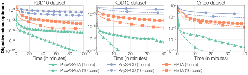
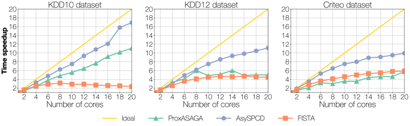
Figure 1: Convergence for asynchronous stochastic methods for $\ell_{1}+\ell_{2}$-regularized logistic regression. Top: Suboptimality as a function of time for different asynchronous methods using 1 and 10 cores. Bottom: Running time speedup as function of the number of cores. ProxAsaga achieves significant speedups over its sequential version while being orders of magnitude faster than competing methods. AsySpcd achieves the highest speedups but it also the slowest overall method.

Results.

We compare three parallel asynchronous methods on the aforementioned datasets: ProxAsaga (this work), AsySpcd, the asynchronous proximal coordinate descent method of Liu & Wright (2015) and the (synchronous) Fista algorithm (Beck & Teboulle, 2009), in which the gradient computation is parallelized by splitting the dataset into equal batches. We aim to benchmark these methods in the most realistic scenario possible; to this end we use the following step size: $1/2L$ for ProxAsaga, $1/L_{c}$ for AsySpcd, where $L_{c}$ is the coordinate-wise Lipschitz constant of the gradient, while Fista uses backtracking line-search. The results can be seen in Figure 1 (top) with both one (thus sequential) and ten processors. Two main observations can be made from this figure. First, ProxAsaga is significantly faster on these problems. Second, its asynchronous version offers a significant speedup over its sequential counterpart.

In Figure 1 (bottom) we present speedup with respect to the number of cores, where speedup is computed as the time to achieve a suboptimality of $10^{-10}$ with one core divided by the time to achieve the same suboptimality using several cores. While our theoretical speedups (with respect to the number of iterations) are almost linear as our theory predicts (see Appendix F), we observe a different story for our running time speedups. This can be attributed to memory access overhead, which our model does not take into account. As predicted by our theoretical results, we observe a high correlation between the $\Delta$ dataset sparsity measure and the empirical speedup: KDD 2010 ($\Delta=0.15$) achieves a 11x speedup, while in Criteo ($\Delta=0.89$) the speedup is never above 6x.

Note that although competitor methods exhibit similar or sometimes better speedups, they remain orders of magnitude slower than ProxAsaga in running time for large sparse problems. In fact, our method is between 5x and 80x times faster (in time to reach $10^{-10}$ suboptimality) than Fista and between 13x and 290x times faster than AsySpcd (see Appendix F.3).

5 Conclusion and future work

In this work, we have described ProxAsaga, an asynchronous variance reduced algorithm with support for composite objective functions. This method builds upon a novel sparse variant of the (proximal) Saga algorithm that takes advantage of sparsity in the individual gradients. We have proven that this algorithm is linearly convergent under a condition on the step size and that it is linearly faster than its sequential counterpart given a bound on the delay. Empirical benchmarks show that ProxAsaga is orders of magnitude faster than existing state-of-the-art methods.

This work can be extended in several ways. First, we have focused on the Saga method as the basic iteration loop, but this approach can likely be extended to other proximal incremental schemes such as Sgd or ProxSvrg. Second, as mentioned in §3.3, it is an open question whether it is possible to obtain convergence guarantees without any sparsity assumption, as was done for Asaga.

Breaking the Nonsmooth Barrier: A Scalable Parallel Method for Composite Optimization

Supplementary material

Notations.

Throughout the supplementary material we use the following extra notation. We denote by $\langle\cdot,\cdot\rangle_{(i)}$ (resp. $\|\cdot\|_{(i)}$) the scalar product (resp. norm) restricted to blocks in $T_{i}$, i.e., $\langle{\boldsymbol{x}},{\boldsymbol{y}}\rangle_{(i)}:=\sum_{B\in T_{i}}\langle[{\boldsymbol{x}}]_{B},[{\boldsymbol{y}}]_{B}\rangle$ and $\|{\boldsymbol{x}}\|_{(i)}:=\sqrt{\langle{\boldsymbol{x}},{\boldsymbol{x}}\rangle_{(i)}}$. We will also use the following definitions: $\varphi:=\sum_{B\in\mathcal{B}}d_{B}h_{B}({\boldsymbol{x}})$ and ${\boldsymbol{D}}$ is the diagonal matrix defined block-wise as $[{\boldsymbol{D}}]_{B,B}=d_{B}\boldsymbol{I}_{|B|}$.

The Bregman divergence associated with a convex function $f$ for points ${\boldsymbol{x}},{\boldsymbol{y}}$ in its domain is defined as:

$$B_{f}({\boldsymbol{x}},{\boldsymbol{y}}):=f({\boldsymbol{x}})-f({\boldsymbol{y}})-\langle\nabla f({\boldsymbol{y}}),{\boldsymbol{x}}-{\boldsymbol{y}}\rangle\,.$$ (7)

Note that this is always positive due to the convexity of $f$.

Appendix Appendix A Basic properties

Lemma 1.

For any $\mu$-strongly convex function $f$ we have the following inequality:

$$\langle\nabla f({\boldsymbol{y}})-\nabla f({\boldsymbol{x}}),{\boldsymbol{y}}-{\boldsymbol{x}}\rangle\geq\frac{\mu}{2}\|{\boldsymbol{y}}-{\boldsymbol{x}}\|^{2}+B_{f}({\boldsymbol{x}},{\boldsymbol{y}})\,.$$ (8)

Proof.

By strong convexity, $f$ verifies the inequality:

$$f({\boldsymbol{y}})\leq f({\boldsymbol{x}})+\langle\nabla f({\boldsymbol{y}}),{\boldsymbol{y}}-{\boldsymbol{x}}\rangle-\frac{\mu}{2}\|{\boldsymbol{y}}-{\boldsymbol{x}}\|^{2}\,,$$ (9)

for any ${\boldsymbol{x}},{\boldsymbol{y}}$ in the domain (see e.g. (Nesterov, 2004)). We then have the equivalences:

$$\qquad f({\boldsymbol{x}})\leq f({\boldsymbol{y}})+\langle\nabla f({\boldsymbol{x}}),{\boldsymbol{x}}-{\boldsymbol{y}}\rangle-\frac{\mu}{2}\|{\boldsymbol{x}}-{\boldsymbol{y}}\|^{2}$$

$$\iff\frac{\mu}{2}\|{\boldsymbol{x}}-{\boldsymbol{y}}\|^{2}+f({\boldsymbol{x}})-f({\boldsymbol{y}})\leq\langle\nabla f({\boldsymbol{x}}),{\boldsymbol{x}}-{\boldsymbol{y}}\rangle$$

$$\iff\frac{\mu}{2}\|{\boldsymbol{x}}-{\boldsymbol{y}}\|^{2}+\underbrace{f({\boldsymbol{x}})-f({\boldsymbol{y}})-\langle\nabla f({\boldsymbol{y}}),{\boldsymbol{x}}-{\boldsymbol{y}}\rangle}_{B_{f}({\boldsymbol{x}},{\boldsymbol{y}})}\leq\langle\nabla f({\boldsymbol{x}})-\nabla f({\boldsymbol{y}}),{\boldsymbol{x}}-{\boldsymbol{y}}\rangle\,,$$ (10)

where in the last line we have subtracted $\langle\nabla f({\boldsymbol{y}}),{\boldsymbol{x}}-{\boldsymbol{y}}\rangle$ from both sides of the inequality. ∎

Lemma 2.

Let the $f_{i}$ be $L$-smooth and convex functions. Then it is verified that:

$$\frac{1}{n}\sum_{i=1}^{n}\|\nabla f_{i}({\boldsymbol{x}})-\nabla f_{i}({\boldsymbol{y}})\|^{2}\leq 2LB_{f}({\boldsymbol{x}},{\boldsymbol{y}})\,.$$ (11)

Proof.

Since each $f_{i}$ is $L$-smooth, it is verified (see e.g. Nesterov (2004, Theorem 2.1.5)) that

$$\|\nabla f_{i}({\boldsymbol{x}})-\nabla f_{i}({\boldsymbol{y}})\|^{2}\leq 2L\big{(}f_{i}({\boldsymbol{x}})-f_{i}({\boldsymbol{y}})-\langle\nabla f_{i}({\boldsymbol{y}}),{\boldsymbol{x}}-{\boldsymbol{y}}\rangle\big{)}\,.$$ (12)

The result is obtained by averaging over $i$. ∎

Lemma 3 (Characterization of the proximal operator).

Let $h$ be convex lower semicontinuous. Then we have the following characterization of the proximal operator:

$${\boldsymbol{z}}={\mathbf{prox}}_{\gamma h}({\boldsymbol{x}})\iff\frac{1}{\gamma}({\boldsymbol{x}}-{\boldsymbol{z}})\in\partial h({\boldsymbol{z}})\,.$$ (13)

Proof.

This is a direct consequence of the first order optimality conditions on the definition of proximal operator, see e.g. (Beck & Teboulle, 2009; Nesterov, 2013). ∎

Lemma 4 (Firm non-expansiveness).

Let ${\boldsymbol{x}},\tilde{{\boldsymbol{x}}}$ be two arbitrary elements in the domain of $\varphi_{i}$ and ${\boldsymbol{z}},\tilde{{\boldsymbol{z}}}$ be defined as ${\boldsymbol{z}}:={\emph{\text{prox}}}_{\varphi_{i}}({\boldsymbol{x}})$, $\tilde{{\boldsymbol{z}}}:={\emph{\text{prox}}}_{\varphi_{i}}(\tilde{{\boldsymbol{x}}})$. Then it is verified that:

$$\langle{\boldsymbol{z}}-\tilde{{\boldsymbol{z}}},{\boldsymbol{x}}-\tilde{{\boldsymbol{x}}}\rangle_{(i)}\geq\|{\boldsymbol{z}}-\tilde{{\boldsymbol{z}}}\|_{(i)}^{2}\,.$$ (14)

Proof.

By the block-separability of $\varphi_{i}$, the proximal operator is the concatenation of the proximal operators of the blocks. In other words, for any block $B\in T_{i}$ we have:

$$[{\boldsymbol{z}}]_{B}={\mathbf{prox}}_{\gamma\varphi_{B}}([{\boldsymbol{x}}]_{B})~{},\quad[\tilde{{\boldsymbol{z}}}]_{B}={\mathbf{prox}}_{\gamma\varphi_{B}}([\tilde{{\boldsymbol{x}}}]_{B})\,,$$ (15)

where $\varphi_{B}$ is the restriction of $\varphi_{i}$ to $B$. By firm non-expansiveness of the proximal operator (see e.g. Bauschke & Combettes (2011, Proposition 4.2)) we have that:

$$\langle[{\boldsymbol{z}}]_{B}-[\tilde{{\boldsymbol{z}}}]_{B},[{\boldsymbol{x}}]_{B}-[\tilde{{\boldsymbol{x}}}]_{B}\rangle\geq\|[{\boldsymbol{z}}]_{B}-[\tilde{{\boldsymbol{z}}}]_{B}\|^{2}\,.$$

Summing over the blocks in $T_{i}$ yields the desired result. ∎

Appendix Appendix B Sparse Proximal SAGA

This Appendix contains all proofs for Section 2. The main result of this section is Theorem 1, whose proof is structured as follows:

• We start by proving four auxiliary results that will be used later on in the proofs of both synchronous and asynchronous variants. The first is the unbiasedness of key quantities used in the algorithm. The second is a characterization of the solutions of (OPT) in terms of $f$ and $\varphi$ (defined below) in Lemma 6. The third is a key inequality in Lemma 7 that relates the gradient mapping to other terms that arise in the optimization. The fourth is an upper bound on the variance terms of the gradient estimator, relating it to the Bregman divergence of $f$ and the past gradient estimator terms.

• In Lemma 9, we define an upper bound on the iterates $\|{\boldsymbol{x}}_{t}-{\boldsymbol{x}}^{*}\|^{2}$, called a Lyapunov function, and prove an inequality that relates this Lyapunov function value at the current iterate with its value at the previous iterate.

• Finally, in the proof of Theorem 1 we use the previous inequality in terms of the Lyapunov function to prove a geometric convergence of the iterates.

We start by proving the following unbiasedness result, mentioned in §2.

Lemma 5.

Let ${\boldsymbol{D}}_{i}$ and $\varphi_{i}$ be defined as in §2. Then it is verified that $\mathbf{E}{\boldsymbol{D}}_{i}=\boldsymbol{I}_{p}$ and $\mathbf{E}\,\varphi_{i}=h$.

Proof.

Let $B\in\mathcal{B}$ an arbitrary block. We have the following sequence of equalities:

$$\mathbf{E}[{\boldsymbol{D}}_{i}]_{B,B} =\frac{1}{n}\sum_{i=1}^{n}[{\boldsymbol{D}}_{i}]_{B,B}=\frac{1}{n}\sum_{i=1}^{n}d_{B}\mathds{1}\{B\in T_{i}\}\boldsymbol{I}_{|B|}$$ (16)

$$=\frac{1}{n}\sum_{i=1}^{n}\frac{n}{n_{B}}\mathds{1}\{B\in T_{i}\}\boldsymbol{I}_{|B|}$$ (17)

$$=\left(\frac{1}{n_{B}}\sum_{i=1}^{n}\mathds{1}\{B\in T_{i}\}\right)\boldsymbol{I}_{|B|}=\boldsymbol{I}_{|B|}~{},$$ (18)

where the last equality comes from the definition of $n_{B}$. $\mathbf{E}{\boldsymbol{D}}_{i}=\boldsymbol{I}_{p}$ then follows from the arbitrariness of $B$.

Similarly, for $\varphi_{i}$ we have:

$$\mathbf{E}\varphi_{i}([{\boldsymbol{x}}]_{B}) =\frac{1}{n}\sum_{i=1}^{n}d_{B}\mathds{1}\{B\in T_{i}\}h_{B}([{\boldsymbol{x}}]_{B})$$ (19)

$$=\frac{1}{n}\sum_{i=1}^{n}\frac{n}{n_{B}}\mathds{1}\{B\in T_{i}\}h_{B}([{\boldsymbol{x}}]_{B})$$ (20)

$$=\left(\frac{1}{n_{B}}\sum_{i=1}^{n}\mathds{1}\{B\in T_{i}\}\right)h_{B}([{\boldsymbol{x}}]_{B})=h_{B}([{\boldsymbol{x}}]_{B})~{},$$ (21)

Finally, the result $\mathbf{E}\,\varphi_{i}=h$ comes from adding over all blocks. ∎

Lemma 6.

${\boldsymbol{x}}^{*}$ is a solution to (OPT) if and only if the following condition is verified:

$${\boldsymbol{x}}^{*}={\mathbf{prox}}_{\gamma\varphi}\big{(}{\boldsymbol{x}}^{*}-\gamma\boldsymbol{{\boldsymbol{D}}}\nabla f({\boldsymbol{x}}^{*})\big{)}\,.$$ (22)

Proof.

By the first order optimality conditions, the solutions to (OPT) are characterized by the subdifferential inclusion ${-\nabla f({\boldsymbol{x}}^{*})\in\partial h({\boldsymbol{x}}^{*})}$. We can then write the following sequence of equivalences:

$$-\nabla f({\boldsymbol{x}}^{*})\in\partial h({\boldsymbol{x}}^{*}) \iff-{\boldsymbol{D}}\nabla f({\boldsymbol{x}}^{*})\in{\boldsymbol{D}}\partial h({\boldsymbol{x}}^{*})$$

(multiplying by $${\boldsymbol{D}}$$, equivalence since diagonals are nonzero)

$$\iff-{\boldsymbol{D}}\nabla f({\boldsymbol{x}}^{*})\in\partial\varphi({\boldsymbol{x}}^{*})$$

(by definition of $$\varphi$$)

$$\iff\mfrac{1}{\gamma}({\boldsymbol{x}}^{*}-\gamma{\boldsymbol{D}}\nabla f({\boldsymbol{x}}^{*})-{\boldsymbol{x}}^{*})\in\partial\varphi({\boldsymbol{x}}^{*}$$

(adding and subtracting $${\boldsymbol{x}}^{*}$$)

$$\iff{\boldsymbol{x}}^{*}={\mathbf{prox}}_{\gamma\varphi}({\boldsymbol{x}}^{*}-\gamma{\boldsymbol{D}}\nabla f({\boldsymbol{x}}^{*}))\,.$$ (23)

(by Lemma 3)

Since all steps are equivalences, we have the desired result. ∎

The following lemma will be key in the proof of convergence for both the sequential and the parallel versions of the algorithm. With this result, we will be able to bound the product between the gradient mapping and the iterate suboptimality by:

• First, the negative norm of the gradient mapping, which will be key in the parallel setting to cancel out the terms arising from the asynchrony.

• Second, variance terms in $\|{\boldsymbol{v}}_{i}-{\boldsymbol{D}}_{i}\nabla f({\boldsymbol{x}}^{*})\|^{2}$ that we will be able to bound by the Bregman divergence using Lemma 2.

• Third and last, a product with terms in $\langle{\boldsymbol{v}}_{i}-{\boldsymbol{D}}_{i}\nabla f({\boldsymbol{x}}^{*}),{\boldsymbol{x}}-{\boldsymbol{x}}^{*}\rangle$, which taken in expectation gives $\langle\nabla f({\boldsymbol{x}})-\nabla f({\boldsymbol{x}}^{*}),{\boldsymbol{x}}-{\boldsymbol{x}}^{*}\rangle$ and will allow us to apply Lemma 1 to obtain the contraction terms needed to obtain a geometric rate of convergence.

Lemma 7 (Gradient mapping inequality).

Let ${\boldsymbol{x}}$ be an arbitrary vector, ${\boldsymbol{x}}^{*}$ a solution to (OPT), ${\boldsymbol{v}}_{i}$ as defined in (SPS) and $\boldsymbol{g}=\boldsymbol{g}({\boldsymbol{x}},{\boldsymbol{v}}_{i},i)$ the gradient mapping defined in (3). Then the following inequality is verified for any $\beta>0$:

$$\langle\boldsymbol{g},{\boldsymbol{x}}-{\boldsymbol{x}}^{*}\rangle\geq-\frac{\gamma}{2}(\beta-2)\|\boldsymbol{g}\|^{2}-\frac{\gamma}{2\beta}\|{\boldsymbol{v}}_{i}-{\boldsymbol{D}}_{i}\nabla f({\boldsymbol{x}}^{*})\|^{2}+\langle{\boldsymbol{v}}_{i}-{\boldsymbol{D}}_{i}\nabla f({\boldsymbol{x}}^{*}),{\boldsymbol{x}}-{\boldsymbol{x}}^{*}\rangle\,.$$ (24)

Proof.

By firm non-expansiveness of the proximal operator (Lemma 4) applied to ${\boldsymbol{z}}={\mathbf{prox}}_{\gamma\varphi_{i}}({\boldsymbol{x}}-\gamma{\boldsymbol{v}}_{i})$ and $\tilde{{\boldsymbol{z}}}={\mathbf{prox}}_{\gamma\varphi_{i}}({\boldsymbol{x}}^{*}-\gamma{\boldsymbol{D}}\nabla f({\boldsymbol{x}}^{*}))$ we have:

$$\|{\boldsymbol{z}}-\tilde{\boldsymbol{z}}\|_{(i)}^{2}-\langle{\boldsymbol{z}}-\tilde{\boldsymbol{z}},{\boldsymbol{x}}-\gamma{\boldsymbol{v}}_{i}-{\boldsymbol{x}}^{*}+\gamma{\boldsymbol{D}}\nabla f({\boldsymbol{x}}^{*})\rangle_{(i)}\leq 0~{}.$$ (25)

By the (SPS) iteration we have ${\boldsymbol{x}}^{+}={\boldsymbol{z}}$ and by Lemma 3 we have that $[{\boldsymbol{z}}]_{T_{i}}=[{\boldsymbol{x}}^{*}]_{T_{i}}$, hence the above can be rewritten as

$$\|{\boldsymbol{x}}^{+}-{\boldsymbol{x}}^{*}\|_{(i)}^{2}-\langle{\boldsymbol{x}}^{+}-{\boldsymbol{x}}^{*},{\boldsymbol{x}}-\gamma{\boldsymbol{v}}_{i}-{\boldsymbol{x}}^{*}+\gamma{\boldsymbol{D}}\nabla f({\boldsymbol{x}}^{*})\rangle_{(i)}\leq 0~{}.$$ (26)

We can now write the following sequence of inequalities

$$\langle\gamma\boldsymbol{g},{\boldsymbol{x}}-{\boldsymbol{x}}^{*}\rangle=\langle{\boldsymbol{x}}-{\boldsymbol{x}}^{+},{\boldsymbol{x}}-{\boldsymbol{x}}^{*}\rangle_{(i)}\qquad\text{ (by definition and sparsity of $g$)}$$

$$\qquad=\langle{\boldsymbol{x}}-{\boldsymbol{x}}^{+}+{\boldsymbol{x}}^{*}-{\boldsymbol{x}}^{*},{\boldsymbol{x}}-{\boldsymbol{x}}^{*}\rangle_{(i)}$$

$$\qquad=\|{\boldsymbol{x}}-{\boldsymbol{x}}^{*}\|_{(i)}^{2}-\langle{\boldsymbol{x}}^{+}-{\boldsymbol{x}}^{*},{\boldsymbol{x}}-{\boldsymbol{x}}^{*}\rangle_{(i)}$$

$$\qquad\geq\|{\boldsymbol{x}}-{\boldsymbol{x}}^{*}\|_{(i)}^{2}-\langle{\boldsymbol{x}}^{+}-{\boldsymbol{x}}^{*},2{\boldsymbol{x}}-\gamma{\boldsymbol{v}}_{i}-2{\boldsymbol{x}}^{*}+\gamma{\boldsymbol{D}}\nabla f({\boldsymbol{x}}^{*})\rangle_{(i)}+\|{\boldsymbol{x}}^{+}-{\boldsymbol{x}}^{*}\|^{2}_{(i)}$$ (27)

(adding Eq. (26))

$$\qquad=\|{\boldsymbol{x}}-{\boldsymbol{x}}^{+}\|_{(i)}^{2}+\langle{\boldsymbol{x}}^{+}-{\boldsymbol{x}}^{*},\gamma{\boldsymbol{v}}_{i}-\gamma{\boldsymbol{D}}\nabla f({\boldsymbol{x}}^{*})\rangle_{(i)}\qquad\text{ (completing the square)}$$

$$\qquad=\|{\boldsymbol{x}}-{\boldsymbol{x}}^{+}\|_{(i)}^{2}+\langle{\boldsymbol{x}}-{\boldsymbol{x}}^{*},\gamma{\boldsymbol{v}}_{i}-\gamma{\boldsymbol{D}}\nabla f({\boldsymbol{x}}^{*})\rangle_{(i)}-\langle{\boldsymbol{x}}-{\boldsymbol{x}}^{+},\gamma{\boldsymbol{v}}_{i}-\gamma{\boldsymbol{D}}\nabla f({\boldsymbol{x}}^{*})\rangle_{(i)}$$

(adding and substracting $${\boldsymbol{x}}$$)

$$\qquad\geq\Big{(}1-\frac{\beta}{2}\Big{)}\|{\boldsymbol{x}}-{\boldsymbol{x}}^{+}\|_{(i)}^{2}-\frac{\gamma^{2}}{2\beta}\|{\boldsymbol{v}}_{i}-{\boldsymbol{D}}\nabla f({\boldsymbol{x}}^{*})\|_{(i)}^{2}+\gamma\langle{\boldsymbol{v}}_{i}-{\boldsymbol{D}}\nabla f({\boldsymbol{x}}^{*}),{\boldsymbol{x}}-{\boldsymbol{x}}^{*}\rangle_{(i)}$$

(Young’s inequality $${2\langle a,b\rangle\leq\frac{\|a\|^{2}}{\beta}+\beta\|b\|^{2}} \beta>0$$, valid for arbitrary )

$$\qquad\geq\Big{(}1-\frac{\beta}{2}\Big{)}\|{\boldsymbol{x}}-{\boldsymbol{x}}^{+}\|_{(i)}^{2}-\frac{\gamma^{2}}{2\beta}\|{\boldsymbol{v}}_{i}-{\boldsymbol{D}}_{i}\nabla f({\boldsymbol{x}}^{*})\|^{2}+\gamma\langle{\boldsymbol{v}}_{i}-{\boldsymbol{D}}_{i}\nabla f({\boldsymbol{x}}^{*}),{\boldsymbol{x}}-{\boldsymbol{x}}^{*}\rangle$$

(by definition of $${\boldsymbol{D}}_{i} {\boldsymbol{v}}_{i} T_{i}$$ and using the fact that is -sparse)

$$\qquad=\Big{(}1-\frac{\beta}{2}\Big{)}\|\gamma\boldsymbol{g}\|^{2}-\frac{\gamma^{2}}{2\beta}\|{\boldsymbol{v}}_{i}-{\boldsymbol{D}}_{i}\nabla f({\boldsymbol{x}}^{*})\|^{2}+\gamma\langle{\boldsymbol{v}}_{i}-{\boldsymbol{D}}\nabla f({\boldsymbol{x}}^{*}),{\boldsymbol{x}}-{\boldsymbol{x}}^{*}\rangle\,,$$ (28)

where in the last inequality we have used the fact that $\boldsymbol{g}$ is $T_{i}$-sparse. Finally, dividing by $\gamma$ both sides yields the desired result. ∎

Lemma 8 (Upper bound on the gradient estimator variance).

For arbitrary vectors ${\boldsymbol{x}}$, $({\boldsymbol{\alpha}}_{i})_{i=0}^{n}$, and ${\boldsymbol{v}}_{i}$ as defined in (SPS) we have:

$$\mathbf{E}\|{\boldsymbol{v}}_{i}-{\boldsymbol{D}}_{i}\nabla f({\boldsymbol{x}}^{*})\|^{2}\leq 4LB_{f}({\boldsymbol{x}},{\boldsymbol{x}}^{*})+2\mathbf{E}\|{\boldsymbol{\alpha}}_{i}-\nabla f_{i}({\boldsymbol{x}}^{*})\|^{2}\,.$$ (29)

Proof.

We will now bound the variance terms. For this we have:

$$\mathbf{E}\|{\boldsymbol{v}}_{i}-{\boldsymbol{D}}\nabla f({\boldsymbol{x}}^{*})\|_{(i)}^{2}=\mathbf{E}\|\nabla f_{i}({\boldsymbol{x}})-\nabla f_{i}({\boldsymbol{x}}^{*})+\nabla f_{i}({\boldsymbol{x}}^{*})-{\boldsymbol{\alpha}}_{i}+{\boldsymbol{D}}_{i}\overline{{\boldsymbol{\alpha}}}-{\boldsymbol{D}}\nabla f({\boldsymbol{x}}^{*})\|_{(i)}^{2}$$

$$\qquad\leq 2\mathbf{E}\|\nabla f_{i}({\boldsymbol{x}})-\nabla f_{i}({\boldsymbol{x}}^{*})\|^{2}+2\mathbf{E}\|\nabla f_{i}({\boldsymbol{x}}^{*})-{\boldsymbol{\alpha}}_{i}-({\boldsymbol{D}}\nabla f({\boldsymbol{x}}^{*})-{\boldsymbol{D}}\overline{{\boldsymbol{\alpha}}})\|_{(i)}^{2}$$

(by inequality $$\|a+b\|^{2}\leq 2\|a\|^{2}+2\|b\|^{2}$$)

$$\qquad=2\mathbf{E}\|\nabla f_{i}({\boldsymbol{x}})-\nabla f_{i}({\boldsymbol{x}}^{*})\|^{2}+2\mathbf{E}\|\nabla f_{i}({\boldsymbol{x}}^{*})-{\boldsymbol{\alpha}}_{i}\|^{2}$$

$$\qquad\qquad-4\mathbf{E}\langle\nabla f_{i}({\boldsymbol{x}}^{*})-{\boldsymbol{\alpha}}_{i},{\boldsymbol{D}}\nabla f({\boldsymbol{x}}^{*})-{\boldsymbol{D}}\overline{{\boldsymbol{\alpha}}}\rangle_{(i)}+2\mathbf{E}\|{\boldsymbol{D}}\nabla f({\boldsymbol{x}}^{*})-{\boldsymbol{D}}\overline{{\boldsymbol{\alpha}}}\|_{(i)}^{2}\,.$$ (30)

(developing the square)

We will now simplify the last two terms in the above expression. For the first of the two last terms we have:

$$-4\mathbf{E}\langle\nabla f_{i}({\boldsymbol{x}}^{*})-{\boldsymbol{\alpha}}_{i},{\boldsymbol{D}}\nabla f({\boldsymbol{x}}^{*})-{\boldsymbol{D}}\overline{{\boldsymbol{\alpha}}}\rangle_{(i)}=-4\mathbf{E}\langle\nabla f_{i}({\boldsymbol{x}}^{*})-{\boldsymbol{\alpha}}_{i},{\boldsymbol{D}}\nabla f({\boldsymbol{x}}^{*})-{\boldsymbol{D}}\overline{{\boldsymbol{\alpha}}}\rangle$$ (31)

(support of first term)

$$\qquad=-4\langle\nabla f({\boldsymbol{x}}^{*})-\overline{{\boldsymbol{\alpha}}},{\boldsymbol{D}}\nabla f({\boldsymbol{x}}^{*})-{\boldsymbol{D}}\overline{{\boldsymbol{\alpha}}}\rangle$$

$$\qquad=-4\|\nabla f({\boldsymbol{x}}^{*})-\overline{{\boldsymbol{\alpha}}}\|_{{\boldsymbol{D}}}^{2}\,.$$ (32)

Similarly, for the last term we have:

$$2\mathbf{E}\|{\boldsymbol{D}}\nabla f({\boldsymbol{x}}^{*})-{\boldsymbol{D}}\overline{{\boldsymbol{\alpha}}}\|_{(i)}^{2} =2\mathbf{E}\langle{\boldsymbol{D}}_{i}\nabla f({\boldsymbol{x}}^{*})-{\boldsymbol{D}}_{i}\overline{{\boldsymbol{\alpha}}},{\boldsymbol{D}}\nabla f({\boldsymbol{x}}^{*})-{\boldsymbol{D}}\overline{{\boldsymbol{\alpha}}}\rangle$$

$$=2\langle\nabla f({\boldsymbol{x}}^{*})-\overline{{\boldsymbol{\alpha}}},{\boldsymbol{D}}\nabla f({\boldsymbol{x}}^{*})-{\boldsymbol{D}}\overline{{\boldsymbol{\alpha}}}\rangle$$

(using Lemma 5)

$$=2\|\nabla f({\boldsymbol{x}}^{*})-\overline{{\boldsymbol{\alpha}}}\|_{{\boldsymbol{D}}}^{2}\,.$$ (33)

and so the addition of these terms is negative and can be dropped. In all, for the variance terms we have

$$\mathbf{E}\|{\boldsymbol{v}}_{i}-{\boldsymbol{D}}\nabla f({\boldsymbol{x}}^{*})\|_{(i)}^{2} \leq 2\mathbf{E}\|\nabla f_{i}({\boldsymbol{x}})-\nabla f_{i}({\boldsymbol{x}}^{*})\|^{2}+2\mathbf{E}\|{\boldsymbol{\alpha}}_{i}-\nabla f_{i}({\boldsymbol{x}}^{*})\|^{2}$$

$$\leq 4LB_{f}({\boldsymbol{x}},{\boldsymbol{x}}^{*})+2\mathbf{E}\|{\boldsymbol{\alpha}}_{i}-\nabla f_{i}({\boldsymbol{x}}^{*})\|^{2}\,.\qquad\text{ (by Lemma~{}\ref{lemma:l_smooth_ineq}) }$$ (34)

∎

We now define an upper bound on the quantity that we would like to bound, often called a Lyapunov function, and establish a recursive inequality on this Lyapunov function.

Lemma 9 (Lyapunov inequality).

Let $\mathcal{L}$ be the following $c$-parametrized function:

$$\mathcal{L}({\boldsymbol{x}},{\boldsymbol{\alpha}}):=\|{\boldsymbol{x}}-{\boldsymbol{x}}^{*}\|^{2}+\frac{c}{n}\sum_{i=1}^{n}\|{\boldsymbol{\alpha}}_{i}-\nabla f_{i}({\boldsymbol{x}}^{*})\|^{2}\,.$$ (35)

Let ${\boldsymbol{x}}^{+}$ and ${\boldsymbol{\alpha}}^{+}$ be obtained from the Sparse Proximal Saga updates (SPS). Then we have:

$$\mathbf{E}\mathcal{L}({\boldsymbol{x}}^{+},{\boldsymbol{\alpha}}^{+})-\mathcal{L}({\boldsymbol{x}},{\boldsymbol{\alpha}})\leq -\gamma\mu\|{\boldsymbol{x}}-{\boldsymbol{x}}^{*}\|^{2}+\left(4L\gamma^{2}-2\gamma+2L\frac{c}{n}\right)B_{f}({\boldsymbol{x}},{\boldsymbol{x}}^{*})$$

$$+\left(2\gamma^{2}-\frac{c}{n}\right)\mathbf{E}\|{\boldsymbol{\alpha}}_{i}-\nabla f_{i}({\boldsymbol{x}})\|^{2}\,.$$ (36)

Proof.

For the first term of $\mathcal{L}$ we have:

$$\|{\boldsymbol{x}}^{+}-{\boldsymbol{x}}^{*}\|^{2} =\|{\boldsymbol{x}}-\gamma\boldsymbol{g}-{\boldsymbol{x}}^{*}\|^{2}\qquad\text{ ($\boldsymbol{g}:=\boldsymbol{g}({\boldsymbol{x}},{\boldsymbol{v}}_{i},i)$)}$$

$$=\|{\boldsymbol{x}}-{\boldsymbol{x}}^{*}\|^{2}-2\gamma\langle\boldsymbol{g},{\boldsymbol{x}}-{\boldsymbol{x}}^{*}\rangle+\|\gamma\boldsymbol{g}\|^{2}$$

$$\leq\|{\boldsymbol{x}}-{\boldsymbol{x}}^{*}\|^{2}+\gamma^{2}\|{\boldsymbol{v}}_{i}-{\boldsymbol{D}}_{i}\nabla f({\boldsymbol{x}}^{*})\|^{2}-2\gamma\langle{\boldsymbol{v}}_{i}-{\boldsymbol{D}}_{i}\nabla f({\boldsymbol{x}}^{*}),{\boldsymbol{x}}-{\boldsymbol{x}}^{*}\rangle$$

(by Lemma 7 with $$\beta=1$$)

Since ${\boldsymbol{v}}_{i}$ is an unbiased estimator of the gradient and $\mathbf{E}{\boldsymbol{D}}_{i}=\boldsymbol{I}_{p}$, taking expectations we have:

$$\mathbf{E}\|{\boldsymbol{x}}^{+}-{\boldsymbol{x}}^{*}\|^{2} \leq\|{\boldsymbol{x}}-{\boldsymbol{x}}^{*}\|^{2}+\gamma^{2}\mathbf{E}\|{\boldsymbol{v}}_{i}-{\boldsymbol{D}}_{i}\nabla f({\boldsymbol{x}}^{*})\|^{2}-2\gamma\langle\nabla f({\boldsymbol{x}})-\nabla f({\boldsymbol{x}}^{*}),{\boldsymbol{x}}-{\boldsymbol{x}}^{*}\rangle$$ (38)

$$\leq(1-\gamma\mu)\|{\boldsymbol{x}}-{\boldsymbol{x}}^{*}\|^{2}+\gamma^{2}\mathbf{E}\|{\boldsymbol{v}}_{i}-{\boldsymbol{D}}_{i}\nabla f({\boldsymbol{x}}^{*})\|^{2}-2\gamma B_{f}({\boldsymbol{x}},{\boldsymbol{x}}^{*})\,.$$

       (by Lemma 1)

By using the variance terms bound (Lemma 8) in the previous equation we have:

$$\mathbf{E}\|{\boldsymbol{x}}^{+}-{\boldsymbol{x}}^{*}\|^{2} \leq(1-\gamma\mu)\|{\boldsymbol{x}}-{\boldsymbol{x}}^{*}\|^{2}+(4L\gamma^{2}-2\gamma)B_{f}({\boldsymbol{x}},{\boldsymbol{x}}^{*})$$ (39)

$$\qquad+2\gamma^{2}\mathbf{E}\|{\boldsymbol{\alpha}}_{i}-\nabla f_{i}({\boldsymbol{x}}^{*})\|^{2}\,.$$

We will now bound the second term of the Lyapunov function. We have:

$$\frac{1}{n}\sum_{i=1}^{n}\|{\boldsymbol{\alpha}}_{i}^{+}-\nabla f_{i}({\boldsymbol{x}}^{*})\|^{2} =\left(1-\frac{1}{n}\right)\mathbf{E}\|{\boldsymbol{\alpha}}_{i}-\nabla f_{i}({\boldsymbol{x}}^{*})\|^{2}+\frac{1}{n}\mathbf{E}\|\nabla f_{i}({\boldsymbol{x}})-\nabla f_{i}({\boldsymbol{x}}^{*})\|^{2}$$

(by definition of $${\boldsymbol{\alpha}}^{+}$$) (40)

$$\leq\left(1-\frac{1}{n}\right)\mathbf{E}\|{\boldsymbol{\alpha}}_{i}-\nabla f_{i}({\boldsymbol{x}}^{*})\|^{2}+\frac{2}{n}LB_{f}({\boldsymbol{x}},{\boldsymbol{x}}^{*})\,.\quad\text{ (by Lemma~{}\ref{lemma:l_smooth_ineq})}$$ (41)

Combining Eq. (39) and (Appendix B) we have:

$$\mathbf{E}\mathcal{L}({\boldsymbol{x}}^{+},{\boldsymbol{\alpha}}^{+}) \leq(1-\gamma\mu)\|{\boldsymbol{x}}-{\boldsymbol{x}}^{*}\|^{2}+(4L\gamma^{2}-2\gamma)B_{f}({\boldsymbol{x}},{\boldsymbol{x}}^{*})+2\gamma^{2}\mathbf{E}\|{\boldsymbol{\alpha}}_{i}-\nabla f_{i}({\boldsymbol{x}}^{*})\|^{2}$$

$$\qquad+c\left[\left(1-\frac{1}{n}\right)\mathbf{E}\|{\boldsymbol{\alpha}}_{i}-\nabla f_{i}({\boldsymbol{x}}^{*})\|^{2}+\frac{1}{n}2LB_{f}({\boldsymbol{x}},{\boldsymbol{x}}^{*})\right]$$

$$=(1-\gamma\mu)\|{\boldsymbol{x}}-{\boldsymbol{x}}^{*}\|^{2}+\left(4L\gamma^{2}-2\gamma+2L\frac{c}{n}\right)B_{f}({\boldsymbol{x}},{\boldsymbol{x}}^{*})$$

$$\qquad+\left(2\gamma^{2}-\frac{c}{n}\right)\mathbf{E}\|{\boldsymbol{\alpha}}_{i}-\nabla f_{i}({\boldsymbol{x}}^{*})\|^{2}+c\mathbf{E}\|{\boldsymbol{\alpha}}_{i}-\nabla f_{i}({\boldsymbol{x}}^{*})\|^{2}$$

$$=\mathcal{L}({\boldsymbol{x}},{\boldsymbol{\alpha}})-\gamma\mu\|{\boldsymbol{x}}-{\boldsymbol{x}}^{*}\|^{2}+\left(4L\gamma^{2}-2\gamma+2L\frac{c}{n}\right)B_{f}({\boldsymbol{x}},{\boldsymbol{x}}^{*})$$

$$\qquad+\left(2\gamma^{2}-\frac{c}{n}\right)\mathbf{E}\|{\boldsymbol{\alpha}}_{i}-\nabla f_{i}({\boldsymbol{x}}^{*})\|^{2}\,.$$ (42)

Finally, subtracting $\mathcal{L}({\boldsymbol{x}},{\boldsymbol{\alpha}})$ from both sides yields the desired result. ∎

Theorem 1.

Let $\gamma=\frac{a}{5L}$ for any $a\leq 1$ and $f$ be $\mu$-strongly convex. Then Sparse Proximal Saga converges geometrically in expectation with a rate factor of at least $\rho=\frac{1}{5}\min\{\frac{1}{n},a\frac{1}{\kappa}\}$. That is, for ${\boldsymbol{x}}_{t}$ obtained after $t$ updates and ${\boldsymbol{x}}^{*}$ the solution to (OPT), we have the bound:

$${\mathbb{E}}\|{\boldsymbol{x}}_{t}-{\boldsymbol{x}}^{*}\|^{2}\leq(1-\rho)^{t}C_{0}\,,\quad\text{ with }C_{0}:=\|{\boldsymbol{x}}_{0}-{\boldsymbol{x}}^{*}\|^{2}+\textstyle\frac{1}{5L^{2}}\sum_{i=1}^{n}\|{\boldsymbol{\alpha}}_{i}^{0}-\nabla f_{i}({\boldsymbol{x}}^{*})\|^{2}\quad.$$

Proof.

Let $\overline{H}:=\frac{1}{n}\sum_{i}\|{\boldsymbol{\alpha}}_{i}-\nabla f_{i}({\boldsymbol{x}}^{*})\|^{2}$. By the Lyapunov inequality from Lemma 9, we have:

$$\mathbf{E}\mathcal{L}_{t+1}-(1-\rho)\mathcal{L}_{t}\leq\rho\mathcal{L}_{t}-\gamma\mu\|{\boldsymbol{x}}_{t}-{\boldsymbol{x}}^{*}\|^{2}+\left(4L\gamma^{2}-2\gamma+2L\frac{c}{n}\right)B_{f}({\boldsymbol{x}}_{t},{\boldsymbol{x}}^{*})+\left(2\gamma^{2}-\frac{c}{n}\right)\overline{H}$$

$$\qquad=\left(\rho-\gamma\mu\right)\|{\boldsymbol{x}}_{t}-{\boldsymbol{x}}^{*}\|^{2}+\left(4L\gamma^{2}-2\gamma+2L\frac{c}{n}\right)B_{f}({\boldsymbol{x}}_{t},{\boldsymbol{x}}^{*})+\left[2\gamma^{2}+c\left(\rho-\frac{1}{n}\right)\right]\overline{H}$$

(by definition of $$\mathcal{L}_{t}$$)

$$\qquad\leq\left(\rho-\gamma\mu\right)\|{\boldsymbol{x}}_{t}-{\boldsymbol{x}}^{*}\|^{2}+\left(4L\gamma^{2}-2\gamma+2L\frac{c}{n}\right)B_{f}({\boldsymbol{x}}_{t},{\boldsymbol{x}}^{*})+\left(2\gamma^{2}-\frac{2c}{3n}\right)\overline{H}$$

(choosing $$\rho\leq\frac{1}{3n}$$)

$$\qquad=\left(\rho-\gamma\mu\right)\|{\boldsymbol{x}}_{t}-{\boldsymbol{x}}^{*}\|^{2}+\left(10L\gamma^{2}-2\gamma\right)B_{f}({\boldsymbol{x}}_{t},{\boldsymbol{x}}^{*})$$

(choosing $$\frac{c}{n}=3\gamma^{2}$$)

$$\qquad\leq\left(\rho-\frac{a\mu}{5L}\right)\|{\boldsymbol{x}}_{t}-{\boldsymbol{x}}^{*}\|^{2}\qquad\text{ (for all $\gamma=\frac{a}{5L},a\leq 1$)}$$

$$\qquad\leq 0\,.\qquad\text{ (for $\rho\leq\frac{a}{5}\cdot\frac{\mu}{L}$)}$$ (43)

And so we have the bound:

$$\mathbf{E}\mathcal{L}_{t+1}\leq\left(1-\min\Big{\{}\frac{1}{3n},\frac{a}{5}\cdot\frac{1}{\kappa}\Big{\}}\right)\mathcal{L}_{t}\leq\left(1-\frac{1}{5}\min\Big{\{}\frac{1}{n},a\cdot\frac{1}{\kappa}\Big{\}}\right)\mathcal{L}_{t}\,,$$ (44)

where in the last inequality we have used the trivial bound $\frac{1}{3n}\leq\frac{1}{5n}$ merely for clarity of exposition. Chaining expectations from $t$ to $0$ we have:

$${\mathbb{E}}\mathcal{L}_{t+1} \leq\left(1-\frac{1}{5}\min\Big{\{}\frac{1}{n},a\cdot\frac{1}{\kappa}\Big{\}}\right)^{t+1}\mathcal{L}_{0}$$

$$=\left(1-\frac{1}{5}\min\Big{\{}\frac{1}{n},a\cdot\frac{1}{\kappa}\Big{\}}\right)^{t+1}\left(\|{\boldsymbol{x}}_{0}-{\boldsymbol{x}}^{*}\|^{2}+\frac{3a^{2}}{5^{2}L^{2}}\sum_{i=1}^{n}\|{\boldsymbol{\alpha}}_{i}^{0}-\nabla f_{i}({\boldsymbol{x}}^{*})\|^{2}\right)$$

$$\leq\left(1-\frac{1}{5}\min\Big{\{}\frac{1}{n},a\cdot\frac{1}{\kappa}\Big{\}}\right)^{t+1}\left(\|{\boldsymbol{x}}_{0}-{\boldsymbol{x}}^{*}\|^{2}+\frac{1}{5L^{2}}\sum_{i=1}^{n}\|{\boldsymbol{\alpha}}_{i}^{0}-\nabla f_{i}({\boldsymbol{x}}^{*})\|^{2}\right)$$ (45)

$$\qquad\text{ (since $a\leq 1$ and $\nicefrac{{3}}{{5}}\leq 1$)}\,.$$

The fact that $\mathcal{L}_{t}$ is a majorizer of $\|{\boldsymbol{x}}_{t}-{\boldsymbol{x}}^{*}\|^{2}$ completes the proof. ∎

Appendix Appendix C ProxASAGA

In this Appendix we provide the proofs for results from Section 3, that is Theorem 2 (the convergence theorem for ProxAsaga) and Corollary 1 (its speedup result).

Notation.

Through this section, we use the following shorthand for the gradient mapping: $\boldsymbol{g}_{t}:=\boldsymbol{g}(\hat{{\boldsymbol{x}}}_{t},\hat{{\boldsymbol{v}}}^{t}_{i_{t}},i_{t})$.

Appendix C.1 Proof outline.

As in the smooth case ($h=0$), we start by using the definition of ${\boldsymbol{x}}_{t+1}$ in Eq. (4) to relate the distance to the optimum in terms of its previous iterates:

$$\|{\boldsymbol{x}}_{t+1}-{\boldsymbol{x}}^{*}\|^{2}= \|{\boldsymbol{x}}_{t}-{\boldsymbol{x}}^{*}\|^{2}+2\gamma\langle\hat{\boldsymbol{x}}_{t}-{\boldsymbol{x}}_{t},\boldsymbol{g}_{t}\rangle+\gamma^{2}\|\boldsymbol{g}_{t}\|^{2}-2\gamma\langle\hat{\boldsymbol{x}}_{t}-{\boldsymbol{x}}^{*},\boldsymbol{g}_{t}\rangle\,.$$ (46)

However, in this case $\boldsymbol{g}_{t}$ is not a gradient estimator but a gradient mapping, so we cannot continue as is customary – by using the unbiasedness of the gradient in the $\langle\hat{\boldsymbol{x}}_{t}-{\boldsymbol{x}}^{*},\boldsymbol{g}_{t}\rangle$ term together with the strong convexity of $f$ (see Leblond et al. (2017, Section 3.5)).

To circumvent this difficulty, we derive a tailored inequality for the gradient mapping (Lemma 7 in Appendix B), which in turn allows us to use the classical unbiasedness and strong convexity arguments to get the following inequality:

$$a_{t+1}\leq(1-\frac{\gamma\mu}{2})a_{t}+\gamma^{2} {\mathbb{E}}\|\boldsymbol{g}_{t}\|^{2}-2\gamma{\mathbb{E}}B_{f}(\hat{{\boldsymbol{x}}}_{t},{\boldsymbol{x}}^{*})+\underbrace{\gamma\mu{\mathbb{E}}\|\hat{{\boldsymbol{x}}}_{t}-{\boldsymbol{x}}\|^{2}+2\gamma{\mathbb{E}}\langle\boldsymbol{g}_{t},\hat{{\boldsymbol{x}}}_{t}-{\boldsymbol{x}}_{t}\rangle}_{\text{additional asynchrony terms}}$$ (47)

$$\underbrace{+\gamma^{2}(\beta-2){\mathbb{E}}\|\boldsymbol{g}_{t}\|^{2}+\frac{\gamma^{2}}{\beta}{\mathbb{E}}\|\hat{\boldsymbol{v}}^{t}_{i_{t}}-{\boldsymbol{D}}_{i_{t}}\nabla f({\boldsymbol{x}}^{*})\|^{2}}_{\text{additional proximal and variance terms}}\,,$$

where $a_{t}:={\mathbb{E}}\|{\boldsymbol{x}}_{t}-{\boldsymbol{x}}^{*}\|^{2}$. Note that since $f$ is strongly convex, $B_{f}(\hat{{\boldsymbol{x}}}_{t},{\boldsymbol{x}}^{*})\geq\frac{\mu}{2}\|\hat{\boldsymbol{x}}_{t}-{\boldsymbol{x}}^{*}\|^{2}$.

In the smooth setting, one first expresses the additional asynchrony terms as linear combinations of past gradient variance terms $({\mathbb{E}}\|\boldsymbol{g}_{u}\|^{2})_{0\leq u\leq t}$. Then one crucially uses the negative Bregman divergence term to control the variance terms. However, in our current setting, we cannot relate the norm of the gradient mapping ${\mathbb{E}}\|\boldsymbol{g}_{t}\|^{2}$ to the Bregman divergence (from which $h$ is absent). Instead, we use the negative term $\gamma^{2}(\beta-1){\mathbb{E}}\|\boldsymbol{g}_{t}\|^{2}$ to control all the $({\mathbb{E}}\|\boldsymbol{g}_{u}\|^{2})_{0\leq u\leq t}$ terms that arise from asynchrony.

The rest of the proof consists in:

$i)$ expressing the additional asynchrony terms as linear combinations of $({\mathbb{E}}\|\boldsymbol{g}_{u}\|^{2})_{0\leq u\leq t}$, following Leblond et al. (2017, Lemma 1);

$ii)$ expressing the last variance term, $\|\hat{\boldsymbol{v}}^{t}_{i_{t}}-D_{i_{t}}\nabla f({\boldsymbol{x}}^{*})\|^{2}$, as a linear combination of past Bregman divergences (Lemma 8 in Appendix B and Lemma 2 from Leblond et al. (2017));

$iii)$ defining a Lyapunov function, $\mathcal{L}_{t}:={\sum_{u=0}^{t}(1-\rho)^{t-u}a_{u}}$, and proving that it is bounded by a contraction given conditions on the maximum step size and delay.

Appendix C.2 Detailed proof

Theorem 2 (Convergence guarantee and rate of ProxAsaga).

Suppose $\tau\leq\frac{1}{10\sqrt{\Delta}}$. For any step size $\gamma=\frac{a}{L}$ with $a\leq\frac{1}{36}\min\{1,\frac{6\kappa}{\tau}\}$, the inconsistent read iterates of Algorithm 1 converge in expectation at a geometric rate factor of at least: $\rho(a)=\frac{1}{5}\min\big{\{}\frac{1}{n},a\frac{1}{\kappa}\big{\}},$ i.e. ${\mathbb{E}}\|\hat{\boldsymbol{x}}_{t}-{\boldsymbol{x}}^{*}\|^{2}\leq(1-\rho)^{t}\,\tilde{C}_{0}$, where $\tilde{C}_{0}$ is a constant independent of $t$ ($\approx\frac{n\kappa}{a}C_{0}$ with $C_{0}$ as defined in Theorem 1).

Proof.

In order to get an initial recursive inequality, we first unroll the (virtual) update:

$$\|{\boldsymbol{x}}_{t+1}-{\boldsymbol{x}}^{*}\|^{2} =\|{\boldsymbol{x}}_{t}-\gamma\boldsymbol{g}_{t}-{\boldsymbol{x}}^{*}\|^{2}=\|{\boldsymbol{x}}_{t}-{\boldsymbol{x}}^{*}\|^{2}+\|\gamma\boldsymbol{g}_{t}\|^{2}-2\gamma\langle\boldsymbol{g}_{t},{\boldsymbol{x}}_{t}-{\boldsymbol{x}}^{*}\rangle$$

$$=\|{\boldsymbol{x}}_{t}-{\boldsymbol{x}}^{*}\|^{2}+\|\gamma\boldsymbol{g}_{t}\|^{2}-2\gamma\langle\boldsymbol{g}_{t},\hat{{\boldsymbol{x}}}_{t}-{\boldsymbol{x}}^{*}\rangle+2\gamma\langle\boldsymbol{g}_{t},\hat{{\boldsymbol{x}}}_{t}-{\boldsymbol{x}}_{t}\rangle\,,$$ (48)

and then apply Lemma 7 with ${\boldsymbol{x}}=\hat{\boldsymbol{x}}_{t}$ and ${\boldsymbol{v}}=\hat{{\boldsymbol{v}}}_{i_{t}}^{t}$. Note that in this case we have $\boldsymbol{g}=\boldsymbol{g}_{t}$ and $\langle\cdot\rangle_{(i)}=\langle\cdot\rangle_{(i_{t})}$.

$$\|{\boldsymbol{x}}_{t+1}-{\boldsymbol{x}}^{*}\|^{2} \leq\|{\boldsymbol{x}}_{t}-{\boldsymbol{x}}^{*}\|^{2}+2\gamma\langle\boldsymbol{g}_{t},\hat{{\boldsymbol{x}}}_{t}-{\boldsymbol{x}}_{t}\rangle+\gamma^{2}\|\boldsymbol{g}_{t}\|^{2}+\gamma^{2}(\beta-2)\|\boldsymbol{g}_{t}\|^{2}$$

$$\qquad+\frac{\gamma^{2}}{\beta}\|\hat{{\boldsymbol{v}}}_{i_{t}}^{t}-{\boldsymbol{D}}\nabla f({\boldsymbol{x}}^{*})\|_{({i_{t}})}^{2}-2\gamma\langle\hat{{\boldsymbol{v}}}_{i_{t}}^{t}-{\boldsymbol{D}}\nabla f({\boldsymbol{x}}^{*}),\hat{{\boldsymbol{x}}}_{t}-{\boldsymbol{x}}^{*}\rangle_{({i_{t}})}$$

$$=\|{\boldsymbol{x}}_{t}-{\boldsymbol{x}}^{*}\|^{2}+2\gamma\langle\boldsymbol{g}_{t},\hat{{\boldsymbol{x}}}_{t}-{\boldsymbol{x}}_{t}\rangle+\gamma^{2}(\beta-1)\|\boldsymbol{g}_{t}\|^{2}$$

$$\qquad+\frac{\gamma^{2}}{\beta}\|\hat{{\boldsymbol{v}}}_{i_{t}}^{t}-{\boldsymbol{D}}_{i_{t}}\nabla f({\boldsymbol{x}}^{*})\|^{2}-2\gamma\langle\hat{{\boldsymbol{v}}}_{i_{t}}^{t}-{\boldsymbol{D}}_{i_{t}}\nabla f({\boldsymbol{x}}^{*}),\hat{{\boldsymbol{x}}}_{t}-{\boldsymbol{x}}^{*}\rangle.$$ (49)

(as $${[\hat{{\boldsymbol{v}}}_{i_{t}}^{t}]_{T_{i_{t}}}}=\hat{{\boldsymbol{v}}}_{i_{t}}^{t}$$)

We now use the property that $i_{t}$ is independent of $\hat{\boldsymbol{x}}_{t}$ (which we enforce by reading $\hat{\boldsymbol{x}}_{t}$ before picking $i_{t}$, see Section 3), together with the unbiasedness of the gradient update $\hat{{\boldsymbol{v}}}_{i_{t}}^{t}$ ($\mathbf{E}\hat{{\boldsymbol{v}}}_{i_{t}}^{t}=\nabla f(\hat{{\boldsymbol{x}}}_{t})$) and the definition of ${\boldsymbol{D}}$ to simplify the following expression as follows:

$$\mathbf{E}\langle\hat{{\boldsymbol{v}}}_{i_{t}}^{t}-{\boldsymbol{D}}_{i_{t}}\nabla f({\boldsymbol{x}}^{*}),\hat{{\boldsymbol{x}}}_{t}-{\boldsymbol{x}}^{*}\rangle =\langle\nabla f(\hat{{\boldsymbol{x}}}_{t})-\nabla f({\boldsymbol{x}}^{*}),\hat{{\boldsymbol{x}}}_{t}-{\boldsymbol{x}}^{*}\rangle$$

$$\geq\frac{\mu}{2}\|\hat{{\boldsymbol{x}}}_{t}-{\boldsymbol{x}}^{*}\|^{2}+B_{f}(\hat{{\boldsymbol{x}}}_{t},{\boldsymbol{x}}^{*})\,,$$ (50)

where the last inequality comes from Lemma 1. Taking conditional expectations on (Appendix C.2) we get:

$$\mathbf{E}\|{\boldsymbol{x}}_{t+1}-{\boldsymbol{x}}^{*}\|^{2} \leq\|{\boldsymbol{x}}_{t}-{\boldsymbol{x}}^{*}\|^{2}+2\gamma\mathbf{E}\langle\boldsymbol{g}_{t},\hat{{\boldsymbol{x}}}_{t}-{\boldsymbol{x}}_{t}\rangle+\gamma^{2}(\beta-1)\mathbf{E}\|\boldsymbol{g}_{t}\|^{2}$$ (51)

$$\qquad+\frac{\gamma^{2}}{\beta}\mathbf{E}\|\hat{{\boldsymbol{v}}}_{i_{t}}^{t}-{\boldsymbol{D}}_{i_{t}}\nabla f({\boldsymbol{x}}^{*})\|^{2}-\gamma\mu\|\hat{{\boldsymbol{x}}}_{t}-{\boldsymbol{x}}^{*}\|^{2}-2\gamma B_{f}(\hat{{\boldsymbol{x}}}_{t},{\boldsymbol{x}}^{*})$$

$$\leq(1-\frac{\gamma\mu}{2})\|{\boldsymbol{x}}_{t}-{\boldsymbol{x}}^{*}\|^{2}+2\gamma\mathbf{E}\langle\boldsymbol{g}_{t},\hat{{\boldsymbol{x}}}_{t}-{\boldsymbol{x}}_{t}\rangle+\gamma^{2}(\beta-1)\mathbf{E}\|\boldsymbol{g}_{t}\|^{2}$$

$$\qquad+\frac{\gamma^{2}}{\beta}\mathbf{E}\|\hat{{\boldsymbol{v}}}_{i_{t}}^{t}-{\boldsymbol{D}}_{i_{t}}\nabla f({\boldsymbol{x}}^{*})\|^{2}+\gamma\mu\|\hat{{\boldsymbol{x}}}_{t}-{\boldsymbol{x}}_{t}\|^{2}-2\gamma B_{f}(\hat{{\boldsymbol{x}}}_{t},{\boldsymbol{x}}^{*})$$

(using $$\|a+b\|^{2}\leq 2\|a\|^{2}+2\|b\|^{2} \|{\boldsymbol{x}}_{t}-\hat{{\boldsymbol{x}}}_{t}+\hat{{\boldsymbol{x}}}_{t}-{\boldsymbol{x}}^{*}\|^{2}$$ on )

$$\leq(1-\frac{\gamma\mu}{2})\|{\boldsymbol{x}}_{t}-{\boldsymbol{x}}^{*}\|^{2}+\gamma^{2}(\beta-1)\mathbf{E}\|\boldsymbol{g}_{t}\|^{2}+\gamma\mu\|\hat{{\boldsymbol{x}}}_{t}-{\boldsymbol{x}}_{t}\|^{2}+2\gamma\mathbf{E}\langle\boldsymbol{g}_{t},\hat{{\boldsymbol{x}}}_{t}-{\boldsymbol{x}}_{t}\rangle$$

$$\qquad-2\gamma B_{f}(\hat{{\boldsymbol{x}}}_{t},{\boldsymbol{x}}^{*})+\frac{4\gamma^{2}L}{\beta}B_{f}(\hat{{\boldsymbol{x}}}_{t},{\boldsymbol{x}}^{*})+\frac{2\gamma^{2}}{\beta}\mathbf{E}\|\hat{{\boldsymbol{\alpha}}}^{t}_{i_{t}}-\nabla f_{i_{t}}({\boldsymbol{x}}^{*})\|^{2}\,.$$ (52)

(using Lemma 8 on the variance terms)

Since we also have:

$$\hat{\boldsymbol{x}}_{t}-{\boldsymbol{x}}_{t}=\gamma\sum_{u=(t-\tau)_{+}}^{t-1}\boldsymbol{G}_{u}^{t}\boldsymbol{g}(\hat{\boldsymbol{x}}_{u},\hat{\boldsymbol{\alpha}}^{u},i_{u}),$$ (53)

the effect of asynchrony for the perturbed iterate updates was already derived in a very similar setup in Leblond et al. (2017). We re-use the following bounds from their Appendix C.4:

$${\mathbb{E}}\|\hat{{\boldsymbol{x}}}_{t}-{\boldsymbol{x}}_{t}\|^{2}\leq\gamma^{2}(1+\sqrt{\Delta}\tau)\sum_{u=(t-\tau)_{+}}^{t-1}{\mathbb{E}}\|\boldsymbol{g}_{u}\|^{2}\,,$$ Leblond et al. (2017, Eq. (48)) (54)

$${\mathbb{E}}\langle\boldsymbol{g}_{t},\hat{{\boldsymbol{x}}}_{t}-{\boldsymbol{x}}_{t}\rangle\leq\frac{\gamma\sqrt{\Delta}}{2}\sum_{u=(t-\tau)_{+}}^{t-1}{\mathbb{E}}\|\boldsymbol{g}_{u}\|^{2}+\frac{\gamma\sqrt{\Delta}\tau}{2}{\mathbb{E}}\|\boldsymbol{g}_{t}\|^{2}\,. \text{\cite[citet]{\@@bibref{Authors Phrase1YearPhrase2}{leblond2016Asaga}{\@@citephrase{(}}{\@@citephrase{, Eq.~{}(46))}}}}.$$ (55)

Because the updates on ${\boldsymbol{\alpha}}$ are the same for ProxAsaga as for Asaga, we can re-use the same argument arising in the proof of Leblond et al. (2017, Lemma 2) to get the following bound on ${\mathbb{E}}\|\hat{{\boldsymbol{\alpha}}}^{t}_{i_{t}}-\nabla f_{i_{t}}({\boldsymbol{x}}^{*})\|^{2}$:

$${\mathbb{E}}\|\hat{{\boldsymbol{\alpha}}}^{t}_{i_{t}}-\nabla f_{i_{t}}({\boldsymbol{x}}^{*})\|^{2}\leq\frac{2L}{n}\underbrace{\sum_{u=1}^{t-1}(1-\frac{1}{n})^{(t-2\tau-u-1)_{+}}{\mathbb{E}}B_{f}(\hat{{\boldsymbol{x}}}_{u},{\boldsymbol{x}}^{*})}_{\text{Henceforth denoted $H_{t}$}}+2L(1-\frac{1}{n})^{(t-\tau)_{+}}\tilde{e}_{0}\,,$$ (56)

where $\tilde{e}_{0}:=\frac{1}{2L}{\mathbb{E}}\|{\boldsymbol{\alpha}}_{i}^{0}-f^{\prime}_{i}({\boldsymbol{x}}^{*})\|^{2}$. This bound is obtained by analyzing which gradient could be the source of ${\boldsymbol{\alpha}}_{i_{t}}$ in the past (taking in consideration the inconsistent writes), and then applying Lemma 2 on the $\mathbf{E}\|\nabla f(\hat{{\boldsymbol{x}}}_{u})-\nabla f({\boldsymbol{x}}^{*})\|^{2}$ terms, explaining the presence of $B_{f}(\hat{{\boldsymbol{x}}}_{u},{\boldsymbol{x}}^{*})$ terms. The inequality (56) corresponds to Eq. (56) and (57) in Leblond et al. (2017).

By taking the full expectation of (52) and plugging the above inequalities back, we obtain an inequality similar to Leblond et al. (2017, Master inequality (28)) which describes how the error terms $a_{t}:={\mathbb{E}}\|{\boldsymbol{x}}_{t}-{\boldsymbol{x}}^{*}\|^{2}$ of the virtual iterates are related:

$$a_{t+1}\leq (1-\frac{\gamma\mu}{2})a_{t}+\frac{4\gamma^{2}L}{\beta}(1-\frac{1}{n})^{(t-\tau)_{+}}\tilde{e}_{0}$$ (57)

$$+\gamma^{2}\left[\beta-1+\sqrt{\Delta}\tau\right]{\mathbb{E}}\|\boldsymbol{g}_{t}\|^{2}+\left[\gamma^{2}\sqrt{\Delta}+\gamma^{3}\mu(1+\sqrt{\Delta}\tau)\right]\sum_{u=(t-\tau)_{+}}^{t}{\mathbb{E}}\|\boldsymbol{g}_{u}\|^{2}$$

$$-2\gamma{\mathbb{E}}B_{f}(\hat{{\boldsymbol{x}}}_{t},{\boldsymbol{x}}^{*})+\frac{4\gamma^{2}L}{\beta}{\mathbb{E}}B_{f}(\hat{{\boldsymbol{x}}}_{t},{\boldsymbol{x}}^{*})+\frac{4\gamma^{2}L}{\beta n}H_{t}\,.$$

We now have a promising inequality with a contractive term and several quantities that we need to bound. In order to achieve our final result, we introduce the same Lyapunov function as in Leblond et al. (2017):

$$\mathcal{L}_{t}:=\sum_{u=0}^{t}(1-\rho)^{t-u}a_{u}\,,$$

where $\rho$ is a target rate factor for which we will provide a value later on. Proving that this Lyapunov function is bounded by a contraction will finish our proof. We have:

$$\mathcal{L}_{t+1}=\sum_{u=0}^{t+1}(1-\rho)^{t+1-u}a_{u} =(1-\rho)^{t+1}a_{0}+\sum_{u=1}^{t+1}(1-\rho)^{t+1-u}a_{u}$$

$$=(1-\rho)^{t+1}a_{0}+\sum_{u=0}^{t}(1-\rho)^{t-u}a_{u+1}\,.$$ (58)

We now plug our new bound on $a_{t+1}$, (57):

$$\mathcal{L}_{t+1}\leq(1-\rho)^{t+1}a_{0}+\sum_{u=0}^{t}(1-\rho)^{t-u}\Big{[} (1-\frac{\gamma\mu}{2})a_{u}+\frac{4\gamma^{2}L}{\beta}(1-\frac{1}{n})^{(u-\tau)_{+}}\tilde{e}_{0}$$ (59)

$$+\gamma^{2}\big{(}\beta-1+\sqrt{\Delta}\tau\big{)}{\mathbb{E}}\|\boldsymbol{g}_{u}\|^{2}$$

$$+\big{(}\gamma^{2}\sqrt{\Delta}+\gamma^{3}\mu(1+\sqrt{\Delta}\tau)\big{)}\sum_{v=(u-\tau)_{+}}^{u}{\mathbb{E}}\|\boldsymbol{g}_{v}\|^{2}$$

$$-2\gamma{\mathbb{E}}B_{f}(\hat{{\boldsymbol{x}}}_{u},{\boldsymbol{x}}^{*})+\frac{4\gamma^{2}L}{\beta}{\mathbb{E}}B_{f}(\hat{{\boldsymbol{x}}}_{u},{\boldsymbol{x}}^{*})+\frac{4\gamma^{2}L}{\beta n}H_{u}\Big{]}\,.$$

After regrouping similar terms, we get:

$$\mathcal{L}_{t+1}\leq(1-\rho)^{t+1}(a_{0}+A\tilde{e}_{0})+(1-\frac{\gamma\mu}{2})\mathcal{L}_{t}+\sum_{u=0}^{t}s_{u}^{t}{\mathbb{E}}\|\boldsymbol{g}_{u}\|^{2}+\sum_{u=1}^{t}r_{u}^{t}{\mathbb{E}}B_{f}(\hat{{\boldsymbol{x}}}_{u},{\boldsymbol{x}}^{*})\,.$$ (60)

Now, provided that we can prove that under certain conditions the $s_{u}^{t}$ and $r_{u}^{t}$ terms are all negative (and that the $A$ term is not too big), we can drop them from the right-hand side of (60) which will allow us to finish the proof.

Let us compute these terms. Let $q:=\frac{1-\nicefrac{{1}}{{n}}}{1-\rho}$ and we assume in the rest that $\rho<\nicefrac{{1}}{{n}}$.

Computing $A$. We have:

$$\frac{4\gamma^{2}L}{\beta}\sum_{u=0}^{t}(1-\rho)^{t-u}(1-\frac{1}{n})^{(u-\tau)_{+}} \leq\frac{4\gamma^{2}L}{\beta}(1-\rho)^{t}(1-\rho)^{-\tau}(\tau+1+\frac{1}{1-q})$$

from Leblond et al. (2017, Eq (75))

$$=(1-\rho)^{t+1}\underbrace{\frac{4\gamma^{2}L}{\beta}(1-\rho)^{-\tau-1}(\tau+1+\frac{1}{1-q})}_{:=A}\,.$$ (61)

Computing $s_{u}^{t}$. Since we have:

$$\sum_{u=0}^{t}(1-\rho)^{t-u}\sum_{v=(u-\tau)_{+}}^{u-1}{\mathbb{E}}\|\boldsymbol{g}_{u}\|^{2}\leq\tau(1-\rho)^{-\tau}\sum_{u=0}^{t}(1-\rho)^{t-u}{\mathbb{E}}\|\boldsymbol{g}_{u}\|^{2}\,,$$ (62)

we have for all $0\leq u\leq t$:

$$s_{u}^{t}\leq(1-\rho)^{t-u}\Big{[}\gamma^{2}\big{(}\beta-1+\sqrt{\Delta}\tau)+\tau(1-\rho)^{-\tau}\big{(}\gamma^{2}\sqrt{\Delta}+\gamma^{3}\mu(1+\sqrt{\Delta}\tau)\big{)}\Big{]}\,.$$ (63)

Computing $r_{u}^{t}$. To analyze these quantities, we need to compute: $\sum_{u=0}^{t}(1-\rho)^{t-u}\sum_{v=1}^{u-1}(1-\frac{1}{n})^{(u-2\tau-v-1)_{+}}$. Fortunately, this is already done in Leblond et al. (2017, Eq (66)), and thus we know that for all $1\leq u\leq t$:

$$r_{u}^{t}\leq(1-\rho)^{t-u}\left[-2\gamma+\frac{4\gamma^{2}L}{\beta}+\frac{4L\gamma^{2}}{n\beta}(1-\rho)^{-2\tau-1}\Big{(}2\tau+\frac{1}{1-q}\Big{)}\right]\,,$$ (64)

recalling that $q:=\frac{1-\nicefrac{{1}}{{n}}}{1-\rho}$ and that we assumed $\rho<\frac{1}{n}$.

We now need some assumptions to further analyze these quantities. We make simple choices for simplicity, though a tighter analysis is possible. To get manageable (and simple) constants, we follow Leblond et al. (2017, Eq. (82) and (83)) and assume:

$$\rho\leq\frac{1}{4n};\quad\tau\leq\frac{n}{10}\,.$$ (65)

This tells us:

$$\frac{1}{1-q} \leq\frac{4n}{3}$$

$$(1-\rho)^{-k\tau-1} \leq\frac{4}{3}\qquad\qquad\text{for}\,\,0\leq k\leq 2\,.\qquad\text{(using Bernouilli's inequality)}$$

Additionally, we set $\beta=\frac{1}{2}$. Equation (63) thus becomes:

$$s_{u}^{t}\leq\gamma^{2}(1-\rho)^{t-u}\left[-\frac{1}{2}+\sqrt{\Delta}\tau+\frac{4}{3}\big{(}\sqrt{\Delta}\tau+\gamma\mu\tau(1+\sqrt{\Delta}\tau)\big{)}\right]\,.$$ (66)

We see that for $s_{u}^{t}$ to be negative, we need $\tau=\mathcal{O}(\frac{1}{\sqrt{\Delta}})$. Let us assume that $\tau\leq\frac{1}{10\sqrt{\Delta}}$. We then get:

$$s_{u}^{t}\leq\gamma^{2}(1-\rho)^{t-u}\left[-\frac{1}{2}+\frac{1}{10}+\frac{4}{30}+\gamma\mu\tau\frac{4}{3}\frac{11}{10}\right]\,.$$ (67)

Thus, the condition under which all $s_{u}^{t}$ are negative boils down to:

$$\gamma\mu\tau\leq\frac{2}{11}\,.$$ (68)

Now looking at the $r_{u}^{t}$ terms given our assumptions, the inequality (64) becomes:

$$r_{u}^{t} \leq(1-\rho)^{t-u}\left[-2\gamma+8\gamma^{2}L+\frac{8\gamma^{2}L}{n}\frac{4}{3}\big{(}\frac{n}{5}+\frac{4n}{3}\big{)}\right]$$

$$\leq(1-\rho)^{t-u}\big{(}-2\gamma+36\gamma^{2}L\big{)}\,.$$ (69)

The condition for all $r_{u}^{t}$ to be negative then can be simplified down to:

$$\gamma\leq\frac{1}{18L}\,.$$ (70)

We now have a promising inequality for proving that our Lyapunov function is bounded by a contraction. However we have defined $\mathcal{L}_{t}$ in terms of the virtual iterate ${\boldsymbol{x}}_{t}$, which means that our result would only hold for a given $T$ fixed in advance, as is the case in Mania et al. (2017). Fortunately, we can use the same trick as in Leblond et al. (2017, Eq. (97)): we simply add $\gamma B_{f}(\hat{\boldsymbol{x}}_{t},{\boldsymbol{x}}^{*})$ to both sides in (60). $r_{t}^{t}$ is replaced by $r_{t}^{t}+\gamma$, which makes for a slightly worse bound on $\gamma$ to ensure linear convergence:

$$\gamma\leq\frac{1}{36L}\,.$$ (71)

For this small cost, we get a contraction bound on $B_{f}(\hat{\boldsymbol{x}}_{t},{\boldsymbol{x}}^{*})$, and thus by the strong convexity of $f$ (see (9)) we get a contraction bound for ${\mathbb{E}}\|\hat{\boldsymbol{x}}_{t}-{\boldsymbol{x}}^{*}\|^{2}$.

Recap. Let us use $\rho=\frac{1}{4n}$ and $\gamma:=\frac{a}{L}$. Then the conditions (68) and (71) on the step size $\gamma$ reduce to:

$$a\leq\frac{1}{36}\min\{1,\frac{72}{11}\frac{\kappa}{\tau}\}.$$ (72)

Moreover, the condition:

$$\tau\leq\frac{1}{10\sqrt{\Delta}}$$ (73)

is sufficient to also ensure that (65) is satisfied as $\Delta\in[\frac{1}{n},1]$, and thus $\frac{1}{\sqrt{\Delta}}\leq\sqrt{n}\leq n$.

Thus under the conditions (72) and (73), we have that all $s_{u}^{t}$ and $r_{u}^{t}$ terms are negative and we can rewrite the recurrent step of our Lyapunov function as:

$$\mathcal{L}_{t+1}\leq\gamma{\mathbb{E}}B_{f}(\hat{{\boldsymbol{x}}}_{t})+\mathcal{L}_{t+1}\leq(1-\rho)^{t+1}(a_{0}+A\tilde{e}_{0})+(1-\frac{\gamma\mu}{2})\mathcal{L}_{t}\,.$$ (74)

By unrolling the recursion (74), we can carefully combine the effect of the geometric term $(1-\rho)$ with the one of $(1-\frac{\gamma\mu}{2})$. This was already done in Leblond et al. (2017, Apx C.9, Eq. (101) to (103)), with a trick to handle various boundary cases, yielding the overall rate:

$${\mathbb{E}}B_{f}(\hat{\boldsymbol{x}}_{t},{\boldsymbol{x}}^{*})\leq(1-\rho^{*})^{t+1}\hat{C}_{0},$$ (75)

where $\rho^{*}=\min\{\frac{1}{5n},a\frac{2}{5\kappa}\}$ (that we simplified to $\rho^{*}=\frac{1}{5}\min\{\frac{1}{n},a\frac{1}{\kappa}\}$ in the theorem statement). To get the final constant, we need to bound $A$. We have:

$$A =\frac{4\gamma^{2}L}{\beta}(1-\rho)^{-\tau-1}(\tau+1+\frac{1}{1-q})$$

$$\leq 8\gamma^{2}L\frac{4}{3}(\frac{n}{10}+1+\frac{4n}{3})$$

$$\leq 26\gamma^{2}Ln$$

$$\leq\gamma n\,.$$ (76)

This is the same bound on $A$ that was used by Leblond et al. (2017) and so we obtain the same constant as their Eq. (104):

$$\hat{C}_{0}:=\frac{21n}{\gamma}(\|{\boldsymbol{x}}_{0}-{\boldsymbol{x}}^{*}\|^{2}+\gamma\frac{n}{2L}{\mathbb{E}}\|{\boldsymbol{\alpha}}_{i}^{0}-\nabla f_{i}({\boldsymbol{x}}^{*})\|^{2}).$$ (77)

Note that $\hat{C}_{0}=\mathcal{O}(\frac{n}{\gamma}C_{0})$ with $C_{0}$ defined as in Theorem 1.

Now, using the strong convexity of $f$ via (9), we get:

$${\mathbb{E}}\|\hat{\boldsymbol{x}}_{t}-{\boldsymbol{x}}^{*}\|^{2}\leq\frac{2}{\mu}{\mathbb{E}}B_{f}(\hat{\boldsymbol{x}}_{t},{\boldsymbol{x}}^{*})\leq(1-\rho^{*})^{t+1}\tilde{C}_{0},$$ (78)

where $\tilde{C_{0}}=\mathcal{O}(\frac{n\kappa}{a}C_{0})$.

This finishes the proof for Theorem 2. ∎

Corollary 3 (Speedup).

Suppose $\tau\leq\frac{1}{10\sqrt{\Delta}}$. If $\kappa\geq n$, then using the step size $\gamma=\nicefrac{{1}}{{36L}}$, ProxAsaga converges geometrically with rate factor $\Omega(\frac{1}{\kappa})$. If $\kappa<n$, then using the step size $\gamma=\nicefrac{{1}}{{36n\mu}}$, ProxAsaga converges geometrically with rate factor $\Omega(\frac{1}{n})$. In both cases, the convergence rate is the same as Sparse Proximal Saga and ProxAsaga is thus linearly faster than its sequential counterpart up to a constant factor. Note that in both cases the step size does not depend on $\tau$.

Furthermore, if $\tau\leq 6\kappa$, we can use a universal step size of $\Theta(\nicefrac{{1}}{{L}})$ to get a similar rate for ProxAsaga than Sparse Proximal Saga, thus making it adaptive to local strong convexity since the knowledge of $\kappa$ is not required.

Proof.

If $\kappa\geq n$, the rate factor of Sparse Proximal Saga is $\nicefrac{{1}}{{\kappa}}$. To get the same rate factor, we need to choose $a=\Omega(1)$, which we can fortunately do since $\kappa\geq n\geq\sqrt{n}\geq 10\frac{1}{10\sqrt{\Delta}}\geq 10\tau$.

If $\kappa<n$, then the rate factor of Sparse Proximal Saga is $\nicefrac{{1}}{{n}}$. Any choice of $a$ bigger than $\Omega(\nicefrac{{\kappa}}{{n}})$ gives us the same rate factor for ProxAsaga. Since $\tau\leq\nicefrac{{\sqrt{n}}}{{10}}$ we can pick such an $a$ without violating the condition of Theorem 2. ∎

Appendix Appendix D Comparison with related work

In this section, we relate our theoretical results and proof technique with the related literature.

Speedups.

Our speedup regimes are comparable with the best ones obtained in the smooth case, including Niu et al. (2011); Reddi et al. (2015), even though unlike these papers, we support inconsistent reads and nonsmooth objective functions. The one exception is Leblond et al. (2017), where the authors prove that their algorithm, Asaga, can obtain a linear speedup even without sparsity in the well-conditioned regime. In contrast, ProxAsaga always requires some sparsity. Whether this property for smooth objective functions could be extended to the composite case remains an open problem.

Coordinate Descent.

We compare our approach for composite objective functions to its most natural competitor: AsySpcd (Liu & Wright, 2015), an asynchronous stochastic coordinate descent algorithm. While AsySpcd also exhibits linear speedups, subject to a condition on $\tau$, one has to be especially careful when trying to compare these conditions.

First, while in theory the iterations of both algorithms have the same cost, in practice various tricks are introduced to save on computation, yielding different costs per updates. Second, the bound on $\tau$ for the coordinate descent algorithm depends on $p$, the dimensionality of the problem, whereas ours involves $n$, the number of data points. Third, a more subtle issue is that $\tau$ is not affected by the same quantities for both algorithms. See Appendix D.1 for a more detailed explanation of the differences between the bounds.

In the best case scenario (where the components of the gradient are uncorrelated, a somewhat unrealistic setting), AsySpcd can get a near-linear speedup for $\tau$ as big as $\sqrt[4]{p}$. Our result states that $\tau=\mathcal{O}(\nicefrac{{1}}{{\sqrt{\Delta}}})$ is necessary for a linear speedup. This means in case $\Delta\leq\nicefrac{{1}}{{\sqrt{p}}}$ our bound is better than the one obtained for AsySpcd. Recalling that $\nicefrac{{1}}{{n}}\leq\Delta\leq 1$, it appears that ProxAsaga is favored when $n$ is bigger than $\sqrt{p}$ whereas AsySpcd may have a better bound otherwise, though this comparison should be taken with a grain of salt given the assumptions we had to make to arrive at comparable quantities.

Furthermore, one has to note that while Liu & Wright (2015) use the classical labeling scheme inherited from Niu et al. (2011), they still assume in their proof that the $i_{t}$ are uniformly distributed and that their gradient estimators are conditionally unbiased – though neither property is verified in the general asynchronous setting. Finally, we note that AsySpcd (as well as its incremental variant Async-ProxSvrcd) assumes that the computation and assignment of the proximal operator is an atomic step, while we do not make such assumption.

SVRG.

The Async-ProxSvrg algorithm of Meng et al. (2017) also exhibits theoretical linear speedups subject to the same condition as ours. However, the analyzed algorithm uses dense updates and consistent read and writes. Although they make the analysis easier, these two factors introduce costly bottlenecks and prevent linear speedups in running time. Furthermore, here again the classical labeling scheme is used together with the unverified conditional unbiasedness condition.

Doubly stochastic algorithms.

The Async-ProxSvrcd algorithm from Meng et al. (2017); Gu et al. (2016) has a maximum allowable stepsize that is in $\mathcal{O}(\nicefrac{{1}}{{pL}})$, whereas the maximum step size for ProxAsaga is in $\Omega(\nicefrac{{1}}{{L}})$, so can be up to $p$ times bigger. Consequently, ProxAsaga enjoys much faster theoretical convergence rates. Unfortunately, we could not find a condition for linear speedups to compare to. We also note that their algorithm is not appropriate in a sparse features setting. This is illustrated in an empirical comparison in Appendix F where we see that their convergence in number of iterations is orders of magnitude slower than appropriate algorithms like Saga or ProxAsaga.

Appendix D.1 Comparison of bounds with Liu & Wright (2015)

Iteration costs.

For both ProxAsaga and AsySpcd, the average cost of an iteration is $\mathcal{O}(n\overline{S})$ (where $\overline{S}$ is the average support size). In the case of ProxAsaga (see Algorithm 1), at each iteration the most costly operation is the computation of $\overline{\boldsymbol{\alpha}}$, while in the general case we need to compute a full gradient for AsySpcd.

In order to reduce these prohibitive computation costs, several tricks are introduced. Although they lead to much improved empirical performance, it should be noted that in both cases these tricks are not covered by the theory. In particular, the unbiasedness condition can be violated.

In the case of ProxAsaga, we store the average gradient term $\overline{\boldsymbol{\alpha}}$ in shared memory. The cost of each iteration then becomes the size of the extended support of the partial gradient selected at random at this iteration, hence it is in $\mathcal{O}(\Delta_{l})$, where $\Delta_{l}:=\max_{i=1..n}|T_{i}|$.

For AsySpcd, following Peng et al. (2016) we can store intermediary quantities for specific losses (e.g. $\ell_{1}$-regularized logistic regression). The cost of an iteration then becomes the number of data points whose extended support includes the coordinate selected at random at this iteration, hence it is in $\mathcal{O}(n\Delta)$.

The relative difference in update cost of both algorithms then depends heavily on the data matrix: if the partial gradients usually have a extended support but coordinates belong to few of them (this can be the case if $n\ll p$ for example), then the iterations of AsySpcd can be cheaper than those of ProxAsaga. Conversely, if data points usually have small extended support but coordinates belong to many of them (which can happen when $p\ll n$ for example), then the updates of ProxAsaga are the cheaper ones.

Dependency of $\tau$ on the data matrix.

In the case of ProxAsaga the sizes of the extended support of each data point are important – they are directly linked to the cost of each iteration. Identical iteration costs for each data point do not influence $\tau$, whereas heterogeneous costs may cause $\tau$ to increase substantially. In contrast, in the case of AsySpcd, the relevant parts of the data matrix are the number of data points each dimension touches – for much the same reason. In the bipartite graph between data points and dimensions, either the left or the right degrees matter for $\tau$, depending on which algorithm you choose.

In order to compare their respective bounds, we have to make the assumption that the iteration costs are homogeneous, which means that each data point has the same support size and each dimension is active in the same number of data points. This implies that $\tau$ is the same quantity for both algorithms.

Best case scenario bound for AsySPCD.

The result obtained in Liu & Wright (2015) states that if $\tau^{2}\Lambda=\mathcal{O}(\sqrt{p})$, AsySpcd can get a near-linear speedup (where $\Lambda$ is a measure of the interactions between the components of the gradient, with $1\leq\Lambda\leq\sqrt{p}$). In the best possible scenario where $\Lambda=1$ (which means that the coordinates of the gradients are completely uncorrelated), $\tau$ can be as big as $\sqrt[4]{p}$.

Appendix Appendix E Implementation details

Initialization.

In the Sparse Proximal Saga algorithm and its asynchronous variant, ProxAsaga, the vector ${\boldsymbol{x}}$ can be initialized arbitrarily. The memory terms ${\boldsymbol{\alpha}}_{i}$ can be initialized to any vector that verifies $\text{supp}({\boldsymbol{\alpha}}_{i})=\text{supp}(\nabla f_{i})$. In practice we found that the initialization ${\boldsymbol{\alpha}}_{i}=\boldsymbol{0}$ is very fast to set up and often outperforms more costly initializations.

With this initialization, the gradient approximation before the first update of the memory terms becomes $\nabla f_{i}({\boldsymbol{x}})+{\boldsymbol{D}}_{i}\overline{{\boldsymbol{\alpha}}}$. Since most of the values in ${\boldsymbol{\alpha}}$ are zero, $\overline{{\boldsymbol{\alpha}}}$ will tend to be small compared to $\nabla f_{i}({\boldsymbol{x}})$, and so the gradient estimate is very close to the Sgd estimate $\nabla f_{i}({\boldsymbol{x}})$. The Sgd approximation is known to have a very fast initial convergence (which, in light of Figure 1, our method inherits) and has even been used as a heuristic to use during the first epoch of variance reduced methods (Schmidt et al., 2016).

The initialization of coefficients ${\boldsymbol{x}}_{0}$ was always set to zero.

Exact regularization.

Computing the gradient of a smooth regularization such as the squared $\ell_{2}$ penalty of Eq. (6) is independent of $n$ and so we can use the exact regularizer in the update of the coefficients instead of storing it in ${\boldsymbol{\alpha}}$, which would also destroy the compressed storage of the memory terms described below. In practice we use this “exact regularization”, multiplied by ${\boldsymbol{D}}_{i}$ to preserve the sparsity pattern.

Assuming a squared $\ell_{2}$ regularization term of the form $\frac{\lambda}{2}$, the gradient estimate in (SPS) becomes (note the extra $\lambda{\boldsymbol{x}}$)

$${\boldsymbol{v}}_{i}=\nabla f_{i}({\boldsymbol{x}})-{\boldsymbol{\alpha}}_{i}+{\boldsymbol{D}}_{i}(\overline{\boldsymbol{\alpha}}+\lambda{\boldsymbol{x}})~{}.$$ (79)

Storage of memory terms.

The storage requirements for this method is in the worst case a table of size $n\times p$. However, as for Sag and Saga, for linearly parametrized loss functions of the form $f_{i}({\boldsymbol{x}})=\ell(\boldsymbol{a}_{i}^{T}{\boldsymbol{x}})$, where $\ell$ is some real-valued function and $(\boldsymbol{a}_{i})_{i=1}^{n}$ are samples associated with the learning problem, this can be reduced to a table of size $n$ (Schmidt et al., 2016, §4.1). This includes popular linear models such as least squares or logistic regression with $\ell$ the squared or logistic function, respectively.

The reduce storage comes from the fact that in this case the partial gradients have the structure

$$\nabla f_{i}({\boldsymbol{x}})=\boldsymbol{a}_{i}\underbrace{\ell^{\prime}(\boldsymbol{a}_{i}^{T}{\boldsymbol{x}})}_{\text{ scalar }}\quad.$$ (80)

Since $\boldsymbol{a}_{i}$ is independent of ${\boldsymbol{x}}$, we only need to store the scalar $\ell^{\prime}(\boldsymbol{a}_{i}^{T}{\boldsymbol{x}})$. This decomposition also explains why $\nabla f_{i}$ inherits the sparsity pattern of $\boldsymbol{a}_{i}$.

Atomic updates.

Most modern processors have support for atomic operations with minimal overhead. In our case, we implemented a double-precision atomic type using the C++11 atomic features (std::atomic<double>). This type implements atomic operations through the compare and swap semantics.

Empirically, we have found it necessary to implement atomic operations at least in the vector ${\boldsymbol{\alpha}}$ and $\overline{\boldsymbol{\alpha}}$ to reach arbitrary precision. If non-atomic operations are used, the method converges only to a limited precision (around normalized function suboptimality of $10^{-3}$), which might be sufficient for some machine learning applications but which we found not satisfying from an optimization point of view.

AsySPCD.

Following (Peng et al., 2016) we keep the vector $(\boldsymbol{a}_{i}^{T}{\boldsymbol{x}})_{i=1}^{n}$ in memory and update it at each iteration using atomic updates.

Hardware and software.

All experiments were run on a Dell PowerEdge 920 machine with 4 Intel Xeon E7-4830v2 processors with 10 2.2GHz cores each and 384GB 1600 Mhz RAM. The ProxAsagaand AsySpcd code was implemented on C++ and binded in Python. The Fista code is implemented in pure Python using NumPY and SciPy for matrix computations (in this case the bottleneck is in large sparse matrix-vector operations for which efficient BLAS routines were used). Our ProxAsaga implementation can be downloaded from http://github.com/fabianp/ProxASAGA.

Appendix Appendix F Experiments

All datasets used for the experiments were downloaded from the LibSVM dataset suite.

Appendix F.1 Comparison of ProxASAGA with other sequential methods

We provide a comparison between the Sparse Proximal Saga and related methods in the sequential case. We compare against two methods: the Mrbcd method of Zhao et al. (2014) (which forms the basis of Async-ProxSvrcd) and the vanilla implementation of Saga (Defazio et al., 2014), which does not have the ability to perform sparse updates. We compare in terms of both passes through the data (epochs) and time. We use the same step size for all methods $(1/3L)$. Due to the slow convergence of some methods, we use a smaller dataset than the ones used in §4. Dataset RCV1 has $n=697,641,d=47,236$ and a density of $0.15$, while Covtype is a dense dataset with $n=581,012,d=54$.

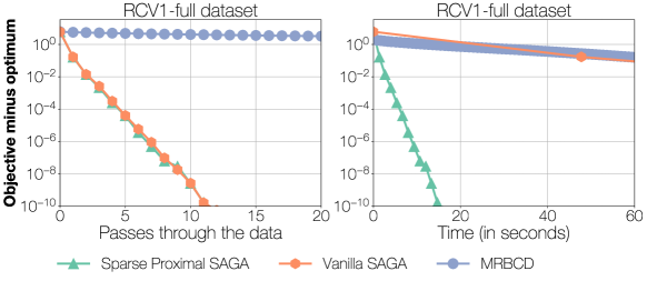
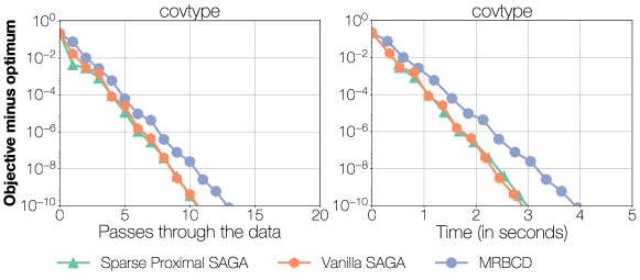
Figure 2: Suboptimality of different sequential algorithms. Each marker represents one pass through the dataset.

We observe that for the convergence behavior in terms of number of passes, Sparse Proximal Saga performs as well as vanilla Saga, though the latter requires dense updates at every iteration (Fig. 2 top left). On the other hand, in terms of running time, our implementation of Sparse Proximal Saga is much more efficient than the other methods for sparse input (Fig. 2 top right). In the case of dense input (Fig. 2 bottom), the three methods perform similarly.

A note on the performance of MRBCD.

It may appear surprising that Sparse Proximal Saga outperforms Mrbcd so dramatically on sparse datasets. However, one should note that Mrbcd is a doubly stochastic algorithm where both a random data point and a random coordinate are sampled for each iteration. If the data matrix is very sparse, then the probability that the sampled coordinate is in the support of the sampled data point becomes very low. This means that the gradient estimator term only contains the reference gradient term of Svrg, which only changes once per epoch. As a result, this estimator becomes very coarse and produces a slower empirical convergence.

This is reflected in the theoretical results given in Zhao et al. (2014), where the epoch size needed to get linear convergence are $k$ times bigger than the ones required by plain Svrg, where $k$ is the size of the set of blocks of coordinates.

Appendix F.2 Theoretical speedups.

In the experimental section, we have shown experimental speedup results where suboptimality was a function of the running time. This measure encompasses both theoretical algorithmic optimization properties and hardware overheads (such as contention of shared memory) which are not taken into account in our analysis.

In order to isolate these two effects, we now plot our speedup results in Figure 3 where suboptimality is a function of the number of iterations; thus, we abstract away any potential hardware overhead. To do so, we implement a global counter which is sparsely updated (every $100$ iterations for example) in order not to modify the asynchrony of the system. This counter is used only for plotting purposes and is not needed otherwise. Specifically, we define the theoretical speedup as:

$$\text{theoretical speedup}:=\text{(number of cores)}\,\frac{\text{number of iterations for sequential algorithm}}{\text{total number of iterations for parallel algorithm}}\,.$$

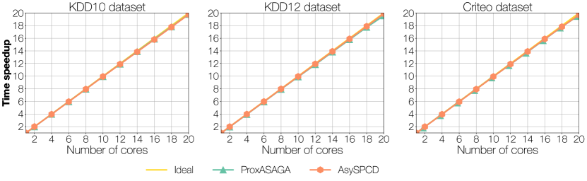
Figure 3: Theoretical optimization speedups for $\ell_{1}\!+\!\ell_{2}$-regularized logistic regression. Speedup as measured by the number of iterations required to reach $10^{-5}$ suboptimality for ProxAsaga and AsySpcd. In Fista the iterates are the same with different cores and so matches the “ideal” speedup.

We see clearly that the theoretical speedups obtained by both ProxAsagaand AsySpcd are linear (i.e. ideal). As we observe worse results in running time, this means that the hardware overheads of asynchronous methods are quite significant.

Appendix F.3 Timing benchmarks

We now provide the time it takes for the different methods with 10 cores to reach a suboptimality of $10^{-10}$. All results are in hours.

Dataset	ProxAsaga	AsySpcd	Fista
KDD 2010	1.01	13.3	5.2
KDD 2012	0.09	26.6	8.3
Criteo	0.14	33.3	6.6

Appendix F.4 Hyperparameters

The $\ell_{1}$-regularization parameter $\lambda_{2}$ was chosen as to give around 10% of non-zero features. The exact chosen values are the following: $\lambda_{2}=10^{-11}$ for KDD 2010, $\lambda_{2}=10^{-16}$ for KDD 2012 and $\lambda_{2}=4\times 10^{-12}$ for Criteo.

References

- Bauschke & Combettes (2011) Bauschke, Heinz and Combettes, Patrick L. Convex analysis and monotone operator theory in Hilbert spaces. Springer, 2011.
- Beck & Teboulle (2009) Beck, Amir and Teboulle, Marc. Gradient-based algorithms with applications to signal recovery. Convex Optimization in Signal Processing and Communications, 2009.
- Davis et al. (2016) Davis, Damek, Edmunds, Brent, and Udell, Madeleine. The sound of APALM clapping: faster nonsmooth nonconvex optimization with stochastic asynchronous PALM. In Advances in Neural Information Processing Systems 29, 2016.
- Defazio et al. (2014) Defazio, Aaron, Bach, Francis, and Lacoste-Julien, Simon. SAGA: A fast incremental gradient method with support for non-strongly convex composite objectives. In Advances in Neural Information Processing Systems, 2014.
- Gu et al. (2016) Gu, Bin, Huo, Zhouyuan, and Huang, Heng. Asynchronous stochastic block coordinate descent with variance reduction. arXiv preprint arXiv:1610.09447v3, 2016.
- Hsieh et al. (2015) Hsieh, Cho-Jui, Yu, Hsiang-Fu, and Dhillon, Inderjit S. PASSCoDe: parallel asynchronous stochastic dual coordinate descent. In ICML, 2015.
- Johnson & Zhang (2013) Johnson, Rie and Zhang, Tong. Accelerating stochastic gradient descent using predictive variance reduction. In Advances in Neural Information Processing Systems, 2013.
- Juan et al. (2016) Juan, Yuchin, Zhuang, Yong, Chin, Wei-Sheng, and Lin, Chih-Jen. Field-aware factorization machines for CTR prediction. In Proceedings of the 10th ACM Conference on Recommender Systems. ACM, 2016.
- Le Roux et al. (2012) Le Roux, Nicolas, Schmidt, Mark, and Bach, Francis R. A stochastic gradient method with an exponential convergence rate for finite training sets. In Advances in Neural Information Processing Systems, 2012.
- Leblond et al. (2017) Leblond, Rémi, Pedregosa, Fabian, and Lacoste-Julien, Simon. ASAGA: asynchronous parallel SAGA. Proceedings of the 20th International Conference on Artificial Intelligence and Statistics (AISTATS 2017), 2017.
- Liu & Wright (2015) Liu, Ji and Wright, Stephen J. Asynchronous stochastic coordinate descent: Parallelism and convergence properties. SIAM Journal on Optimization, 2015.
- Mania et al. (2017) Mania, Horia, Pan, Xinghao, Papailiopoulos, Dimitris, Recht, Benjamin, Ramchandran, Kannan, and Jordan, Michael I. Perturbed iterate analysis for asynchronous stochastic optimization. SIAM Journal on Optimization, 2017.
- Meng et al. (2017) Meng, Qi, Chen, Wei, Yu, Jingcheng, Wang, Taifeng, Ma, Zhi-Ming, and Liu, Tie-Yan. Asynchronous stochastic proximal optimization algorithms with variance reduction. In AAAI, 2017.
- Nesterov (2004) Nesterov, Yurii. Introductory lectures on convex optimization. Springer Science & Business Media, 2004.
- Nesterov (2013) Nesterov, Yurii. Gradient methods for minimizing composite functions. Mathematical Programming, 2013.
- Niu et al. (2011) Niu, Feng, Recht, Benjamin, Re, Christopher, and Wright, Stephen. Hogwild: A lock-free approach to parallelizing stochastic gradient descent. In Advances in Neural Information Processing Systems, 2011.
- Peng et al. (2016) Peng, Zhimin, Xu, Yangyang, Yan, Ming, and Yin, Wotao. ARock: an algorithmic framework for asynchronous parallel coordinate updates. SIAM Journal on Scientific Computing, 2016.
- Reddi et al. (2015) Reddi, Sashank J, Hefny, Ahmed, Sra, Suvrit, Poczos, Barnabas, and Smola, Alexander J. On variance reduction in stochastic gradient descent and its asynchronous variants. In Advances in Neural Information Processing Systems, 2015.
- Schmidt et al. (2016) Schmidt, Mark, Le Roux, Nicolas, and Bach, Francis. Minimizing finite sums with the stochastic average gradient. Mathematical Programming, 2016.
- Shalev-Shwartz & Zhang (2013) Shalev-Shwartz, Shai and Zhang, Tong. Stochastic dual coordinate ascent methods for regularized loss minimization. Journal of Machine Learning Research, 2013.
- Shalev-Shwartz et al. (2012) Shalev-Shwartz, Shai et al. Proximal stochastic dual coordinate ascent. arXiv preprint arXiv:1211.2717, 2012.
- Xiao & Zhang (2014) Xiao, Lin and Zhang, Tong. A proximal stochastic gradient method with progressive variance reduction. SIAM Journal on Optimization, 2014.
- You et al. (2016) You, Yang, Lian, Xiangru, Liu, Ji, Yu, Hsiang-Fu, Dhillon, Inderjit S, Demmel, James, and Hsieh, Cho-Jui. Asynchronous parallel greedy coordinate descent. In Advances In Neural Information Processing Systems, 2016.
- Yu et al. (2010) Yu, Hsiang-Fu, Lo, Hung-Yi, Hsieh, Hsun-Ping, Lou, Jing-Kai, McKenzie, Todd G, Chou, Jung-Wei, Chung, Po-Han, Ho, Chia-Hua, Chang, Chun-Fu, Wei, Yin-Hsuan, et al. Feature engineering and classifier ensemble for KDD cup 2010. In KDD Cup, 2010.
- Zhao et al. (2014) Zhao, Tuo, Yu, Mo, Wang, Yiming, Arora, Raman, and Liu, Han. Accelerated mini-batch randomized block coordinate descent method. In Advances in neural information processing systems, 2014.