Regular Potential Games

Abstract

A fundamental problem with the Nash equilibrium concept is the existence of certain “structurally deficient” equilibria that (i) lack fundamental robustness properties, and (ii) are difficult to analyze. The notion of a “regular” Nash equilibrium was introduced by Harsanyi. Such equilibria are isolated, highly robust, and relatively simple to analyze. A game is said to be regular if all equilibria in the game are regular. In this paper it is shown that almost all potential games are regular. That is, except for a closed subset with Lebesgue measure zero, all potential games are regular. As an immediate consequence of this, the paper also proves an oddness result for potential games: in almost all potential games, the number of Nash equilibrium strategies is finite and odd. Specialized results are given for weighted potential games, exact potential games, and games with identical payoffs. Applications of the results to game-theoretic learning are discussed.

1 Introduction

While the notion of Nash equilibrium (NE) is a universally accepted solution concept for games, several shortcomings have been noted over the years. A principal criticism (in addition to non-uniqueness) is that some Nash equilibrium strategies may be undesirable or unreasonable due to a lack of basic robustness properties. As a consequence, many equilibrium refinement concepts have been proposed [1, 2, 3, 4, 5, 6, 7], each attempting to single out subsets of Nash equilibrium strategies that satisfy some desirable criteria.

One of the most stringent refinement concepts, originally proposed by Harsanyi [3], is that a NE strategy be “regular.” In the words of van Damme [4], “regular Nash equilibria possess all the robustness properties that one can reasonably expect equilibria to possess.” Such equilibria are quasi-strict [3, 4], perfect [1], proper [2], strongly stable [6], essential [5], and isolated [4].

If all equilibria of a game are regular, then the number of NE strategies in the game has been shown to be finite and, curiously, odd [3, 8]. Regular equilibria have also been studied in the context of games of incomplete information, where, as part of Harsanyi’s celebrated purification theorem [9, 10, 11], they have been shown to be approachable.

A game is said to be regular if all equilibria in the game are regular. Harsanyi [3] showed that almost all games are regular, and hence, in almost all games, all equilibria possess all the robustness properties we might reasonably hope for.

While this result is a powerful when targeted at general $N$-player games, there are many important classes of games that have Lebesgue measure zero within the space of all games [12]. Harsanyi’s result tells us nothing about equilibrium properties within such special classes of games. This is the case, for example, in the important class of multi-agent games known as potential games [13].

A game is said to be a potential game if there exists some underlying function (generally referred to as the potential function) that all players implicitly seek to optimize. Potential games have many applications in economics and engineering [14, 13], and are particularly useful in the study of multi-agent systems, e.g., [15, 16, 17, 18, 19, 20, 21, 22, 23, 24, 25].

There are several types of potential games—in order of decreasing generality, these include weighted potential games, exact potential games, and games with identical payoffs [13, 26]. Letting WPG, EPG, and GIP denote the set of each of these types of potential games respectively, and letting G denote the set of all games, we have the following relationship:

$$\mbox{GIP}\subset\mbox{EPG}\subset\mbox{WPG}\subset\mbox{G},$$

where each subset is a low-dimensional (measure-zero) subset within any of its supersets. Harsanyi’s regularity result provides no information on the abundance (or dearth) of regular equilibria within these subclasses of games. Hence, when restricting attention to potential games, as is often done in the study of multi-agent systems, we are deprived of any generic results on the regularity, robustness, or finiteness of the equilibrium set.

We say that a property holds for almost all games in a given class if the subset of games in the class where the property fails to holds is a closed set with Lebesgue measure zero (with the dimension of the Lebesgue measure corresponding to the dimension of the given class of games—see Section 2.3 for more details).

The main result of this paper is the following theorem.

Theorem 1.

 
(i) Almost all weighted potential games are regular.
(ii) Almost all exact potential games are regular.
(iii) Almost all games with identical payoffs are regular.

We note that this result implies that for almost all games in each of these classes, all equilibria are quasi-strict, perfect, proper, strongly stable, essential, and isolated. Using Harsanyi’s oddness theorem (see [3], Theorem 1), we see that in any regular game, the number of NE strategies is finite and odd. Hence, the following result is an immediate consequence of Theorem 1.

Theorem 2.

In almost all weighted potential games, almost all exact potential games, and almost all games with identical payoffs, the number of NE strategies is finite and odd.

Regularity may be seen as serving two purposes. First, it ensures that the equilibrium set possesses the desirable structural properties noted above (e.g., equilibria are isolated, robust, and finite in number). Second, it simplifies the analysis of the game near equilibrium points—the important features of players’ utility functions near an equilibrium can be understood by looking only at first- and second-order terms in the associated Taylor series expansion. In this sense, the role of regular equilibria in games is analogous to the role that non-degenerate critical points play in the study of real-valued functions. This amenable analytic structure can greatly facilitate the study of (for example) game-theoretic learning processes [29, 30] or approachability in games with incomplete information [10].

As an application of these results to learning theory, in the paper [29] we consider the problem of studying continuous best-response dynamics (BR dynamics) [31, 32, 33] in potential games. BR dynamics are fundamental to learning theory—they model various forms of learning in games and underlie many popular game-theoretic learning algorithms including the canonical fictitious play (FP) algorithm [34]. While it is known that BR dynamics converge to the set of NE in potential games, the result is less than satisfactory. BR dynamics can converge to mixed-strategy (saddle-point) Nash equilibria and solutions of BR dynamics may be non-unique. Furthermore, little is understood about transient properties such as the rate of convergence of BR dynamics in potential games. (In fact, due to the non-uniqueness of solutions in potential games, it has been shown that it is impossible to establish convergence rate estimates for BR dynamics that hold at all points [35].)

In [29] we study how regular potential games can be used to address these issues. In particular, it is shown that in any regular potential game, BR dynamics converge generically to pure NE, solutions of BR dynamics are generically unique, and the rate of convergence of BR dynamics is generically exponential. Combined with the results of the present paper, this allows us to show that BR dynamics are “well behaved” in almost all potential games.

Furthermore, in [26] Monderer and Shapley study the convergence of the closely related FP algorithm in potential games and show convergence to the set of NE. In particular, they show that it is possible for FP to converge to completely mixed NE in potential games, which can be highly problematic for a number of reasons [36, 37, 29]. However, they conjecture that such behavior is exceptional; that is, they conjecture that in generic two-player potential games FP always converges to pure NE (see [26], Section 2). Regular potential games are well suited to studying this conjecture. Theorem 1 of the present paper combined with Theorem 1 of [29] shows that for the continuous-time version of FP [35, 39] (which is equivalent to BR dynamics after a time change [35]), this conjecture holds generically for potential games of arbitrary size; that is, in any regular potential game (and hence almost all potential games) continuous-time FP dynamics converge to pure NE from almost all initial conditions.

While regular equilibria have traditionally been studied as an equilibrium selection criterion in games, in potential games, pure strategy NE are naturally selected by virtue of the potential function. We emphasize that our objective in studying regular potential games is not to argue that (possibly mixed) regular equilibria are more natural than pure equilibria in potential games. Rather, we wish to demonstrate that (i) in almost all potential games, all equilibria possess desirable structural properties, (ii) properties that hold for regular potential games are inherently robust to payoff perturbations, and (iii) properties that hold only for irregular potential games are inherently nonrobust to payoff perturbations. We note, however, that our main result does imply that the two considerations (having a pure strategy regular NE) can be aligned in generic (i.e., regular) potential games where a potential maximizer must also be a regular equilibrium. We also remark that, as discussed earlier, regular potential games can be particularly useful in the study of game-theoretic learning processes, and a key aim of the present work is to facilitate the study of such learning processes by establishing the genericity of regular potential games.

The remainder of the paper is organized as follows. In Section 1.1 we outline our strategy for proving Theorem 1. Section 2 sets up notation. Section 3 presents a pair of key non-degeneracy conditions that are equivalent to regularity in potential games. Section 4 presents Proposition 13 which states that almost all identical payoff games are second-order non-degenerate (this proposition is the technical core of the paper) and sets up notation for analyzing second-order degeneracy (and regularity). Section 5 takes a brief digression to contrast proof techniques in general games vs potential games. Section 6 proves Proposition 13 . Section 7 proves that almost all identical payoff games are first-order non-degenerate. Section 8 proves that almost all exact and weighted potential games are regular. Section 9 concludes the paper.

1.1 Proof Strategy

Our strategy for proving Theorem 1 is as follows. A potential game will be seen to be regular if and only if the corresponding identical payoffs game (with the potential function being the common utility) is regular. Thus, the problem of proving Theorem 1 reduces, by and large, to the following proposition.

Proposition 3.

Almost all games with identical payoffs are regular.

The bulk of the paper will be devoted to proving this proposition. We will prove it as follows.

An equilibrium in an identical-payoffs (or potential) game can be shown to be regular if and only if the derivatives of the potential function satisfy two simple non-degeneracy conditions which we refer to as first- and second-order non-degeneracy (see Section 3). The first-order condition deals with the gradient of the potential function. (A first-order non-degenerate equilibrium is referred to as a quasi-strong equilibrium in [3], and a quasi-strict equilibrium in other works [4].) An equilibrium $x^{*}$ is second-order non-degenerate if the Hessian of the potential function taken with respect to the support of $x^{*}$ is invertible.

We say a potential game is first-order (second-order) non-degenerate if all equilibria in the game satisfy the first-order (second-order) non-degeneracy conditions. We will prove Proposition 3 by showing that:

1. An equilibrium of an identical payoffs game is regular if and only if it is first- and second order non-degenerate (see Section 3 Lemma 12),

2. Almost all games with identical payoffs are second-order non-degenerate (see Section 4.1 Proposition 13),

3. Almost all games with identical payoffs are first-order non-degenerate (see Section 7 Proposition 21).

We remark that in Propositions 13 and 21 we show that the subset of irregular games has (appropriately dimensioned) Lebesgue measure zero. By Remark 5 this is sufficient to establish regularity in almost all identical payoff games.

After proving Proposition 3, we extend the result to exact and weighted potential games. This extension is straightforward and is accomplished in Section 8 (see Proposition 22). Propositions 3 and 22 together prove Theorem 1.

2 Notation

We will outline the notation and terminology used throughout the paper below. A short glossary of additional standard notation used in the paper can be found in A.

2.1 Normal Form Games

A game in normal form is given by a tuple $\Gamma:=(N,(Y_{i},u_{i})_{i=1,\ldots,N}),$ where $N\in\{1,2,\ldots\}$ denotes the number of players, $Y_{i}:=\{y_{i}^{1},\ldots,y_{i}^{K_{i}}\}$ denotes the set of pure strategies (or actions) available to player $i$, with cardinality $K_{i}:=|Y_{i}|$, and $u_{i}:\prod_{j=1}^{N}Y_{j}\rightarrow\mathbb{R}$ denotes the utility function of player $i$.

Given some game $\Gamma$, let $Y:=\prod_{i=1}^{N}Y_{i}$ denote the set of joint pure strategies available to players, and let

$$K:=K_{1}\times\cdots\times K_{N}$$ (1)

denote the number of joint pure strategies. When defining spaces of games (e.g., as in Section 2.3) we will find it convenient to view $u_{i}=(u_{i}(y)_{y\in Y})$ as a vector in $\mathbb{R}^{K}$; we will clearly indicate when using this abuse of notation.

The set of mixed strategies of player $i$ is typically defined to be the probability simplex over $A_{i}$. It will simplify the presentation to consider an equivalent, but slightly modified, definition of the set of mixed strategies. Let

$$X_{i}:=\{x_{i}\in\mathbb{R}^{K_{i}-1}:~{}0\leq x_{i}^{k}\leq 1\mbox{ for }k=1,\ldots,K_{i}-1,\mbox{ and }\sum_{k=1}^{K_{i}-1}x_{i}^{k}\leq 1\},$$ (2)

denote the set of mixed strategies of player $i$. (This definition will allow us to perform calculations without being directly encumbered by the hyperplane constraint inherent in the probability simplex.) A strategy $x_{i}\in X_{i}$ is interpreted as follows: The scalar $1-\sum_{k=1}^{K_{i}}x_{i}^{k}$ represents the weight placed on the first pure strategy $y_{i}^{1}\in Y_{i}$, and for $k\in\{2,\ldots,K_{i}-1\}$, $x_{i}^{k-1}$ represents the weight placed on the $k$-th pure strategy $y_{i}^{k}$. In order to later reference this interpretation, the following notation will be useful. Given $x_{i}\in X_{i}$, let

$$T_{i}^{1}(x_{i}):=1-\sum_{k=1}^{K_{i}-1}x_{i}^{k}\quad\text{ and }\quad T_{i}^{k}(x_{i}):=x_{i}^{k-1},~{}~{}k\geq 2.$$ (3)

Let $X:=\prod_{i=1}^{N}X_{i}$ denote the set of joint mixed strategies and let $X_{-i}:=\prod_{j\not=i}X_{j}$. When convenient, given a mixed strategy $x=(x_{1},\ldots,x_{N})\in X$, we use the notation $x_{-i}$ to denote the tuple $(x_{j})_{j\not=i}$.

Given a mixed strategy $x\in X$, the expected utility of player $i$ is given by

$$U_{i}(x)=\sum_{k=1}^{K_{i}-1}x_{i}^{k}U_{i}(y_{i}^{k+1},x_{-i})+\left(1-\sum_{k=1}^{K_{i}-1}x_{i}^{k}\right)U_{i}(y_{i}^{1},x_{-i}).$$ (4)

A strategy $x\in X$ is said to be a Nash equilibrium (or simply an equilibrium) if $x_{i}\in\arg\max_{x_{i}^{\prime}\in X_{i}}U_{i}(x_{i}^{\prime},x_{-i})$ for all $x_{i}^{\prime}\in X_{i}$, $i=1,\ldots,N$.

We say that a strategy $x_{i}$ is completely mixed if it lies in the interior of $X_{i}$ and we say that $x_{i}$ is a pure strategy if is a vertex of $X_{i}$. Otherwise, we say that $x_{i}$ is an incompletely mixed strategy.

For $x_{i}\in X_{i}$, we define the carrier set of $x_{i}$ to be

$$\mbox{{carr}}_{i}(x_{i}):=\{y_{i}^{k}\in Y_{i}:T_{i}^{k}(x_{i})>0\},$$ (5)

that is, $\mbox{{carr}}_{i}(x_{i})$ is the subset of pure strategies in $Y_{i}$ that receive positive weight under $x_{i}$. (This is just a slight modification of the notion of a support set to the present context.) For $x=(x_{1},\ldots,x_{N})\in X$ let $\mbox{{carr}}(x):=\mbox{{carr}}_{1}(x_{1})\cup\cdots\cup\mbox{{carr}}_{N}(x_{N})$.

Suppose $C=C_{1}\cup\cdots\cup C_{N}$, where for each $i=1,\ldots,N$, $C_{i}$ is a nonempty subset of $Y_{i}$. We say that $C$ is the carrier for $x=(x_{1},\ldots,x_{N})\in X$ if $C=\mbox{{carr}}(x)$, or equivalently, if $C_{i}=\mbox{{carr}}_{i}(x_{i})$ for $i=1,\ldots,N$.

2.2 Potential Games

Following [13, 26], a game is said to be a weighted potential game if there exists a function $u:Y\rightarrow\mathbb{R}$ and a vector of positive weights $(w_{i})_{i=1}^{N}\in\mathbb{R}^{N}$ such that

$$u_{i}(y_{i}^{\prime},y_{-i})-u_{i}(y_{i}^{\prime\prime},y_{-i})=w_{i}\big{(}u(y_{i}^{\prime},y_{-i})-u(y_{i}^{\prime\prime},y_{-i})\big{)}$$ (6)

A game is said to be an exact potential game if (6) holds with $w_{i}=1$ for all $i=1,\ldots,N$. A game is said to be an identical-payoffs game if there exists a function $u:Y\rightarrow\mathbb{R}$ such that $u_{i}(y)=u(y)$ for all $y\in Y$, $i=1,\ldots,N$.

When we refer simply to a “potential game” we mean a weighted potential game, which includes the other classes of games as special cases.

Given a potential game, we let $U:X\to\mathbb{R}$ be the multilinear extension of $u$ defined by

$$U(x)=\sum_{k=1}^{K_{i}-1}x_{i}^{k}U(y_{i}^{k+1},x_{-i})+\left(1-\sum_{k=1}^{K_{i}-1}x_{i}^{k}\right)U(y_{i}^{1},x_{-i}).$$ (7)

We will typically refer to $U$ as the potential function and to $u$ as the pure form of the potential function.

By way of notation, given a pure strategy $y_{i}\in Y_{i}$ and a mixed strategy $x_{-i}\in X_{-i}$, we will write $U(y_{i},x_{-i})$ to indicate the value of $U$ when player $i$ uses a mixed strategy placing all weight on the $y_{i}$ and the remaining players use the strategy $x_{-i}\in X_{-i}$.

2.3 Almost All Games

The following definition specifies the notion of “almost all” to be used in the paper.

Definition 4.

Given some property $\mathcal{S}$, we say that $\mathcal{S}$ holds for almost all points in some Euclidean space $\mathbb{R}^{n}$ if the set where $\mathcal{S}$ fails to hold is a closed set with $\mathcal{L}^{n}$-measure zero.

We say that a game $\Gamma$ has size $(N,(K_{i})_{i=1}^{N})$ if $\Gamma$ is a general $N$-player game and the size of the action space of each player satisfies $|Y_{i}|=K_{i}\in\{2,3,\ldots\}$, $i=1,\ldots,N$. Let $K$ be as defined in (1) so that $K$ gives the number of pure strategies in a game of size $(N,(K_{i})_{i=1}^{N})$.

A game of size $(N,(K_{i})_{i=1}^{N})$ is uniquely represented by the vector $u:=(u_{i}(y))_{y\in Y,~{}i=1,\ldots,N}\in\mathbb{R}^{NK}$ which specifies the utility received by each player for each pure strategy $y\in Y$. We will frequently refer to $u$ as the vector of utility coefficients. The set of all games of this size is equivalent to $\mathbb{R}^{NK}$.

Let $\mathcal{W},\mathcal{P},\mathcal{I}\subset\mathbb{R}^{NK}$, denote the subsets of weighted potential games, exact potential games, and identical-payoffs games respectively. (An explicit construction of $\mathcal{W}$ and $\mathcal{P}$ can be found in Section 8.) Let $K_{w}:=\dim\mathcal{W}$ and $K_{p}:=\dim\mathcal{P}$. The sets of weighted and exact potential games are equivalent to the Euclidean spaces $\mathbb{R}^{K_{w}}$ and $\mathbb{R}^{K_{p}}$ respectively.

An identical-payoffs game is uniquely represented as a vector $u\in\mathbb{R}^{K}$ denoting the payoff (identical for all players) received for each action $y\in Y$, and we will represent this set of games as $\mathcal{I}:=\mathbb{R}^{K}.$

For a fixed game size, each class of games discussed above is equivalent to some Euclidean space. We will say that almost all games in a given class are regular if, for any game size, almost all games (per Definition 4) in the class are regular.

Remark 5 (Closedness).

It was shown by Harsanyi [3, 4] that the set of irregular games of (any) size $(N,(K_{i})_{i=1}^{N})$ is a closed subset in the space of all games of size $(N,(K_{i})_{i=1}^{N})$. It is straightforward to extend this result to the various subclasses of potential games. In particular, we have:
(i) The set of irregular weighted potential games is closed with respect to $\mathcal{W}$.
(ii) The set of irregular exact potential games is closed with respect to $\mathcal{P}$.
(iii) The set of irregular games with identical payoffs is closed with respect to $\mathcal{I}$.

For practical purposes this means that in order to verify that almost all potential games of a given class are regular, we need only verify that the subset of irregular games has appropriately dimensioned Lebesgue measure zero.

3 Regular Equilibria in Potential Games

In potential games, regular equilibria have a simple and intuitive meaning. An equilibrium in a potential game is regular if (i) it is quasi-strict in the sense of [4] (a condition we will refer to as first-order non-degeneracy), and (ii) the Hessian of $U$ (the potential) taken with respect to the support of the equilibrium is invertible (a condition we will refer to as second order non-degeneracy). For equilibria in the interior of the strategy space, this simply reduces to an equilibrium being regular if and only if it is a non-degenerate critical point of $U$ in the traditional sense.

Since the non-degeneracy conditions given in this section (applicable only within the class of potential games) are simpler to work with than the traditional definition of regularity, we will work with directly with these conditions through the remainder of the paper. However, the traditional definition of regularity can be found in Section 5 (see Definition 14) where we contrast our techniques with those required in general games.

The remainder of the section is organized as follows. In Sections 3.1–3.2 we define the notions of first and second-order degeneracy. In Section 3.3 we show that, in a potential game, these conditions are equivalent to regularity.

3.1 First-Order Degeneracy

Let $C=C_{1}\cup\cdots\cup C_{N}$, $C_{i}\subset Y_{i}$ $\forall i=1,\ldots,N$ be some carrier set. Let $\gamma_{i}:=|C_{i}|$ and assume that the strategy set $Y_{i}$ is reordered so that $\{y_{i}^{1},\ldots,y_{i}^{\gamma_{i}}\}=C_{i}$. Under this ordering, the first $\gamma_{i}-1$ components of any strategy $x_{i}$ with $\mbox{{carr}}_{i}(x_{i})=C_{i}$ are free (not constrained to zero by $C_{i}$) and the remaining components of $x_{i}$ are constrained to zero. That is, the subvector $(x_{i}^{k})_{k=1}^{\gamma_{i}-1}$ is free under $C_{i}$ and the subvector $(x_{i}^{k})_{k=\gamma_{i}}^{K_{i}}=0$. The set of strategies $\{x\in X:~{}\mbox{{carr}}(x)=C\}$ is precisely the interior of the face of $X$ given by

$$X_{C}:=\{x\in X:~{}x_{i}^{k}=0,~{}k=\gamma_{i},\ldots,K_{i}-1,~{}i=1,\ldots,N\}.$$ (8)

Definition 6 (First-Order Degenerate Equilibrium).

Suppose $\Gamma$ is a potential game with potential function $U$. Suppose $x^{*}\in X$ is an equilibrium of $\Gamma$ with carrier $C$. We say that $x^{*}$ is a first-order degenerate equilibrium if there exists a pair $(i,k)$, $i=1,\ldots,N$, $k=\gamma_{i},\ldots,K_{i}-1$ such that

$$\frac{\partial U(x^{*})}{\partial x_{i}^{k}}=0$$ (9)

and we say $x^{*}$ is first-order non-degenerate otherwise.

We note that the condition (9) in the definition of first-order degeneracy is implicitly dependent on the carrier $C$ (since $\gamma_{i}=|C_{i}|$ and we assume that $C_{i}=\{y_{i}^{1},\ldots,y_{i}^{\gamma_{i}}\}$).

Definition 7 (First-order Degenerate Game).

We say a game is first-order degenerate if it has an equilibrium that is first-order degenerate, and we say the game is first-order non-degenerate otherwise.

Example 8.

Consider the $3\times 2$ identical-payoffs game with payoff matrices

$$M_{1}=\begin{pmatrix}1&-4\\ -1&1\end{pmatrix}\quad M_{2}=\begin{pmatrix}-1&1\\ 1&2\end{pmatrix},$$

where player 1 is the “row player”, player 2 is the “column player”, and player 3 is the “matrix player.” Recalling that $x_{i}$ denotes the probability of player $i$ playing action $y_{i}^{2}$ (since each player has only two strategies, we drop the superscipts on $x_{i}$), this game has a first-order degenerate equilibrium at the strategy $x^{*}=(1/2,0,1/2)$.

This may be visualized in terms of the gradient of $U$. The three (gradient) level surfaces along which $\frac{\partial U(x)}{\partial x_{i}}=0$, $i=1,2,3$, are displayed in Figures 1(a)–1(b). The equilibrium $x^{*}$ has carrier $C=Y_{1}\cup\{y_{2}^{1}\}\cup Y_{3}$ and lies on the face of $X$ given by $\{x\in X:x_{2}=0\}$. Yet, $x^{*}$ also lies at the intersection of all three level surfaces (and thus is a bona fide critical point of $U$). In particular, $x^{*}$ lies on the level surface, $\{x:\frac{\partial U(x^{*})}{\partial x_{2}}=0\}$, making it first-order degenerate.

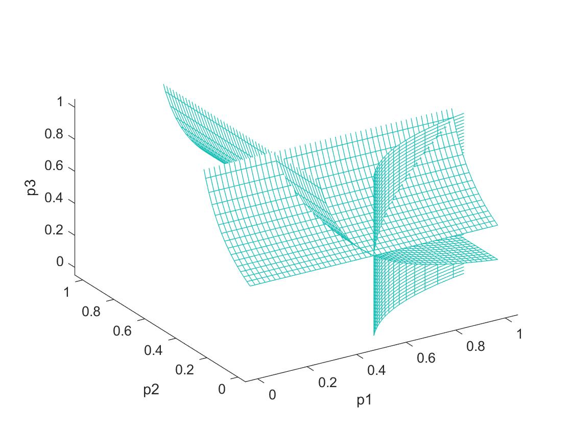
(a) Level surfaces of $\frac{\partial U(x)}{\partial x_{i}}$, $i=1,2,3$.

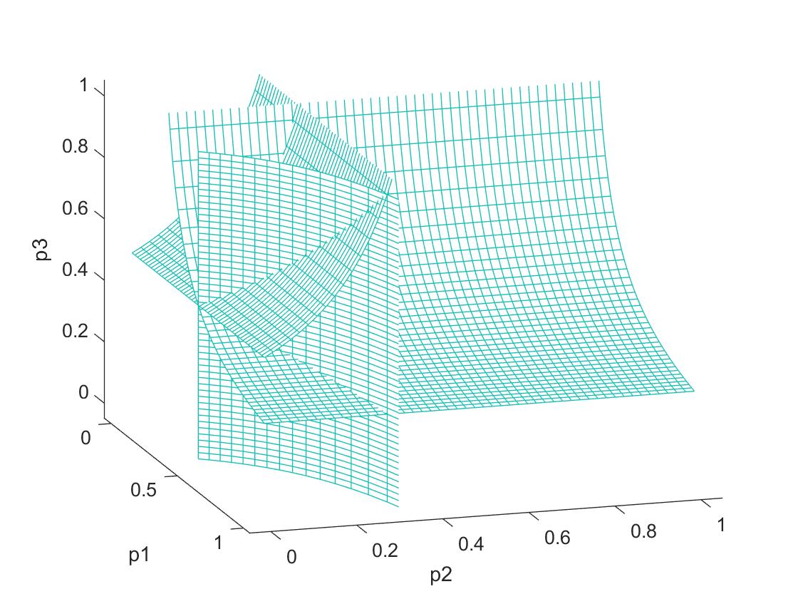
(b) Alternate view of gradient level surfaces.

Remark 9 (Equivalence to Quasi-Strict Equilibria).

An equilibrium $x^{*}$ with carrier $C$ is first order non-degenerate if and only if, for every player $i$, the set of pure-strategy best responses to $x_{-i}^{*}$ coincides with $C_{i}$. (This is verified using the multi-linearity of $U$.) We note that, using this later definition, Harsanyi [3] referred to first-order non-degenerate equilibria as quasi-strong equilibria. In other works these have been referred to as quasi-strict equilibria [4]. We prefer to use the term first-order non-degenerate in order to emphasize that we are concerned with the gradient of the potential function and to keep the nomenclature consistent with the notion of second-order non-degeneracy, introduced next.

3.2 Second-Order Degeneracy

Suppose that $\Gamma$ is a potential game with potential function $U$. Let $C$ be some carrier set. Let $\tilde{N}:=|\{i=1,\ldots,N:~{}\gamma_{i}\geq 2\}|$, and assume that the player set is ordered so that $\gamma_{i}\geq 2$ for $i=1,\ldots,\tilde{N}$. Under this ordering, for strategies with $\mbox{{carr}}(x)=C$, the first $\tilde{N}$ players use mixed strategies and the remaining players use pure strategies. Assume that $\tilde{N}\geq 1$ so that any $x$ with carrier $C$ is a genuine mixed (not pure) strategy.

Let the Hessian of $U$ taken with respect to $C$ be given by

$$\tilde{{\bf H}}(x):=\left(\frac{\partial^{2}U(x)}{\partial x_{i}^{k}\partial x_{j}^{\ell}}\right)_{\begin{subarray}{c}i,j=1,\ldots,\tilde{N},\\ k=1,\ldots,\gamma_{i}-1,\\ \ell=1,\ldots,\gamma_{j}-1\end{subarray}}.$$ (10)

Note that this definition of the Hessian restricts attention to the components of $x$ that are free (i.e., unconstrained) under $C$. That is, $\tilde{\bf H}(x)$ taken with respect to $C$ is the Hessian of $U|_{X_{C}}$ at $x$.

Definition 10 (Second-Order Degenerate Equilibrium).

Let $\Gamma$ be a potential game with potential function $U$. We say an equilibrium $x^{*}\in X$ of $\Gamma$ is second-order degenerate if the Hessian $\tilde{{\bf H}}(x^{*})$ taken with respect to $\mbox{{carr}}(x^{*})$ is singular, and we say $x^{*}$ is second-order non-degenerate otherwise.

Definition 11 (Second-Order Degenerate Game).

We say a game is second-order degenerate if it has an equilibrium that is second-order degenerate, and we say the game is second-order non-degenerate otherwise.

3.3 Regular Equilibria and Non-Degeneracy Conditions

The following lemma shows that within the class of potential games, the first and second-order non-degeneracy conditions defined above are equivalent to regularity.

Lemma 12.

Let $\Gamma$ be a potential game. Then,
(i) If an equilibrium $x^{*}$ is first-order non-degenerate, then it is second-order non-degenerate if and only if it is regular.
(ii) If an equilibrium $x^{*}$ is regular, then it is first-order non-degenerate.

In particular, an equilibrium $x^{*}$ is regular if and only if it is both first and second-order non-degenerate.

The proof of this lemma follows readily from the definitions of regularity (see Definition 14) and first and second-order degeneracy, and is omitted for brevity.

4 Second-Order Degeneracy in Games with Identical Payoffs

In the previous section we established that a game is regular if and only if it is first- and second-order non-degenerate. In this section we will state our main result regarding second-order non-degeneracy—namely, that the set of identical payoff games that are second-order degenerate has Lebesgue measure zero (see Proposition 13). Later, in Section 7 we will show the analogous result for first-order degenerate games (Proposition 21). By Remark 5, this will be sufficient to prove Proposition 3.

This section is organized as follows. In Section 4.1 we state our main result for second-order degenerate games. In Section 4.2 we outline our strategy for proving Proposition 13. In Section 4.3 we set up notation required for the analysis of second-order non-degeneracy (and the traditional notion of regularity). The proof of Proposition 13 will then be given in Section 6 after a brief interlude to discuss general games.

4.1 Second-Order Degenerate Games

In the following proposition we will assume the number of players $N$ and action-space sizes $K_{i}$, $i=1,\ldots,N$ are fixed, and let $K$ be as defined in (1).

Proposition 13.

The set of identical-payoff games that are second-order degenerate has $\mathcal{L}^{K}$-measure zero.

This proposition will be proved in Section 4.3.

4.2 Roadmap of Proof of Proposition 13

Our strategy for proving Proposition 17 will be as follows.

1. Fix a carrier set $C$ with $|C|=\gamma$. Following (8), let

$$X^{*}_{C}:=\{x:\mbox{{carr}}(x)=C\}.$$

We will begin by deducing that for any equilibrium $x^{*}\in X^{*}_{C}$, the key relation (21) holds, where ${\bf A}(x)$ is defined in (20).

2. Proposition 17 shows that for every $x\in X^{*}_{C}$, the matrix ${\bf A}(x)$ has full row rank.

3. Using Proposition 17 we construct a countable cover $(B_{\ell})_{\ell\geq 1}$ of $X^{*}_{C}$ such that for each $\ell$, we may choose $\gamma$ columns of ${\bf A}(x)\in\mathbb{R}^{\gamma\times K}$ so that these same columns are linearly independent for all $x\in B_{\ell}$. For each $\ell$, the associated columns form an invertible square submatrix of ${\bf A}(x)$ for all $x\in B_{\ell}$. Using this invertible submatrix and (21), we construct a mapping $\rho_{\ell}:B_{\ell}\times\mathbb{R}^{K-\gamma}\to\mathbb{R}^{K}$, which allows us to recover the full vector of potential coefficients $u\in\mathbb{R}^{K}$ given an equilibrium $x^{*}\in X^{*}_{C}$ and a $(K-\gamma)$-dimensional subvector of the potential coefficients. (See Lemma 18, (31)–(32), and Corollary 19.)

4. We then demonstrate that if $x^{*}\in B_{\ell}$ is a NE of a game with potential-function coefficients $u\in\mathbb{R}^{K}$, then $x^{*}$ is second-order degenerate if and only if the Jacobian of $\rho_{\ell}$ is non-invertible. (See Lemma 20.) Since the output of $\rho_{\ell}$ is the full vector of coefficients $u$, this implies that $u$ lies in the set of critical values of $\rho_{\ell}$ (i.e. the set of outputs of $\rho_{\ell}$ at which the Jacobian is not invertible).

5. From here, the proof follows from Sard’s theorem [41]. In particular, applying Sard’s theorem to $\rho_{\ell}$ shows that the set of games with second-order degenerate equilibria lying in $B_{\ell}$ has measure zero. Repeating this argument over all $B_{\ell}$ (of which there is a countable number) and for all carriers $C$ (of which there is a finite number) yields Proposition 13.

We remark that the above proof strategy follows the same general strategy used by Harsanyi in [3] to prove regularity in general games. However, important technical challenges arise in the case of potential games that are not present in general games. This is discussed further in Sections 5.2–5.3.

4.3 Analysis of Second-Order Degeneracy: Setup

Proposition 13 will be proved using Sard’s theorem as outlined above. In this section we introduce some pertinent notation that will allow us to establish (21), which is the key relationship allowing us to analyze second-order degeneracy.

Note that the set of joint pure strategies $Y$ may be expressed as an ordered set $Y=\{y^{1},\ldots,y^{K}\}$ where each $y^{\tau}\in Y$, is an $N$-tuple of strategies, $\tau\in\{1,\ldots,K\}$. We will assume a particular ordering for this set after Proposition 17.

In an identical-payoffs game there exists a single function $u:Y\to\mathbb{R}$ such that $u_{i}=u$ for all $i=1,\ldots,N$. If we consider the vector of utility coefficients $u=(u(y))_{y\in Y}\in R^{K}$ as a variable, then by (7), $U$ is linear in $u$. At this point we will express $U$ in a more convenient form (see (12)) which more clearly exposes this relationship.

Let $\tau\in\{1,\ldots,K\}$, $i\in\{1,\ldots,N\}$ and $x_{i}\in X_{i}$. We define $q_{i}^{\tau}:X_{i}\rightarrow[0,1]$ by

$$q^{\tau}_{i}(x_{i}):=T_{i}^{k}(x_{i})$$ (11)

where $k$ corresponds to the action played by player $i$ in the tuple $y^{\tau}$, i.e, $(y^{\tau})_{i}=y_{i}^{k}$, and where $T_{i}^{k}(x_{i})$ is defined in (3). In words, given some mixed strategy $x_{i}\in X_{i}$, $q_{i}^{\tau}(x_{i})$ gives the weight $x_{i}$ places on the particular action used by player $i$ in the $\tau$-th action tuple $y^{\tau}$.

In an abuse of notation, given a pure strategy $y_{i}^{k}\in Y_{i}$, we let $q_{i}^{\tau}(y_{i}^{k})=1$ if $(y^{\tau})_{i}=y_{i}^{k}$ and $q_{i}^{\tau}(y_{i}^{k})=0$ otherwise.

Given a fixed vector of utility coefficients $u\in\mathbb{R}^{K}$, the utility function $U:X\rightarrow\mathbb{R}$ may be expressed as

$$U(x)=\sum_{\tau=1}^{K}u^{\tau}\left[\prod_{i=1}^{N}q_{i}^{\tau}(x_{i})\right].$$ (12)

Note that this form makes it clear that $U$ is linear in $u$.

Now, let $C=C_{1}\cup\cdots\cup C_{N}$ be some carrier set. The analysis through the remainder of the section will rely on this carrier set being fixed, and many of the subsequent terms are implicitly dependent on the choice of $C$. In keeping with our prior convention we let $\gamma_{i}:=|C_{i}|$, and let $\tilde{N}:=|\{i\in\{1,\ldots,N\}:\gamma_{i}\geq 2\}|$, and without loss of generality we assume that the strategies in $Y_{i}$ are ordered so that $C_{i}=\{y_{i}^{1},\ldots,y_{i}^{\gamma_{i}}\}$.

Any $x_{i}$ with carrier $C_{i}$ has precisely $\gamma_{i}-1$ free components (i.e., not constrained to zero by $C_{i}$). The joint strategy $x=(x_{1},\ldots,x_{N})$ is a vector with

$$\gamma:=\sum_{i=1}^{N}(\gamma_{i}-1)$$ (13)

free components.

By (7) we have that

$$\frac{\partial U(x)}{\partial x_{i}^{k}}=U(y_{i}^{k+1},x_{-i})-U(y_{i}^{1},x_{-i})=:F_{i}^{k}(x,u)$$ (14)

for $i=1,\ldots,\tilde{N},~{}k=1,\ldots,\gamma_{i}-1$. Let

$$F(x,u):=\left(F_{i}^{k}(x,u)\right)_{\begin{subarray}{c}i=1,\ldots,\tilde{N}\\ k=1,\ldots,\gamma_{i}-1\end{subarray}}.$$ (15)

Given an $x\in X$, it is at times useful to decompose it as $x=(x_{p},x_{m})$, where $x_{m}=(x_{i}^{k})_{i=1,\ldots,\tilde{N},~{}k=1,\ldots,\gamma_{i}-1}$ and $x_{p}$ contains the remaining components of $x$. (The subscript of $x_{m}$ is indicative of “mixed strategy components” of $x$ and $x_{p}$ indicative of “pure strategy components” of $x$.) In this decomposition, $x_{m}$ is a $\gamma$-dimensional vector containing the free components of $x$. Taking the Jacobian of $F$ in terms of the components of $x_{m}$ we find that

$$D_{x_{m}}F(x_{p},x_{m},u)=\tilde{{\bf H}}(x),$$ (16)

where $D_{x_{m}}F(x_{p},x_{m},u)=\left(\frac{\partial F}{\partial x_{i}^{\ell}}\right)_{\begin{subarray}{c}i=1,\ldots,{\tilde{N}},\\ \ell=1,\ldots,\gamma_{i}-1\end{subarray}}$.

Let $x^{*}$ be a mixed equilibrium with carrier $C$. Differentiating (7) we see that at the equilibrium $x^{*}$ we have $\frac{\partial U(x^{*})}{\partial x_{i}^{k}}=0$, or equivalently,

$$F_{i}^{k}(x^{*},u)=U(y_{i}^{k+1},x^{*}_{-i})-U(y_{i}^{1},x^{*}_{-i})=0$$ (17)

for $i=1,\ldots,\tilde{N},~{}k=1,\ldots,\gamma_{i}-1$. Using (12) in the above we get

$$F_{i}^{k}(x^{*},u)=\sum_{\tau=1}^{K}u^{\tau}\left[\left(q^{\tau}_{i}(y_{i}^{k+1})-q^{\tau}_{i}(y_{i}^{1})\right)\prod_{j\not=i}q^{\tau}_{j}(x^{*}_{j})\right]=0.$$ (18)

Note that (18) is a linear in $u$. We would like to express (18) as a matrix equation (i.e., ${\bf A}(x)u=0$ for some matrix ${\bf A}(x)$ dependent only on $x$). With this in mind, it will be convenient to develop notation relating the ordering of the pure-strategy set $Y$ with the ordering of $(F_{i}^{k})_{i=1,\ldots,\tilde{N},~{}k=1,\ldots,\gamma_{i}-1}$. Given $i\in\{1,\ldots,\tilde{N}\}$, $k\in\{1,\ldots,\gamma_{i}-1\}$, let

$$s^{*}(i,k):=\begin{cases}k&\mbox{ for }~{}i=1,\\ \sum_{j=1}^{i-1}(\gamma_{j}-1)+k&\mbox{ for }~{}i\geq 2.\end{cases}$$

Define $i^{*}:\{1,\ldots,\gamma\}\to\{1,\ldots,\tilde{N}\}$ and $k^{*}:\{1,\ldots,\gamma\}\to\{1,\ldots,\max_{i}\{\gamma_{i}-1\}\}$ to be the inverse of $s^{*}$; that is

$$s^{*}(i^{*}(s),k^{*}(s))=s$$ (19)

for all $s=1,\ldots,\gamma$.

The above notation may be understood as follows: Effectively, we have stacked $(F_{i}^{k})_{i=1,\ldots,\tilde{N},~{}k=1,\ldots,\gamma_{i}-1}$ into a single vector. Given a pair $(i,k)$, the function $s(i,k)\in\{1,\ldots,\gamma\}$ gives the corresponding index in this vector. Conversely, given some $s\in\{1,\ldots,\gamma\}$, the functions $i^{*}(s)$ and $k^{*}(s)$ simply return the player $i$ or action $k$ corresponding to entry $s$ in the vector.

Given an $x\in X$, let ${\bf A}(x)=\left(a_{s,\tau}(x)\right)_{\begin{subarray}{c}s=1,\ldots,\gamma,\\ \tau=1,\ldots,K\end{subarray}}\in\mathbb{R}^{\gamma\times K}$ be defined as the matrix with entries

$$a_{s,\tau}(x):=\left(q^{\tau}_{i^{*}(s)}(y_{i}^{k^{*}(s)+1})-q^{\tau}_{i^{*}(s)}(y_{i}^{1})\right)\prod_{j\not=i^{*}(s)}q^{\tau}_{j}(x_{j}),$$ (20)

Reexpressing (18) using this notation, we see that for any equilibrium $x^{*}$ with carrier $C$ we have

$${\bf A}(x^{*})u=0.$$ (21)

5 General Games: Discussion and Proof Techniques

In this section we take a short digression to discuss the proof that almost all general games are regular, and contrast this with the potential games case. We note that this section may be skipped without loss of continuity.

In Section 5.1 we recall the traditional definition of a regular equilibrium. In Section 5.2 we discuss the strategy used by Harsanyi [3] to prove that almost all general games are regular. In Section 5.3 we discuss the technical challenges arising in the case of potential games and contrast our proof techniques with those used by Harsanyi.

5.1 Regular Equilibria in General Games

We now recall the traditional definition a regular equilibrium as given in [40, 4]. Let the game size $(N,(K_{i})_{i=1}^{N})$ be fixed.

As discussed in Section 2.3, a game is uniquely defined by a vector $u\in\mathbb{R}^{NK}$ (which we refer to as the utility coefficient vector) specifying the pure-strategy utility received by each player.

Given a strategy $x\in X$ and vector of utility coefficients $u\in\mathbb{R}^{NK}$, let

$$\tilde{F}_{i}^{k}(x,u) :=T_{i}^{1}(x_{i})x_{i}^{k}[U_{i}(y_{i}^{k+1},x_{-i})-U_{i}(y_{i}^{1},x_{-i})]$$ (22)

for $i=1,\ldots,N$, $k=1,\ldots,K_{i}-1$, and let

$$\tilde{F}(x,u):=\left(\tilde{F}_{i}^{k}(x,u)\right)_{\begin{subarray}{c}i=1,\ldots,N\\ k=1,\ldots,K_{i}-1\end{subarray}}.$$ (23)

Definition 14 (Regular Equilibrium).

Let $x^{*}\in X$ be an equilibrium of a game with utility coefficient vector $u$. Assume the action set $Y_{i}$ of each player is reordered so that $y_{i}^{1}\in\mbox{{carr}}_{i}(x_{i}^{*})$. The equilibrium $x^{*}$ is said to be regular if the Jacobian of $\tilde{F}(x^{*},u)$, given by $D_{x}\tilde{F}(x^{*},u)$, is non-singular.

Remark 15.

We note that if $x^{*}$ is regular, then the Jacobian of $\tilde{F}(x^{*},u)$ can be shown to be nonsingular under any reordering of $Y_{i}$ in which the reference action satisfies $y_{i}^{1}\in\mbox{{carr}}_{i}(x_{i}^{*})$ for all $i=1,\ldots,N$ (see [40], Theorem 3.8). This justifies the use of an arbitrary reference action $y_{i}^{1}\in\mbox{{carr}}_{i}(x_{i}^{*})$ in the above definition.

Remark 16.

The notion of a regular equilibrium is traditionally defined by considering mixed strategies directly in the probability simplex rather than $X_{i}$ [4]. Using the definition of $\tilde{F}_{i}^{k}$ and the properties of the determinant of a matrix, it is readily confirmed that the definition of regularity given in Definition 14 coincides with the traditional definition in [4].

5.2 Almost All General Games are Regular: Proof Strategy

We will now review, at a high level, the classical technique for proving that almost all general games are regular given in [3].

The strategy is as follows.

1. Suppose that a carrier set $C$ is fixed.

2. Let $u\in\mathbb{R}^{NK}$ denote a vector of utility function coefficients, and let $u$ be broken down as $u=(u^{*},u^{**})$, where $u^{*}\in\mathbb{R}^{\gamma}$, $u^{**}\in\mathbb{R}^{NK-\gamma}$.

3. Construct a $C^{1}$ function $\rho^{**}:X^{*}_{C}\times\mathbb{R}^{NK-\gamma}\to\mathbb{R}^{\gamma}$ such that, given any equilibrium $x^{*}$ with carrier $C$ and a partial vector of utility coefficients $u^{**}\in\mathbb{R}^{NK-\gamma}$, we have

   $$u^{*}=\rho^{**}(x^{*},u^{**}).$$

   That is, $\rho^{**}$ allows one to recover $u^{*}$ given $x^{*}$ and $u^{**}$. Given $\rho^{**}$, it is trivial to construct a $C^{1}$ function $\rho^{*}:X^{*}_{C}\times\mathbb{R}^{NK-\gamma}\to\mathbb{R}^{NK}$ such that

   $$u=\rho^{*}(x^{*},u^{**}),$$

   so that $\rho^{*}$ recovers the full vector $u$ given $x^{*}$ and $u^{**}$.

4. Show that the set of all irregular games having an equilibrium with carrier $C$ lies in the “critical values” set of $\rho^{*}$ (i.e, the image of the set of critical points). By Sard’s theorem, this implies that all such games lie in an $\mathcal{L}^{NK}$-measure zero set.

5. Since the argument holds for arbitrary carrier $C$ and there are a finite number of possible carriers, this completes the proof.

The crucial task in the above proof outline is the construction of the function $\rho^{**}$ which isolates the set of irregular games in a critical values set. For the sake of comparison with the identical payoff games case, we will now review the technique for constructing $\rho^{**}$ in [3] more detail.

Suppose a carrier $C$ is fixed, and suppose $x^{*}$ is an equilibrium with carrier $C$. Differentiating (using the same reasoning used to arrive at (17)) we see that at $x^{*}$ we have

$$U_{i}(y_{i}^{k+1},x_{-i}^{*})-U_{i}(y_{i}^{1},x_{-i}^{*})=0$$ (24)

for $i=1,\ldots,\tilde{N}$, $k=1,\ldots,\gamma_{i}-1$. Let $u=(u_{1},\ldots,u_{N})\in\mathbb{R}^{NK}$ represent the vector of all player’s pure-strategy utilities. As with (17), the equality (24) is linear in $u$ and may be expressed as a matrix equation

$${\bf B}(x)u=0,$$ (25)

where ${\bf B}(x)\in\mathbb{R}^{\gamma\times NK}$. The matrix ${\bf B}(x)$ has particularly convenient structure. To elucidate this structure, first note that, as with (12), the (expected) utility of player $i$ in a general game may be expressed as

$$U_{i}(x)=\sum_{\tau=1}^{K}u_{i}^{\tau}\left[\prod_{i=1}^{N}q_{i}^{\tau}(x_{i})\right].$$

Using this form, the equality (24) is expressed as

$$\sum_{\tau=1}^{K}u_{i}^{\tau}\left[\left(q^{\tau}_{i}(y_{i}^{k+1})-q^{\tau}_{i}(y_{i}^{1})\right)\prod_{j\not=i}q^{\tau}_{j}(x^{*}_{j})\right]=0,$$ (26)

for $i=1,\ldots,\tilde{N}$, $k=1,\ldots,\gamma_{i}-1$. For each $i\in\{1,\ldots,\tilde{N}\}$, let ${\bf B}_{i}(x)=(b_{i,k,\tau}(x))_{\begin{subarray}{c}k=1,\ldots,\gamma_{i}-1\\ \tau=1,\ldots,K\end{subarray}}$ be the matrix with entries

$$b_{i,k,\tau}(x):=\left(q^{\tau}_{i}(y_{i}^{k+1})-q^{\tau}_{i}(y_{i}^{1})\right)\prod_{j\not=i}q^{\tau}_{j}(x_{j}).$$ (27)

The equality (26) may now be expressed in the form of (25) with ${\bf B}(x)$ given by

$${\bf B}(x):=\begin{pmatrix}{\bf B}_{1}(x)&{\bf 0}&\cdots&{\bf 0}\\ {\bf 0}&{\bf B}_{2}(x)&\cdots&{\bf 0}\\ \vdots&\ddots&~{}&~{}\vdots\\ {\bf 0}&\cdots&{\bf 0}&{\bf B}_{\tilde{N}}(x)\end{pmatrix}.$$

The important fact about ${\bf B}(x)$ is that there exist $\gamma$ columns of ${\bf B}(x)$ so that these same columns form an invertible diagonal $\gamma\times\gamma$ submatrix of ${\bf B}(x)$, for all $x$ with carrier $C$. (More details can be found in C.) Thus, without loss of generality, we may reorder the set of pure strategies so that the first $\gamma$ columns of ${\bf B}(x)$ are linearly independent and we may write ${\bf B}(x)=[{\bf C}(x)~{}{\bf D}(x)]$, where ${\bf C}(x)\in\mathbb{R}^{\gamma\times\gamma}$ is invertible for any $x$ with carrier $C$.

Given a vector $u^{**}\in\mathbb{R}^{NK-\gamma}$ and an equilibrium $x^{*}$ with carrier $C$, define

$$\rho^{**}(x,u^{**}):={\bf C}(x)^{-1}{\bf D}(x)u^{**}.$$ (28)

Finally, recalling (25), we observe that $\rho^{**}$ allows one to recover $u^{*}$ given $u^{**}$ and any equilibrium $x^{*}$ with support $C$.

In the following section we will discuss the strategy for constructing an analogous function in the case of identical payoff games, and the challenges that arise in this case.

5.3 Comparison with Proof Technique in Identical-Payoff Games

We will now contrast the proof that almost all general games are regular with the proof that almost all identical payoff games are regular.

The main substantive difference between the proof of Proposition 13 and proof of generic regularity in the case of general games is the construction the functions isolating the subset of irregular games (Step 3 in Section 4.2 and Step 3 in Section 5.2). We will now briefly discuss the manner in which such a function is constructed in the identical-payoffs-game case and contrast this with the approach discussed in Section 5.2.

In the case of an identical-payoff game, at an equilibrium $x^{*}$ with carrier $C$ we have the key relationship (21) rather than (25). The matrices ${\bf A}(x)$ and ${\bf B}(x)$ are related via

$${\bf A}(x)=\begin{pmatrix}{\bf B}_{1}(x)\\ \vdots\\ {\bf B}_{N}(x)\end{pmatrix}.$$ (29)

Suppose we fix some carrier $C$, and let $\gamma$ be as defined in (13). Given a vector of potential function coefficients $u\in\mathbb{R}^{K}$, decompose it as $u=(u_{1},u_{2})$, where $u_{1}\in\mathbb{R}^{K-\gamma}$, $u_{2}\in\mathbb{R}^{\gamma}$.

Analogous to the general games case, if we can find a function that recovers $u_{2}$ given $u_{1}$ and an equilibrium $x^{*}$ with carrier $C$, then the set of second-order degenerate potential games will lie in the critical values set of this map (see Lemma 20). Thus, the key step in the proof of Proposition 13 is the construction of such a function.

In the case of general $N$-player games we were conveniently able to choose $\gamma$ columns of ${\bf B}(x)$ that formed a $\gamma\times\gamma$ diagonal submatrix of ${\bf B}(x)$ that was invertible for all $x$ with carrier $C$. Using this diagonal submatrix we were able to construct an appropriate function $\rho^{**}$ in (28).

In the case of identical payoff games, we can (and will) follow a similar approach. If ${\bf A}(x)$ can be decomposed as ${\bf A}(x)=[{\bf E}(x)~{}{\bf F}(x)]$, where ${\bf E}(x)\in\mathbb{R}^{\gamma\times\gamma}$ is invertible, then (as in (28)) the function $\rho(x,u_{1})={\bf E}(x)^{-1}{\bf F}(x)u_{1}$ will recover $u_{2}$. However, in the case of identical payoff games, the problem of finding an invertible submatrix of ${\bf A}(x)$ is more challenging than the general games case. Unlike ${\bf B}(x)$, there do not exist $\gamma$ columns of ${\bf A}(x)$ that form a invertible diagonal submatrix of ${\bf A}(x)$. Moreover, the pure strategies (corresponding to columns of ${\bf B}(x)$) used to construct Harsanyi’s map $\rho^{**}$ need not correspond to linearly independent columns of ${\bf A}(x)$.

For example, suppose $\Gamma$ is a $2\times 2$ game and let $C$ be the carrier containing all pure strategies (so any $x$ with $\mbox{{carr}}(x)=C$ is completely mixed). The matrix ${\bf A}(x)$ takes the form

$${\bf A}(x)=\begin{pmatrix}-x_{2}&-x_{2}&(1-x_{2})&(1-x_{2})\\ -x_{1}&(1-x_{1})&-x_{1}&(1-x_{1})\end{pmatrix}.$$ (30)

(See B and, in particular, (41)–(45) for an in-depth characterization of the structure of ${\bf A}(x)$.) In (30) these pure-strategy choices correspond to the middle two columns of ${\bf A}(x)$, which are linearly dependent for $x_{1}=x_{2}=1/2$. In order to ensure that we may select $\gamma$ columns of ${\bf A}(x)$ that are linearly independent, we will show that for any $x$ with $\mbox{{carr}}(x)\subseteq C$, the matrix ${\bf A}(x)$ has full rank (see Proposition 17). This will then allow us to construct a set of functions as in Step 3 of Section 4.2 (see also (31)) that recover $u_{2}$ given $u_{1}$ and $x$ in some subset of the strategy space.

It should be noted that, for the sake of proving Proposition 13, it would be sufficient to prove the forthcoming Proposition 17 under the weaker condition $\mbox{{carr}}(x)=C$ (rather than $\mbox{{carr}}(x)\subseteq C$). However, we will prove Proposition 17 under the stronger condition that $\mbox{{carr}}(x)\subseteq C$ in order to apply the result later in the proof of Proposition 21.

6 Proof of Proposition 13

We will now prove Proposition 13, which states that almost all identical payoff games are second-order non-degenerate.

We begin with the following proposition that establishes the solvability of (21).

Proposition 17.

For any $x$ such that $\mbox{{carr}}(x)\subseteq C$, the matrix ${\bf A}(x)$ has full row rank.

Proposition 17 together with (21) will permit us to construct a family of functions $(\rho_{\ell})_{\ell\geq 1}$ as outlined in Section 4.2. The complete proof of Proposition 17 can be found in B.

In broad strokes, the proof of Proposition 17 proceeds as follows: We will consider the “sign pattern” of the matrix ${\bf A}(x)$ (i.e., the matrix $\mbox{{sgn}}({\bf A}(x))$, with $\mbox{{sgn}}(\cdot)$ defined in A). A matrix is called a sign-pattern matrix if its entries take on values from the set $\{-1,0,1\}$. The properties of sign-pattern matrices have been well studied in the literature [43, 44]. Of relevance here, a sign pattern matrix ${\bf M}$ is called an $L$-matrix if every matrix with the same sign pattern as ${\bf M}$ has full rank. A relatively simple characterization of $L$-matrices is given in [43, 44]. Using this characterization, we prove that for any $x$ with $\mbox{{carr}}(x)\subseteq C$, $\mbox{{sgn}}({\bf A}(x))$ is an $L$-matrix. This implies the desired result.

Please see B for complete details of the proof of Proposition 17.

We will now use Proposition 17 to construct a countable cover $(B_{\ell})_{\ell\geq 1}$ of the set $\{x:\mbox{{carr}}(x)=C\}$ and a family of functions $(\rho_{\ell})_{\ell\geq 1}$ as outlined in Section 4.2.

Given the carrier $C$ there are $\binom{K}{\gamma}$ possible combinations (of size $\gamma$) of the columns of ${\bf A}(x)$. For each $r=1,\ldots,\binom{K}{\gamma}$, let ${\bf A}_{r}(x)\in\mathbb{R}^{\gamma\times\gamma}$ denote a square matrix formed by taking one unique combination of the columns of ${\bf A}(x)$. We have the following lemma.

Lemma 18.

There exists a collection of open balls $(B_{\ell})_{\ell\geq 1}$, $B_{\ell}\subset\{x:\mbox{{carr}}(x)=C\}$ that satisfy:
(i) $\bigcup_{\ell\geq 1}B_{\ell}=\{x\in X:~{}\mbox{{carr}}(x)=C\}$
(ii) For each $\ell\in\mathbb{N}$ there exists an $r_{\ell}\in\{1,\ldots,\binom{K}{\gamma}\}$ such that ${\bf A}_{r_{\ell}}(x)$ is invertible for all $x\in B_{\ell}$.

Proof.

For $r=1,\ldots,\binom{K}{\gamma}$, let

$$S_{r}:=\{x\in X:~{}\mbox{{carr}}(x)=C,~{}\det{\bf A}_{r}(x)\not=0\}.$$

By Proposition 17, no strategy $x\in X$ with $\mbox{{carr}}(x)=C$ may simultaneously be in all $S_{r}^{c}$. Hence $\bigcup_{r}S_{r}=\{x:\mbox{{carr}}(x)=C\}.$ Note also that each $S_{r}$ is open relative to $\{x\in X:~{}\mbox{{carr}}(x)=C\}$. Thus, for each $r$ we may construct a countable cover $(B_{r,\ell})_{\ell\geq 1}$ of $S_{r}$, such that $B_{r,\ell}\subset\{x:\mbox{{carr}}(x)=C\}$, $\ell\in\mathbb{N}$ and $\bigcup_{\ell}B_{r,\ell}=S_{r}$.

By construction we have (i) for any pair $(r,\ell)$, the matrix ${\bf A}_{r}(x)$ is invertible for all $x\in B_{r,\ell}$, and (ii) $\bigcup_{r,\ell}B_{r,\ell}=\bigcup_{r}S_{r}=\{x:\mbox{{carr}}(x)=C\}$. Hence, $(B_{r,\ell})_{r=1,\ldots,\binom{K}{\gamma},\,\ell\in\mathbb{N}}$ is a countable cover with the desired properties. ∎

Fix $\ell\in\{1,2,\ldots\}$. After reordering, ${\bf A}(x)$ may be partitioned as ${\bf A}(x)=$
$[\tilde{\bf A}_{r_{\ell}}(x)~{}{\bf A}_{r_{\ell}}(x)]$, where $\tilde{\bf A}_{r_{\ell}}(x)$ is a matrix formed by the columns of ${\bf A}(x)$ not used to form ${\bf A}_{r_{\ell}}(x)$. Let the strategy set $Y$ be reordered in the same way as the columns ${\bf A}(x)$. Given a vector of utility coefficients $u\in\mathbb{R}^{K}$, let it be partitioned as $u=(u_{1},u_{2})$, where $u_{1}=(u^{1},\ldots,u^{K-\gamma})$ and $u_{2}=(u^{K-\gamma+1},\ldots,u^{K}$). Define $\tilde{\rho}_{\ell}:B_{\ell}\times\mathbb{R}^{K-\gamma}\rightarrow\mathbb{R}^{\gamma}$ by

$$\tilde{\rho}_{\ell}(x,u_{1}):=-{\bf A}_{r_{\ell}}(x)^{-1}\tilde{\bf A}_{r_{\ell}}(x)u_{1},$$ (31)

If $x^{*}\in B_{\ell}$ is an equilibrium for some identical-payoffs game with utility coefficient vector $u$, then by (21) we have ${\bf A}(x^{*})u=0$. Since ${\bf A}_{r_{\ell}}(x^{*})$ is invertible, this is equivalent to $u_{2}=-{\bf A}_{r_{\ell}}(x^{*})^{-1}\tilde{\bf A}_{r_{\ell}}(x^{*})u_{1}$. Hence, if $x^{*}\in B_{\ell}$ is an equilibrium of some identical-payoffs game with utility coefficient vector $u=(u_{1},u_{2})$, the function $\tilde{\rho}_{\ell}$ permits us to recover $u_{2}$ given $u_{1}$ and $x^{*}$.

For each $\ell\in\mathbb{N}$, define the function $\rho_{\ell}:B_{\ell}\times\mathbb{R}^{K-\gamma}\rightarrow\mathbb{R}^{K}$ by

$$\rho_{\ell}(x,u_{1}):=(u_{1},\tilde{\rho}_{\ell}(x,u_{1})).$$ (32)

The function $\rho_{\ell}$ is a trivial extension of $\tilde{\rho}_{\ell}$ that recovers the full vector of utility coefficients $u\in\mathbb{R}^{K}$ given $u_{1}\in\mathbb{R}^{K-\gamma}$ and an equilibrium $x^{*}\in B_{\ell}$.

We thus get the following corollary to Lemma 18.

Corollary 19.

There exists a countable collection of open balls $(B_{\ell})_{\ell\geq 1}$, $B_{\ell}\subset X^{*}_{C}$ such that
(i) $\bigcup_{\ell\geq 1}B_{\ell}=\{x\in X:~{}\mbox{{carr}}(x)=C\}$
(ii) For each $\ell\in\mathbb{N}$, there exists a differentiable function $\rho_{\ell}:B_{\ell}\times\mathbb{R}^{K-\gamma}\to\mathbb{R}^{K}$ such that, if $x^{*}\in B_{\ell}$ and $x^{*}$ is an equilibrium of the game with utility coefficients $u=(u_{1},u_{2})$, $u_{1}\in\mathbb{R}^{K-\gamma}$, $u_{2}\in\mathbb{R}^{\gamma}$, then $u=\rho_{\ell}(x^{*},u_{1})$.

We recall that our end goal is to use Sard’s theorem to show that the set of second-order degenerate games has $\mathcal{L}^{K}$-measure zero. To that end, we will now show that for each $\ell\in\mathbb{N}$, the set of identical payoff games that have a second-order degenerate equilibrium lying in $B_{\ell}$ is contained in the critical values set of $\rho_{\ell}$.

Suppose $x\in B_{\ell}$ and $u_{1}\in\mathbb{R}^{K-\gamma}$ are arbitrary. If $u=(u_{1},u_{2})$ with $u_{2}=\tilde{\rho}_{\ell}(x,u_{1})$, then by the definition of $\tilde{\rho}_{\ell}$ we see that ${\bf A}(x)u=0$. By the definition of ${\bf A}(x)$ (see (15)–(20)) this implies

$$F(x,u_{1},\tilde{\rho}_{\ell}(x,u_{1}))=0,~{}\quad\mbox{ for all }x\in B_{\ell}.$$

Thus, taking a partial derivative with respect to $x_{i}^{k}$ we get

$$\frac{\partial}{\partial x_{i}^{k}}F(x,u_{1},\tilde{\rho}_{\ell}(x,u_{1}))=0,\quad\quad i=1,\ldots,\tilde{N},~{}k=1,\ldots,\gamma_{i}-1.$$ (33)

Consider again the decomposition $x=(x_{p},x_{m})$. Using compact notation, (33) is restated as

$$D_{x_{m}}F(x_{p},x_{m},u_{1},\tilde{\rho}_{\ell}(x_{p},x_{m},u_{1}))=0.$$ (34)

Suppose $x^{*}\in B_{\ell}$ is an equilibrium of an identical-payoffs game with utility coefficient vector $u$ and $\mbox{{carr}}(x^{*})=C$. Applying the chain rule in (34), using (16), and using the fact that $F(x,u)={\bf A}(x)u=\tilde{{\bf A}}_{r_{\ell}}(x)u_{1}+{\bf A}_{r_{\ell}}(x)u_{2}$, we find that at $x^{*}$ there holds

$$\tilde{{\bf H}}(x^{*})=-{\bf A}_{r_{\ell}}(x^{*})\tilde{{\bf J}}_{\rho_{\ell}}(x^{*},u),$$ (35)

where $\tilde{{\bf J}}_{\rho_{\ell}}(x,u):=D_{\tilde{x}_{m}}\tilde{\rho}_{\ell}(x_{p},\tilde{x}_{m},u)\big{|}_{\tilde{x}_{m}=x_{m}}$ is the Jacobian of $\tilde{\rho}_{\ell}$ taken with respect to $x_{m}$.

Since ${\bf A}_{r_{\ell}}(x)$ is invertible for all $x\in B_{\ell}$, this means that given any equilibrium $x^{*}\in B_{\ell}$, the Hessian $\tilde{{\bf H}}(x^{*})$ is nonsingular if and only if the Jacobian $\tilde{{\bf J}}_{\rho_{\ell}}(x^{*},u)$ is nonsingular.

Note that the Jacobian of $\rho_{\ell}$ takes the form

$${\bf J}_{\rho_{\ell}}(x,u)=\begin{pmatrix}{\bf{0}}&{\bf I}\\ {\bf J}_{\tilde{\rho}_{\ell}}&{\bf M}\end{pmatrix},$$

for some matrix ${\bf M}$. Clearly, $\det{\bf J}_{\rho_{\ell}}=0$ if and only if $\det\tilde{{\bf J}}_{\rho_{\ell}}=0$. Thus, by (35) we get the following result.

Lemma 20.

If $x^{*}\in B_{\ell}$ is an equilibrium of an identical-payoffs game with utility coefficient vector $u$, then

$$\det{\bf J}_{\rho_{\ell}}(x^{*},u)=0\quad\iff\quad\det\tilde{{\bf H}}(x^{*})=0,$$ (36)

where ${\bf J}_{\rho_{\ell}}$ is the Jacobian of $\rho_{\ell}$.

In particular, the above result shows that if $u$ is an identical payoffs game having a second-order degenerate equilibrium $x^{*}\in B_{\ell}$, then $u$ is contained in the set of critical values of $\rho_{\ell}$. We now prove Proposition 13.

Proof.

Let $C$ be a carrier set. Let $\mathcal{U}(C)\subseteq\mathbb{R}^{K}$ be the set of identical-payoff games having at least one degenerate equilibrium with carrier set $C$; that is,

$$\mathcal{U}(C):=\big{\{}u\in\mathbb{R}^{K}:~{}\exists\mbox{ degenerate equilibrium }x^{*}\in\{x\in X:\mbox{{carr}}(x)=C\}\big{\}}.$$

Let $(B_{\ell})_{\ell\in\mathbb{N}}$ and $(\rho_{\ell})_{\ell\in\mathbb{N}}$ be as in Corollary 19. We note that $B_{\ell}$ and $\rho_{\ell}$, $\ell\in\mathbb{N}$ are implicitly defined with respect to $C$. For $\ell\in\mathbb{N}$, let $\mathcal{U}(C,\ell)\subseteq\mathbb{R}^{K}$ be the subset of identical-payoff games having at least one degenerate equilibrium $x^{*}\in B_{\ell}$; that is,

$$\mathcal{U}(C,\ell):=\big{\{}u\in\mathbb{R}^{K}:~{}\exists\mbox{ degenerate equilibrium }x^{*}\in B_{\ell}\big{\}}.$$

By construction, we have $\bigcup_{\ell\geq 1}B_{\ell}=\{x\in X:\mbox{{carr}}(x)=C\}$, and hence $\mathcal{U}(C)=\bigcup_{\ell\geq 1}\mathcal{U}(C,\ell)$.

By Lemma 20, the set $\mathcal{U}(C,\ell)$ is contained in the set of critical values of $\rho_{\ell}$. By Sard’s theorem, we get that $\mathcal{U}(C,\ell)$ is a set with $\mathcal{L}^{K}$-measure zero. Since $\mathcal{U}(C)$ is the countable union of sets of $\mathcal{L}^{K}$-measure zero, it is itself a set with $\mathcal{L}^{K}$-measure zero.

Let $\mathcal{U}\subset\mathbb{R}^{K}$ denote the subset of identical-payoff games with at least one degenerate equilibrium. The set $\mathcal{U}$ may be expressed as the union $~{}\mathcal{U}=\bigcup_{C}\mathcal{U}(C)$ taken over all possible carrier sets $C$. Since there are a finite number of carrier sets $C$, the set $\mathcal{U}$ has $\mathcal{L}^{K}$-measure zero. ∎

7 First-Order Degenerate Games

The following proposition shows that, within the set of identical-payoff games, first-order degenerate games form a null set.

Proposition 21.

The set of identical-payoff games which are first-order degenerate has $\mathcal{L}^{K}$-measure zero.

Proof.

Fix some set $C=C_{1}\cup\cdots\cup C_{N}$ where each $C_{i}$ is a nonempty subset of $Y_{i}$. Let $\widehat{C}$ be any strict subset of $C$. In the context of this proof let $\gamma_{i}:=|C_{i}|$, let $\gamma:=\sum_{i=1}^{N}(\gamma_{i}-1)$, let $\tilde{N}:=|\{i=1,\ldots,N:\gamma_{i}\geq 2\}|$, and assume $Y_{i}$ is reordered so that $\{y_{i}^{1},\ldots,y_{i}^{\gamma_{i}}\}=C_{i}$. Note that this ordering implies that for any $x$ with $\mbox{{carr}}(x)=C$ we have $y_{i}^{1}\in\mbox{{carr}}(x)$, $i=1,\ldots,N$.

Given an equilibrium $x^{*}$ let the extended carrier of $x^{*}$ be defined as

$$\mbox{{ext carr\,}}(x^{*}):=\mbox{{carr}}(x^{*})\cup\left(\bigcup_{i=1}^{N}\{y_{i}^{k}\in Y_{i}:~{}k=2,\ldots K_{i},~{}\frac{\partial U(x^{*})}{\partial x_{i}^{k-1}}=0\}\right).$$ (37)

Suppose that $x^{*}$ is an equilibrium with extended carrier $C$. By Lemma  30 (see appendix) and the ordering we assumed for $Y_{i}$ we have

$$F_{i}^{k}(x^{*},u)=\frac{\partial U(x^{*})}{\partial x_{i}^{k-1}}=0,\qquad i=1,\ldots,\tilde{N},~{}k=1,\ldots,\gamma_{i}-1,$$ (38)

where $F_{i}^{k}$ is as defined in (14). Thus, if $x^{*}$ is an equilibrium for some identical-payoffs game with utility coefficient vector $u\in\mathbb{R}^{K}$, and $\mbox{{ext carr\,}}(x^{*})=C$, then by the definition of ${\bf A}(x)$ (see (15)–(20)), (38) implies that ${\bf A}(x^{*})u=0$, or equivalently,

$$u\in\ker{\bf A}(x^{*}),$$

where the matrix ${\bf A}(x)\in\mathbb{R}^{\gamma\times K}$ is defined with respect to $C$, as in (20).

Let $\mathcal{U}(C,\widehat{C})\subseteq\mathbb{R}^{K}$ be the set of identical-payoff games in which there exists an equilibrium $x^{*}$ with $\mbox{{carr}}(x^{*})=\widehat{C}$ and $\mbox{{ext carr\,}}(x^{*})=C$. Let

$$\widehat{X}:=\{x\in X:~{}\mbox{{carr}}(x)=\widehat{C}\}.$$

By the above we see that

$$\mathcal{U}(C,\widehat{C})\subseteq\cup_{x\in\widehat{X}}\ker{\bf A}(x).$$ (39)

For each $x\in\widehat{X}$, let $\mbox{{range\,}}{\bf A}(x)^{T}$ denote the range space of ${\bf A}(x)^{T}$. Each entry of ${\bf A}(x)^{T}$ is a polynomial function in $x$ and hence is Lipschitz continuous over the bounded set $\widehat{X}$. By Proposition 17 we have $\mbox{{rank\,}}{\bf A}(x)^{T}=\gamma$ for all $x\in\widehat{X}$. Thus, we may choose a set of $\gamma$ basis vectors $\{{\bf b}_{1}(x),\ldots,{\bf b}_{\gamma}(x)\}$ spanning $\mbox{{range\,}}{\bf A}(x)^{T}$ such that each ${\bf b}_{k}(x)\in\mathbb{R}^{K}$, $k=1,\ldots,\gamma$ is a Lipschitz continuous function in $x$. Moreover, we may choose a complementary set of $(K-\gamma)$ linearly independent vectors $\{{\bf b}_{\gamma+1}(x),\ldots,{\bf b}_{K}(x)\}$ forming a basis for the orthogonal complement $(\mbox{{range\,}}{\bf A}(x)^{T})^{\perp}$, with each ${\bf b}_{k}(x)\in\mathbb{R}^{K}$, $k=\gamma+1,\ldots,K$ being a continuous function in $x$. Let ${\bf B}(x):=\left({\bf b}_{\gamma+1}(x)~{}\cdots~{}{\bf b}_{K}(x)\right)\in\mathbb{R}^{K\times(K-\gamma)}$. Let $f:\widehat{X}\times\mathbb{R}^{K-\gamma}\rightarrow\mathbb{R}^{K}$ be given by $f(x,v):={\bf B}(x)v.$ Since ${\bf B}(x)$ is Lipschitz continuous in $x$ and $\widehat{X}$ is bounded, $f$ is Lipschitz continuous. By the fundamental theorem of linear algebra, for each $x\in\widehat{X}$, $\ker{\bf A}(x)=(\mbox{{range\,}}{\bf A}(x)^{T})^{\perp}=\mbox{{range\,}}{\bf B}(x)$. Hence,

$$\bigcup_{\begin{subarray}{c}x\in\widehat{X}\end{subarray}}\ker{\bf A}(x)=f(\widehat{X}\times\mathbb{R}^{K-\gamma}).$$ (40)

Since $\widehat{C}\subsetneq C$, the Hausdorff dimension of $\widehat{X}$ is at most $(\gamma-1)$ and the Hausdorff dimension of $\widehat{X}\times\mathbb{R}^{K-\gamma}$ is at most $K-1$. Since $f$ is Lipschitz continuous, this implies (see [45], Section 2.4) that the Hausdorff dimension of $f(\widehat{X}\times\mathbb{R}^{K-\gamma})$ is at most $K-1$, and in particular, that $f(\widehat{X}\times\mathbb{R}^{K-\gamma})$ has $\mathcal{L}^{K}$-measure zero. By (39) and (40), this implies that $\mathcal{U}(C,\widehat{C})$ has $\mathcal{L}^{K}$-measure zero.

Let $\mathcal{U}\subseteq\mathbb{R}^{K}$ denote the set of all identical-payoff games containing a first-order degenerate equilibrium. Since we may represent this set as a finite union of $\mathcal{L}^{K}$-measure zero sets,

$$\mathcal{U}=\bigcup_{\begin{subarray}{c}\emptyset\neq C_{i}\subseteq Y_{i},~{}i=1,\ldots,N\\ C=C_{1}\cup\cdots\cup C_{N}\\ \widehat{C}\subsetneq C\end{subarray}}\mathcal{U}(C,\widehat{C}),$$

the set $\cal U$ also has $\mathcal{L}^{K}$-measure zero. ∎

8 Regularity in Exact and Weighted Potential Games

The goal of this section will be to prove the following proposition.

Proposition 22.

 
(i) Almost all weighted potential games are regular.
(ii) Almost all exact potential games are regular.

Exact and weighted potential games are closely related to games with identical payoffs. By identifying equivalence relationships between identical-payoff games and exact and weighted potential games, this result follows as a relatively simple consequence of Proposition 3.

Let the number of players $N\geq 2$ and action-space size $K_{i}\geq 2$, $i=1,\ldots,N$ be arbitrary. Define

$$\tilde{\mathcal{I}}:=\{u\in\mathcal{I}:~{}{\bf{1}}^{T}u=0\},$$

where $\mathcal{I}=\mathbb{R}^{K}$ is the set of identical-payoff games as given Section 2.3.

The set $\tilde{\mathcal{I}}$ will provide a convenient means of partitioning the sets of exact and weighted potential games.

Note that an identical-payoffs game $u\in\tilde{\mathcal{I}}$ is regular if and only if $\tilde{u}=u+c{\bf{1}}$ is regular for every $c\in\mathbb{R}$. Note also that $\tilde{\mathcal{I}}$ is isomorphic to $\mathbb{R}^{K-1}$. (Henceforth we will treat $\tilde{\mathcal{I}}$ as $\tilde{\mathcal{I}}=\mathbb{R}^{K-1}$.) This, along with Proposition 3, implies the following lemma.

Lemma 23.

The set of games in $\tilde{\mathcal{I}}$ that are irregular has $\mathcal{L}^{K-1}$-measure zero.

The sets of weighted and exact potential games (of size $(N,(K_{i})_{i=1}^{N})$) are defined explicitly as follows. For convenience, we decompose the vector of utility coefficients $u\in\mathbb{R}^{NK}$ as $u=(u_{i})_{i=1}^{N}$, where $u_{i}\in\mathbb{R}^{K}$ gives the pure strategy utility received by player $i$ for each pure strategy $y\in Y$. The set of weighted potential games is given by

$$\mathcal{W}:=\big{\{}(u_{i})_{i=1}^{N}\in\mathbb{R}^{NK}:~{}\eqref{eq_def_weighted_pot}\mbox{ holds for some }u\in\mathbb{R}^{K}\mbox{ and some }(w_{i})_{i=1}^{N},$$

$$w_{i}>0,i=1,~{}\ldots,N \big{\}}.$$

the set of exact potential games is given by

$$\mathcal{P}:=\big{\{}(u_{i})_{i=1}^{N}\in\mathbb{R}^{NK}:~{}\eqref{eq_def_weighted_pot}\mbox{ holds for some }u\in\mathbb{R}^{K} \mbox{ with }(w_{i})_{i=1}^{N}={\bf{1}}\big{\}},$$

where ${\bf{1}}$ denotes the vector of all ones.

A element $v\in\mathcal{P}$ or $v\in\mathcal{W}$ is a vector in $\mathbb{R}^{NK}$ which we decompose as $v=(v_{i})_{i=1}^{N}$ where $v_{i}\in\mathbb{R}^{K}$ represent the pure-strategy utility of player $i$. For each $u\in\tilde{\mathcal{I}}$, define

$$\mathcal{P}_{u}:=\big{\{}v\in\mathbb{R}^{NK}:~{}v_{i}(y_{i},y_{-i})-v_{i}(y_{i}^{\prime},y_{-i})=u(y_{i},y_{-i})-u(y_{i}^{\prime},y_{-i})$$

$$~{}\forall i=1,\ldots,N,~{}y_{i},y_{i}^{\prime}\in Y_{i},~{}y_{-i}\in Y_{-i}\big{\}};$$

to be the set of all potential games with potential function $u\in\tilde{\mathcal{I}}$. Using the definition of an exact potential game (see Section 2.2), it is straightforward to verify that $\mathcal{P}_{u}\cap\mathcal{P}_{\tilde{u}}=\emptyset$ for every $u,\tilde{u}\in\tilde{\mathcal{I}}$, $u\not=\tilde{u}$ and $\bigcup_{u\in\tilde{\mathcal{I}}}\mathcal{P}_{u}=\mathcal{P}$. Thus $(\mathcal{P}_{u})_{u\in\tilde{\mathcal{I}}}$ partitions $\mathcal{P}$. Likewise, define

$$\mathcal{W}_{u}:=\big{\{}v\in\mathbb{R}^{NK}:~{}v_{i}(y_{i},y_{-i})-v_{i}(y_{i}^{\prime},y_{-i})=w_{i}(u(y_{i},y_{-i})-u(y_{i}^{\prime},y_{-i}))$$

$$~{}\forall i=1,\ldots,N,~{}y_{i},y_{i}^{\prime}\in Y_{i},~{}y_{-i}\in Y_{-i},\mbox{ and for some }w_{i}>0\big{\}}$$

to be set of all weighted potential games with potential function $u\in\tilde{\mathcal{I}}$. As in the case of exact potential games, we see that $(\mathcal{W}_{u})_{u\in\tilde{\mathcal{I}}}$ partitions $\mathcal{W}$.

An equilibrium in a potential game is regular if and only if it is a regular equilibrium in the associated identical payoffs game. Thus, we get the following result.

Lemma 24.

 
(i) For each $u\in\tilde{\mathcal{I}}$ and each exact potential game $v\in\mathcal{P}_{u}$, $v$ is regular if and only if $u$ is regular.
(ii) For each $u\in\tilde{\mathcal{I}}$ and each weighted potential game $w\in\mathcal{W}_{u}$, $w$ is regular if and only if $u$ is regular.

Recall that $\mathcal{P}$ and $\mathcal{W}$ are subspaces of $\mathbb{R}^{NK}$ with dimensions $K_{p}$ and $K_{w}$, respectively (see Section 2.3). Since $(\mathcal{P}_{u})_{u\in\tilde{\mathcal{I}}}$ partitions $\mathcal{P}$, every exact potential game $v\in\mathcal{P}$ may be uniquely represented by a vector $(u,z)$ where $u\in\tilde{\mathcal{I}}=\mathbb{R}^{K-1}$ and $z\in\mathbb{R}^{\tilde{K}_{p}}$, $\tilde{K}_{p}:=K_{p}-K+1$. Likewise, every weighted potential game $v\in\mathcal{W}$ may be uniquely represented by a vector $(u,z)$ where $u\in\tilde{\mathcal{I}}=\mathbb{R}^{K-1}$ and $z\in\mathbb{R}^{\tilde{K}_{w}}$, $\tilde{K}_{w}:=K_{w}-K+1$.

Let $\textup{IR}_{p}\subset\mathcal{P}$ and $\textup{IR}_{w}\subset\mathcal{W}$ denote the subsets of the exact and weighted potential games (respectively) that are irregular. Recall that by Remark 5, $\textup{IR}_{p}$ and $\textup{IR}_{w}$ are closed and hence measurable. Since $\mathcal{L}^{K-1}(\tilde{\mathcal{I}})=0$ we see that $\mathcal{L}^{K_{p}}(\textup{IR}_{p})=\mathcal{L}^{K_{p}}\left(\tilde{\mathcal{I}}\times\mathbb{R}^{K_{p}-K+1}\right)=\mathcal{L}^{K-1}\left(\tilde{\mathcal{I}}\right)\mathcal{L}^{K_{p}-K+1}\left(\mathbb{R}^{K_{p}-K+1}\right)=0$. By similar reasoning we also see that $\mathcal{L}^{K_{w}}(\textup{IR}_{w})=0.$ Since $\textup{IR}_{p}$ and $\textup{IR}_{w}$ are closed with respect to $\mathcal{P}$ and $\mathcal{W}$ (see Remark 5), this proves Proposition 22.

9 Conclusion

Regular NE are isolated, robust, and have a simple analytic structure. Within the subclass of potential games, regular equilibria have a simple and intuitive meaning in terms of the potential function (see Section 3). The paper showed that almost all weighted potential games, almost all exact potential games, and almost all games with identical payoffs are regular. This result implies that properties holding in regular potential games are inherently robust to payoff perturbations and properties only holding in irregular games are inherently non-robust to payoff perturbations.

Regular potential games can be particularly useful in the study of game-theoretic learning processes. As an example application, in a companion work [29] the authors study BR dynamics in potential games. Regular potential games greatly facilitate the analysis of BR dynamics. Moreover, the results of the present paper allow one to immediately conclude that results obtained for BR dynamics in [29] hold for almost all potential games, thus addressing open questions regarding the convergence rate and limit set composition of BR dynamics [35, 29, 46, 32]. As another example, [30] studies a form of no-regret learning in potential games. It is shown that if the potential game is regular, then convergence to NE and convergence rate estimates can be established. The present work allows one to immediately conclude that the results of [30] hold for almost all potential games. An important future research direction is to study the application of regular potential games in facilitating the analysis of additional game-theoretic learning processes.

Appendix A

We use the following standard mathematical notation:

• $\mathbb{N}:=\{1,2,\ldots\}$.

• The mapping $\mbox{{sgn}}:\mathbb{R}^{n\times m}\rightarrow\mathbb{R}^{n\times m}$ is given by

  $$\left(\mbox{{sgn}}({\bf A})\right)_{i,j}:=\begin{cases}1&\mbox{ if }a_{i,j}>0\\ -1&\mbox{ if }a_{i,j}<0\\ 0&\mbox{ if }a_{i,j}=0.\\ \end{cases}$$

• Given two matrices ${\bf A}$ and ${\bf B}$ of the same dimension, ${\bf A}\circ{\bf B}$ denotes the Hadamard product (i.e., the entrywise product) of ${\bf A}$ and ${\bf B}$.

• Given a set of matrices (or scalars) $\{{\bf A}_{1},\ldots,{\bf A}_{n}\}$, possibly of differing dimensions, the notation $\textup{diag}\,({\bf A}_{1},\ldots,{\bf A}_{n})$ denotes the associated block diagonal matrix.

• Suppose $m,n,p\in\mathbb{N}$, $F_{i}:\mathbb{R}^{m}\times\mathbb{R}^{n}\rightarrow\mathbb{R}$, for $i=1,\ldots,p$. Suppose further that $F:\mathbb{R}^{m}\times\mathbb{R}^{n}\rightarrow\mathbb{R}^{p}$ is given by $F(w,z)=(F_{i}(w,z))_{i=1,\ldots,p}$. Then the operator $D_{w}$ gives the Jacobian of $F$ with respect to the components of $w=(w_{k})_{k=1,\ldots,m}$; that is

  $$D_{w}F(w,z)=\begin{pmatrix}\frac{\partial F_{1}(w,z)}{\partial w_{1}}\cdots\frac{\partial F_{1}(w,z)}{\partial w_{m}}\\ \vdots\quad\ddots\quad\vdots\\ \frac{\partial F_{p}(w,z)}{\partial w_{1}}\cdots\frac{\partial F_{p}(w,z)}{\partial w_{m}}\\ \end{pmatrix}.$$

• $A^{c}$ denotes the complement of a set $A$, and $\mathring{A}$ denotes the interior of $A$, and $\mbox{{cl\,}}A$ denotes the closure of $A$.

• Given a function $f$, $\mathcal{D}(f)$ refers to the domain of $f$ and $\mathcal{R}(f)$ to the range of $f$.

• $\mathcal{L}^{n}$, $n\in\{1,2,\ldots\}$ refers to the $n$-dimensional Lebesgue measure.

Appendix B

This appendix provides the proof of Proposition 17. We will give a short roadmap of the proof before proceeding to the proof itself.

Roadmap of Proof of Proposition 17.

1. We begin by reorganizing the columns of ${\bf A}(x)$ and partitioning the matrix as ${\bf A}(x)=[{\bf A}_{1}(x)~{}{\bf A}_{2}(x)]$, where ${\bf A}_{1}(x)$ has dimensions $\gamma\times\tilde{K}$ with $\tilde{K}\geq\gamma$ (see (43)). Since our goal is to prove that $\mbox{{rank\,}}({\bf A}(x))=\gamma$ it will be sufficient to prove that ${\bf A}_{1}(x)$ has full rank.

2. We will prove Proposition 17 by considering the sign pattern of ${\bf A}_{1}(x)$ (i.e, the matrix $\mbox{{sgn}}({\bf A}_{1}(x))$, where $\mbox{{sgn}}(\cdot)$ is defined inA). To do this, we will leverage known results about sign pattern matrices (i.e., matrices with entries in $\{-1,0,1\}$). We will use the following key notion from the theory of sign pattern matrices (see Definition 25): A sign pattern matrix ${\bf M}$ is called an $L$-matrix if every matrix with the same sign pattern as ${\bf M}$ has full rank. Using this notion, proving Proposition 17 is equivalent to showing that for any $x$ with $\mbox{{carr}}(x)\subseteq C$, $\mbox{{sgn}}({\bf A}_{1}(x))$ is an $L$-matrix (see Lemma 27). Thus, we will focus our efforts on proving Lemma 27.

3. A convenient characterization of $L$-matrices known from the literature is given in Lemma 26. We will prove Lemma 27 by directly verifying that it satisfies the $L$-matrix condition of Lemma 26. This verification process will be simplified by breaking ${\bf A}_{1}(x)$ into component matrices ${\bf R}_{1}$ and ${\bf P}_{1}(x)$, where ${\bf R}_{1}$ is a sign pattern matrix independent of $x$ and ${\bf P}_{1}(x)$ is a non-negative matrix depending on $x$. The decomposition of ${\bf A}_{1}(x)$ into ${\bf R}_{1}$ and ${\bf P}_{1}(x)$ will be carried out early on in (42) before proceeding to the rest of the proof.

We now proceed, following the above roadmap. We begin by assuming a convenient ordering of elements in $Y$. Let

$$\tilde{K}:=\prod_{i=1}^{N}\gamma_{i}.$$

For $\tau=1,\ldots,\tilde{K}$, let $\alpha_{\tau}=(\alpha_{\tau}^{1},\ldots,\alpha_{\tau}^{\tilde{N}})$ be a multi-index associated with the $\tau$-th action tuple in $Y$, meaning that

$$y^{\tau}=(y_{1}^{\alpha_{\tau}^{1}},\ldots,y_{\tilde{N}}^{\alpha_{\tau}^{\tilde{N}}},y_{\tilde{N}+1}^{1},\ldots,y_{N}^{1}),$$

where $y_{i}^{1}$, for $i=\tilde{N}+1,\ldots,N$, is, by construction, the pure strategy used by player $i$ at any strategy $x$ with carrier $C$. Let $Y$ be reordered so that for every $\tau=1,\ldots,\tilde{K}$, $i=1,\ldots,\tilde{N}$ we have $1\leq\alpha_{\tau}^{i}\leq\gamma_{i}$. This ensures that the first $\tilde{K}$ strategies in $Y$ contain all strategy combinations of the elements of $C_{1},\ldots,C_{N}$, and that for any multi-index $\alpha=(\alpha^{1},\ldots,\alpha^{\tilde{N}})$, $1\leq\alpha^{i}\leq\gamma_{i}$, there exists a unique $1\leq\tau\leq\tilde{K}$ such that $y^{\tau}=(y_{1}^{\alpha^{1}},\ldots,y_{\tilde{N}}^{\alpha^{\tilde{N}}},y_{\tilde{N}+1}^{1},\ldots,y_{N}^{1}).$

By definition (11) and the ordering we assumed for $Y$ we have that

$$q_{i}^{\tau}(y_{i}^{k})=\begin{cases}1&\mbox{ if }k=\alpha_{\tau}^{i}\\ 0&\mbox{ otherwise.}\end{cases}$$ (41)

For $1\leq s\leq\gamma$ and $1\leq\tau\leq\tilde{K}$, let

$$r_{s,\tau}:=q^{\tau}_{i}(y_{i}^{k+1})-q^{\tau}_{i}(y_{i}^{1})\quad\mbox{ and }\quad p_{s,\tau}(x):=\prod_{j\not=i}q^{\tau}_{j}(x_{j}),$$ (42)

where $i=i^{*}(s)$ and $k=k^{*}(s)$ (see (19)), and note that $a_{s,\tau}(x)=r_{s,\tau}p_{s,\tau}(x)$ (see (20)). We may write ${\bf A}(x)={\bf R}\circ{\bf P}(x)$, where $\circ$ is the Hadamard product, and ${\bf R}$ and ${\bf P}(x)$ have entries $r_{s,\tau}$ and $p_{s,\tau}(x)$ respectively.

Partition ${\bf A}(x)$, ${\bf R}$ and ${\bf P}(x)$ as ${\bf A}(x)=[{\bf A}_{1}(x)~{}{\bf A}_{2}(x)]$, ${\bf R}=[{\bf R}_{1}~{}{\bf R}_{2}]$, and ${\bf P}(x)=[{\bf P}_{1}(x)~{}{\bf P}_{2}(x)]$, where ${\bf A}_{1}(x),{\bf R}_{1},{\bf P}_{1}(x)\in\mathbb{R}^{\gamma\times\tilde{K}}$ and ${\bf A}_{2}(x),{\bf R}_{2},{\bf P}_{2}(x)\in\mathbb{R}^{\gamma\times(K-\tilde{K})}$, so we may write

$${\bf A}(x)=[{\bf A}_{1}(x)~{}{\bf A}_{2}(x)],\quad\mbox{ with, }\quad{\bf A}_{1}(x)={\bf R}_{1}\circ{\bf P}_{1}(x)~{}\mbox{ and }~{}{\bf A}_{2}(x)={\bf R}_{2}\circ{\bf P}_{2}(x).$$ (43)

In order to show that ${\bf A}(x)$ has full row rank, it is sufficient to prove that ${\bf A}_{1}(x)$ has full row rank—this is the approach we will take in proving the proposition.

We address this by studying the sign pattern of ${\bf A}_{1}(x)$. Properties of sign pattern matrices (i.e., matrices with entries in $\{-1,0,1\}$) have been well-studied [43, 44]. We recall the following definition from [43],

Definition 25.

A sign pattern matrix ${\bf L}\in\mathbb{R}^{m\times n}$ with $n\geq m$ is said to be an $L$-matrix if for every matrix ${\bf M}$ with $\mbox{{sgn}}({\bf M})=\mbox{{sgn}}({\bf L})$, the matrix ${\bf M}$ has full row rank.

The following lemma characterizes $L$-matrices [43, 44].

Lemma 26.

Let ${\bf L}\in\mathbb{R}^{m\times n}$ be a sign pattern matrix with $n\geq m$. Then ${\bf L}$ is an $L$-matrix if and only if for every diagonal sign pattern matrix ${\bf D}\in\mathbb{R}^{m\times m}$, ${\bf D}\not=0$ there is a nonzero column of ${\bf D}{\bf L}$ in which each nonzero entry has the same sign.

In light of Definition 25, Proposition 17 is equivalent to the following lemma.

Lemma 27.

For any $x$ such that $\mbox{{carr}}(x)\subseteq C$, the matrix ${\bf A}_{1}(x)=$
$\left({\bf R}_{1}\circ\mbox{{sgn}}({\bf P}_{1}(x))\right)$ is an $L$-matrix.

The proof of this lemma relies on showing that $\left({\bf R}_{1}\circ\mbox{{sgn}}({\bf P}_{1}(x))\right)$ satisfies the $L$-matrix characterization given in Lemma 26.

Before proving Lemma 27 we introduce some definitions that will be useful in the proof.

Given a diagonal matrix ${\bf D}\in\mathbb{R}^{\ell\times\ell}$, $\ell\in\mathbb{N}$, let $\textup{diag}\,({\bf D})$ be the vector in $\mathbb{R}^{\ell}$ containing the diagonal elements of ${\bf D}$.

Given a diagonal sign pattern matrix ${\bf D}\in\mathbb{R}^{\ell\times\ell}$, $\ell\in\mathbb{N}$, define $\mbox{{idx}}({\bf D})$ as follows. If $\textup{diag}\,({\bf D})$ does not contain any ones, then let $\mbox{{idx}}({\bf D})=1$. Otherwise, let $\mbox{{idx}}({\bf D})$ be one more than the first index in $\textup{diag}\,({\bf D})$ containing a 1.

Given a diagonal matrix ${\bf D}\in\mathbb{R}^{\gamma\times\gamma}$, let ${\bf D}_{i}\in\mathbb{R}^{(\gamma_{i}-1)\times(\gamma_{i}-1)}$, $i=1,\ldots,\tilde{N}$ be the (unique) diagonal matrices satisfying

$$\textup{diag}\,({\bf D})=(\textup{diag}\,({\bf D}_{1}),\ldots,\textup{diag}\,({\bf D}_{N})).$$

We now prove Lemma 27.

Proof.

Let $x$ be a strategy satisfying $\mbox{{carr}}(x)\subseteq C$. In order to show that
$\left({\bf R}_{1}\circ\mbox{{sgn}}({\bf P}_{1}(x))\right)$ is an $L$-matrix, it is sufficient (by Lemma 26) to show that and for any diagonal sign pattern matrix ${\bf D}\not=0$, there exists a column of ${\bf D}({\bf R}_{1}\circ\mbox{{sgn}}({\bf P}_{1}(x)))$ which is nonzero and in which every nonzero entry has the same sign. With this in mind, we begin by giving a characterization of the columns of ${\bf R}_{1}$.

Suppose that $i=1,\ldots,\tilde{N}$ and $k=1,\ldots,\gamma_{i}-1$ are fixed. Note the following:

1. Suppose $\tau\in\{1,\ldots,\tilde{K}\}$ is such that $\alpha_{\tau}^{i}=k+1$, where $\alpha_{\tau}^{i}$ is the $i$-th index of the multi-index $\alpha_{\tau}$. Since $\alpha_{\tau}$ is used to define the ordering of actions in $Y$, we have $q_{i}^{\tau}(y_{i}^{k+1})=1$ and $q_{i}^{\tau}(y_{i}^{1})=0$ (see (41) and preceding discussion). Hence, $q^{\tau}_{i}(y_{i}^{k+1})-q^{\tau}_{i}(y_{i}^{1})=1$.

2. Suppose $\tau\in\{1,\ldots,\tilde{K}\}$ is such that $\alpha_{\tau}^{i}=1$. Then $q_{i}^{\tau}(y_{i}^{k+1})=0$, and $q_{i}^{\tau}(y_{i}^{1})=1$. Hence, $q^{\tau}_{i}(y_{i}^{k+1})-q^{\tau}_{i}(y_{i}^{1})=-1$.

3. For all other $\tau\in\{1,\ldots,\tilde{K}\}$ we have $q_{i}^{\tau}(y_{i}^{k+1})=0$, and $q_{i}^{\tau}(y_{i}^{1})=0$, and hence $q^{\tau}_{i}(y_{i}^{k+1})-q^{\tau}_{i}(y_{i}^{1})=0$.
   

For $1\leq\tau\leq\tilde{K}$, let ${\bf r}_{\tau}\in\mathbb{R}^{\gamma}$ be the $\tau$-th column of ${\bf R}_{1}$. Partition this column as

$${\bf r}_{\tau}=\begin{pmatrix}{\bf r}_{\tau}^{1}\\ \vdots\\ {\bf r}_{\tau}^{\tilde{N}}\end{pmatrix}.$$

where ${\bf r}_{\tau}^{i}\in\mathbb{R}^{\gamma_{i}-1}$. From (42) we see that

$${\bf r}_{\tau}^{i}=\begin{pmatrix}q_{i}^{\tau}(y_{i}^{2})-q_{i}^{\tau}(y_{i}^{1})\\ \vdots\\ q_{i}^{\tau}(y_{i}^{\gamma_{i}})-q_{i}^{\tau}(y_{i}^{1})\end{pmatrix}.$$

Given the observations (i)–(iii) above we see that for each $i$ we have

$${\bf r}_{\tau}^{i}=\begin{cases}-{\bf{1}}&\mbox{ if }\alpha_{\tau}^{i}=1\\ e_{\alpha_{\tau}^{i}-1}&\mbox{ if }2\leq\alpha_{\tau}^{i}\leq\gamma_{i},\end{cases}$$ (44)

where the symbol $e_{\alpha_{\tau}^{i}-1}$ refers to the $(\alpha_{\tau}^{i}-1)$-th canonical vector in $\mathbb{R}^{\gamma_{i}-1}$ and ${\bf{1}}\in\mathbb{R}^{\gamma_{i}-1}$ is the vector of all ones.

We now characterize the columns of $\mbox{{sgn}}({\bf P}_{1}(x))$. For $i=1,\ldots,\tilde{N}$ we define

$$\mbox{{idx}}_{i}(x):=\big{\{}k\in\{1,\ldots,\gamma_{i}\}:~{}T_{i}^{k}(x_{i})>0\big{\}}.$$

The function $\mbox{{idx}}_{i}(x)$ simply gives the indices of the pure strategies of player $i$ that receive positive weight under $x$. Since $\mbox{{carr}}(x)=C$, the ordering we assumed for $Y_{i}$ implies that $T_{i}^{k}(x)=0$ for $k\geq\gamma_{i}+1$. By the definition of $T_{i}^{k}$, it is not possible to have $T_{i}^{k}(x_{i})=0$ for all $k=1,\ldots,K_{i}$ and hence $\mbox{{idx}}_{i}(x)\not=\emptyset$.

Let ${\bf p}_{\tau}$ be the $\tau$-th column of ${\bf P}_{1}(x)$ and let

$$\tilde{\bf p}_{\tau}:=\mbox{{sgn}}({\bf p}_{\tau})$$

be the $\tau$-th column of $\mbox{{sgn}}({\bf P}_{1}(x))$. Suppose that $\tau\in\{1,\ldots,\tilde{K}\}$ is such that for the multi-index $\alpha_{\tau}$ we have $\alpha_{\tau}^{i}\in\mbox{{idx}}_{i}(x)$ for all $i=1,\ldots,\tilde{N}$. Then for each $s=1,\ldots,\gamma$ the $(s,\tau)$-th entry of ${\bf P}_{1}(x)$ is strictly positive (see (11) and (42)), and hence ${\bf p}_{\tau}$ is positive and $\tilde{\bf p}_{\tau}={\bf{1}}$.

Partition the columns ${\bf p}_{\tau}$ and $\tilde{\bf p}_{\tau}$ as

$${\bf p}_{\tau}=\begin{pmatrix}{\bf p}_{\tau}^{1}\\ \vdots\\ {\bf p}_{\tau}^{\tilde{N}}\end{pmatrix}\quad\mbox{ and }\quad\tilde{\bf p}_{\tau}=\begin{pmatrix}\tilde{\bf p}_{\tau}^{1}\\ \vdots\\ \tilde{\bf p}_{\tau}^{\tilde{N}}\end{pmatrix},$$ (45)

where ${\bf p}_{\tau}^{i},\tilde{\bf p}_{\tau}^{i}\in\mathbb{R}^{\gamma_{i}-1}$. Suppose that $\tau$ is such that for the multi-index $\alpha_{\tau}$ we have $\alpha_{\tau}^{i}\notin\mbox{{idx}}_{i}(x)$ for exactly one subindex $i\in\{1,\ldots,\tilde{N}\}$. Then ${\bf p}_{\tau}^{i}$ is positive (see (42)) and ${\bf p}_{\tau}^{j}$ is zero for any $j\not=i$. Hence, $\tilde{\bf p}_{\tau}^{i}={\bf{1}}$ and $\tilde{\bf p}_{\tau}^{j}=0$ for any $j\not=i$.

Now, let ${\bf D}\in\mathbb{R}^{\gamma\times\gamma}$ be an non-zero diagonal sign pattern matrix. We will show that there is a nonzero column of ${\bf D}({\bf R}_{1}\circ\mbox{{sgn}}({\bf P}_{1}(x)))$ in which each nonzero entry is a 1.

We now consider two possible cases for the structure of ${\bf D}$ and show that in each case there is a nonzero column of ${\bf D}({\bf R}_{1}\circ\mbox{{sgn}}({\bf P}_{1}(x)))$ in which every nonzero entry is 1.

Case 1: Suppose that for all $i\in\{1,\ldots,\tilde{N}\}$ such that $\mbox{{idx}}({\bf D}_{i})\notin\mbox{{idx}}_{i}(x)$ we have $\textup{diag}\,({\bf D}_{i})=0$. Choose $\tau$ such that

$$\begin{cases}\alpha_{\tau}^{i}=\mbox{{idx}}({\bf D}_{i})&\mbox{ if }~{}\mbox{{idx}}({\bf D}_{i})\in\mbox{{idx}}_{i}(x),\\ \alpha_{\tau}^{i}\in\mbox{{idx}}_{i}(x)&\mbox{ if }~{}\mbox{{idx}}({\bf D}_{i})\notin\mbox{{idx}}_{i}(x).\end{cases}$$

Note that $\alpha_{\tau}^{i}\in\mbox{{idx}}_{i}(x)$ for all $i=1,\ldots,\tilde{N}$, and hence $\tilde{\bf p}_{\tau}={\bf{1}}$ (see discussion preceding (45)). The $\tau$-th column of ${\bf D}({\bf R}_{1}\circ\mbox{{sgn}}({\bf P}_{1}(x)))$ is given by

$${\bf D}({\bf r}_{\tau}\circ\tilde{\bf p}_{\tau})=\textup{diag}\,({\bf D})\circ{\bf r}_{\tau}=\left(\textup{diag}\,({\bf D}_{i})\circ{\bf r}_{\tau}^{i}\right)_{i=1}^{\tilde{N}}.$$ (46)

For any $i$ such that $\mbox{{idx}}({\bf D}_{i})\notin\mbox{{idx}}_{i}(x)$ we have, by assumption, $\textup{diag}\,({\bf D}_{i})=0$ and hence $\textup{diag}\,({\bf D}_{i})\circ{\bf r}_{\tau}^{i}=0$. Moreover, note that in this case we have $\mbox{{idx}}({\bf D}_{i})=1$ since, by the definition of $\mbox{{idx}}(\cdot)$, $\textup{diag}\,({\bf D}_{i})=0$ implies $\mbox{{idx}}({\bf D}_{i})=1$.

Suppose now that $i$ is such that $\mbox{{idx}}({\bf D}_{i})\in\mbox{{idx}}_{i}(x)$. For $i=1,\ldots,\tilde{N}$, if $\alpha_{\tau}^{i}=1$ then ${\bf r}_{\tau}^{i}=-{\bf{1}}$ (by (44)) and $\textup{diag}\,({\bf D}_{i})$ contains no ones (this is the definition of $\mbox{{idx}}({\bf D}_{i})=1$). In fact, $\textup{diag}\,({\bf D}_{i})$ contains only entries with value of 0 or $-1$. Hence, $\textup{diag}\,({\bf D}_{i})\circ{\bf r}_{\tau}^{i}=-\textup{diag}\,({\bf D}_{i})$, which is a nonnegative vector.

If $2\leq\alpha_{\tau}^{i}\leq\gamma_{i}$ then ${\bf r}_{\tau}^{i}=e_{\alpha_{\tau}^{i}-1}$ (by (44)). Recalling the definition of $\mbox{{idx}}(\cdot)$, by our choice of $\alpha_{\tau}^{i}=\mbox{{idx}}({\bf D}_{i})$, the $(\alpha_{\tau}^{i}-1)$-th entry of $\textup{diag}\,({\bf D}_{i})$ is 1. Hence, $\textup{diag}\,({\bf D}_{i})\circ{\bf r}_{\tau}^{i}=e_{\alpha_{\tau}^{i}-1}$. In particular, this implies that if $\alpha_{\tau}^{i}\not=1$ then $\textup{diag}\,({\bf D}_{i})\circ r_{\tau}^{i}$ is not identically zero and every nonzero entry of $\textup{diag}\,({\bf D}_{i})\circ r_{\tau}^{i}$ is 1.

In summary, for $i=1,\ldots,\tilde{N}$, we have $\textup{diag}\,({\bf D}_{i})\circ{\bf r}_{\tau}^{i}\geq 0$, with equality only when $\mbox{{idx}}({\bf D}_{i})=1$ and ${\bf D}_{i}=0$. Hence, by (46), the $\tau$-th column of ${\bf D}({\bf R}_{1}\circ\mbox{{sgn}}({\bf P}_{1}(x)))$ satisfies ${\bf D}({\bf r}_{\tau}\circ\tilde{\bf p}_{\tau})\geq 0$, with equality only when $\mbox{{idx}}({\bf D}_{i})=1$ and ${\bf D}_{i}=0$ for all $i$. But, by assumption ${\bf D}\not=0$, so ${\bf D}({\bf r}_{\tau}\circ\tilde{\bf p}_{\tau})\not=0$.

Case 2: Suppose that for some $i\in\{1,\ldots,\tilde{N}\}$ we have $\mbox{{idx}}({\bf D}_{i})\not\in\mbox{{idx}}_{i}(x)$ and $\textup{diag}\,({\bf D}_{i})\not=0$. Let $\tau\in\{1,\ldots,\tilde{K}\}$ be chosen such that $\alpha_{\tau}^{i}=\mbox{{idx}}({\bf D}_{i})$ for exactly one such $i\in\{1,\ldots,\tilde{N}\}$ and for all other $j\not=i$ we have $\alpha_{\tau}^{i}\in\mbox{{idx}}_{j}$ (this is always possible since $\mbox{{idx}}_{j}\not=\emptyset$). Then we have

$$\tilde{\bf p}_{\tau}^{i}={\bf{1}},\quad\quad\mbox{ and }\quad\quad\tilde{\bf p}_{\tau}^{j}=0,~{}\mbox{ for all }j\not=i$$

(see discussion following (45)).

As shown in Case 1, if $\alpha_{\tau}^{i}=1$, then ${\bf D}_{i}\leq 0$ and $r_{\tau}^{i}=-1$ which implies that $\textup{diag}\,({\bf D}_{i})\circ{\bf r}_{\tau}^{i}\geq 0$. Moreover, since $\tilde{\bf p}_{\tau}^{i}={\bf{1}}$ and since, by assumption $\textup{diag}\,({\bf D}_{i})\not=0$ we have $\textup{diag}\,({\bf D}_{i})\circ{\bf r}_{\tau}^{i}\circ\tilde{\bf p}_{\tau}^{i}\not=0$ and every nonzero entry is 1.

If $2\leq\alpha_{\tau}^{i}\leq\gamma_{i}$, then, again using the same reasoning as in Case 1, we see that $\textup{diag}\,({\bf D}_{i})\circ{\bf r}_{\tau}^{i}=e_{\alpha_{\tau}^{i}-1}$. Since $\tilde{\bf p}_{\tau}^{i}={\bf{1}}$ we get that $\textup{diag}\,({\bf D}_{i})\circ{\bf r}_{\tau}^{i}\circ{\bf p}_{\tau}^{i}=e_{\alpha_{\tau}^{i}-1}$.

For $j\not=i$ we have $\tilde{\bf p}_{\tau}^{j}=0$, which implies $\textup{diag}\,({\bf D}_{j})\circ{\bf r}_{\tau}^{j}\circ\tilde{\bf p}_{\tau}^{j}=0$.

All together, this implies that the $\tau$-th column of ${\bf D}({\bf R}_{1}\circ\mbox{{sgn}}({\bf P}_{1}(x)))$, given by $(\textup{diag}\,({\bf D}_{j})\circ{\bf r}_{\tau}^{j}\circ\tilde{\bf p}_{\tau}^{j})_{j=1}^{\tilde{N}}$, is nonzero and every nonzero entry is equal to 1.

Since this holds for arbitrary diagonal sign matrix ${\bf D}\not=0$, Lemma 26 implies that $({\bf R}_{1}\circ\mbox{{sgn}}({\bf P}_{1}(x)))$ is an $L$-matrix. Since this holds for any $x$ satisfying $\mbox{{carr}}(x)\subseteq C$, we see that the desired result holds. ∎

Appendix C

Lemma 28.

Let ${\bf B}(x)$ be as defined in Section 5.2. There are $\gamma$ columns of ${\bf B}(x)$ such that these columns form an invertible diagonal matrix for any $x$ with $\mbox{{carr}}(x)=C$.

Proof.

Without loss of generality, suppose $C=C_{1}\cup\cdots\cup C_{N}$ and assume that each player’s pure strategy set $Y_{i}$ is ordered so that $y_{i}^{1}\in C_{i}$, $i=1,\ldots,\tilde{N}$. Now, let $i\in\{1,\ldots,\tilde{N}\}$ be arbitrary. Suppose that the set of pure strategies $Y$ is ordered and that the $\tau$’th pure strategy, $\tau\in\{1,\ldots,K\}$, takes the form $(y_{1}^{1},\ldots,y_{i-1}^{1},y_{i}^{k+1},y_{i+1}^{1},\ldots,y_{N}^{1})$, where $i\in\{1,\ldots,\tilde{N}\}$ and $k\in\{1,\ldots,\gamma_{i}-1\}$. For a given $i$, there are precisely $\gamma_{i}-1$ such strategy profiles. Fixing $\tau$ to this value (thus looking at a single column of ${\bf B}(x)$) we see from the definition of $q_{i}^{\tau}$ that

$$q_{i}^{\tau}(y_{i}^{\ell})=\begin{cases}1&\text{if }\ell=k+1\\ 0&\text{else}.\end{cases}$$

Given our choice of $\tau$ (and ordering of $Y_{i}$) we also have $\prod_{j\not=i}q_{j}^{\tau}(x_{j})>0$ for all $x$ with carrier $C$. Given the definition of ${\bf B}(x)$ in (27), this implies that the $\tau$-th column of ${\bf B}_{i}(x)$ is composed of zeros except for the $k$-th entry which takes the positive value $\prod_{j\not=i}q_{j}^{\tau}(x_{j})>0$.

Without loss of generality, we may reorder the set of pure strategies so that the $\gamma$ combinations of pure strategies taking the aforementioned form constitute the first $\gamma$ strategies in the set. Under this ordering, we have shown that ${\bf B}(x)$ takes the form ${\bf B}(x)=[{\bf C}(x)~{}{\bf D}(x)]$, where ${\bf C}(x)$ is a $\gamma\times\gamma$ diagonal matrix (up to a permutation of the columns) with diagonal entries $\prod_{j\not=i}q_{j}^{\tau}(x_{j})>0$. ∎

Lemma 29.

Let $x\in X$ and $i=1,\ldots,N$. Assume $Y_{i}$ is ordered so that $y_{i}^{1}\in BR_{i}(x_{-i})$. Then: (i) For $k=1,\ldots,K_{i}-1$ we have $\frac{\partial U(x)}{\partial x_{i}^{k}}\leq 0$, and (ii) For $k=1,\ldots,K_{i}-1$, we have $y_{i}^{k+1}\in BR_{i}(x_{-i})$ if and only if $\frac{\partial U(x)}{\partial x_{i}^{k}}=0$. In particular, combined with (i) this implies that $y_{i}^{k+1}\not\in BR_{i}(x_{-i})\iff\frac{\partial U(x)}{\partial x_{i}^{k}}<0$.

Proof.

(i) Differentiating (7) we find that $\frac{\partial U(x)}{\partial x_{i}^{k}}=U(y_{i}^{k+1},x_{-i})-U(y_{i}^{1},x_{-i})$ (i) Since $y_{i}^{1}$ is a best response, we must have $U(y_{i}^{1},x_{-i})\geq U(y_{i}^{k+1},x_{-i})$ for any $k=1,\ldots,K_{i}-1$. Hence $\frac{\partial U(x)}{\partial x_{i}^{k}}\leq 0$.
(ii) Follows readily from (7). ∎

Lemma 30.

Suppose $x^{*}$ is an equilibrium and $y_{i}^{k}\in\mbox{{carr}}(x^{*})$, $k\geq 2$. Then $\frac{\partial U(x^{*})}{\partial x_{i}^{k}}=0$.

Proof.

Since $U$ is multilinear, $y_{i}^{k}$ must be a pure-strategy best response to $x_{-i}^{*}$. The result then follows from Lemma 29. ∎

References

- [1] R. Selten, Reexamination of the perfectness concept for equilibrium points in extensive games, International Journal of Game Theory 4 (1) (1975) 25–55.
- [2] R. B. Myerson, Refinements of the Nash equilibrium concept, International Journal of Game Theory 7 (2) (1978) 73–80.
- [3] J. C. Harsanyi, Oddness of the number of equilibrium points: A new proof, International Journal of Game Theory 2 (1) (1973) 235–250.
- [4] E. Van Damme, Stability and perfection of Nash equilibria, Vol. 339, Springer, 1991.
- [5] W. Wen-Tsun, J. Jia-He, Essential equilibrium points of -person non-cooperative games, Sci Siniea 11 (10) (1962) 1307–1322.
- [6] M. Kojima, A. Okada, S. Shindoh, Strongly stable equilibrium points of n-person noncooperative games, Mathematics of Operations Research 10 (4) (1985) 650–663.
- [7] A. Okada, On stability of perfect equilibrium points, International Journal of Game Theory 10 (2) (1981) 67–73.
- [8] R. Wilson, Computing equilibria of -person games, SIAM Journal on Applied Mathematics 21 (1) (1971) 80–87.
- [9] J. C. Harsanyi, Games with randomly disturbed payoffs: A new rationale for mixed-strategy equilibrium points, International Journal of Game Theory 2 (1) (1973) 1–23.
- [10] S. Govindan, P. J. Reny, A. J. Robson, A short proof of harsanyi’s purification theorem, Games and Economic Behavior 45 (2) (2003) 369–374.
- [11] S. Morris, “Purification” in The New Palgrave Dictionary of Economics, Vol. 6, Palgrave Macmillan Basingstoke, 2008.
- [12] F. Brandt, F. Fischer, On the hardness and existence of quasi-strict equilibria, in: International Symposium on Algorithmic Game Theory, Springer, 2008, pp. 291–302.
- [13] D. Monderer, L. Shapley, Potential games, Games and Economic Behavior 14 (1) (1996) 124–143.
- [14] J. R. Marden, G. Arslan, J. S. Shamma, Cooperative control and potential games, IEEE Transactions on Systems, Man, and Cybernetics, Part B (Cybernetics) 39 (6) (2009) 1393–1407.
- [15] G. Scutari, S. Barbarossa, D. P. Palomar, Potential games: A framework for vector power control problems with coupled constraints, in: Proceedings of the IEEE International Conference on Acoustics, Speech and Signal Processing, Vol. 4, IEEE, 2006, pp. 241–244.
- [16] Y. Xu, A. Anpalagan, Q. Wu, L. Shen, Z. Gao, J. Wang, Decision-theoretic distributed channel selection for opportunistic spectrum access: Strategies, challenges and solutions, IEEE Communications Surveys & Tutorials 15 (4) (2013) 1689–1713.
- [17] M. Zhu, S. Martínez, Distributed coverage games for energy-aware mobile sensor networks, SIAM Journal on Control and Optimization 51 (1) (2013) 1–27.
- [18] C. Ding, B. Song, A. Morye, J. A. Farrell, A. K. Roy-Chowdhury, Collaborative sensing in a distributed PTZ camera network, IEEE Transactions on Image Processing 21 (7) (2012) 3282–3295.
- [19] N. Nie, C. Comaniciu, Adaptive channel allocation spectrum etiquette for cognitive radio networks, Mobile Networks and Applications 11 (6) (2006) 779–797.
- [20] X. Chu, H. Sethu, Cooperative topology control with adaptation for improved lifetime in wireless ad hoc networks, in: IEEE International Conference on Computer Communications, IEEE, 2012, pp. 262–270.
- [21] V. Srivastava, J. O. Neel, A. B. MacKenzie, R. Menon, L. A. DaSilva, J. E. Hicks, J. H. Reed, R. P. Gilles, Using game theory to analyze wireless ad hoc networks, IEEE Communications Surveys and Tutorials 7 (4) (2005) 46–56.
- [22] T. J. Lambert, M. A. Epelman, R. L. Smith, A fictitious play approach to large-scale optimization, Operations Research 53 (3) (2005) 477–489.
- [23] A. Garcia, D. Reaume, R. L. Smith, Fictitious play for finding system optimal routings in dynamic traffic networks, Transportation Research Part B: Methodological 34 (2) (2000) 147–156.
- [24] J. R. Marden, G. Arslan, J. S. Shamma, Connections between cooperative control and potential games, IEEE Transactions on Systems, Man and Cybernetics. Part B: Cybernetics 39 (2009) 1393–1407.
- [25] N. Li, J. R. Marden, Designing games for distributed optimization, IEEE Journal of Selected Topics in Signal Processing 7 (2) (2013) 230–242.
- [26] D. Monderer, L. S. Shapley, Fictitious play property for games with identical interests, Journal of Economic Theory 68 (1) (1996) 258–265.
- [27] M. Voorneveld, Best-response potential games, Economics Letters 66 (3) (2000) 289–295.
- [28] D. Fudenberg, D. K. Levine, The theory of learning in games, MIT press, 1998.
- [29] B. Swenson, R. Murray, S. Kar, On best-response dynamics in potential games, SIAM Journal on Control and Optimization 56 (4) (2018) 2734–2767.
- [30] J. Cohen, A. Héliou, P. Mertikopoulos, Learning with bandit feedback in potential games, in: Proceedings of the 31th International Conference on Neural Information Processing Systems, 2017.
- [31] I. Gilboa, A. Matsui, Social stability and equilibrium, Econometrica: Journal of the Econometric Society 59 (3) (1991) 859–867.
- [32] J. Hofbauer, Stability for the best response dynamics, Tech. rep., Institut für Mathematik, Universität Wien, Strudlhofgasse 4, A-1090 Vienna, Austria (1995).
- [33] J. Hofbauer, K. Sigmund, Evolutionary game dynamics, Bulletin of the American Mathematical Society 40 (4) (2003) 479–519.
- [34] M. Benaïm, J. Hofbauer, S. Sorin, Stochastic approximations and differential inclusions, SIAM J. Control and Optim. 44 (1) (2005) 328–348.
- [35] C. Harris, On the rate of convergence of continuous-time fictitious play, Games and Economic Behavior 22 (2) (1998) 238–259.
- [36] J. S. Jordan, Three problems in learning mixed-strategy Nash equilibria, Games and Econ. Behav. 5 (3) (1993) 368–386.
- [37] D. Fudenberg, Learning mixed equilibria, Games and Econ. Behav. 5 (3) (1993) 320–367.
- [38] D. Monderer, A. Sela, Fictitious play and no-cycling conditions.
- [39] J. S. Shamma, G. Arslan, Unified convergence proofs of continuous-time fictitious play, IEEE Transactions on Automatic Control 49 (7) (2004) 1137–1141.
- [40] E. van Damme, Regular equilibrium points of -person games in normal form (1981).
- [41] M. W. Hirsch, Differential topology, Springer, 1976.
- [42] D. Fudenberg, J. Tirole, Game theory, MIT press, 1991.
- [43] R. A. Brualdi, K. L. Chavey, B. L. Shader, Rectangular -matrices, Linear Algebra and its Applications 196 (1994) 37–61.
- [44] V. Klee, R. Ladner, R. Manber, Signsolvability revisited, Linear Algebra and its Applications 59 (1984) 131–157.
- [45] L. C. Evans, R. F. Gariepy, Measure theory and fine properties of functions, revised Edition, Textbooks in Mathematics, CRC Press, Boca Raton, FL, 2015.
- [46] V. Krishna, T. Sjöström, On the convergence of fictitious play, Mathematics of Operations Research 23 (2) (1998) 479–511.