Running of the spectral index in deformed matter bounce scenarios with Hubble-rate-dependent dark energy

Abstract

As a deformed matter bounce scenario with a dark energy component, we propose a deformed one with running vacuum model (RVM) in which the dark energy density $\rho_{\Lambda}$ is written as a power series of $H^{2}$ and $\dot{H}$ with a constant equation of state parameter, same as the cosmological constant, $w=-1$. Our results in analytical and numerical point of views show that in some cases same as $\Lambda$CDM bounce scenario, although the spectral index may achieve a good consistency with observations, a positive value of running of spectral index ($\alpha_{s}$) is obtained which is not compatible with inflationary paradigm where it predicts a small negative value for $\alpha_{s}$. However, by extending the power series up to $H^{4}$, $\rho_{\Lambda}=n_{0}+n_{2}H^{2}+n_{4}H^{4}$, and estimating a set of consistent parameters, we obtain the spectral index $n_{s}$, a small negative value of running $\alpha_{s}$ and tensor to scalar ratio $r$, which these reveal a degeneracy between deformed matter bounce scenario with RVM-DE and inflationary cosmology.

I introduction

The idea of bouncing cosmology, mainly was suggested for replacing the big bang singularity to a non-singular cosmology. More recent observations of cosmic microwave background (CMB) give us some evidence in which the scalar perturbations is nearly scale-invariant at the early universe Hinshaw et al. (2013); Ade et al. (2014). Although the inflationary scenario is the most currently paradigm of the early universe and can solve several problems in standard big bang cosmology, it faced with two basically problems. One key challenge is the singularity problem before the beginning of inflation, which is arisen from an extent of the Hawking-Penrose singularity theorems which show that an inflationary universe is geodesically past incomplete and it cannot reveal the history of the very early universe Hawking and Penrose (1970); Borde and Vilenkin (1994).

The second one is the trans-Planckian problem which reveals that the wavelength of all scales of cosmological interest today originate in sub-Planckian values where the general relativity and quantum field theory is broken down. Therefore, it leads to important modifications of the predicted spectrum of cosmological perturbations Martin and Brandenberger (2001) (more details are referred to a good informative review Brandenberger and Peter (2016)). These problems however have been avoided in the bouncing cosmology Brandenberger and Peter (2016). At a bounce time ($t=0$), the space gets a non-vanishing volume and also the wavelength of cosmological perturbations is minimum in which their values correspond to the end of inflation in cosmology. Due to this fact, the bouncing scenario is usually considered as an alternative to inflationary cosmologyBrandenberger (2012).

In light of cosmological perturbations, three familiar classes of bouncing model which are differences in contracting phase have been introduced. One of the most interested is a matter bounce scenario Finelli and Brandenberger (2002). The others are Pre-Big-Bang Gasperini and Veneziano (1993) or Ekpyrotic Khoury et al. (2001) type, matter Ekpyrotic-bounce Cai (2014), matter bounce inflation scenario Cai (2014), and string gas cosmology Brandenberger and Vafa (1989); Nayeri et al. (2006). In matter bounce scenario which have been widely discussed in literatures Lin et al. (2011); Wilson-Ewing (2013); Cai et al. (2016a, b), some authors have considered one or two scalar fields Cai et al. (2013a), others work with a semi matter (a matter with a dark energy component) Cai and Wilson-Ewing (2014), and many efforts have been done in modified gravity and scalar tensor gravity Bamba and Odintsov (2015); Odintsov and Oikonomou (2014); Haro and Amorós (2016); Boisseau et al. (2016). In all of them the dynamical behavior is described by loop quantum cosmology (LQC) Ashtekar and Singh (2011); Ashtekar (2007); Bojowald (2009); Cailleteau et al. (2012); Quintin et al. (2014); Cai et al. (2011a, b); Amorós et al. (2013); Qiu et al. (2013); de Haro and Amoros (2014); Cai and Wilson-Ewing (2014) around bouncing point which is arisen from quantum gravity in high energy physics. Despite the success of LQC in non-singular bounce cosmology, it is important to note that the dynamical mechanisms that trigger non-singular bounce at high energy scales are not always provided by the LQC. For instance in Cai et al. (2012) and Cai et al. (2013b), one can find an effective field theory model including the Horndesky operators to give rise to a non-singular bounce without much pathologies; additionally, the curvature corrections appeared at high energy scales can also yield a non-singular bounce, such as in Mukhanov and Brandenberger (1992); Brandenberger et al. (1993) and very recently revisited in Yoshida et al. (2017).

The LQC is also applied around turning point in a cyclic universe scenario, where the universe goes to a contraction after an expansion phase Sami et al. (2006). Although in many models of matter bounce the power spectral index of cosmological perturbation may be consistent with observations, they often obtain a positive running of scalar spectral index ($\alpha_{s}$) which may be irreconcilable with some observational bounds.

However, future observations may allow one to discriminate between models (inflationary, Ekpyrotic and matter bounce scenarios), in this time, we are interested to introduce some deformed models of matter bounce to obtain a negative running $\alpha_{s}$, like the inflationary scenario Lehners and Wilson-Ewing (2015).

After introducing $\Lambda$CDM matter bounce scenario by Cai et al. Cai and Wilson-Ewing (2015), new insights into the deformed matter bounce scenario is provided. In this paper authors considered a cosmological constant (vacuum energy) as a dark energy term with a constant equation of state (EoS) parameter ($w_{\Lambda}=-1$, accompanied with a pressureless cold dark matter (CDM)). The effective EoS parameter does not remain constant (slightly increasingly negative) in this setting and it eventually provides a slight red tilt in spectral index (an small value less than unity of spectral index $n_{s}$), according to observations. Finally, they obtained a positive value for the running of scalar spectral index. Another model of deformed matter bounce with dark energy introduced by Odintsov et al. in order to describe the late time acceleration of the universe Odintsov and Oikonomou (2016). In this model authors considered a deformation that affects the cosmological evolution, only at the late time not at beginning of contraction phase. They showed that the big rip singularity can also be avoided in their model. These models give us a great motivation to consider some model of matter bounce with various forms of dark energy to solve another remained problem.

Recently running vacuum models of dark energy (RVM-DE) on the basis of renormalization group Basilakos et al. (2012) has been attracted a great deal of attention Sola (2016); Sola et al. (2017); Fritzsch et al. (2017); Sola et al. (2016, 2017); Perico et al. (2013). In these models, not only the vacuum energy $\Lambda$ has been considered as a series of powers of Hubble rate $H$ and its first time derivative Shapiro and Sola (2002); Sola et al. (2017), but also it gets a constant equation of state parameter same as the cosmological constant. Then the energy density of RVM-DE reads:

$$\rho_{\Lambda}(H)=\alpha_{0}+\sum_{n=1}(\alpha_{n}H^{n}+\beta_{n}\dot{H}^{n}).$$ (1)

In standard cosmology, these models strongly preferred as compared to the conventional rigid $\Lambda$ picture of the cosmic evolution Sola et al. (2017). Due to these evidences, studying on a modified matter bounce scenario with a class of RVM-DE attracts a great deal of attention.

This paper is organized as follows: In Sec. II, we give a brief review on bouncing cosmology with a dynamical vacuum energy. Then, as a simple example we study on the standard $\Lambda$CDM cosmology in bouncing scenario in Sec. III. We extend this model with RVM-DE in sec IV. In Sec. V, the study of cosmological perturbation theory takes placed analytically for a simple case. The spectral index and its running are calculated numerically for some other cases of (RVM) model in Sec. VI and at last we finished our paper by some concluding and remarks.

Before getting started, it must be noted that we are using the reduced Planck mass unit system in which $\hbar=c=8\pi G=1$ and also considering a flat Friedmann-Lemaîter-Robertson-Walker (FLRW) metric, with the following line element

$$ds^{2}=-dt^{2}+a(t)^{2}\sum_{i=1,2,3}(dx^{i})^{2}.$$ (2)

II Cosmological bounce with dynamical vacuum energy

First we give a brief review on the dynamics of bouncing cosmology in a flat FLRW universe with time varying $\Lambda(t)$ model. The matter contents are composed of radiation and cold dark matter (CDM).

In high energy cosmology, a Holonomy corrected Loop Quantum Cosmology (LQC) gives approximately full quantum dynamics of the universe by introducing a set of effective equations Ashtekar et al. (2006)

$$H^{2} = \frac{\rho_{tot}}{3}(1-\frac{\rho_{tot}}{\rho_{c}}),$$ (3)

$$\dot{H} = (\frac{1}{2}\rho_{tot}-3H^{2})(1+w),$$ (4)

where $\rho_{tot}=\rho_{m}+\rho_{r}+\rho_{\Lambda}$ is total energy density of pressureless CDM, radiation and dark energy respectively. The quantity $\rho_{c}$ is the critical energy density. In fact the magnitude of this parameter is model dependent, namely, the contribution of the corrections arisen from the specific Holonomy forms. Nevertheless, the upper bound of this parameter is less than the Planck density. From Eqs. (3) and (4), the continuity equation of total energy density easily obtained

$$\dot{\rho}_{tot}+3H\rho_{tot}(1+w)=0,$$ (5)

where $w$ is the effective equation of state parameter $P_{tot}=w\rho_{tot}$. The continuity equation (5) can be decomposed by the following equations for all components of energy as

$$\dot{\rho}_{m}+3H\rho_{m}= \dot{\rho_{\Lambda}},$$ (6)

$$\dot{\rho}_{r}+4H\rho_{r}= 0,$$ (7)

where the superscript dot refers to derivative with respect to cosmic time. This model generally named dynamical vacuum model (DVM) in which the EOS parameter is still $w_{D}=-1$, like as a rigid $\Lambda$ model Perico et al. (2013). Note that if $\rho_{c}\to\infty$, the classical Friedmann equations in the flat universe are retrieved. Now assume that the bounce occurs at $t=0$, so that at this time we have $H=0$ and $\rho_{tot}(t=0)=\rho_{c}\approx\rho_{r}$. In fact around the bounce point, radiation is considered as the dominant term of energy density.

In terms of conformal time $\eta$ in which $d\eta={dt}/{a}$, all previous effective equations can be rewritten as

$$\rho_{tot}^{\prime} = -3\mathcal{H}\rho_{tot}(1+w),$$ (8)

$$\mathcal{H}^{2} = \frac{\rho_{tot}}{3}a^{2}(1-\frac{\rho_{tot}}{\rho_{c}}),$$ (9)

$$\mathcal{H}^{\prime} = \frac{a^{2}}{2}\rho_{tot}(1+w)-\mathcal{H}^{2}(2+3w),$$ (10)

where $\mathcal{H}={a^{\prime}}/a=aH$ is the Hubble rate in conformal time and prime denotes derivative with respect to conformal time $\eta$. Also for convenience, the scale factor can be normalized to unity at the bounce point ($a(\eta=0)=1$).

III Bouncing with the standard $\Lambda$CDM

In this model we are using the vacuum energy as a dark energy $\rho_{\Lambda}=\Lambda$. By solving effective Eqs. (8), (9) and (10), we can find the evolution of cosmological parameters. Although from LQC the value of $\rho_{c}$ is roughly equal to the Planck energy density, observed amplitude of scalar perturbations in matter bounce scenario required $\rho_{c}\thicksim 10^{-9}\rho_{pl}$ Wilson-Ewing (2013). It means that the bounce occurs at much lower energy in this scenario. The continuity equation (7) for matter yields

$${\rho}^{\prime}_{m}+3\mathcal{H}\rho_{m}=0,$$ (11)

and consequently the total energy density becomes

$${\rho}_{tot}=\rho_{im}\left(\frac{a_{i}}{a}\right)^{3}+\rho_{ir}\left(\frac{a_{i}}{a}\right)^{4}+\rho_{\Lambda},$$ (12)

where subscript ’$i$’ refers to initial condition. Taking critical energy density at bounce point and initial conditions in reduced Planck mass unit, same as Cai and Wilson-Ewing (2015), as follow

$$\rho_{c}=2.9\times 10^{-9},$$

$$\rho_{im}=1.1\times 10^{-24},$$

$$\rho_{ir}=5.1\times 10^{-28}.$$

These values are selected in a way that quite far from the bounce point in contracting matter dominated universe, the ratio of $\rho_{im}$ to $\rho_{ir}$ is nearly the same as present time in standard cosmology. Also matter-energy density has 15 orders of magnitude less than the energy density of bounce point and again we emphasize that around the bounce point it usually considered $\rho_{c}\simeq\rho_{r}$.

Using above initial conditions and effective equations (8, 9, 10), the evolution of the scale factor versus to conformal time $\eta$ is obtained by numerical computation. In fig. 1, we see that in this case our universe is expanding after a contracting phase through a non-singular point (big bounce).

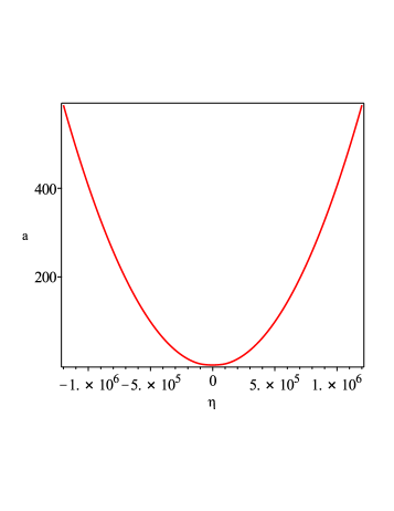
Figure 1: The evolution of the scale factor versus $\eta$. At bounce point ($\eta=0$), it gives a positive non-zero value

IV Bouncing with Running vacuum model

The running vacuum energy in quantum field theory (QFT) in curved space-time motivated us to consider $\rho_{\Lambda}=\Lambda(H)$ in reduced Planck mass unit. This theory gives the renormalization group equation Basilakos et al. (2012)

$$\frac{d\rho_{\Lambda}}{d\ln(\mu^{2})}=\frac{1}{4\pi}\left(\sum_{i}{B_{i}M_{i}\mu^{2}}+\sum_{i}{C_{i}\mu^{4}}+...\right),$$ (13)

where $\mu^{2}$ can be a linear combination of $H^{2}$ and $\dot{H}$ Sola and Gomez-Valent (2015), $B_{i}$ and $C_{i}$ are dimensionless coefficients and $M_{i}$ is the mass of any particle which contribute in the dynamics.

By setting $\mu^{2}=H^{2}$, the equation (13) simply yields

$$\rho_{\Lambda}(H^{2})=n_{0}+n_{2}H^{2}+n_{4}H^{4}+O(H^{6}).$$ (14)

However in general, by consideration of correction of QFT, a theoretical explanation of RVM-DE becomes (Sola (2013); Sola and Gomez-Valent (2015); Sola et al. (2017) and reference therein)

$$\rho_{\Lambda}(H^{2},\dot{H})=n_{0}+n_{2}H^{2}+\beta\dot{H}+n_{4}H^{4}+O(H^{6}).$$ (15)

The terms with higher powers of Hubble function have recently been used to describe inflation Sola (2013); Basilakos et al. (2013, 2014); Lima et al. (2016); Sola (2015). For $n_{i}=\beta=0;~{}~{}i=1,2,3,...$, the standard $\Lambda$CDM is recovered. On the other hand any model with a linear term of Hubble function motivated from a phenomenological point of view Schutzhold (2002); Thomas et al. (2009); Urban and Zhitnitsky (2010); Urban and Zhitnitsky (2009a, b); Klinkhamer and Volovik (2009). This model can still be tenable if a constant additive term is around Gomez-Valent and Sola (2015). It must be mentioned that a model of vacuum energy in which the density is just proportional to $H$ can not come from any covariant QFT and it does not even have a well-defined $\Lambda$CDM limit and the worst, it is also excluded from the data on structure formation Gomez-Valent and Sola (2015).

In following we are also interested to add another term $n_{1}H$ into Eq. (15) and studying on the role of each terms on evolution of the scale factor, density parameters, Hubble parameter and equation of state parameter in some cases and compare them with the $\Lambda$CDM bouncing model.

V cosmological Perturbation theory

The dynamics of scalar perturbations on a spatially flat background spacetime are explained by the Mukhanov-Sasaki equation with a gauge invariant variable $v=z\mathcal{R}$ Mukhanov et al. (1992) in which $\mathcal{R}$ is the comoving curvature perturbation and

$$z=\frac{a\,\sqrt{\rho_{tot}+P_{tot}}}{c_{s}\,H}=\frac{a\,(1+w)^{1/2}\,}{c_{s}}\frac{\sqrt{\rho_{tot}}}{H}.$$ (16)

Linear perturbations can be extended into LQC Salopek and Bond (1990); Wands et al. (2000). The LQC effective equation for the Mukhanov-Sasaki variable is Wilson-Ewing (2012a, b)

$$v^{\prime\prime}-c_{s}^{2}\,\left(1-\frac{2\rho_{tot}}{\rho_{c}}\right)\nabla^{2}v-\frac{z^{\prime\prime}}{z}v=0,$$ (17)

where $c_{s}$ is the speed of sound which is a constant parameter depending on every epoch of history of the universe. The effective equation (17) is expected to provide a good approximation to the full quantum dynamics for modes that always remain large compared to the Planck length Rovelli and Wilson-Ewing (2014). It must be noted that for $\rho_{c}\to\infty$, the standard classical perturbation equation is recovered Mukhanov (2005). Also the Holonomy-corrected tensor perturbation in LQC is Cailleteau et al. (2012):

$$\mu^{\prime\prime}-\,\left(1-\frac{2\rho_{tot}}{\rho_{c}}\right)\nabla^{2}\mu-\frac{z_{T}^{\prime\prime}}{z_{T}}\mu=0,$$ (18)

where $\mu=h\,z_{T}$ in which

$$z_{T}=\frac{a}{\sqrt{1-2\rho/\rho_{c}}}.$$ (19)

V.1 Analytical Solutions with case $\rho_{\Lambda}=n_{2}H^{2}+\beta\dot{H}$

Following Cai and Wilson-Ewing (2015), we consider three continues era for studying on scalar perturbation and power spectrum in analytical method. Modes of interest are those that reach the long wave length limit during the first era where it is very far from the bounce in which the evolution of the contracting universe treats as matter-dark energy domination. Then after equality of radiation with previous pair components, the universe enters to a radiation domination epoch and at last, goes through the bounce where the evolution of the universe governed by LQC.

Far enough the bounce, where quantum gravity effects are negligible, effective equations are standard Friedmann equations

$$3H^{2}=\rho,$$

$$\dot{\rho}=-3H\rho(1+w),$$ (20)

$$\dot{H}=\dfrac{-3}{2}H^{2}(1+w),$$ (21)

where we are using $\rho$ instead of $\rho_{tot}$ for simplicity. From above equations, the EoS parameter can be found simply as

$$w=w_{0}=-\frac{2n_{2}-3\beta}{6-3\beta}.$$ (22)

It is important to note that in a matter-dark energy dominated epoch, in order to have a nearly scale invariant power spectrum, the effective EoS parameter $w_{0}$ must be slightly negative.

Fortunately, we can directly calculate power spectrum and spectral index same as Mukhanov’s method of inflationary scenario, in conformal time Mukhanov (2005). Very far from the bounce, using (20), the $z$ quantity in (16) reduced to

$$z=a\sqrt{3}\left(\frac{\sqrt{1+w_{0}}}{c_{s}}\right),$$ (23)

and the Mukhanov-Sasaki equation for scalar perturbations (17) in Fourier modes will be rewritten as

$$v^{\prime\prime}+(c_{s}^{2}\,k^{2}-\frac{a^{\prime\prime}}{a})\,v=0.$$ (24)

Solving second Friedmann equation (21) in conformal time

$$\mathcal{H}^{\prime}=-\frac{\mathcal{H}^{2}}{2}(1+3w_{0}),$$ (25)

yields

$$\mathcal{H}=\frac{2}{(1+3w_{0})(\eta-\eta_{0})},$$ (26)

where $\eta_{0}$ is the constant of integration. Taking $a^{\prime\prime}/a=\mathcal{H}^{\prime}+\mathcal{H}^{2}$ and for very small values of $w_{0}$, the Mukhanove-Sasaki equation (24) approximately yields

$$v^{\prime\prime}+\left(c_{s}^{2}k^{2}-\dfrac{\nu^{2}-\dfrac{1}{4}}{(\eta-\eta_{0})^{2}}\right)v=0,$$ (27)

where $\nu=(9/4-18w_{0})^{1/2}\approx 3/2-6w_{0}+O(w_{0}^{2})$. The relevant solution is

$$v_{k}=\sqrt{|\eta-\eta_{0}|}\left(C_{1}\,H^{(1)}_{\nu}\left(c_{s}k|\eta-\eta_{0}|\,\right)+C_{2}\,H^{(2)}_{\nu}\left(c_{s}k|\eta-\eta_{0}|\,\right)\right).$$ (28)

Assuming the initial conditions of primordial perturbations in the distant past of the pre-bounce epoch, to be quantum vacuum states, it takes

$$v_{k}=\frac{{1}}{\sqrt{2c_{s}k}}e^{-i\,c_{s}k\ \eta}.$$ (29)

Using the asymptotic behavior of the first type of the Hankel function when $|\eta-\eta_{0}|>>0$

$$H^{(1)}_{\nu}\left(c_{s}k|\eta-\eta_{0}|\,\right)=\frac{\sqrt{2}\,e^{-(\nu+\frac{1}{2})\frac{\pi}{2}}}{\sqrt{c_{s}k\pi|\eta-\eta_{0}|}}\,e^{i\,c_{s}k|\eta-\eta_{0}|},$$ (30)

in solution (28), we find

$$C_{1}=\frac{\sqrt{\pi}}{2}e^{i(\nu+\frac{1}{2})\frac{\pi}{2}};~{}~{}~{}C_{2}=0.$$ (31)

In long wavelength limit, $c_{s}k|\eta-\eta_{0}|<<1$ and small values $|w_{0}|$, the solution reduced to

$$v_{k}\cong\frac{-i}{2}\sqrt{\frac{1}{2}}\,(c_{s}k)^{-3/2+6w_{0}}\left(\mathcal{H}\right)^{1-6w_{0}}.$$ (32)

In second step, after equality, before the quantum gravity effects become considerable, the evolution of the universe tends to radiation dominated epoch in which $w=1/3$, $c_{s}=\sqrt{1/3}$ and $\rho_{tot}=\rho_{0r}/a^{4}$. Also Eq. (9) in the limit $\rho_{c}\rightarrow\infty$, gives

$$a(\eta)=\sqrt{\frac{\rho_{0r}}{3}}\eta;~{}~{}~{}~{}~{}\mathcal{H}=\frac{1}{\eta}.$$ (33)

The perturbation equation reduces to a harmonic oscillator

$$v^{\prime\prime}+c_{s}^{2}k^{2}v=0,$$ (34)

with the following solution

$$v_{k}=B_{1}\sin(\frac{k}{\sqrt{3}}\eta)+B_{2}\cos(\frac{k}{\sqrt{3}}\eta).$$ (35)

Since this step is between dark matter-energy domination era and bounce period, hence in order to continue with the bounce period ($\eta\rightarrow 0$), the coefficient $B_{2}$ will dominate and hence it requires $B_{1}=0$. On the other hand the continuity of $v_{k}$ and $v_{k}^{\prime}$ at equality time $\eta_{e}$, gives

$$B_{2}=-\frac{\sqrt{3}}{k}\sin(\frac{k}{\sqrt{3}}\eta_{e})v_{k}^{\prime}|_{\eta=\eta_{e}}+\cos(\frac{k}{\sqrt{3}}\eta_{e})v_{k}|_{\eta=\eta_{e}},$$ (36)

and after substituting (32) and its derivative into (36) it goes

$$B_{2}= -\frac{i\sqrt{3}(c_{s}k)^{-3/2+6w_{0}}}{4\sqrt{2}k}\sin(\frac{k}{\sqrt{3}}\eta_{e})\mathcal{H}_{e}^{2-6w_{0}}$$

$$-\frac{i(c_{s}k)^{-3/2+6w_{0}}}{2\sqrt{2}}\cos(\frac{k}{\sqrt{3}}\eta_{e})\mathcal{H}_{e}^{1-6w_{0}}.$$ (37)

An essential condition for scale invariant power spectrum is $k|\eta_{e}|<<1$ Cai and Wilson-Ewing (2015). Therefor, in this approximation, $B_{2}$ simplify to

$$B_{2}\cong-\frac{3i}{4}\sqrt{\frac{1}{2}}(c_{s}k)^{-3/2+6w_{0}}\mathcal{H}_{e}^{1-6w_{0}}.$$ (38)

At last, in the bounce period, since the radiation is yet a dominant term ($w=1/3$), the first LQC effective equation in conformal time gives

$$\mathcal{H}^{2}=\frac{\rho_{0r}}{3a^{2}}(1-\frac{\rho_{0r}}{\rho_{c}a^{4}}),$$ (39)

which directly gives the following scale factor

$$a=(a_{0}t^{2}+1)^{1/4},$$ (40)

where $a_{0}={4\rho_{c}}/3$. On the other hand, from (17), the perturbation equation in conformal time becomes

$$\frac{v^{\prime\prime}}{v}-\frac{z^{\prime\prime}}{z}=0,$$ (41)

with following solution

$$v(t)=\frac{C_{1}a_{0}}{4\sqrt{\rho_{c}}}\,z\,\,t^{3}F\left(\frac{3}{2},\,\frac{7}{4},\,\frac{5}{2},\,-a_{0}t^{2}\right)+\frac{a_{0}z}{4\sqrt{\rho_{c}}},$$ (42)

after using (40). Its asymptotic behavior governs

$$\mathcal{R}\cong\frac{v_{k}}{z}=\frac{2A_{1}a_{0}^{-3/4}\sqrt{2\pi^{3}}}{z\Gamma(\frac{3}{4})^{2}}=\frac{1}{6}\sqrt{\frac{\pi}{3}}\frac{\Gamma(\frac{1}{4})}{\Gamma(\frac{3}{4})}B_{2},$$ (43)

where

$$A_{1}=-\frac{a_{0}B2}{6}.$$ (44)

Thus the power spectrum for modes that become (nearly) scale invariant in which $k|\eta_{e}|<<1$, is given by

$$\Delta^{2}=\frac{k^{3}\,|\mathcal{R}|^{2}}{2\pi^{2}}=\frac{1}{768}\left(\frac{\Gamma(\frac{1}{4})}{\Gamma(\frac{3}{4})}\right)^{2}c_{s}^{-3+12w_{0}}\mathcal{H}_{e}^{2-12w_{0}}\,k^{12w_{0}}.$$ (45)

It is worthwhile to mention that these modes must also remain outside the sound Hubble radius during the entire the contracting radiation dominated epoch and bounce period as well as dark matter-energy domination contracting era.

At the end, from (33), power spectrum can be rewritten as

$$\Delta^{2}=\frac{k^{3}\,|\mathcal{R}|^{2}}{2\pi^{2}}=\frac{1}{768}\left(\frac{\Gamma(\frac{1}{4})}{\Gamma(\frac{3}{4})}\right)^{2}c_{s}^{-3+12w_{0}}\left(\left(\frac{\rho_{c}}{3}\right)^{1/4}\sqrt{H_{e}}\right)^{2-12w_{0}}\,k^{12w_{0}}.$$ (46)

Obviously, if we set $w_{0}=0$, the power spectrum will be exactly scale-invariant, but for a small negative value of $w_{0}$, it is nearly scale-invariant with a red tilt for spectral index as it is predicted by observational data ($n_{s}=1+12w_{0}$)

In this section we study the Fourier modes evolution which they come from initial quantum vacuum state far away the bounce. Any mode that exit the sound Hubble radius in matter-dark domination period becomes scale invariant and they return to sound Hubble radius after the bounce, in expanding branch.

VI Spectral Index and its Running

Considering the semi-matter dominated epoch in contracting phase of the deformed matter bounce scenario. Far from the bounce point, the EoS parameter becomes very small $(w<<1)$ and approximately constant. Its time derivative is very small $(w^{\prime}<<1)$ around the crossing time, when the sound horizon crossed by long wavelength modes (e.g. see Fig. 3). It gives a good condition to solve the perturbation equation analytically and consequently obtains a simple relation for the power spectrum index (same as the previous section). Expanding the parameter $w$ around $\eta_{0}$ up to first order

$$w\approx w_{0}+\kappa(\eta-\eta_{0}),$$ (47)

where $\kappa=dw/d\eta$ at $\eta=\eta_{0}$ and $w_{0}$ is the value of $w$ at $\eta_{0}$. Since the changes of $w$ is very small, $|\Delta w|\approx|w-w_{0}||\kappa(\eta-\eta_{0})|<<1$, therefore during the semi-matter dominated epoch in a contraction phase, at low curvature and energies, in Eq. (17) we have $\frac{z^{\prime\prime}}{z}\cong\frac{a^{\prime\prime}}{a}$ (details are referred to Elizalde et al. (2015)).

Now by this approximation, the conformal Hubble parameter and $a^{\prime\prime}/a$ are calculated as

$$\mathcal{H}=\frac{4}{3\kappa(\eta-\eta_{0})^{2}+2(3w_{0}+1)(\eta-\eta_{0})},$$ (48)

$$\frac{a^{\prime\prime}}{a}\cong\frac{2-18w_{0}}{(\eta-\eta_{0})^{2}}-\frac{12\kappa}{\eta-\eta_{0}}.$$ (49)

By setting $\nu\cong 3/2-18w_{0}$ and $\xi=12\kappa$, the scalar perturbation equation (17) in Fourier mode becomes

$$v^{\prime\prime}+c_{s}^{2}k^{2}\left(1-\dfrac{\nu^{2}-\dfrac{1}{4}}{c_{s}^{2}k^{2}(\eta-\eta_{0})^{2}}+\frac{\xi(\eta-\eta_{0})}{c_{s}^{2}k^{2}(\eta-\eta_{0})^{2}}\right)v=0.$$ (50)

It is worthwhile to mention that in limiting case, when $|\xi(\eta-\eta_{0})|\rightarrow 0$, the above equation reduced to Eq. (27) in the previous section.

For convenience in calculations, we replace $\eta-\eta_{0}$ in (50) with $\eta$,

$$v^{\prime\prime}+\left(c_{s}^{2}k^{2}-\frac{\nu^{2}-\dfrac{1}{4}}{\eta^{2}}+\frac{\xi}{\eta}\right)v=0.$$ (51)

General answerer of this equation is

$$v\,=J_{1}\,W\left(\frac{-i\,\xi}{2\,c_{s}\,k},\,\nu\,,2\,i\,c_{s}\,k\,\eta\right)+J_{2}\,M\left(\frac{-i\,\xi}{2\,c_{s}\,k},\,\nu\,,2\,i\,c_{s}\,k\,\eta\right),$$ (52)

where $W$ and $M$ are Whittaker functions and $J_{i}$’s are constants of integration. By considering the asymptotic behavior of $W$ at large $|k\eta|$,

$$W\left(\frac{-i\,\xi}{2\,c_{s}\,k},\,\nu\,,2\,i\,c_{s}\,k\,\eta\right)\sim\exp(-i\,c_{s}\,k\eta)(-2ic_{s}\,k\eta)^{-i\xi/(2c_{s}k)},$$ (53)

and taking the initial condition of primordial perturbations to be quantum vacuum states, we find $J_{2}=0$ and

$$J_{1}=\sqrt{\frac{1}{2c_{s}k}}\exp(\frac{\pi\xi}{4c_{s}k}).$$

Now in the long wavelength limit, around the crossing horizon where $(|c_{s}k\eta|<<1)$, the solution of (52) rewritten as

$$v =\sqrt{\frac{1}{2c_{s}k}}\,\,\exp(\frac{\pi\xi}{4c_{s}k})\frac{\Gamma(2\nu)}{\Gamma\left(1/2+\nu+\dfrac{i\xi}{2c_{s}k}\right)}\,(2\,i\,c_{s}k\,\eta)^{1/2-\nu}$$

$$\cong\frac{-i}{2}\sqrt{\frac{1}{2c_{s}k}}\exp(\frac{\pi\xi}{4c_{s}k})\,\,(\frac{1}{2}c_{s}\,k\,\eta)^{-1+6w_{0}},$$ (54)

which it will reduce to Eq. (32) limiting case $\xi\rightarrow 0$.

Now, completely similar to the previous section, since the perturbations must be continued during the contraction and expansion of the universe, after forward calculation, the power spectrum $\Delta^{2}$ will be modified by coefficient $C(k)=\exp[\pi\xi/(2c_{s}k)]$ as follows

$$\Delta^{2}(k)\sim\exp(\frac{\pi\xi}{2c_{s}k})\,\,k^{12w_{0}}.$$ (55)

The spectral index in this case becomes

$$n_{s}-1=\frac{\,\mathrm{d}ln\Delta^{2}}{\,\mathrm{d}lnk}=-\frac{\pi\xi}{2c_{s}k}+12w_{0}.$$ (56)

Also to obtain the running of spectral index, as we will also be pointed out later,

$$\alpha_{s}=\frac{\,\mathrm{d}n_{s}}{\,\mathrm{d}\ln k}=\frac{\pi\xi}{2c_{s}k}=\frac{6\pi\kappa}{c_{s}k}.$$ (57)

An interesting point of this relation is obviously if $\kappa=dw/d\eta<0$, at any time, especially at crossing time, this running becomes negative. This point will be hinted again at next sections. Another point is about the value of the running of spectral index. From the observational data, $\alpha_{s}$ is very small and negative. Therefore, it is required that in the long wavelength limit,

$$|\frac{\pi\xi}{2c_{s}k}|\ll 1\Rightarrow|\xi(\eta-\eta_{0})|\ll|c_{s}k(\eta-\eta_{0})|\ll 1,$$ (58)

which again it emphasizes that the second term in Eq. (47) is very small in a semi-matter bounce scenario.

Finally, the Eq. (56) at the crossing Hubble horizon, will be rewritten as

$$n_{s}=1+12(w_{0}+\frac{|\alpha_{sc}|}{12})\approx 1+12w,$$ (59)

where $\alpha_{sc}$ is the running of spectral index at the crossing Hubble horizon which is a very small negative value, approximately same as the role of $|\kappa(\eta-\eta_{0})|$ in Eq. (47). Also Eq. (59) will reduce to $n_{s}=1+12w_{0}$ for constant EoS parameter of DE-model and vanishing $\alpha_{s}$, same as the previous section. It is worthwhile to mention again that we concentrate our attention to semi-matter bounce scenario which has a very small values of EoS parameter at whole of the contracting phase.

Moreover with this assumption, when a mode is crossed by Hubble radius, by using (59), the running of spectral index yields (details are referred to de Haro and Cai (2015)),

$$\alpha_{sc}=\left(\frac{dn_{s}}{d\ln k}\right)_{k=a|H|}=\left(\frac{dn_{s}}{dt}\frac{dt}{d\ln k}\right)_{k=a|H|}=\frac{12H\dot{w}}{H^{2}+\dot{H}}.$$ (60)

In a RVM model, in which $P_{D}=-\rho_{D}$, far enough the bounce, from the first Friedmann equation, the effective EoS parameter gives

$$w=-\frac{\rho_{\Lambda}}{\rho_{\Lambda}+\rho_{m}}=-\frac{\rho_{\Lambda}}{3H^{2}},$$ (61)

and after some calculations, $\dot{w}$ becomes

$$\dot{w}=\frac{\dot{\rho_{\Lambda}}}{\rho_{\Lambda}}w+3Hw(1+w).$$ (62)

Using Eqs. (61) and (21), the Eq. (62) will be rewritten by

$$\dot{w}=\frac{H^{2}(w+1)}{2}\frac{d}{dH}\left(\frac{\rho_{\Lambda}}{H^{2}}\right).$$ (63)

According to $|w|<<1$, $w$ is neglected and $\alpha_{s}$ becomes

$$\alpha_{s}\cong-12H\frac{d}{dH}\left(\frac{\rho_{\Lambda}}{H^{2}}\right),$$ (64)

so, approximately, the relation (64) can be rewritten by the following simple form

$$\alpha_{s}\cong 3H\frac{dn_{s}}{dH}.$$ (65)

In agreeing with the $\Lambda$CDM bouncing modelCai et al. (2016b), if $\rho_{\Lambda}=n_{0}$, from (64), we can see that the running of the spectral index becomes positive which is an obvious weakness of this case. Note that the effective equation of state parameter is negative in contracting phase of the universe at crossing time. In this case $\alpha_{s}$ approximately given by

$$\alpha_{s}=24\frac{n_{0}}{H^{2}}=-72w,$$ (66)

which gets a positive value for $w<0$.

For a constant effective EoS parameter, same as previous case (Eq. (22)), running of spectral index is vanishing which is in contrast with Planck bound Ade et al. (2016a, b). It is worthwhile to mention that also in the standard cosmology this type of RVM-DE (model of Sec. V) has been already excluded on account of its inability to correct description of the data on structure formation Gomez-Valent et al. (2015a); Gomez-Valent and Sola (2015); Gomez-Valent et al. (2015b). Thus this fact give us an alternative reason to exclude this type of RVM-DE.

In order to have a negative value of running of spectral index, ($\alpha_{s}<0$), which is compatible with the inflationary paradigm, it is required that $H\frac{d}{dH}(\rho_{\Lambda}/H^{2})>0$ (see Eq. (64)).

At following we will give two other cases of RVM and will calculate the spectral index and running.

VI.1 Case $\rho_{\Lambda}=n_{0}+n_{2}H^{2}$

This is one of the known cases of RVM which has been studied by many authors in standard cosmology Sola (2008); Basilakos et al. (2009); Espana-Bonet et al. (2004); Shapiro and Sola (2004); Basilakos et al. (2012). In bouncing scenario, according to previous section, far enough the bounce point, when the sound horizon crossed by long wavelength modes, from (59) and (64), we will have

$$n_{s}-1=-12(\frac{n_{0}}{3H_{cr}^{2}}+\frac{n_{2}}{3}),$$ (67)

and the running will be

$$\alpha_{s}=24\frac{n_{0}}{H_{cr}^{2}},$$ (68)

where $H_{cr}$ is the value of the Hubble parameter at crossing time ($\eta=\eta_{c}$). As a result, $\alpha_{s}$ is always positive unless $n_{0}<0$. However a negative value of $n_{0}$ is forbidden near the bounce point where $H\approx 0$ and consequently $\rho_{\Lambda}\approx n_{0}$.

VI.2 $\rho_{\Lambda}=n_{0}+n_{2}H^{2}+n_{4}H^{4}$

The first attempts to consider this type of RVM which was extended to $H^{4}$ term in standard cosmology was given by in Lima et al. (2013). In this case the effective EoS parameter is simply calculated as

$$w_{0}=\frac{n_{s}-1}{12}=-\frac{1}{3}\left(\frac{n_{0}}{H_{cr}^{2}}+{n_{2}}{}+{n_{4}}{}H_{cr}^{2}\right),$$ (69)

and from Eq. (64) the running $\alpha_{s}$ is

$$\alpha_{sc}=24\left(\frac{n_{0}}{H_{cr}^{2}}-n_{4}H_{cr}^{2}\right).$$ (70)

Obviously in order to have $\alpha_{sc}<0$, it requires that

$$n_{4}>\frac{n_{0}}{H_{cr}^{4}}.$$ (71)

Simply after some algebraic calculation, the relation between $n_{0}$, $n_{2}$ and $n_{4}$, can be found as

$$n_{2}=\frac{6-6n_{s}-\alpha_{sc}}{24}-\frac{2n_{0}}{H_{cr}^{2}},$$ (72)

$$n_{4}=\frac{n_{0}}{H_{cr}^{4}}-\frac{\alpha_{sc}}{24H_{cr}^{2}}.$$ (73)

These relations can help us to estimate the order of magnitude of parameters of this case to find benefit numerical calculations at next.

It is important to note that in cosmological perturbation theory, the power spectrum, spectral index and its running essentially depend on the effective equation of state and its derivative at time of horizon-crossing. In other words, in the contracting phase, the space-time curvature is not felt by the Fourier modes inside the horizon, so they oscillate until exiting inside the horizon. The background spacetime evolution, equation of state and the time derivative of $w$ at the horizon-crossing in matter dominate epoch have an important role to appropriate predict of nearly scale-invariant power spectrum and the running of the spectral index. Now we ask, is it possible to have a negative running of the spectral index in matter bounce scenario in this case?

To answer this question, firstly, we interested to solve numerically the background differential equations (8, 9, 10).

VI.2.1 background numerical calculation

By using Eqs. (72), (73), and the requirement of negative running in (70), a set of parameters can be estimated as

$$n_{0}=2.2\times 10^{-28}\,\,\,\,\,\,\,n_{2}=8.9\times 10^{-3}\,\,\,\,\,\,\,n_{4}=4.47\times 10^{10}\,.$$ (74)

It is worthwhile to mention that in reduced Planck mass units, $\rho_{\Lambda}$ has dimension $H^{2}$ and $\dot{H}$, i.e. inverse length squared, (see Eqs. (3, 4)) and consequently time, length and mass get equal dimension. Therefore in this case, the constant parameter $n_{0}$ has dimension $H^{2}$, the coefficient of $H^{2}$, $n_{2}$, is dimensionless and the coefficient of $H^{4}$, $n_{4}$, has dimension $H^{-2}$ (length squared). Also, we must note that this set of parameters achieved approximately by a rough estimating of constrained values of $\alpha_{sc}$, $n_{s}$ and the calculated value of $H_{cr}$ at $\eta_{c}$. These coefficients satisfy inequality (71) and reminded that in bounce point the universe is dominated by radiation. The evolution of the scale factor, as expected, similar to fig.1, shows an expansion after contraction through the critical bounce point without any singularity.

The evolution of the conformal Hubble rate is indicated in fig. 2. The value of $\mathcal{H}$ is decreasing into a minimum value when $\eta\approx-1\times 10^{5}$. After that, $\mathcal{H}$ increases very fast and the universe evolves under a bouncing from a negative valued regime to the positive one. Eventually, after reaching to a maximum value at $\eta\approx 1\times 10^{5}$, the value of $\mathcal{H}$ decreases in the expanding universe. Due to this form of evolution of $\mathcal{H}$, we give a discussion about the strength of each term of $\rho_{\Lambda}$ in any epoch of the universe. As we found from Eq. (74), the parameter $n_{4}$ is about 38 orders of magnitude greater than $n_{0}$ and about 13 orders of magnitude greater than $n_{2}$. Also $n_{2}$ is about 25 orders of magnitude greater than $n_{0}$. Therefor at bounce point where $H=0$, the only non vanishing term is $n_{0}$. After that, up to $\eta\approx 1\times 10^{5}$, the term $n_{4}H^{4}$ would be a dominant term, but it will be diluted as the universe goes on ($\mathcal{H}$ decreased very fast) so that at a far future of bouncing, again the term $n_{0}$ will be dominated.

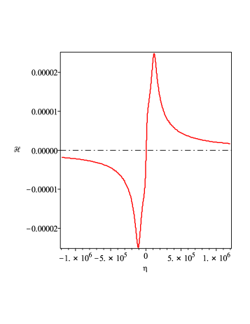
Figure 2: The evolution of the conformal Hubble parameter $\mathcal{H}$ versus $\eta$. At bounce point ($\eta=0;~{}~{}\mathcal{H}=0$), it shows a transition from a contracting universe to an expanding one from left to right.

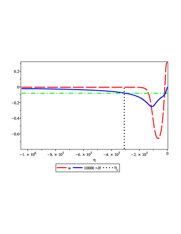
Figure 3: The evolution of the conformal Hubble parameter $\mathcal{H}$ (Solid blue line) and equation of state parameter $w$ (dash red line), versus conformal time $\eta$ for the case contained $H^{4}$. Green dot-dash line is the crossing Hubble parameter $\mathcal{H}_{cr}$ which is occurred by crossing the conformal time, $\eta_{c}$ with curve $\mathcal{H}$.

The evolution of the EoS parameter has been shown in fig. 3 (red dash line). As one can see, in the $\Lambda$CDM epoch, $w$ is very close to a constant small negative value $w\sim-0.003$. This is very good condition for getting a red tilt in the spectral index as indicated in (59). In continuing along the conformal time about $\eta_{d}\approx-3.4\times 10^{5}$, $w$ decreases and after this point the time derivative of $w$ becomes negative. It is reasonable to expect that after this point, dark energy has been dominated again gradually. This decreasing behavior is continuing until $w$ reaches to a minimum value ($w=-0.65$) at $\eta\approx-6\times 10^{4}$. After this point, the radiation component will be dominated. It should be noted that in contracting phase ($\mathcal{H}<0$), Eqs. (63) and (64) yields

$$\alpha_{s}\sim-\frac{24w^{\prime}}{\mathcal{H}},$$ (75)

which will give a negative value of spectral index for all negative values of $w^{\prime}$ and $\mathcal{H}$ at crossing time.

The evolution of the conformal Hubble parameter $\mathcal{H}$ has been also shown (blue solid line) in fig. 3. In this figure, the green horizontal dash-dot line shows the sound-Hubble horizon in Fourier mode $k=9.7\times 10^{-5}$. Same as Cai and Wilson-Ewing (2015), we chose the speed of sound, $c_{s}=0.08$ and consequently $|\mathcal{H}_{cr}|=c_{s}k=7.7\times 10^{-6}$ is the amount of radius of sound-Hubble horizon. Crossing time is indicated by vertical dot line. As it shows, this line cross the curve $\mathcal{H}$ at $\eta_{c}\approx-3.1\times 10^{5}$, which it occurs after $\eta_{d}$. This means that the derivative of $w$ at the crossing time gets a negative value. In this time, $w=w_{cr}\approx-0.0029$, $n_{s}=12w_{cr}+1\approx 0.96$ and after some numerical calculation we obtain $\alpha_{sc}\approx-0.003$, which has a very good consistency with constrained results ($\alpha_{sc}=-0.003\pm 0.007$ by $68\%$ CL, Planck+TT+LowP+Lensing Ade et al. (2016b)). In fig. 4, using Eq. (60), the behavior of the $\alpha_{s}$ has been clearly shown around the crossing time (solid red line). As it is shown in this figure, at the horizon-crossing time $\eta_{c}$, the running $\alpha_{s}$ gets a negative small value ($\alpha_{s}\approx-0.003$, see the horizontal green dash-dot line in Fig. 4).

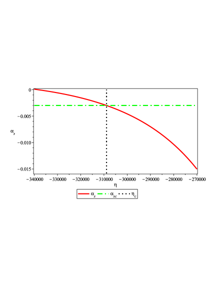
Figure 4: The behavior of $\alpha_{s}$ around the crossing time (solid line) which it is equal to $\alpha_{sc}$ at $\eta_{c}$

VI.2.2 perturbation in numerical calculation

The evolution of cosmological perturbation is governed by Eqs. (17) and (18). We are using a set of parameters of (74), which have been estimated in last subsection and setting Fourier mode $k=9.6\times 10^{-5}$. Also during the matter dominated contracting phase, we impose the initial conditions of the cosmological perturbation to be vacuum fluctuation. Furthermore, we have two matter components in our model (radiation and CDM). Since the speed of sound depends on the background evolution, in numerical computation, approximately, we divide the speed of the sound in two parts

$$c_{s}=\left\{\begin{array}[]{lr}\epsilon&w\simeq-0.003\\ \sqrt{w}&\,\,\,\,\text{radiation-dominated epoch}\end{array}\right.$$ (76)

which $\epsilon$ is equal to $0.08$ as mentioned previously.

The evolution of the scalar cosmological perturbation (blue dash line) has been depicted in fig. 5. As it can be seen, curvature perturbation oscillates from the sub-Hubble scale to super-Hubble region at $\eta_{c}\approx-3.1\times 10^{5}$, in which the oscillation finished. In fact $k$-mode curvature perturbation exits from the sound Hubble horizon at the crossing point $\eta_{c}$. As it shows, after equality time (vertical green line) when $\rho_{r}=\rho_{m}+\rho_{\Lambda}$, we can consider the radiation begins to dominate or in analytically point of view, ${z^{\prime\prime}}/{z}\rightarrow 0$, and consequently the amplitude of the scalar perturbation approximately becomes constant.

The red solid line shows the oscillation of the tensor cosmological perturbation or gravitational wave. The sound speed of the tensor perturbation is $c_{s}^{T}=1$. So clearly, tensor perturbation continue to oscillates even after vertical black dot line and eventually will damp to a constant value after equality time.

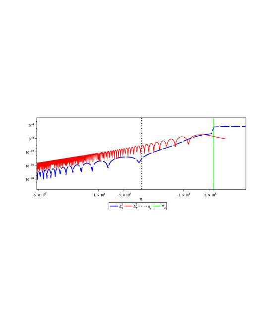
Figure 5: The evolution of scalar and tensor perturbation versus $\eta$ with $\epsilon=0.08$ for the case contained term $H^{4}$. Dash blue line indicates the scalar perturbation evolution and solid red line indicates the tensor perturbation evolution. Dot black line indicates the crossing time and vertical solid green line is referred to the equality time.

Besides the nearly scale invariant power spectrum with a negative running, a small tensor to scalar ratio is predicted by a cosmological bounce scenario. The tensor-to-scalar ratio $r$ is constrained by the observational bound ($r<0.12$) Ade et al. (2015). There are some known mechanisms for predicting a small tensor to scalar ratio Cai et al. (2013a, 2011b); Fertig et al. (2016); Wilson-Ewing (2016).

Actually, in our model, the speed of sound in matter dominated epoch is less than unity, so it affects on the amplitude of the scalar perturbations and consequently the amplitude of the scalar perturbation can be increased against the amplitude of the tensor perturbation. Also as it is shown in fig. 5, the discontinuity of $c_{s}$ about the equality time, suddenly increased the amplitude of the scalar perturbation. The evolution of tensor to scalar ratio $r$ is shown in fig. 6. As one can see, before the equality time (dot green line), the amount of tensor to scalar ratio $r$ slowly decreases from high to low.

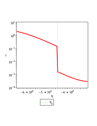
Figure 6: The evolution of tensor to scalar ratio ($r$) versus $\eta$ for the case contained term $H^{4}$. The ratio at $\eta_{e}$ suddenly decreased to $r\leq 0.001$.

In order to compare all studied cases of RVM-bounce scenario, we summarize all of them in table 1. As we found, for the cases 1-4, some physical requirements such as $\rho_{\Lambda}>0$ (or $n_{0}>0$) at any time and $w<0$ at the crossing time, required that $\alpha_{s}>0$. In the final column of the table 1, the value of $\alpha_{sc}$ is calculated for all cases at crossing time, where $w=w_{cr}=-0.003$, and $H=H_{cr}=-8.8\times 10^{-8}$ for $n_{0}>0$. At last, except the case contained the term $H^{4}$, other cases cannot satisfy the weak energy condition and observational evidence simultaneously. Therefore we excluded them in further numerical calculation analysis (such as tensor to scalar ratio $r$).

	$\rho_{\Lambda}$	$w=(n_{s}-1)/12$	$\dot{w}$	$\alpha_{s}$	$\alpha_{sc}$
— 1	$n_{0}$	$\dfrac{-n_{0}}{3H^{2}}$	$3Hw(1+w)$	$-72w$	0.22
— 2	$n_{0}+n_{2}H^{2}$	$-\dfrac{1}{3}(\dfrac{n_{0}}{H^{2}}+n_{2})$	$\dfrac{3n_{0}H}{n_{0}+n_{2}H^{2}}w(1+w)$	$\dfrac{n_{0}}{n0+n_{2}H^{2}}(-72w)$	0.22
— 3	$n_{0}+n_{1}H$	$-\dfrac{1}{3}(\dfrac{n_{0}}{H^{2}}+\dfrac{n_{1}}{H})$	$\dfrac{3H(n_{1}H+2n_{0})}{2n_{0}+n_{1}H}w(1+w)$	$\dfrac{n_{1}H+2n_{0}}{n_{1}H+n_{0}}(-72w)$	0.44
— 4	$n_{0}+\beta\dot{H}$	$\dfrac{2n_{0}/H^{2}-3\beta}{-6+3\beta}$	$\dfrac{3Hn_{0}w(1+w)}{n_{0}-3\beta H^{2}/2}$	$\dfrac{n_{0}}{n_{0}-3\beta H^{2}/2}(-72w)$	0.001
— 5	$n_{2}H^{2}+\beta\dot{H}$	$\dfrac{-2n_{2}+3\beta}{6-3\beta}$	0	0	0
— 6	$n_{0}+n_{2}H^{2}+n_{4}H^{4}$	$-\dfrac{1}{3}(\dfrac{n_{0}}{H^{2}}+n_{2}+n_{4}H^{2})$	$\dfrac{3H(-n_{4}H^{4}+n_{0})w(1+w)}{n_{0}+n_{2}H^{2}+n_{4}H^{4}}$	$\dfrac{(-n_{4}H^{4}+n_{0})(-72w)}{n_{0}+n_{2}H^{2}+n_{4}H^{4}}$	-0.003

Table 1: Summary of all cases in RVM-bounce scenario . Note that in all cases, $w$ has a small negative value (see Eq. (61)). Also the running $\alpha_{sc}$ is the value of $\alpha_{s}$ at crossing, $H=H_{cr}=-8.8\times 10^{-8}$ (in contracting phase) and $w=w_{cr}=-0.003$ provided that $\rho_{\Lambda}>0$ even at the bounce point ($\mathcal{H}=0$).

VII conclusion

In this work we introduced a deformed matter bounce scenario with the running vacuum model (RVM). This model could be considered as a viable alternative to the inflationary paradigm both in observational and theoretical aspects. Based on RVM-DE, the standard cosmological constant not more constant, but may consider as series of powers of $H^{2}$ and $\dot{H}$. By introducing some cases of RVM, we calculated the spectral index $n_{s}$ and its running $\alpha_{s}$ in order to compare with observational data. In fact in the contracting phase, before a bouncing, when the EoS parameter is slightly negative, Fourier modes of perturbations exit from the sound horizon. Thus power spectrum of cosmological perturbation for long wavelength modes is not exactly scale invariant and consequently it gets a slightly red tilt.

The process of creating of red tilt is obviously indicated in the analytical treatment for the case $\Lambda=n_{2}H^{2}+\alpha\dot{H}$. In this case the running of spectral index become vanishing, $\alpha_{s}=0$, which is inconsistent with inflationary paradigm. Some models with expansion up to $H^{2}$ got positive running and for a model $\Lambda(H)=n_{0}+n_{2}H^{2}+n_{4}H^{4}$, by estimating a set of parameters, we obtained the spectral index $n_{s}\approx 0.96$, running of spectral index $\alpha_{s}<0$ and tensor to scalar ratio $r<0.12$. We found that this model had the best consistency with the cosmological observations and reveals a degeneracy between deformed matter bounce scenario with RVM-DE and inflation. As a work in the future, the observational constraint of this model and comparison with cosmological observations are suggested.

References

- Hinshaw et al. (2013) G. Hinshaw et al. (WMAP), Astrophys. J. Suppl. 208, 19 (2013), eprint 1212.5226.
- Ade et al. (2014) P. A. R. Ade et al. (Planck), Astron. Astrophys. 571, A16 (2014), eprint 1303.5076.
- Hawking and Penrose (1970) S. W. Hawking and R. Penrose, Proc. Roy. Soc. Lond. A314, 529 (1970).
- Borde and Vilenkin (1994) A. Borde and A. Vilenkin, Phys. Rev. Lett. 72, 3305 (1994), eprint gr-qc/9312022.
- Martin and Brandenberger (2001) J. Martin and R. H. Brandenberger, Phys. Rev. D63, 123501 (2001), eprint hep-th/0005209.
- Brandenberger and Peter (2016) R. Brandenberger and P. Peter (2016), eprint 1603.05834.
- Brandenberger (2012) R. H. Brandenberger (2012), eprint 1206.4196.
- Finelli and Brandenberger (2002) F. Finelli and R. Brandenberger, Phys. Rev. D65, 103522 (2002), eprint hep-th/0112249.
- Gasperini and Veneziano (1993) M. Gasperini and G. Veneziano, Astropart. Phys. 1, 317 (1993), eprint hep-th/9211021.
- Khoury et al. (2001) J. Khoury, B. A. Ovrut, P. J. Steinhardt, and N. Turok, Phys. Rev. D64, 123522 (2001), eprint hep-th/0103239.
- Cai (2014) Y.-F. Cai, Sci. China Phys. Mech. Astron. 57, 1414 (2014), eprint 1405.1369.
- Brandenberger and Vafa (1989) R. H. Brandenberger and C. Vafa, Nucl. Phys. B316, 391 (1989).
- Nayeri et al. (2006) A. Nayeri, R. H. Brandenberger, and C. Vafa, Phys. Rev. Lett. 97, 021302 (2006), eprint hep-th/0511140.
- Lin et al. (2011) C. Lin, R. H. Brandenberger, and L. Perreault Levasseur, JCAP 1104, 019 (2011), eprint 1007.2654.
- Wilson-Ewing (2013) E. Wilson-Ewing, JCAP 1303, 026 (2013), eprint 1211.6269.
- Cai et al. (2016a) Y.-F. Cai, F. Duplessis, D. A. Easson, and D.-G. Wang, Phys. Rev. D93, 043546 (2016a), eprint 1512.08979.
- Cai et al. (2016b) Y.-F. Cai, A. Marciano, D.-G. Wang, and E. Wilson-Ewing, Universe 3, 1 (2016b), eprint 1610.00938.
- Cai et al. (2013a) Y.-F. Cai, E. McDonough, F. Duplessis, and R. H. Brandenberger, JCAP 1310, 024 (2013a), eprint 1305.5259.
- Cai and Wilson-Ewing (2014) Y.-F. Cai and E. Wilson-Ewing, JCAP 1403, 026 (2014), eprint 1402.3009.
- Bamba and Odintsov (2015) K. Bamba and S. D. Odintsov, Symmetry 7, 220 (2015), eprint 1503.00442.
- Odintsov and Oikonomou (2014) S. D. Odintsov and V. K. Oikonomou, Phys. Rev. D90, 124083 (2014), eprint 1410.8183.
- Haro and Amorós (2016) J. Haro and J. Amorós, PoS FFP14, 163 (2016), eprint 1501.06270.
- Boisseau et al. (2016) B. Boisseau, H. Giacomini, and D. Polarski, JCAP 1605, 048 (2016), eprint 1603.06648.
- Ashtekar and Singh (2011) A. Ashtekar and P. Singh, Class. Quant. Grav. 28, 213001 (2011), eprint 1108.0893.
- Ashtekar (2007) A. Ashtekar, Nuovo Cim. B122, 135 (2007), eprint gr-qc/0702030.
- Bojowald (2009) M. Bojowald, Class. Quant. Grav. 26, 075020 (2009), eprint 0811.4129.
- Cailleteau et al. (2012) T. Cailleteau, A. Barrau, J. Grain, and F. Vidotto, Phys. Rev. D86, 087301 (2012), eprint 1206.6736.
- Quintin et al. (2014) J. Quintin, Y.-F. Cai, and R. H. Brandenberger, Phys. Rev. D90, 063507 (2014), eprint 1406.6049.
- Cai et al. (2011a) Y.-F. Cai, S.-H. Chen, J. B. Dent, S. Dutta, and E. N. Saridakis, Class. Quant. Grav. 28, 215011 (2011a), eprint 1104.4349.
- Cai et al. (2011b) Y.-F. Cai, R. Brandenberger, and X. Zhang, JCAP 1103, 003 (2011b), eprint 1101.0822.
- Amorós et al. (2013) J. Amorós, J. de Haro, and S. D. Odintsov, Phys. Rev. D87, 104037 (2013), eprint 1305.2344.
- Qiu et al. (2013) T. Qiu, X. Gao, and E. N. Saridakis, Phys. Rev. D88, 043525 (2013), eprint 1303.2372.
- de Haro and Amoros (2014) J. de Haro and J. Amoros, JCAP 1408, 025 (2014), eprint 1403.6396.
- Cai et al. (2012) Y.-F. Cai, D. A. Easson, and R. Brandenberger, JCAP 1208, 020 (2012), eprint 1206.2382.
- Cai et al. (2013b) Y.-F. Cai, R. Brandenberger, and P. Peter, Class. Quant. Grav. 30, 075019 (2013b), eprint 1301.4703.
- Mukhanov and Brandenberger (1992) V. F. Mukhanov and R. H. Brandenberger, Phys. Rev. Lett. 68, 1969 (1992).
- Brandenberger et al. (1993) R. H. Brandenberger, V. F. Mukhanov, and A. Sornborger, Phys. Rev. D48, 1629 (1993), eprint gr-qc/9303001.
- Yoshida et al. (2017) D. Yoshida, J. Quintin, M. Yamaguchi, and R. H. Brandenberger, Phys. Rev. D96, 043502 (2017), eprint 1704.04184.
- Sami et al. (2006) M. Sami, P. Singh, and S. Tsujikawa, Phys. Rev. D74, 043514 (2006), eprint gr-qc/0605113.
- Ade et al. (2016a) P. A. R. Ade et al. (Planck), Astron. Astrophys. 594, A13 (2016a), eprint 1502.01589.
- Ade et al. (2016b) P. A. R. Ade et al. (Planck), Astron. Astrophys. 594, A20 (2016b), eprint 1502.02114.
- Lehners and Wilson-Ewing (2015) J.-L. Lehners and E. Wilson-Ewing, JCAP 1510, 038 (2015), eprint 1507.08112.
- Cai and Wilson-Ewing (2015) Y.-F. Cai and E. Wilson-Ewing, JCAP 1503, 006 (2015), eprint 1412.2914.
- Odintsov and Oikonomou (2016) S. D. Odintsov and V. K. Oikonomou, Phys. Rev. D94, 064022 (2016), eprint 1606.03689.
- Basilakos et al. (2012) S. Basilakos, D. Polarski, and J. Sola, Phys. Rev. D86, 043010 (2012), eprint 1204.4806.
- Sola (2016) J. Sola (2016), eprint 1601.01668.
- Sola et al. (2017) J. Sola , A. Gomez-Valent, and J. de Cruz Pérez, Astrophys. J. 836, 43 (2017), eprint 1602.02103.
- Fritzsch et al. (2017) H. Fritzsch, R. C. Nunes, and J. Sola, Eur. Phys. J. C77, 193 (2017), eprint 1605.06104.
- Sola et al. (2016) J. Sola, J. de Cruz Pérez, A. Gomez-Valent, and R. C. Nunes (2016), eprint 1606.00450.
- Sola et al. (2017) J. Sola, J. d. C. Perez, and A. Gomez-Valent (2017), eprint 1703.08218.
- Perico et al. (2013) E. L. D. Perico, J. A. S. Lima, S. Basilakos, and J. Sola, Phys. Rev. D88, 063531 (2013), eprint 1306.0591.
- Shapiro and Sola (2002) I. L. Shapiro and J. Sola, JHEP 02, 006 (2002), eprint hep-th/0012227.
- Ashtekar et al. (2006) A. Ashtekar, T. Pawlowski, and P. Singh, Phys. Rev. D74, 084003 (2006), eprint gr-qc/0607039.
- Sola and Gomez-Valent (2015) J. Sola and A. Gomez-Valent, Int. J. Mod. Phys. D24, 1541003 (2015), eprint 1501.03832.
- Sola (2013) J. Sola, J. Phys. Conf. Ser. 453, 012015 (2013), eprint 1306.1527.
- Basilakos et al. (2013) S. Basilakos, J. A. S. Lima, and J. Sola, Int. J. Mod. Phys. D22, 1342008 (2013), eprint 1307.6251.
- Basilakos et al. (2014) S. Basilakos, J. A. Sales Lima, and J. Sola , Int. J. Mod. Phys. D23, 1442011 (2014), eprint 1406.2201.
- Lima et al. (2016) J. A. S. Lima, S. Basilakos, and J. Sola , Eur. Phys. J. C76, 228 (2016), eprint 1509.00163.
- Sola (2015) J. Sola, Int. J. Mod. Phys. D24, 1544027 (2015), eprint 1505.05863.
- Schutzhold (2002) R. Schutzhold, Phys. Rev. Lett. 89, 081302 (2002), eprint gr-qc/0204018.
- Thomas et al. (2009) E. C. Thomas, F. R. Urban, and A. R. Zhitnitsky, JHEP 08, 043 (2009), eprint 0904.3779.
- Urban and Zhitnitsky (2010) F. R. Urban and A. R. Zhitnitsky, Phys. Lett. B688, 9 (2010), eprint 0906.2162.
- Urban and Zhitnitsky (2009a) F. R. Urban and A. R. Zhitnitsky, JCAP 0909, 018 (2009a), eprint 0906.3546.
- Urban and Zhitnitsky (2009b) F. R. Urban and A. R. Zhitnitsky, Phys. Rev. D80, 063001 (2009b), eprint 0906.2165.
- Klinkhamer and Volovik (2009) F. R. Klinkhamer and G. E. Volovik, Phys. Rev. D80, 083001 (2009), eprint 0905.1919.
- Gomez-Valent and Sola (2015) A. Gomez-Valent and J. Sola, Mon. Not. Roy. Astron. Soc. 448, 2810 (2015), eprint 1412.3785.
- Mukhanov et al. (1992) V. F. Mukhanov, H. A. Feldman, and R. H. Brandenberger, Phys. Rept. 215, 203 (1992).
- Salopek and Bond (1990) D. S. Salopek and J. R. Bond, Phys. Rev. D42, 3936 (1990).
- Wands et al. (2000) D. Wands, K. A. Malik, D. H. Lyth, and A. R. Liddle, Phys. Rev. D62, 043527 (2000), eprint astro-ph/0003278.
- Wilson-Ewing (2012a) E. Wilson-Ewing, Class. Quant. Grav. 29, 085005 (2012a), eprint 1108.6265.
- Wilson-Ewing (2012b) E. Wilson-Ewing, Class. Quant. Grav. 29, 215013 (2012b), eprint 1205.3370.
- Rovelli and Wilson-Ewing (2014) C. Rovelli and E. Wilson-Ewing, Phys. Rev. D90, 023538 (2014), eprint 1310.8654.
- Mukhanov (2005) V. Mukhanov, Physical Foundations of Cosmology (Cambridge University Press, Oxford, 2005), ISBN 0521563984, 9780521563987.
- Elizalde et al. (2015) E. Elizalde, J. Haro, and S. D. Odintsov, Phys. Rev. D91, 063522 (2015), eprint 1411.3475.
- de Haro and Cai (2015) J. de Haro and Y.-F. Cai, Gen. Rel. Grav. 47, 95 (2015), eprint 1502.03230.
- Gomez-Valent et al. (2015a) A. Gomez-Valent, J. Sola , and S. Basilakos, JCAP 1501, 004 (2015a), eprint 1409.7048.
- Gomez-Valent et al. (2015b) A. Gomez-Valent, E. Karimkhani, and J. Sola, JCAP 1512, 048 (2015b), eprint 1509.03298.
- Sola (2008) J. Sola, J. Phys. A41, 164066 (2008), eprint 0710.4151.
- Basilakos et al. (2009) S. Basilakos, M. Plionis, and J. Sola, Phys. Rev. D80, 083511 (2009), eprint 0907.4555.
- Espana-Bonet et al. (2004) C. Espana-Bonet, P. Ruiz-Lapuente, I. L. Shapiro, and J. Sola, JCAP 0402, 006 (2004), eprint hep-ph/0311171.
- Shapiro and Sola (2004) I. L. Shapiro and J. Sola, p. AHEP2003/013 (2004), [PoSAHEP2003,013(2003)], eprint astro-ph/0401015.
- Lima et al. (2013) J. A. S. Lima, S. Basilakos, and J. Sola, Mon. Not. Roy. Astron. Soc. 431, 923 (2013), eprint 1209.2802.
- Ade et al. (2015) P. A. R. Ade et al. (BICEP2, Planck), Phys. Rev. Lett. 114, 101301 (2015), eprint 1502.00612.
- Fertig et al. (2016) A. Fertig, J.-L. Lehners, E. Mallwitz, and E. Wilson-Ewing, JCAP 1610, 005 (2016), eprint 1607.05663.
- Wilson-Ewing (2016) E. Wilson-Ewing, Int. J. Mod. Phys. D25, 1642002 (2016), eprint 1512.05743.