KPZ modes in $d$-dimensional directed polymers

Abstract

We define a stochastic lattice model for a fluctuating directed polymer in $d\geq 2$ dimensions. This model can be alternatively interpreted as a fluctuating random path in 2 dimensions, or a one-dimensional asymmetric simple exclusion process with $d-1$ conserved species of particles. The deterministic large dynamics of the directed polymer are shown to be given by a system of coupled Kardar-Parisi-Zhang (KPZ) equations and diffusion equations. Using non-linear fluctuating hydrodynamics and mode coupling theory we argue that stationary fluctuations in any dimension $d$ can only be of KPZ type or diffusive. The modes are pure in the sense that there are only subleading couplings to other modes, thus excluding the occurrence of modified KPZ-fluctuations or Lévy-type fluctuations which are common for more than one conservation law. The mode-coupling matrices are shown to satisfy the so-called trilinear condition.
Keywords: Directed polymer, Exclusion process, KPZ equation, Non-linear fluctuating hydrodynamics

${}^{~{}1}$Institute of Complex Systems II, Forschungszentrum Jülich, 52425 Jülich, Germany
Email: g.schuetz@fz-juelich.de

² Purdue University, Department of Mathematics and Department of Physics and Astronomy, 150 N. University Street. West Lafayette, IN 47906, USA
Email: ebkaufma@math.purdue.edu

1 Introduction

The dynamics of one-dimensional many-body systems is presently a topic of intense study. One of the main motivations is to study anomalous transport phenomena which arise in different contexts and various physical scenarios even when interactions are short-ranged. Specific topics of interest are one-dimensional stochastic equations with local conservations laws (in particular for interface dynamics in the universality class of the one-dimensional noisy Kardar-Parisi-Zhang (KPZ) equation) and stationary spatio-temporal fluctuations in driven diffusion, or anharmonic chains or Hamiltonian fluid dynamics, see e.g. the collection of articles in [1] and in the first issue of volume 160 of the Journal of Statistical Physics (2015) for recent overviews. In the case of a single locally conserved quantity the long wave-length fluctuations of the conserved field are generally either diffusive with dynamical exponent $z=2$ or in the KPZ universality class [2] with dynamical exponent $z=3/2$.

In this article, we will focus on coupled one-dimensional stochastic equations with more than one conservation law. They show a much richer behavior than the single KPZ equation, depending on the details of the models. Fluctuations of the conserved fields can be in a modified KPZ universality class [3] or, more intriguingly, in a discrete family of Lévy universality classes [4] where the dynamical exponents $z_{i}$ are the Kepler ratios of neighbouring Fibonacci numbers and the universal scaling forms of the dynamical structure function are $z_{i}$-stable Lévy distributions. The first member in this family is a mode with dynamical exponent $z=3/2$ as in KPZ, but Lévy scaling function which very recently was proved rigorously for energy fluctuations in a harmonic chain with energy-conserving noise [5]. The second member with dynamical exponent $z=5/3$ was first firmly established using mode coupling theory for the heat mode in Hamiltonian dynamics for a one-dimensional fluid [6]. Also the limiting value of the Kepler ratios, which is the famous golden mean, can arise [3, 4, 7].

Here we address the nature of the dynamical structure functions in a higher dimensional setting, viz. for the contour fluctuations in a lattice model for a directed polymer in $d\geq 2$ dimensions, somewhat in the spirit of the space-continuous polymer model of [8] for $d=3$. Our lattice model can be mapped to a fluctuating random path in two dimensions and also to a one-dimensional exclusion process [9, 10, 11, 12] generalized to $d-1$ species of particles. We use the latter mapping, taking two different approaches to study the large-scale dynamics and the spatio-temporal fluctuations in the stationary state.

First, focussing on $d=3$, a dynamical mean-field approach for the particle densities leads to a system of two coupled partial differential equations that each look like a Burgers equation. By introducing a generalized height variable, these equations become coupled KPZ equations. The couplings depend on the rates of the original exclusion process. By varying the rates, one can systematically study the different universality classes. However, two of the entries in the coupling matrices will always remain zero, regardless of the rates in the underlying exchange process.

The second approach is based on nonlinear fluctuating hydrodynamics, which has emerged as a widely applicable and powerful tool for the study of stationary fluctuations of the locally conserved quantities such as energy, momentum, or particle densities [13]. From the exact current-density relation we compute the mode-coupling matrices which allow us to deduce the dynamical universality classes that can occur in the model in any dimension $d\geq 2$. We find that only KPZ modes and diffusive modes may occur and that these modes have only subleading couplings between them, which excludes also the occurrence of the modified KPZ universality class. We point out that the mode coupling matrices satisfy the so-called trilinear condition which is relevant for the Gaussian nature of the invariant measure of the associated coarse-grained system of coupled noisy KPZ-equations [14, 15].

This paper is organized in the following way. We start by defining in Section 2 the directed polymer model in any dimension $d$ that is a generalization of the well-known correspondence between the single–species asymmetric diffusion model and a growing and fluctuating interface in $d=2$. In Section 3 we focus on $d=3$ and first derive a system of 2 coupled non-linear partial differential equations for a generalized height function from a coarse-graining of the model. Next we study fluctuations via nonlinear fluctuating hydrodynamics. Chapter 4 contains a calculation of the mode–coupling coefficients for an $n$-component particle exchange process, corresponding to a directed polymer in $d=n+1$ dimensions. Discussing the case $n=2$ in detail yields a direct comparison with the height model results. In Section 5 we summarize our results and point to some open problems.

2 Directed polymer in $d$ dimensions, generalized height function, and the multi-species ASEP

There is a very nice and well-known mapping between the one-dimensional single-species asymmetric simple exclusion process (ASEP) and a growing and fluctuating interface on a two-dimensional substrate [16, 17]. The contour of this interface can equally be interpreted as a model for a directed polymer living on a square lattice in two dimensions. The conformation of the polymer, or equivalently, the height function of the interface, is given by a microstate of the ASEP.

Generalizing to multi-species simple exclusion processes [18], it is natural to search for an analogous construction in higher dimensions. We demonstrate that there is indeed a natural way of defining a directed polymer model in any dimension. This is achieved by identifying the directed polymer with a directed path on a plane perpendicular to the $(1,1,\dots,1)$-direction of a hypercubic lattice and introducing an associated generalized height function. Below we present the details of this mapping and show that by deriving an equation for the time evolution of the height variable one obtains a set of coupled differential equations that describe either diffusive or KPZ or mixed behavior. The same equations can be derived from the corresponding multispecies simple exclusion process and its master equation dynamics.

2.1 Details

Consider $d$ species of particles with exclusion, i.e., at most one particle per site, on a one-dimensional chain of $L$ sites, counting a ”vacancy” as a species. Particles of different species $\alpha$ and $\beta$ randomly interchange their positions with rates $g_{\alpha,\beta}$ see Sec. (4) for a precise definition of this multi-species exclusion process. Then each configuration of the chain can be mapped to a directed path on a $d$-dimensional hypercubic lattice which is later projected onto a plane perpendicular to the $(1,1,\dots,1)$-direction: As you step along the chain, the corresponding steps of the path on the hypercube are given by what species of particle you pass, with each species corresponding to one of the $d$ basis vectors of the hypercube with unit length $a$. Thus each step increases the height of the corresponding segment of the directed polymer by $a/\sqrt{d}$ above its anchor point. By convention we take the anchor point to be the origin $\vec{0}=(0,0,\dots,0)$. We assume no external potential so that in the stationary state each conformation of the directed polymer is equally likely.

For a hypercube with unit lattice constant $a=1$ the contour length of the polymer is $Ld$. The endpoint of the polymer after the $L$ steps of the underlying particle configuration is at height $L/\sqrt{d}$. Its position is determined by the (conserved) number of particles of each species in the chain. In particular, if the number $N_{\alpha}$ of particles is the same for each species $\alpha$, i.e., if $N_{\alpha}=L/d$ then the endpoint of the polymer has coordinates $L/\sqrt{d}(1,1,\dots,1)$. The projection of the position of the polymer after $k$ steps along the chain onto the hyperplane perpendicular to the $(1,1,\dots,1)$-direction defines a generalized height variable which is a $d-1$-dimensional vector.

2.2 Example in $d=3$, leading to a path in $d=2$

For definiteness we discuss in more detail the case $d=3$, where our generalized height will be shown as the position of the path projected onto a plane perpendicular to the (111) axis of the cube. This path will be in two dimensions. The dynamics of the system is then represented by elementary moves of this path, where one site along the path moves in the only way which is determined by the constraints imposed by the particle exchange dynamics of the exclusion process with three conserved particle species and no vacant sites. Notice that since $L$ is fixed by the dynamics, the particle exchange dynamics correspond to only two genuine conservation laws. This can be seen by identifying one species with vacant sites. We consider periodic boundary conditions for the exclusion process with an equal number of particles of each species which corresponds to periodic boundary conditions for the directed polymer.

To be concrete, we start from a two–species asymmetric exclusion model on a ring with $L$ sites where each site $k$ is either empty or occupied by at most one particle of type $A$ or $B$. For our purposes it is convenient to think of a vacancy as a further species of particles, denoted by $\Phi$. A microscopic particle configuration is specified by an array of $L$ symbols $X_{k}$ where $X_{k}\in\{\Phi,A,B\}$, or, equivalently, by occupation numbers $n_{k}^{X}=\delta_{X,X_{k}}$ which are equal to 1 if the particle at site $k$ is of type $X$ and zero otherwise. It defines a conformation of the directed polymer as described above.

The Markovian stochastic dynamics consists of nearest-neighbour particle exchanges $X_{i},X_{i+1}\to X_{i+1},X_{i}$ as follows:

$$\begin{array}[]{ll}\mbox{Transition}&\;\;\mbox{Rate}\\[5.69054pt] A\,B\rightarrow B\,A&\;\;r_{1}\\ B\,A\rightarrow A\,B&\;\;r_{2}\\ A\,\Phi\rightarrow\Phi\,A&\;\;r_{3}\\ \Phi\,A\rightarrow A\,\Phi&\;\;r_{4}\\ B\,\Phi\rightarrow\Phi\,B&\;\;r_{5}\\ \Phi\,B\rightarrow B\,\Phi&\;\;r_{6}\end{array}$$ (1)

In order to ensure equal equilibrium probabilities for all conformations of the polymer (corresponding to the uniform measure for particle configurations) we impose pairwise balance [19] which yields

$$r_{1}+r_{4}+r_{5}=r_{2}+r_{3}+r_{6}.$$ (2)

The uniform distribution leads to a complete absence of stationary correlations in the thermodynamic limit $L\to\infty$.

The link with the height function and the two-dimensional random path is established as follows. With each of the three species ($A$, $B$ or vacancy $\Phi$) we associate one of the three canonical basis vectors $\vec{e}_{i}$ of the 3-$d$ cubic lattice. Thus, starting from the anchor point of the polymer (say, the origin $\vec{0}=(0,0,0)$), the height along the $(1,1,1)$ axis is $k/\sqrt{3}$ where $k$ is the lattice site of the one-dimensional chain of particles. The particle configuration from site 1 to site $k$ on the chain then describes the position of the height vector $\vec{H}_{k}=\sum_{j=1}^{k}\vec{e}^{X_{j}}_{j}$ in the plane perpendicular to the $(111)$ direction, reflecting the position of the polymer in three dimensional space at height $k/\sqrt{3}$.

The projection of the three basis vectors onto the plane perpendicular to the $(1,1,1)$ direction is shown in Fig. 1 (left). This results in the following three normalized vectors:

$$\vec{v_{\Phi}}=\frac{1}{\sqrt{6}}\left(\begin{matrix}2\\ -1\\ -1\end{matrix}\right),\;\;\;\;\;\;\vec{v_{A}}=\frac{1}{\sqrt{6}}\left(\begin{matrix}-1\\ 2\\ -1\end{matrix}\right),\;\;\;\;\;\;\vec{v_{B}}=\frac{1}{\sqrt{6}}\left(\begin{matrix}-1\\ -1\\ 2\end{matrix}\right).$$

Now we can pick basis vectors for the plane perpendicular to the $(1,1,1)$ direction, e.  g.

$$\vec{b_{1}}=\frac{1}{\sqrt{6}}\left(\begin{matrix}-1\\ -1\\ 2\end{matrix}\right),\;\;\;\;\;\;\vec{b_{2}}=\frac{1}{\sqrt{2}}\left(\begin{matrix}1\\ -1\\ 0\end{matrix}\right)$$

Expressing the vectors $\vec{v_{i}};i=\Phi,A,B$ in terms of the two basis vectors $\vec{b_{1}}$ and $\vec{b_{2}}$, they become the two-dimensional unit vectors in the projection plane (see Fig. 1 (right)):

$$\vec{\Phi}=\left(\begin{matrix}-\frac{1}{2}\\ \frac{\sqrt{3}}{2}\end{matrix}\right),\;\;\;\;\;\;\vec{A}=\left(\begin{matrix}-\frac{1}{2}\\ -\frac{\sqrt{3}}{2}\end{matrix}\right),\;\;\;\;\;\;\vec{B}=\left(\begin{matrix}1\\ 0\end{matrix}\right)$$ (3)

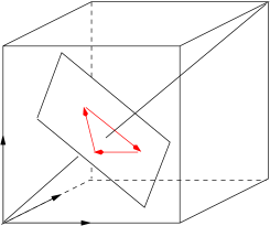
Figure 1: Projection of the position of the directed polymer onto the plane perpendicular to the $(1,1,1)$ direction (left) and directions for the 2D height function (right).

The projected height vector at level $k$, which is the generalized height function we are after, is then given by

$$\vec{H}^{\bot}_{k}=\vec{H}^{\bot}_{0}+\sum_{j=1}^{k}\left(n_{k}^{\Phi}\vec{\Phi}+n_{k}^{A}\vec{A}+n_{k}^{B}\vec{B}\right)$$ (4)

where $\vec{H}^{\bot}_{0}$ is the reference point (taken to be the origin in the description above). This shows that the local occupation numbers give the (discrete) height gradient

$$\nabla_{(111)}\vec{H}^{\bot}_{k}:=\vec{H}^{\bot}_{k}-\vec{H}^{\bot}_{k-1}=n_{k}^{\Phi}\vec{\Phi}+n_{k}^{A}\vec{A}+n_{k}^{B}\vec{B}$$ (5)

in $(111)$-direction. Fluctuations in the height vector are described by nearest neighbour particle swaps as defined above.

Correspondingly the surface path in the plane perpendicular to the $(111)$ direction becomes a planar random path on a honeycomb lattice with unit lattice constant (Fig. 2). A change in the path happens when two particles interchange places.

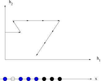
Figure 2: Two-dimensional random path on the honeycomb lattice and diffusing particles. From the left picture to the right picture, the black particle on lattice site 5 and the blue particle on lattice site 6 have interchanged places and the path has changed accordingly.

3 Coarse-grained dynamics and stationary spatio-temporal fluctuations

3.1 Coupled KPZ equations for the height function

In order to study the large-scale behaviour of the height function for arbitrary initial states we define a coarse-grained two-dimensional height variable

$$\vec{h}(x,t)=\left(\begin{matrix}h_{1}(x,t)\\ h_{2}(x,t)\end{matrix}\right).$$ (6)

Since $\vec{A}+\vec{B}+\vec{\Phi}=0$, it follows that $\rho_{A}=\rho_{B}=\rho_{\Phi}=1/3$ for the average particle densities. Therefore we define coarse-grained local densities $\rho_{A}(x,t),\rho_{B}(x,t)$ and $\rho_{\Phi}(x,t)$ for species $A,B$ and $\Phi$, respectively, as follows:

$$\rho_{A}(x,t) = \frac{1}{3}+\frac{2}{3}\;(\vec{A}\cdot\nabla\vec{h}(x,t))$$

$$\rho_{B}(x,t) = \frac{1}{3}+\frac{2}{3}\;(\vec{B}\cdot\nabla\vec{h}(x,t))$$

$$\rho_{\Phi}(x,t) = \frac{1}{3}+\frac{2}{3}\;(\vec{\Phi}\cdot\nabla\vec{h}(x,t))$$ (7)

Here, $\nabla\vec{h}$ denotes the one-dimensional derivative in the direction of the diffusing particles, i.e., along the coarse-grained chain in $(111)$-direction. Each of the densities fluctuates around its equilibrium value $\frac{1}{3}$ and will be changed proportionally to the change $\nabla\vec{h}$ in the height variable $\vec{h}(x,t)$ projected onto the respective growth direction.

In order to derive a nonlinear evolution equation for $\vec{h}(x,t)$ we recall that the local particle density describes the gradient of the height vector, see (5) for the discrete case. In order to obtain an equivalent continuum description we symmetrize the discrete gradient and expand the $\rho_{i}$ for $i=A,B,\Phi$ around $x$ to second order, leading to

$$\rho_{A}(x\pm\frac{1}{2})\simeq\frac{1}{3}+\frac{2}{3}\;(\vec{A}\cdot\nabla\vec{h})\mp\frac{1}{3}(\vec{A}\cdot\Delta\vec{h})+\cdots$$ (8)

The next step is to consider the time evolution of the height variable $\vec{h}(x,t)$. From the absence of correlations in the stationary distribution and the dynamical rules of the model we find

$$\dot{\vec{h}}(x) = (r_{3}-r_{4})(\vec{\Phi}-\vec{A})\;\rho_{\Phi}(x-\frac{1}{2})\;\rho_{A}(x+\frac{1}{2})$$ (9)

$$+(r_{1}-r_{2})(\vec{B}-\vec{A})\;\rho_{B}(x-\frac{1}{2})\;\rho_{A}(x+\frac{1}{2})$$

$$+(r_{5}-r_{6})(\vec{\Phi}-\vec{B})\;\rho_{\Phi}(x-\frac{1}{2})\;\rho_{B}(x+\frac{1}{2}).$$

This equation describes how the height variable will change after two particles on the lattice will have interchanged places. The increase is proportional to the density of particles and is proportional to the growth direction associated with the interchange process.

We will adopt the following notation:

$$r_{1}+r_{2} = p$$ (10)

$$r_{5}+r_{6} = q$$ (11)

$$r_{3}-r_{4} = f_{1}$$ (12)

$$r_{5}-r_{6} = f_{2}$$ (13)

$$r_{1}-r_{2} = f_{1}-f_{2}$$ (14)

The last equation follows from the pairwise balance requirement Eq.  (2). Putting everything into Eq. (9) and denoting transposition of a vector or matrix by a superscript $T$, we obtain

$$\frac{\partial}{\partial t}\vec{h}(x) = \left(\begin{matrix}\frac{1}{6}(f_{1}-2f_{2})\\ \frac{1}{2\sqrt{3}}f_{1}\end{matrix}\right)+\left(\begin{matrix}\frac{(f_{1}-2f_{2})}{6}&-\frac{f_{1}}{2\sqrt{3}}\\ -\frac{f_{1}}{2\sqrt{3}}&-\frac{(f_{1}-2f_{2})}{6}\end{matrix}\right)\nabla\vec{h}$$ (15)

$$+\left(\begin{matrix}\frac{(p+q)}{4}&\frac{(p-q)}{4\sqrt{3}}\\ \frac{(p-q)}{4\sqrt{3}}&\frac{2r_{1}+2r_{5}+3(p+q)}{12}\end{matrix}\right)\nabla^{2}\vec{h}$$

$$+\left(\begin{matrix}(\nabla\vec{h})^{T}\left(\begin{matrix}-\frac{(f_{1}-2f_{2})}{3}&-\frac{f_{1}}{2\sqrt{3}}\\ -\frac{f_{1}}{2\sqrt{3}}&0\end{matrix}\right)\nabla\vec{h}\\ (\nabla\vec{h})^{T}\left(\begin{matrix}0&-\frac{(f_{1}-2f_{2})}{6}\\ -\frac{(f_{1}-2f_{2})}{6}&-\frac{f_{1}}{\sqrt{3}}\end{matrix}\right)\nabla\vec{h}\end{matrix}\right)+\cdots$$

Taking the gradient on both sides one recognizes two coupled KPZ equations with non-vanishing drift term which mixes the two height components.

We express this system of non-linear coupled equations in terms of eigenfunctions of matrix multiplying $\nabla\vec{h}$. The eigenvalues are

$$v_{1,2}=\pm\frac{1}{3}\sqrt{f_{1}^{2}-f_{1}f_{2}+f_{2}^{2}}=:\pm\frac{1}{3}s(f_{1},f_{2}).$$ (16)

The expression under the square root is always positive except for $f_{1}=f_{2}=0$ in which case not only $v_{1}=v_{2}=0$ but where also the non-linear term vanishes. This corresponds to the (boring) case of symmetric diffusion which we exclude from our considerations. It is interesting that the two eigenvalues $\lambda_{1,2}$ are then never equal. This implies that the drift term cannot be removed by a Galilei transformation.

When $f_{1}=0$ we do not need to apply a similarity transformation. The result of the transformation to eigenmodes $\vec{\tilde{h}}(x)$ for $f_{1}\neq 0$ is

$$\frac{\partial}{\partial t}\vec{\tilde{h}}(x) = \left(\begin{matrix}\tilde{v}_{1}\\ \tilde{v}_{2}\end{matrix}\right)+\left(\begin{matrix}-\frac{1}{3}s(f_{1},f_{2})&0\\ 0&\frac{1}{3}s(f_{1},f_{2})\end{matrix}\right)\nabla\vec{\tilde{h}}(x)$$ (17)

$$+\left(\begin{matrix}M_{11}&M_{12}\\ M_{21}&M_{22}\end{matrix}\right)\nabla^{2}\vec{\tilde{h}}(x)+\left(\begin{matrix}(\nabla\vec{\tilde{h}}(x))^{T}\left(\begin{matrix}N_{11}&N_{12}\\ N_{21}&0\end{matrix}\right)\nabla\vec{\tilde{h}}(x)\\ (\nabla\vec{\tilde{h}}(x))^{T}\left(\begin{matrix}0&P_{12}\\ P_{21}&P_{22}\end{matrix}\right)\nabla\vec{\tilde{h}}(x)\end{matrix}\right)+\cdots$$

with the average growth velocities

$$\tilde{v}_{1} = \frac{f_{1}(f_{1}-2f_{2}+s(f_{1},f_{2}))(2f_{1}^{2}+2f_{2}(f_{2}+s(f_{1},f_{2}))-f_{1}(2f_{2}+s(f_{1},f_{2}))}{6s(f_{1},f_{2})|f_{1}|}$$

$$\tilde{v}_{2} = \frac{f_{1}(-f_{1}+2f_{2}+s(f_{1},f_{2}))(2f_{1}^{2}+2f_{2}(f_{2}-s(f_{1},f_{2}))+f_{1}(-2f_{2}+s(f_{1},f_{2}))}{6s(f_{1},f_{2})|f_{1}|}$$

of the two projected height variables in normal mode coordinates and the matrix elements

$$M_{11} = \frac{f_{2}(3(p-q)-(r_{1}+r_{5}))+(f_{1}-f_{2})(3(p-q)+r_{1}+r_{5})+2s(f_{1},f_{2})(3(p+q)+r_{1}+r_{5})}{24s(f_{1},f_{2})}$$

$$M_{22} = \frac{-f_{2}(3(p-q)+r_{1}+r_{5})-(f_{1}-f_{2})(3(p-q)+r_{1}+r_{5})+2s(f_{1},f_{2})(3(p+q)+r_{1}+r_{5})}{24s(f_{1},f_{2})}$$

$$M_{12} = -\frac{(-f_{1}+2f_{2}+2s(f_{1},f_{2}))\sqrt{6f_{1}^{2}-6f_{1}f_{2}+f_{2}(2f_{2}-s(f_{1},f_{2}))}}{24f_{1}s(f_{1},f_{2})\sqrt{6f_{1}^{2}-6f_{1}f_{2}+f_{2}(2f_{2}+s(f_{1},f_{2}))}}\times$$

$$\times(-2f_{1}(r_{1}+r_{5})+f_{2}(-p+q+(r_{1}+r_{5})))$$

$$M_{21} = -\frac{(f_{1}-2f_{2}+2s(f_{1},f_{2}))\sqrt{6f_{1}^{2}-6f_{1}f_{2}+f_{2}(2f_{2}+s(f_{1},f_{2}))}}{24f_{1}s(f_{1},f_{2})\sqrt{6f_{1}^{2}-6f_{1}f_{2}+f_{2}(2f_{2}-s(f_{1},f_{2}))}}\times$$

$$\times(-2f_{1}(r_{1}+r_{5})+f_{2}(-p+q+(r_{1}+r_{5})))$$

$$N_{11} = -\frac{f_{1}(f_{1}-2f_{2}+s(f_{1},f_{2}))\sqrt{6f_{1}^{2}-6f_{1}f_{2}+f_{2}(2f_{2}+s(f_{1},f_{2}))}}{3s(f_{1},f_{2})|f_{1}|}$$

$$P_{22} = -\frac{f_{1}(-f_{1}+2f_{2}+s(f_{1},f_{2}))\sqrt{6f_{1}^{2}-6f_{1}f_{2}+f_{2}(2f_{2}-s(f_{1},f_{2}))}}{3s(f_{1},f_{2})|f_{1}|}$$

$$N_{12} = N_{21}=-\frac{|f_{1}|((f_{1}-f_{2})(-(f_{1}-f_{2})^{2}+5(f_{1}-f_{2})s(f_{1},f_{2}))+f_{1}^{2}(-f_{1}+s(f_{1},f_{2})))}{6s(f_{1},f_{2})(f_{1})\sqrt{6f_{1}^{2}-6f_{1}f_{2}+f_{2}(2f_{2}-s(f_{1},f_{2}))}}$$

$$P_{12} = P_{21}=-\frac{|f_{1}|((f_{1}-f_{2})((f_{1}-f_{2})^{2}+5(f_{1}-f_{2})s(f_{1},f_{2}))+f_{1}^{2}(f_{1}+s(f_{1},f_{2})))}{6s(f_{1},f_{2})(f_{1})\sqrt{6f_{1}^{2}-6f_{1}f_{2}+f_{2}(2f_{2}+s(f_{1},f_{2}))}}$$

of the phenomenological diffusion matrix. The matrices $N$ and $P$ are the mode coupling matrices which yield the structure of the non-linear part of the coarse-grained evolution equation. We checked that for $f_{1}\neq 0$ the expressions under the square roots will always be positive or zero, and that the denominators are not zero. By rewriting these equations in terms of the height gradients $\vec{\tilde{\rho}}(x,t)=\nabla\vec{\tilde{h}}(x,t)$ one gets a system of coupled Burgers equations.

3.2 Stationary space-time fluctuations

As has become clear from the previous section it is convenient to work with height gradients which map to densities $\rho_{\alpha}(x,t)$ which are globally conserved, i.e., $\int\mathrm{d}x\rho_{\alpha}(x,t)=L\rho_{\alpha}$ for a system of length $L$. A fundamental quantity of interest is the dynamical structure function which are the stationary two-time correlations of the height gradients. For $n$ conserved densities this is an $n\times n$ matrix with the two-point correlations between the (centered) densities $u_{\alpha}(x,t)=\rho_{\alpha}(x,t)-\rho_{\alpha}$ at time $t_{0}$ and $t_{0}+t$. Because of stationarity $t_{0}$ is immaterial and can be set to 0.

3.2.1 Nonlinear fluctuating hydrodynamics

In order to study such a system with noisy dynamics on a coarse-grained level we follow the powerful and nonlinear fluctuating hydrodynamics (NLFH) approach [13] whose essence and main insights we briefly summarize.

Consider a system with $n$ conserved densities $\rho_{\alpha}$ and associated locally conserved currents $j_{\alpha}$. On coarse-grained Eulerian scale, where the noise drops out as a result of the law of large numbers, the conservation laws imply that the densities satisfy the nonlinear system of PDE’s [9, 20]

$$\frac{\partial}{\partial t}\vec{\rho}(x,t)+\frac{\partial}{\partial x}\vec{j}(x,t)=0$$ (18)

where component $\rho_{\alpha}(x,t)$ of the vector $\vec{\rho}(x,t)$ is a coarse-grained conserved quantity and the component $j_{\alpha}(x,t)$ of the current vector $\vec{j}(x,t)$ is the associated locally conserved current. Notice that in our convention $\vec{\rho}$ and $\vec{j}$ are regarded as column vectors.

Because of local stationarity under Eulerian scaling the current is a function of $x$ and $t$ only through its dependence on the local conserved densities. Hence these equations can be rewritten as

$$\frac{\partial}{\partial t}\vec{\rho}(x,t)+J(x,t)\frac{\partial}{\partial x}\vec{\rho}(x,t)=0$$ (19)

where $J(x,t)$ is the current Jacobian with matrix elements $J_{\alpha\beta}=\partial j_{\alpha}/\partial\rho_{\beta}$, understood as functions of $x$ and $t$ via $\rho_{\alpha}(x,t)$ via the stationary current-density relation $\vec{j}^{\ast}(\vec{\rho})$. In other words, $\vec{j}(x,t)=\vec{j}^{\ast}(\vec{\rho}(x,t))$. Obviously, constant densities $\rho_{\alpha}$ are a (trivial) stationary solution of (19). Stationary fluctuations of the conserved quantities are captured in the compressibility matrix $K$ that we shall not describe explicitly.

Up to this point the system (19), and therefore also its expansion in $u_{\alpha}(x,t)$, is completely deterministic. In the NLFH approach the effect of fluctuations is captured by adding a phenomenological diffusion matrix $D$ and white noise terms $\xi_{i}$. This turns (19) into a system of non-linear stochastic PDE’s. From renormalization group considerations it is known that polynomial non-linearities of order higher than 4 are irrelevant for the large-scale behaviour and order 3 leads at most to logarithmic corrections if the generic quadratic non-linearity is absent [21]. This justifies an expansion to second order so that the fluctuation fields $u_{\alpha}(x,t)$ satisfy the system of coupled noisy Burgers equations

$$\partial_{t}\vec{u}=-\partial_{x}\left(J\vec{u}+\frac{1}{2}\vec{u}^{T}\vec{H}\vec{u}-D\partial_{x}\vec{u}+B\vec{\xi}\right)$$ (20)

where $\vec{H}$ is a column vector whose entries $(\vec{H})_{\alpha}=H^{\alpha}$ are the Hessians with matrix elements $H^{\alpha}_{\beta\nu}=\partial^{2}j_{\alpha}/(\partial\rho_{\beta}\partial\rho_{\nu})$. If the quadratic non-linearity is absent one has diffusive behaviour. We stress that the Hessians $\vec{H}$ depend on the stationary densities around which one expands, but not on space and time. Hence they are fixed by the stationary current-density relation $\vec{j}^{\ast}(\vec{\rho})$.

In order to proceed further it is convenient to transform into normal modes $\vec{\phi}=R\vec{u}$ where $RJR^{-1}=\mathrm{diag}(v_{\alpha})$ and the transformation matrix $R$. The eigenvalues $v_{\alpha}$ of $J$ play the role of characteristic speeds that on microscopic scale describe the speed of local perturbations [22]. One thus arrives at

$$\partial_{t}\phi_{\alpha}=-\partial_{x}\left(v_{\alpha}\phi_{\alpha}+\vec{\phi}^{T}G^{\alpha}\vec{\phi}-\partial_{x}(\tilde{D}\vec{\phi})_{\alpha}+(\tilde{B}\vec{\xi})_{\alpha}\right)$$ (21)

with $\tilde{D}=RDR^{-1}$ and $\tilde{B}=RB$. The matrices

$$G^{\alpha}=\frac{1}{2}\sum_{\gamma}R_{\alpha\gamma}(R^{-1})^{T}H^{\gamma}R^{-1}$$ (22)

are the mode coupling matrices with the mode-coupling coefficients $G^{\alpha}_{\beta\gamma}=G^{\alpha}_{\gamma\beta}$ which are, by construction, symmetric. They are said to satisfy the trilinear condition if they satisfy also the symmetry $G^{\alpha}_{\beta\gamma}=G^{\beta}_{\alpha\gamma}$ [14, 15].

The main quantities of interest are then dynamical structure functions

$$S^{\alpha\beta}(x,t)=\mbox{$\langle\,{\phi^{\alpha}(x,t)\phi^{\beta}(0,0)}\,\rangle$}$$ (23)

which describe the stationary space-time fluctuations of the normal modes. They satisfy the normalization

$$\int_{-\infty}^{\infty}\mathrm{d}x\,S^{\alpha\beta}(x,t)=\delta_{\alpha,\beta}$$ (24)

which arises from the conservation law and the normalization condition $RKR^{T}=\mathds{1}$. It is important to note that in the absence of long-range order and long-range jumps generally the product $JK$ of the Jacobian with the compressibility matrix $K$ is symmetric, which can be proved mathematically rigorously [23]. This guarantees that on macroscopic scale the full non-linear system (19) is hyperbolic [24], i.e., characteristic velocities $v_{\alpha}$ are real.

When the characteristic velocities are all different, i.e., in the strictly hyperbolic case, the off-diagonal terms $S^{\alpha\beta}$ decay quickly and for long times and large distances one is left with the diagonal elements $S^{\alpha\alpha}(x,t)$ which are asymptotically universal functions $S^{\alpha\alpha}(x,t)\sim t^{-1/z_{\alpha}}f(u_{\alpha})$ with the scaling variable $u_{\alpha}=(x-v_{\alpha}t)^{z_{\alpha}}/t$. Here $z_{\alpha}$ is the dynamical exponent.

These scaling functions can be evaluated using mode coupling theory [13, 25]. As pointed out in the introduction, in systems with short-range interactions there is an infinite discrete family of universality classes with dynamical exponents $z_{\alpha}$ that are the Kepler ratios of neighbouring Fibonacci numbers $F_{\alpha+2}/F_{\alpha+1}$ [4], beginning with $z_{1}=2=F_{3}/F_{2}$ corresponding to diffusion and Gaussian scaling function $f$, followed by $z_{\alpha}=3/2,5/3,8/5,\dots$. Also the limit value of this sequence, which is the golden mean $\phi=(1+\sqrt{5})/2$, can arise.

Which dynamical universality classes appear depends on which diagonal elements of the mode coupling matrix vanish. A full classification for $n=2$ is given in [3, 7] and for general $n$ in [25]. For $n=2$ one can have diffusion with $z=2$, and also exponents $z=3/2,5/3,\phi$. The dynamical exponent $z=3/2$ can describe the KPZ universality class [2] (in which case the scaling function $f$ is the celebrated Prähofer-Spohn function [26]), or a modified KPZ universality class with unknown scaling function [3], or a Lévy universality class [3, 5, 25, 27]. The $z=5/3$ Lévy class characterizes the heat mode in anharmonic chains [28, 29] and one-dimensional fluids obeying Hamiltonian dynamics [6]. Experimental evidence for anomalous heat conduction has been found in single multiwalled carbon and boron-nitride nanotubes at room temperature [33].

The upshot of the mode coupling treatment of NLFH is that the dynamical universality classes can be directly inferred from the structure of the mode coupling matrices, which in turn is fully determined by the stationary current-density relation $\vec{j}^{\ast}(\vec{\rho})$ for the conserved densities $\vec{\rho}$ of the system.

The theory of non-linear fluctuating hydrodynamics combined with mode-coupling theory is rather robust. It relies fundamentally on the presence long-lived long wave-length modes which arise from the conservation laws. Excluded are (i) systems that exhibit long-range order in the stationary state, in which case complex characteristic velocities indicative of phase separation [34, 35] may arise. (ii) In systems with long-range interactions other discrete dynamical exponents may appear, e.g., the ballistic universality class with $z=1$ in nearest-neighbour hopping with long-range dependence of the hopping rate [36, 37, 38], or in models with long-range jumps such as the Oslo rice pile model with $z=10/7$ [39] or the raise-and-peel model [40], also with $z=1$. (iii) Also integrable models with non-local conservation laws might conceivably exhibit dynamical exponents that are not Kepler ratios. However, so far there is no evidence for such an anomaly [41].

The family of height models considered here falls into neither of these three long-range categories (i) – (iii) and therefore one expects all dynamical exponents to be the Kepler ratios derived in [4]. They appear in combinations that can be derived from the mode coupling matrices for a general number of conservation laws following [25] and specifically for $n=2$ from the earlier work [3, 7]. In the following we compute the mode coupling matrices for the directed polymer model first for $n=2$ (corresponding to $d=3$) and then for general $n$ in order to work out the dynamical universality classes of the $n$ generalized height functions.

3.2.2 Fluctuations in $d=3$

In the following we apply the approach based on NLFH that we have outlined above to the directed polymer model in three dimensions, with the aim of identifying its universal classes through analysis of the mode-coupling matrix.

When $f_{1}=0$ the matrices appearing in the quadratic term in the r.h.s. of (15) are the mode coupling matrices (22) introduced above. One sees that the height variable $h_{2}$ has neither a quadratic self-coupling nor a non-linear coupling to $h_{1}$. On the other hand, $h_{1}$ has a non-vanishing quadratic non-linearity, but no quadratic coupling to the diffusive mode. Hence according to [3, 7] the evolution of $h_{2}$ is diffusive and mode 1 is KPZ.

In the matrices $N$ and $P$ one recognizes the mode coupling matrices $G^{\alpha}$ (22) arising from NLFH. Thus the universality classes can be identified. Since both mode coupling matrices have generically non-vanishing self-coupling coefficients $N_{11}$ and $P_{22}$ we arrive at the conclusion that generically the two-component height model has two KPZ modes drifting away from each other with speeds (16). Similar models were studied by Kim and den Nijs [42] and Ferrari, Sasamoto and Spohn [14].

Notice, however, that $s(f,f)=s(f,0)=f$ Therefore when $f_{1}=f_{2}=:f\neq 0$ one has $s(f,f)=f$ and therefore $N_{11}=0$, $P_{22}\neq 0$. In this case mode 1 is diffusive while mode 2, which has no coupling to the diffusive mode, is KPZ. On the other hand, when $f_{1}=f\neq 0$ and $f_{2}=0$ one gets $N_{11}\neq 0$, $P_{22}=0$, which is the same scenario with the role of two modes interchanged. Therefore also mixed dynamics may occur. In the trivial case where $f_{1}=f_{2}=0$ both modes are diffusive.

4 The $n$-component particle exchange process

As discussed above the mapping between the height model and exclusion can be applied to any dimension $d\geq 2$. Here we define the corresponding multi-species exclusion process and discuss it in detail in the hopping rates for which the stationary distribution factorizes. We shall call this process the $n$-component particle exchange process (PEP). For more general exclusion processes with nearest-neighbour particle exchange and non-factorized stationary distributions we refer to [43, 44] and, for the present context, to [14]. We derive the exact mode coupling matrices in explicit form and thus identify the possible universality classes for arbitrary dimension $d$.

4.1 Definition and stationary properties

In the $n$-component PEP an exclusion particle of type $\alpha\in\{0,1,\dots,M\}$ on site $k$ exchanges with type $\beta$ on site $k+1$ with rate $g_{\alpha,\beta}$, symbolically

$$A_{\alpha}A_{\beta}\to A_{\beta}A_{\alpha}\quad\mbox{ with rate }g_{\alpha,\beta}.$$

Type 0 is called vacancy and we speak of $M$ distinct conserved species of particles. The total number of particles of each species in the system is denoted $N_{\alpha}$. We consider $L$ sites with periodic boundary conditions. It is convenient to decompose the rates into a symmetric part $w_{\alpha,\beta}=w_{\beta,\alpha}>0$ for $\alpha\neq\beta$ and an antisymmetric part $f_{\alpha,\beta}=-f_{\beta,\alpha}$ in the form

$$g_{\alpha,\beta}=\frac{1}{2}(w_{\alpha,\beta}+f_{\alpha,\beta}).$$ (25)

Positivity of the rates implies $w_{\alpha,\beta}\geq|f_{\alpha,\beta}|$. For convenience we define $w_{\alpha,\alpha}=f_{\alpha,\alpha}=0$ and denote the vacuum driving fields for particles with vacant neighbors by

$$f_{\alpha}:=f_{\alpha,0}$$ (26)

which implies, by definition, $f_{0}=0$. If for some $\alpha$ one has $w_{\alpha,0}=|f_{\alpha}|$, the vacuum motion of species $\alpha$ is totally asymmetric.

From pairwise balance [19] we find that the canonical stationary distribution with $N_{\alpha}$ particles is uniform, provided that the condition

$$f_{\alpha,\beta}=f_{\alpha}-f_{\beta}$$ (27)

is satisfied with driving fields in the physical domain $|f_{\alpha}|\leq w_{\alpha,0}$. It follows that the grandcanonical stationary ensemble with fluctuating particle numbers is a product measure defined by fugacities $\mu_{\alpha}$, or equivalently, particle densities

$$\rho_{\alpha}:=\mbox{$\langle\,{N_{\alpha}}\,\rangle$}/L=\frac{\mathrm{e}^{\mu_{\alpha}}}{\sum_{\alpha^{\prime}=0}^{M}\mathrm{e}^{\mu_{\alpha}^{\prime}}}$$ (28)

The product structure leads to the covariances (generalized compressibilities)

$$\kappa_{\alpha\beta}:=\frac{\partial\rho_{\alpha}}{\partial\mu_{\beta}}=1/L\mbox{$\langle\,{(N_{\alpha}-\mbox{$\langle\,{N_{\alpha}}\,\rangle$})(N_{\beta}-\mbox{$\langle\,{N_{\beta}}\,\rangle$})}\,\rangle$}=\rho_{\alpha}(\delta_{\alpha,\beta}-\rho_{\beta}).$$ (29)

We denote the compressibility matrix with matrix elements $\kappa_{\alpha\beta}$ by $K$. By construction $K=K^{T}$ is symmetric.

Consider the local density $\rho_{k}^{\alpha}:=\mbox{$\langle\,{n_{k}^{\alpha}}\,\rangle$}$, i.e., the expectation of the local particle number $n_{k}^{\alpha}\in\{0,1\}$. Particle number conservation implies the discrete continuity equation

$$\frac{d}{dt}\rho_{k}^{\alpha}=j_{k-1}^{\alpha}-j_{k}^{\alpha}$$ (30)

where, by definition of the process, the expected local current of species $\alpha$ is given by

$$j_{k}^{\alpha}=\sum_{\beta=0}^{M}g_{\alpha,\beta}\mbox{$\langle\,{n_{k}^{\alpha}n_{k+1}^{\beta}}\,\rangle$}-g_{\beta,\alpha}\mbox{$\langle\,{n_{k}^{\beta}n_{k+1}^{\alpha}}\,\rangle$}.$$ (31)

In the grandcanonical stationary distribution one has

$$j_{\alpha}=\rho_{\alpha}\left(f_{\alpha}-\sum_{\beta=1}^{M}f_{\beta}\rho_{\beta}\right).$$ (32)

This follows from the factorization property of the grandcanonical stationary distribution.

4.2 Collective velocities

As dicussed above one expects in the hydrodynamic limit on Euler scale the system of conservation laws (19) where $J$ is the flux Jacobian with matrix elements

$$J_{\alpha\beta}=\frac{\partial j_{\alpha}}{\partial\rho_{\beta}}=\left[f_{\alpha}-\sum_{\gamma=1}^{M}f_{\gamma}\rho_{\gamma}\right]\delta_{\alpha,\beta}-f_{\beta}\rho_{\alpha}$$ (33)

In order to derive the normal modes for non-zero densities and non-zero driving fields we introduce the diagonal matrices $\hat{\rho}:=\mathrm{diag}(\rho_{\alpha})$ and $\hat{f}:=\mathrm{diag}(f_{\alpha})$ with the densities and driving fields resp. on the diagonal. Then we can write

$$J=D^{-1}BD$$ (34)

where $D=\sqrt{\hat{f}/\hat{\rho}}$ and $B=B^{T}$. The non-diagonal matrix elements of $B$ are $B_{\alpha\beta}=-\sqrt{f_{\alpha}\rho_{\alpha}f_{\beta}\rho_{\beta}}$. This implies that $J$ can be diagonalized with the help of $D$ and an orthgonal matrix $\mathcal{O}$. With $\hat{J}:=\mathrm{diag}(v_{i})$ one can write

$$RJR^{-1}=\hat{J}$$ (35)

where $R=Q^{-1}\mathcal{O}D$ and $R^{-1}=D^{-1}\mathcal{O}^{T}Q$ with an invertible diagonal matrix $Q=\mathrm{diag}(q_{\alpha})$. Notice also that $R^{T}=D\mathcal{O}^{T}Q^{-1}$ and $(R^{-1})^{T}=Q\mathcal{O}D^{-1}$. Choosing $Q$ such that

$$RKR^{T}=\mathds{1}$$ (36)

one obtains an orthonormal basis of the modes. To compute the matrix $Q$ we observe that

$$J=KD^{2}-\sum_{\alpha}f_{\alpha}\rho_{\alpha}\mathds{1}.$$ (37)

Thus $RKR^{T}=Q^{-1}\mathcal{O}DJD^{-1}\mathcal{O}^{T}Q^{-1}+\sum_{\alpha}f_{\alpha}\rho_{\alpha}Q^{-1}\mathcal{O}\mathcal{O}^{T}Q^{-1}=(RAR^{-1}+\sum_{\alpha}f_{\alpha}\rho_{\alpha}\mathds{1})Q^{-2}$. This yields

$$q_{\alpha}^{2}=v_{\alpha}+\sum_{\alpha}f_{\alpha}\rho_{\alpha}.$$ (38)

We remark that decomposing $J$ into a traceless part and the trace yields

$$J=\tilde{J}+\frac{1}{M}\sum_{\alpha}f_{\alpha}\left(1-(M+1)\rho_{\alpha}\right)\mathds{1}$$ (39)

which can be written in the form $J=D^{-1}\tilde{B}D+V\mathds{1}$ with traceless and symmetric $\tilde{B}$. For the completely symmetric state with $\rho_{\alpha}=1/(M+1)$ as for the generalized height model one has $V=0$ and the collective velocities are the eigenvalues of $\tilde{B}$. On the other hand, for equal driving fields $f_{\alpha}=f$ one has $V=f(1-\sum_{\alpha=1}^{M}\rho_{\alpha})$ which vanishes only for the completely filled lattice. This then is the multispecies simple exclusion process.

4.3 Mode-coupling coefficients

The Hessians

$$H^{\gamma}_{\alpha\beta}:=\frac{\partial^{2}j^{\gamma}}{\partial\rho_{\alpha}\partial\rho_{\beta}}=\partial_{\alpha}J_{\gamma\beta}$$ (40)

are constants

$$H^{\gamma}_{\alpha\beta}=-\left(f_{\alpha}\delta_{\beta,\gamma}+f_{\beta}\delta_{\alpha,\gamma}\right).$$ (41)

This simple form allows us to compute explicitly the mode-coupling coefficients

$$G^{\gamma}_{\alpha\beta}:=\frac{1}{2}\sum_{\lambda}R_{\gamma\lambda}\left[(R^{-1})^{T}H^{\lambda}R^{-1}\right]_{\alpha\beta}.$$ (42)

According to the definitions given above we have

$$D_{\alpha\beta}=\sqrt{\frac{f_{\alpha}}{\rho_{\alpha}}}\delta_{\alpha,\beta}$$ (43)

and

$$R_{\alpha\beta}=q_{\alpha}^{-1}\sqrt{\frac{f_{\beta}}{\rho_{\beta}}}\mathcal{O}_{\alpha\beta}, (R^{-1})_{\alpha\beta}=q_{\beta}\sqrt{\frac{\rho_{\alpha}}{f_{\alpha}}}\mathcal{O}_{\beta\alpha}=q^{2}_{\beta}\frac{\rho_{\alpha}}{f_{\alpha}}(R^{T})_{\alpha\beta},$$

$$(R^{T})_{\alpha\beta}=q_{\beta}^{-1}\sqrt{\frac{f_{\alpha}}{\rho_{\alpha}}}\mathcal{O}_{\beta\alpha}, ((R^{-1})^{T})_{\alpha\beta}=q_{\alpha}\sqrt{\frac{\rho_{\beta}}{f_{\beta}}}\mathcal{O}_{\alpha\beta}=q^{2}_{\alpha}\frac{\rho_{\beta}}{f_{\beta}}R_{\alpha\beta}.$$ (44)

Hence, by straightforward computation

$$G^{\gamma}_{\alpha\beta} = \frac{1}{2}\sum_{\lambda}\sum_{\mu}\sum_{\nu}R_{\gamma\lambda}((R^{-1})^{T})_{\alpha\mu}H^{\lambda}_{\mu\nu}(R^{-1})_{\nu\beta}$$

$$= -\frac{1}{2}\sum_{\mu}\sum_{\nu}\left[f_{\mu}R_{\gamma\nu}((R^{-1})^{T})_{\alpha\mu}(R^{-1})_{\nu\beta}+f_{\nu}R_{\gamma\mu}((R^{-1})^{T})_{\alpha\mu}(R^{-1})_{\nu\beta}\right]$$

$$= -\frac{1}{2}\sum_{\mu}\left[f_{\mu}\,((R^{-1})^{T})_{\alpha\mu}\,\delta_{\beta,\gamma}+f_{\mu}\,(R^{-1})_{\mu\beta}\,\delta_{\alpha,\gamma}\right]$$

$$= -\frac{1}{2}\left[q^{2}_{\alpha}\sum_{\mu}R_{\alpha\mu}\rho_{\mu}\,\delta_{\beta,\gamma}+q^{2}_{\beta}\sum_{\mu}R_{\beta\mu}\rho_{\mu}\,\delta_{\alpha,\gamma}\right]$$

$$= -\frac{1}{2}\left[q^{2}_{\alpha}(R\vec{\rho})_{\alpha}\,\delta_{\beta,\gamma}+q^{2}_{\beta}(R\vec{\rho})_{\beta}\,\delta_{\alpha,\gamma}\right].$$

We point out the non-trivial trilinear property $G^{\gamma}_{\alpha\beta}=G^{\alpha}_{\gamma\beta}$ which one expects for systems where the driving force does not change the stationary distribution [14, 15].

For the diagonal elements one has

$$G^{\gamma}_{\alpha\alpha}=-q^{2}_{\alpha}\,(R\vec{\rho})_{\alpha}\,\delta_{\alpha,\gamma}.$$ (46)

Hence generically all modes are KPZ and there are only subleading corrections since $G^{\gamma}_{\alpha\alpha}=0$ for $\alpha\neq\gamma$. If one of the coefficients $q^{2}_{\alpha}(R\vec{\rho})_{\alpha}$ vanishes, then this mode is diffusive and all other modes evolve independently of this mode.

4.4 Details for two conservation laws

We return to the case $n=2$ and at least one driving field non-zero and present the diagonalization explicitly and in detail for arbitrary densities. For the two-component PEP with arbitrary densities $\rho_{\alpha}$ we have

$$j_{1}=f_{1}\rho_{1}(1-\rho_{1})-f_{2}\rho_{1}\rho_{2},\quad j_{2}=f_{2}\rho_{2}(1-\rho_{2})-f_{1}\rho_{1}\rho_{2}$$ (47)

and the compressibility matrix is given by

$$K=\left(\begin{array}[]{cc}\rho_{1}(1-\rho_{1})&-\rho_{1}\rho_{2}\\ -\rho_{1}\rho_{2}&\rho_{2}(1-\rho_{2})\end{array}\right).$$ (48)

We find

$$J = \left(\begin{array}[]{cc}f_{1}(1-2\rho_{1})-f_{2}\rho_{2}&-f_{2}\rho_{1}\\ -f_{1}\rho_{2}&f_{2}(1-2\rho_{2})-f_{1}\rho_{1}\end{array}\right)$$ (51)

$$= \left(\begin{array}[]{cc}\frac{1}{2}(f_{1}(1-\rho_{1})-f_{2}(1-\rho_{2}))&-f_{2}\rho_{1}\\ -f_{1}\rho_{2}&-\frac{1}{2}(f_{1}(1-\rho_{1})-f_{2}(1-\rho_{2}))\end{array}\right)$$

$$+\frac{1}{2}\sum_{\alpha=1}^{2}f_{\alpha}(1-3\rho_{\alpha})\mathds{1}.$$

In order to compute the eigenvalues of $J$ we use (39). For $n=2$ this yields as eigenvalues of $\tilde{B}$ the quantities $\pm\sqrt{\det{\tilde{B}}}$ and therefore

$$v_{1,2}=\frac{1}{2}\left[\sum_{\alpha=1}^{2}f_{\alpha}\left(1-3\rho_{\alpha}\right)\pm\sqrt{[f_{1}(1-\rho_{1})-f_{2}(1-\rho_{2})]^{2}+4f_{1}\rho_{1}f_{2}\rho_{2}}\right].$$ (55)

In the domain of interest $0<\rho_{1}+\rho_{2}<1$ one has $\det{\tilde{B}}>0$. Hence the corresponding system of conservation laws is strictly hyperbolic. For the special case $\rho_{1}=\rho_{3}=1/3$ we recover (16).

In order to compute $R$ we define the orthgonal matrix

$$\mathcal{O}=\left(\begin{array}[]{cc}\cos{\phi}&-\sin{\phi}\\ \sin{\phi}&\cos{\phi}\end{array}\right).$$ (56)

Straightforward computation shows that $J$ is diagonalized with the choice

$$\tan{(2\phi)}=\frac{2\sqrt{f_{1}\rho_{1}f_{2}\rho_{2}}}{f_{1}(1-\rho_{1})-f_{2}(1-\rho_{2})}.$$ (57)

This yields, together with (36),

$$R=\left(\begin{array}[]{cc}q_{1}^{-1}\sqrt{\frac{f_{1}}{\rho_{1}}}\cos{\phi}&-q_{1}^{-1}\sqrt{\frac{f_{2}}{\rho_{2}}}\sin{\phi}\\ q_{2}^{-1}\sqrt{\frac{f_{1}}{\rho_{1}}}\sin{\phi}&q_{2}^{-1}\sqrt{\frac{f_{2}}{\rho_{2}}}\cos{\phi}\end{array}\right),R^{-1}=\left(\begin{array}[]{cc}q_{1}\sqrt{\frac{\rho_{1}}{f_{1}}}\cos{\phi}&q_{2}\sqrt{\frac{\rho_{1}}{f_{1}}}\sin{\phi}\\ -q_{1}\sqrt{\frac{\rho_{2}}{f_{2}}}\sin{\phi}&q_{2}\sqrt{\frac{\rho_{2}}{f_{2}}}\cos{\phi}\end{array}\right)$$ (58)

where

$$q_{i}^{2}=v_{i}+f_{1}\rho_{1}+f_{2}\rho_{2}.$$ (59)

The Hessians are

$$H^{1}=-\left(\begin{array}[]{cc}2f_{1}&f_{2}\\ f_{2}&0\end{array}\right),\quad H^{2}=-\left(\begin{array}[]{cc}0&f_{1}\\ f_{1}&2f_{2}\end{array}\right)$$ (60)

and (42) yields

$$G^{1}=-\frac{1}{2}\left(\begin{array}[]{cc}2g_{1}&g_{2}\\ g_{2}&0\end{array}\right),\quad G^{2}=-\frac{1}{2}\left(\begin{array}[]{cc}0&g_{1}\\ g_{1}&2g_{2}\end{array}\right)$$ (61)

with coupling constants

$$g_{1}=q_{1}\left(\sqrt{f_{1}\rho_{1}}\cos{\phi}-\sqrt{f_{2}\rho_{2}}\sin{\phi}\right),\quad g_{2}=q_{2}\left(\sqrt{f_{1}\rho_{1}}\sin{\phi}-\sqrt{f_{2}\rho_{2}}\cos{\phi}\right).$$ (62)

As expected, generically both modes are KPZ with subleading corrections.

Care has to be taken if $f_{1}=0$ and $f_{2}=f\neq 0$. Then

$$j_{1}=-f\rho_{1}\rho_{2},\quad j_{2}=f\rho_{2}(1-\rho_{2})$$ (63)

and

$$J=\left(\begin{array}[]{cc}-f\rho_{2}&-f\rho_{1}\\ 0&f(1-2\rho_{2})\end{array}\right).$$ (64)

This yields the collective velocities

$$v_{1}=-f\rho_{2},\quad v_{2}=f(1-2\rho_{2})$$ (65)

and

$$R=\left(\begin{array}[]{cc}\sqrt{\frac{1-\rho_{2}}{\rho_{1}(1-\rho_{1}-\rho_{2})}}&\sqrt{\frac{\rho_{1}}{(1-\rho_{1}-\rho_{2})(1-\rho_{2})}}\\ 0&\frac{1}{\sqrt{\rho_{2}(1-\rho_{2})}}\end{array}\right),\quad R^{-1}=\left(\begin{array}[]{cc}\sqrt{\frac{\rho_{1}(1-\rho_{1}-\rho_{2})}{1-\rho_{2}}}&-\rho_{1}\sqrt{\frac{\rho_{2}}{1-\rho_{2}}}\\ 0&\sqrt{\rho_{2}(1-\rho_{2})}\end{array}\right).$$ (66)

For the Hessians one has

$$H^{1}=-f\left(\begin{array}[]{cc}0&1\\ 1&0\end{array}\right),\quad H^{2}=-2f\left(\begin{array}[]{cc}0&0\\ 0&1\end{array}\right).$$ (67)

Then (42) yields

$$G^{1}=-\frac{f}{2}\sqrt{\rho_{2}(1-\rho_{2})}\left(\begin{array}[]{cc}0&1\\ 1&0\end{array}\right),\quad G^{2}=-f\sqrt{\rho_{2}(1-\rho_{2})}\left(\begin{array}[]{cc}0&0\\ 0&1\end{array}\right).$$ (68)

(We remind the reader that the labels at $G$ and $H$ are upper indices, not powers). Hence mode 1 is diffusive and mode 2 is KPZ.

The case $f_{2}=0$ and $f_{1}=f\neq 0$ follows by symmetry. We also consider $f_{1}=f_{2}=f$. In this case (57) yields $\tan{\phi}=\sqrt{\rho_{1}/\rho_{2}}$ in which case (62) gives $g_{1}=0$, or $\tan{\phi}=-\sqrt{\rho_{2}/\rho_{1}}$ in which case $g_{2}=0$. Hence one of the modes is diffusive, as first argued in [45].

5 Conclusions

We have treated coupled non–linear stochastic PDE equations of KPZ type in two different contexts: A model for directed polymers in $d=3$ where we derived from a dynamical mean field approach a system of two coupled partial differential equations, and from non–linear fluctuating hydrodynamics theory where the same equations are shown to follow from conservation laws for the densities and the presence of noise. These equations can then be treated in mode coupling theory. Both approaches lead to the same structure of the mode coupling terms.

Next we generalized the lattice gas approach to an arbitrary number $n$ of conserved particle species, corresponding to a model for directed polymers in $d=n+1$ dimensions. Thus we give a direct physical link between fluctuations in the conformations of the polymer and the underlying particle exchange processes on the lattice. This allows in particular to understand and access different cases of the general classification given in [3, 7] for two conservation laws and for an arbitrary number of conservation laws in [4, 25]. It turns out that stationary spatio-temporal fluctuations in the polymer model are generally either diffusive or in the universality class of the one-dimensional KPZ equation.

There is an interesting open problem: The totally asymmetric two-component model ($w_{10}=f_{1}$, $w_{20}=f_{2}$ $w_{12}=f_{1}-f_{2}$) is integrable [46]. Can one use the integrability to obtain directly the exact scaling form of the dynamical structure function? From the results of the present work one expects this to be the Praehofer-Spohn scaling function [26] for each mode separately.

References

- [1] S. Lepri (ed.), Thermal Transport in Low Dimensions: From Statistical Physics to Nanoscale Heat Transfer, Lecture Notes in Physics 921, (Springer, Switzerland, 2016).
- [2] T. Halpin-Healy, K.A. Takeuchi, A KPZ Cocktail-Shaken, not Stirred…, J. Stat. Phys. 160(4), 794–814 (2015).
- [3] H. Spohn H and G. Stoltz, Nonlinear fluctuating hydrodynamics in one dimension: The case of two conserved fields, J. Stat. Phys. 160 861–884 (2015).
- [4] V. Popkov, A. Schadschneider, J. Schmidt, and G.M. Schütz, Fibonacci family of dynamical universality classes, Proc. Natl. Acad. Science (USA) 112(41) 12645–12650 (2015).
- [5] C. Bernardin, P. Gonçalves, and M. Jara, 3/4-fractional superdiffusion in a system of harmonic oscillators perturbed by a conservative noise, Arch. Rational Mech. Anal. 220, 505–542 (2016).
- [6] H. van Beijeren, Exact results for transport properties of one-dimensional hamiltonian systems, Phys. Rev. Lett. 108, 180601 (2012).
- [7] V. Popkov, J. Schmidt, and G.M. Schütz, Universality classes in two-component driven diffusive systems. J. Stat. Phys. 160, 835–860 (2015).
- [8] D. Ertaş and M. Kardar, Dynamic relaxation of drifting polymers: A phenomenological approach, Phys. Rev.E 48, 1228–1245 (1993).
- [9] H. Spohn, Large Scale Dynamics of Interacting Particles. (Springer, Berlin, 1991).
- [10] T. M. Liggett, Stochastic Interacting Systems: Contact, Voter and Exclusion Processes Springer, Berlin (1999).
- [11] G.M. Schütz, Exactly solvable models for many-body systems far from equilibrium, in: Phase Transitions and Critical Phenomena. Vol. 19, C. Domb and J. Lebowitz (eds.), Academic Press, London (2001).
- [12] A. Schadschneider, D. Chowdhury, K Nishinari. Stochastic Transport in Complex Systems. Elsevier, Amsterdam (2010).
- [13] H. Spohn, Nonlinear Fluctuating hydrodynamics for anharmonic chains, J. Stat. Phys. 154, 1191–1227 (2014).
- [14] P.L. Ferrari, T. Sasamoto and H. Spohn, Coupled Kardar-Parisi-Zhang equations in one dimension, J. Stat. Phys. 153, 377–399 (2013).
- [15] T. Funaki, Infinitesimal invariance for the coupled KPZ equations, Memoriam Marc Yor – Séminaire de Probabilités XLVII, Lect. Notes Math., 2137, 37–47, (Springer, Switzerland, 2015).
- [16] P. Meakin, P. Ramanlal, L.M. Sander and R.C. Ball, Ballistic deposition on surfaces, Phys. Rev. A 34, 5091–5103 (1986).
- [17] M Plischke, Z Ràcz, and D Liu, Time-reversal invariance and universality of two-dimensional growth models, Phys. Rev. B 35, 3485–3495 (1987).
- [18] G.M. Schütz, Critical phenomena and universal dynamics in one-dimensional driven diffusive systems with two species of particles, J. Phys. A 36, R339 - R379 (2003).
- [19] G.M. Schütz, R. Ramaswamy and M. Barma, Pairwise balance and invariant measures for generalized exclusion processes, J. Phys. A: Math. Gen. 29, 837–845 (1996).
- [20] C. Kipnis and C. Landim, Scaling limits of interacting particle systems in: Grundlehren der mathematischen Wissenschaften Vol. 320 (Springer, Berlin, 1999).
- [21] P. Devillard and H. Spohn, Universality class of interface growth with reflection symmetry. J. Stat. Phys. 66, 1089–1099 (1992).
- [22] V. Popkov and G.M. Schütz, Shocks and excitation dynamics in a driven diffusive two-channel system, J. Stat. Phys. 112, 523-540 (2003).
- [23] R. Grisi and G.M. Schütz, Current symmetries for particle systems with several conservation laws, J. Stat. Phys. 145, 1499–1512 (2011).
- [24] B. Tóth and B. Valkó, Onsager relations and Eulerian hydrodynamic limit for systems with several conservation laws, J. Stat. Phys. 112, 497–521 (2003).
- [25] V. Popkov, A. Schadschneider, J. Schmidt, G.M. Schütz, Exact scaling solution of the mode coupling equations for non-linear fluctuating hydrodynamics in one dimension, J. Stat. Mech. 093211 (2016).
- [26] M. Prähofer and H. Spohn, Exact scaling function for one-dimensional stationary KPZ growth, J. Stat. Phys. 115, 255–279 (2004).
- [27] V. Popkov, J. Schmidt, and G.M. Schütz, Superdiffusive modes in two-species driven diffusive systems. Phys. Rev. Lett. 112, 200602 (2014).
- [28] C.B. Mendl and H. Spohn, Dynamic correlators of FPU chains and nonlinear fluctuating hydrodynamics. Phys. Rev. Lett. 111, 230601 (2013).
- [29] D. Xiong, Underlying mechanisms for normal heat transport in one-dimensional anharmonic oscillator systems with a double-well interparticle interaction, J. Stat. Mech. 043208 (2016).
- [30] P. Cipriani, S. Denisov and A. Politi, From anomalous energy diffusion to Lévy walks and heat conductivity in one-dimensional systems, Phys. Rev. Lett. 94, 244301 (2005).
- [31] D. Xiong, J. Wang, Y. Zhang, and H. Zhao, Nonuniversal heat conduction of one-dimensional lattices, Phys. Rev. E 85, 020102 (2012).
- [32] P. L. Hurtado, and P. L. Garrido, A violation of universality in anomalous Fourier’s law, Sci. Rep. 6 38823 (2016).
- [33] C. W. Chang, D. Okawa, H. Garcia, A. Majumdar, and A. Zettl, Breakdown of Fourier’s Law in Nanotube Thermal Conductors, Phys. Rev. Lett. 101, 075903 (2008).
- [34] S. Ramaswamy, M. Barma, D. Das, and A. Basu, Phase Diagram of a Two-Species Lattice Model with a Linear Instability, Phase Transit. 75, 363–375 (2002).
- [35] S. Chakraborty, S. Pal, S. Chatterjee and M. Barma, Large compact clusters and fast dynamics in coupled nonequilibrium systems, Phys. Rev. E 93, 050102(R) (2016).
- [36] H. Spohn, Bosonization, vicinal surfaces, and hydrodynamic fluctuation theory, Phys. Rev. E 60, 6411–6420 (1999).
- [37] V. Popkov, D. Simon, and G.M. Schütz, ASEP on a ring conditioned on enhanced flux, J. Stat. Mech. P10007 (2010).
- [38] V. Popkov and G. M. Schütz, Transition probabilities and dynamic structure factor in the ASEP conditioned on strong flux, J. Stat. Phys. 142(3), 627–639 (2011).
- [39] P. Grassberger, D. Dhar, and P. K. Mohanty, Oslo model, hyperuniformity, and the quenched Edwards-Wilkinson model, Phys. Rev. E 94, 042314 (2016).
- [40] F.C. Alcaraz, and V. Rittenberg, Different facets of the raise and peel model, J. Stat. Mech. P07009 (2007).
- [41] A. Kundu, and A. Dhar, Equilibrium dynamical correlations in the Toda chain and other integrable models, Phys. Rev. E 94, 062130 (2016).
- [42] K.H. Kim and M. den Nijs, Dynamic screening in a two-species asymmetric exclusion process, Phys. Rev. E 76 021107 (2007).
- [43] A. P. Isaev, P. N. Pyatov and V. Rittenberg, Diffusion algebras, J. Phys. A: Math. Gen. 34, 5815–5834 (2001).
- [44] B. Aneva, Deformed coherent and squeezed states of multiparticle processes, Eur. Phys. J. C 31, 403–414 (2003).
- [45] A. Rákos and G.M. Schütz, Exact shock measures and steady state selection in a driven diffusive system with two conserved densities, J. Stat. Phys. 117, 55-76 (2004).
- [46] V. Popkov, E. Fouladvand and G.M. Schütz, A sufficient integrability criterion for interacting particle systems and quantum spin chains. J. Phys. A. 35, 7187-7204 (2002).