Particle creation and reheating in a braneworld inflationary scenario

Abstract

We study the cosmological particle creation in the tachyon inflation based on the D-brane dynamics in the RSII model extended to include matter in the bulk. The presence of matter modifies the warp factor which results in two effects: a modification of the RSII cosmology and a modification of the tachyon potential. Besides, a string theory D-brane supports among other fields a U(1) gauge field reflecting open strings attached to the brane. We demonstrate how the interaction of the tachyon with the U(1) gauge field drives cosmological creation of massless particles and estimate the resulting reheating at the end of inflation.

1 Introduction

The tachyon inflation models [1, 2, 3, 4] are a popular class of models inspired by string theory. What distinguishes the tachyon from the canonical scalar field is that the tachyon kinetic term is of the Dirac-Born-Infeld (DBI) form [5]:

$$\mathcal{L}=-V(\theta)\sqrt{1-g^{\mu\nu}\theta_{,\mu}\theta_{,\nu}}.$$ (1)

A similar action appears in the so called DBI inflation models [6]. In these models the inflation is driven by the motion of a D3-brane in a warped throat region of a compact space and the DBI field corresponds to the position of the D3-brane. One obvious advantage of the tachyon models is that one can get around the no-go theorem [7] that generally applies to string-theory motivated inflation models. The theorem is derived under rather reasonable physical assumption: absence of higher derivative terms, non-positivity of the potential, positivity of the canonical kinetic terms for massless fields, and finiteness of the Newton constant. To have accelerated expansions one has to give up at least one of these assumptions. In both tachyon and DBI inflation scenarios the kinetic term is neither canonical nor positive definite and hence in this case the no-go theorem does not apply.

Unfortunately, the tachyon inflation suffers from a reheating problem imminent for all tachyon models with the ground state at $\theta\rightarrow\infty$ [2]. This reheating problem is easily demonstrated for a rather broad class of models with inverse power law potentials $V(\theta)\propto\theta^{-n}$. As shown by Abramo and Finelly [8] for $n>2$ in the limit $\theta\rightarrow\infty$, $p\rightarrow 0^{-}$ very quickly yielding a cold dark matter (CDM) domination at the end of inflation. For $n<2$, $p\rightarrow-1$ for large $\theta$ and the universe behaves as quasi-de Sitter. After the inflationary epoch in both cases the tachyon will remain a dominant component unless at the end of inflation, it decayed into inhomogeneous fluctuations and other particles. This period, known as reheating [9, 10, 11, 12, 13, 14], links the inflationary epoch with the subsequent thermalized radiation era. In the conventional reheating proposal, the inflaton field decays perturbatively into a collection of particles and during the decay it goes through a large number of oscillations around the minimum of its potential. The tachyon field rolls towards its ground state without oscillating about it and the conventional reheating mechanism does not work. However, it has been shown [3] that a coupling of massless fields to the time dependent tachyon condensate could yield a reheating efficient enough to overcome the above mention problem of a CDM dominance. In this paper we explicitly study the reheating that results from a coupling of the tachyon with a U(1) gauge field.

A simple tachyon model can be analyzed in the framework of the second Randall-Sundrum (RSII) model [15]. The original model consists of two D3-branes in the 4+1 dimensional anti de Sitter (AdS₅) background with line element

$$ds^{2}_{(5)}=G^{(5)}_{ab}dX^{a}dX^{b}=e^{-2|y|/\ell}\eta_{\mu\nu}dx^{\mu}dx^{\nu}-dy^{2},$$ (2)

with the observer brane placed at $y=0$ and the negative tension brane pushed of to $y=\infty$. One additional dynamical 3-brane moving in the AdS₅ bulk behaves effectively as a tachyon with a potential $V(\theta)\propto\theta^{-4}$ and hence it drives a dark matter attractor. In this paper we study a braneworld tachyon inflation scenario based on a generalized Randall-Sundrum model assuming the presence of matter in the bulk, e.g., in the form of a minimally coupled scalar field. This setup is also referred to as a thick brane [16, 17]. The bulk scalar will change the braneworld geometry and, in particular, the braneworld cosmology will differ from that of the original RSII model. Besides, the tachyon potential, instead of being a simple inverse quartic potential, will be a more general function depending on the scalar field self-interaction potential. In this paper we abbreviate this type of braneworld cosmology by BWC.

Starting from a given warped geometry we can construct the bulk scalar interaction potential and the potential of the tachyon field that corresponds to the position of the dynamical D3-brane. We consider a DBI type effective field theory of rolling tachyon on the D3-brane obtained from string theory. In particular we analyze a general class of tachyon potentials and reheating due to the coupling of the tachyon condensate to the massless abelian gauge field. We will analyze some typical potentials: a general inverse power law potential and the exponential potential.

The remainder of the paper is organized as follows. In the next section we introduce the DBI effective field theory and derive the density of cosmologically created massless particles. In Sec. 3 we derive the field equations in a covariant Hamiltonian formalism. In Sec. 4 we discuss the basic equations of the tachyon inflation and estimate the density of reheating and the density of the tachyons at the end of inflation. The concluding remarks are given in Sec. 5.

2 Dynamical brane as a tachyon

The action of the 3+1 dimensional brane in the five dimensional bulk is equivalent to the Dirac-Born-Infeld description of a Nambu-Goto 3-brane [18, 19]. However, string theory D-branes possess three features that are absent in the simple Nambu-Goto membrane action: (i) they support an abelian gauge field $A_{\mu}$ reflecting open strings with their ends stuck on the brane, (ii) they couple to the dilaton field $\phi_{\rm d}$, (iii) they couple to the (pull-back of) Kalb-Ramond [20] antisymmetric tensor field $B_{\mu\nu}$ which, like the gravitational field $g_{\mu\nu}$, belongs to the closed string sector. Consider a $3+1$-dimensional D-brane moving in the 4+1-dimensional bulk spacetime with coordinates $X^{a}$, $a=0,1,2,3,4$. The points on the brane are parameterized by $X^{a}(x^{\mu})$, $\mu=0,1,2,3$, where $x^{\mu}$ are the coordinates on the brane. In the string frame the action is given by [21]

$$S_{\rm br}=-\sigma\int d^{4}x\,e^{-\phi_{\rm d}}\sqrt{-\det(g^{(\rm ind)}+\mathcal{B})}\,,$$ (3)

where $\sigma$ is the brane tension and $g_{\mu\nu}^{(\rm ind)}$ is the induced metric or the “pull back” of the bulk space-time metric $G^{(5)}_{ab}$ to the brane,

$$g^{(\rm ind)}_{\mu\nu}=G^{(5)}_{ab}\frac{\partial X^{a}}{\partial x^{\mu}}\frac{\partial X^{b}}{\partial x^{\nu}}\,.$$ (4)

It will be advantageous to work with line element in conformal coordinates

$$ds^{2}_{(5)}=G^{(5)}_{ab}dX^{a}dX^{b}=\frac{1}{\chi^{2}(z)}(g_{\mu\nu}dx^{\mu}dx^{\nu}-dz^{2}),$$ (5)

where the functional form of $\chi(z)$ depends on the selfinteraction potential of the bulk scalar field [22]. For a pure AdS bulk $\chi=z/\ell$ with $\ell$ being the AdS curvature radius. We will derive our basic equations assuming an arbitrary monotonously increasing function of $z$ and specify its form later on when we calculate the reheating.

To derive the induced metric we use the Gaussian normal parameterization $X^{a}(x^{\mu})=\left(x^{\mu},\varTheta\right)$, with the tachyon field $\varTheta$ substituted for the fifth coordinate $z$ which has become a dynamical field. With this we find

$$g^{(\rm ind)}_{\mu\nu}=\frac{1}{\chi^{2}(\varTheta)}\left(g_{\mu\nu}-\varTheta_{,\mu}\varTheta_{,\nu}\right).$$ (6)

The field $\mathcal{B}$ is an antisymmetric tensor field that combines the Kalb-Ramond and a U(1) gauge fields $\mathcal{B}_{\mu\nu}=B_{\mu\nu}+2\pi\alpha^{\prime}F_{\mu\nu}$. In the following we will ignore the dilaton and the Kalb-Ramond field $B_{\mu\nu}$. After a few algebraic manipulations similar to those in Ref. [23], the brane action may be written as [24]

$$S_{\rm br}=-\sigma\int d^{4}x\sqrt{-g}\>\chi^{-4}\sqrt{(1-X)(1+Y)-Z-W^{2}},$$ (7)

where we have introduced the abbreviations:

$$X=g^{\mu\nu}\varTheta_{,\mu}\varTheta_{,\nu},\quad W=(2\pi\alpha^{\prime})^{2}\chi^{4}\frac{\epsilon^{\mu\nu\rho\sigma}F_{\mu\nu}F_{\rho\sigma}}{8\sqrt{-\det g}},$$ (8)

$$Y=\frac{(2\pi\alpha^{\prime})^{2}}{2}\chi^{4}F^{\mu\nu}F_{\mu\nu},\quad Z=\frac{(2\pi\alpha^{\prime})^{2}}{2}\chi^{4}\varTheta_{,\mu}{F^{\mu}}_{\nu}F^{\nu\rho}\varTheta_{,\rho}\,.$$

Next, neglecting the dilaton, expanding (7), and keeping the terms up to quadratic order in $F_{\mu\nu}$ we obtain

$$S_{\rm br}=-\sigma\int d^{4}x\sqrt{-g}\>\left(\frac{\sqrt{1-X}}{\chi^{4}}+\frac{(2\pi\alpha^{\prime})^{2}}{4}F^{\mu\nu}F_{\mu\nu}\right)+S_{\rm int},$$ (9)

where

$$S_{\rm int}=\sigma\frac{(2\pi\alpha^{\prime})^{2}}{2}\int d^{4}x\sqrt{-g}\>\left(F^{\mu}_{\rho}F^{\rho\nu}\varTheta_{,\mu}\varTheta_{,\nu}+\frac{X}{4}F^{\mu\nu}F_{\mu\nu}\right).$$ (10)

The first term in brackets in (9) is the basic tachyon Lagrangian with potential

$$V(\varTheta)=\sigma\chi^{-4}(\varTheta),$$ (11)

the second term is the Maxwell Lagrangian provided $\sigma=(2\pi\alpha^{\prime})^{-2}$. The action (10) describes the interaction between the tachyon and the gauge field which will be responsible for reheating at the end of inflation. It is convenient to express this term in the form

$$S_{\rm int}=\sigma(2\pi\alpha^{\prime})^{2}\int d^{4}x\left[\sqrt{-g}\frac{f(X)}{2}\frac{F^{\mu\nu}F_{\mu\nu}}{4}-\sqrt{-G}G^{\mu\alpha}G^{\nu\beta}\frac{F_{\mu\nu}F_{\alpha\beta}}{4}\right].$$ (12)

where

$$f(X)=\sqrt{4+X^{2}}.$$ (13)

In (12) we have introduced the effective metric tensor and its determinant respectively as [25, 26]

$$G_{\mu\nu}=\Omega_{\rm c}\left[g_{\mu\nu}-(1-c_{\rm s}^{2})u_{\mu}u_{\nu}\right]\,,$$ (14)

$$G\equiv\det G_{\mu\nu}=\Omega_{\rm c}^{4}c_{\rm s}^{2}g,$$ (15)

where

$$u_{\mu}=\frac{\varTheta_{,\mu}}{\sqrt{X}},\quad u^{\mu}=\frac{g^{\mu\nu}\varTheta_{,\nu}}{\sqrt{X}}$$ (16)

are the components of the tachyon fluid four-velocity, $\Omega_{\rm c}$ is an arbitrary conformal factor, and $c_{\rm s}$ is the effective sound speed defined by

$$c_{\rm s}^{2}=\frac{f(X)-X}{f(X)+X}.$$ (17)

The last term in square brackets in (12) being conformally invariant will not contribute to the creation of photons [27]. Hence, the reheating will be affected only by the first term in square brackets due to the time dependent factor in front of the Maxwell Lagrangian.

To simplify the estimate of the photon creation rate we will replace the Maxwell term $F^{\mu\nu}F_{\mu\nu}$ by the Lagrangian for two noninteracting massless scalar degrees of freedom conformally coupled to gravity. With this simplification the interaction term is represented by a free scalar field in an effective time dependent gravitational field and we can estimate the creation rate using the well known method of adiabatic expansion [28]. For each scalar degree of freedom $\varphi$ we take

$$S_{\rm scal}=\frac{\sigma(2\pi\alpha^{\prime})^{2}}{2}\int d^{4}x\sqrt{-g}\frac{f(X)}{2}\left(g^{\mu\nu}\varphi_{,\mu}\varphi_{,\nu}-\frac{1}{6}R\varphi^{2}\right),$$ (18)

where $R$ is the Ricci scalar associated with the metric $g_{\mu\nu}$.

In the following we will assume the background metric to be spatially flat FRW spacetime with four dimensional line element in the form

$$ds^{2}=g_{\mu\nu}dx^{\mu}dx^{\nu}=dt^{2}-a^{2}(t)(dr^{2}+r^{2}d\Omega^{2}).$$ (19)

In the cosmological context it is natural to assume that the tachyon condensate is comoving, i.e., the velocity components are $u_{\mu}=(1,0,0,0)$. Then $f$ becomes a function of $\dot{\varTheta}$ only

$$f=\sqrt{4+\dot{\varTheta}^{4}}.$$ (20)

By way of a conformal transformation

$$\tilde{g}_{\mu\nu}=fg_{\mu\nu},\quad\tilde{g}^{\mu\nu}=f^{-1}g^{\mu\nu},\quad\tilde{g}=\det\tilde{g}_{\mu\nu}=f^{4}g,$$ (21)

the action may be expressed in the form

$$S_{\rm scal}=\int d^{4}x\sqrt{-\tilde{g}}\frac{1}{2}\left[\tilde{g}^{\mu\nu}\varphi_{,\mu}\varphi_{,\nu}-\left(\frac{\tilde{R}}{6}+m_{\rm eff}^{2}\right)\varphi^{2}\right],$$ (22)

where

$$\tilde{R}=\frac{R}{f}+\frac{6}{f}\left[\frac{3}{2}\frac{\dot{a}\dot{f}}{af}+\frac{1}{2}\frac{\ddot{f}}{f}-\frac{1}{4}\left(\frac{\dot{f}}{f}\right)^{2}\right].$$ (23)

is the Ricci scalar associated with the metric $\tilde{g}_{\mu\nu}$, and

$$m_{\rm eff}^{2}=\frac{1}{f}\left[\frac{1}{4}\left(\frac{\dot{f}}{f}\right)^{2}-\frac{3}{2}\frac{\dot{a}\dot{f}}{af}-\frac{1}{2}\frac{\ddot{f}}{f}\right].$$ (24)

is a time dependent effective mass squared. In (22) we have omitted the constant factor $\sigma(2\pi\alpha^{\prime})^{2}/2$ as it does not affect the cosmological particle creation.

The energy density of created particles for two massless fields is given by

$$\rho_{\rm rad}(t)=\frac{1}{\pi^{2}a^{3}}\int_{0}^{\infty}dqq^{2}\omega(t)|\beta_{q}(t)|^{2}=\frac{1}{\pi^{2}}\int_{0}^{\infty}d\omega\omega^{3}|\beta_{q}(t)|^{2},$$ (25)

where $\omega=q/a(t)$ is the time dependent frequency equal to the physical momentum. The quantity $|\beta_{q}(t)|^{2}$ is the square of the Bogoliubov coefficient which represents the spectral density of particles created at time $t$. For a fixed comoving momentum $q$ the square of the Bogoliubov coefficient at an arbitrary time $t$ is given by [26]

$$|\beta_{q}|^{2}=\frac{1}{4}\left[\frac{\omega}{W}+\frac{W}{\omega}+\frac{1}{4\omega W}\left(\frac{\dot{W}}{W}-\frac{\dot{\omega}}{\omega}\right)^{2}-2\right],$$ (26)

where the positive function $W(t)$ satisfies the differential equation

$$W^{2}=\Omega^{2}+W^{1/2}\frac{d^{2}}{dt^{2}}(W^{-1/2}),$$ (27)

with initial conditions $W(t_{0})=\omega(t_{0})$ and $\dot{W}(t_{0})=\dot{\omega}(t_{0})$ at a conveniently chosen $t_{0}$, e.g., at the beginning of inflation. The time-dependent function $\Omega$ is given by

$$\Omega^{2}=\omega^{2}+fm_{\rm eff}^{2}+\frac{1}{4}\left(\frac{\dot{a}}{a}\right)^{2}-\frac{1}{2}\frac{\ddot{a}}{a}.$$ (28)

Nota bene : If the effective mass $m_{\rm eff}$ were equal to zero then, as may be easily verified, the function $W=\omega$ would be a solution to (27) for an arbitrary $a$ and, by virtue of (26), $|\beta_{q}|^{2}$ would vanish identically. This is to be expected since in this case the action (23) would describe a conformally coupled massless scalar field and hence there would be no particle creation.

As usual, we expect the integral (25) to diverge at the upper bound. To check the UV limit of the integrand we need the asymptotic expression for $|\beta_{q}|^{2}$. The behavior of $|\beta_{q}|^{2}$ in the limit $q\rightarrow\infty$ is obtained from Eq. (26) by making use of the second order adiabatic expansion

$$W=\omega+\omega^{(2)}+\mathcal{O}(\omega^{-3}).$$ (29)

Applying the general result of Ref. [26] to our expression (28) we find

$$\omega^{(2)}={2\omega}fm_{\rm eff}^{2}.$$ (30)

Then from (26) and (29) with (30) we obtain

$$|\beta_{q}|^{2}=\frac{1}{16}\frac{F^{4}}{\omega^{4}}+\mathcal{O}(\omega^{-6}),$$ (31)

where

$$F^{2}=\left|\frac{3}{2}\frac{\dot{a}\dot{f}}{af}+\frac{1}{2}\frac{\ddot{f}}{f}-\frac{1}{4}\left(\frac{\dot{f}}{f}\right)^{2}\right|.$$ (32)

Hence, the integral in (25) diverges logarithmically. However, we know that the estimate of the spectral functions is unreliable beyond the string scale so we may choose the cutoff of the order of $M_{\rm s}=1/\sqrt{\alpha^{\prime}}$. In practice one can do the integral up to some large momentum using the exact function (26) and the remainder of the integral estimate using the asymptotic expression (31).

To evaluate the energy density (25) and compare it with the tachyon energy density at the end of inflation we need to study the evolution of the tachyon fluid during inflation. This will be done in the next section.

3 Field equations

In this section we derive the tachyon field equations from the action (9) ignoring the gauge field. Then, the tachyon Lagrangian takes the form

$${\cal{L}}=-\frac{\sigma}{\chi(\varTheta)^{4}}\sqrt{1-g^{\mu\nu}\varTheta_{,\mu}\varTheta_{,\nu}}\,.$$ (33)

In the following we will assume the spatially flat FRW spacetime on the observer brane with four dimensional line element in the standard form (19). The treatment of our system in a cosmological context is conveniently performed in the covariant Hamiltonian formalism [29, 30, 31]. To this end we first define the conjugate momentum field as

$$\Pi_{\varTheta}^{\mu}=\frac{\partial{\cal{L}}}{\partial\varTheta_{,\mu}}.$$ (34)

In the cosmological context $\Pi_{\varTheta}^{\mu}$ is time-like so we may also define its magnitude as

$$\Pi_{\varTheta}=\sqrt{g_{\mu\nu}\Pi_{\varTheta}^{\mu}\Pi_{\varTheta}^{\nu}}\,.$$ (35)

The Hamiltonian density may be derived from the stress tensor corresponding to the Lagrangian (33) or by the Legendre transformation. Either way one finds [31]

$${\cal{H}}=\frac{\sigma}{\chi^{4}}\sqrt{1+\Pi_{\varTheta}^{2}\chi^{8}/\sigma^{2}}.$$ (36)

Then, we can write Hamilton’s equations in the form

$$\dot{\varTheta}=\frac{\partial{\cal{H}}}{\partial\Pi_{\varTheta}},$$ (37)

$$\dot{\Pi}_{\varTheta}+3H\Pi_{\varTheta}=-\frac{\partial{\cal{H}}}{\partial\varTheta}.$$ (38)

In the spatially flat BWC the Hubble expansion rate $H$ is related to the Hamiltonian via a modified Friedmann equation [22] which can be written as

$$H\equiv\frac{\dot{a}}{a}=\sqrt{\frac{8\pi G_{\rm N}}{3}\mathcal{H}\left(\frac{\chi_{,\varTheta}}{k}+\frac{2\pi G_{\rm N}}{3k^{2}}\mathcal{H}\right)}.$$ (39)

where $k=G_{\rm N}/G_{5}$ is a mass scale which will later be fixed from phenomenology, and $\chi_{,\varTheta}$ is an abbreviation for $\partial\chi/\partial\varTheta$. In addition, we will make use of the energy-momentum conservation equation combined with the time derivative of (39) to obtain the second Friedmann equation

$$\dot{H}=-4\pi G_{\rm N}(\mathcal{H}+\mathcal{L})\left(\frac{\chi_{,\varTheta}}{k}+\frac{4\pi G_{\rm N}}{3k^{2}}\mathcal{H}\right)+\sqrt{\frac{2\pi G_{\rm N}\mathcal{H}}{3k\chi_{,\varTheta}+2\pi G_{\rm N}\mathcal{H}}}\dot{\chi}_{,\varTheta}\,.$$ (40)

In the pure AdS bulk $\chi_{,\varTheta}=1$ in which case one recovers the usual RSII modifications of the Friedmann equations [32].

The last term on the righthand side of Eq. (40) containing the time derivative $\dot{\chi}_{,\varTheta}$ could be neglected provided

$$\frac{|\dot{\chi}_{,\varTheta}|}{\chi_{,\varTheta}}\ll\frac{\dot{|\mathcal{H}}|}{\mathcal{H}}.$$ (41)

It may be easily shown that this approximation is justified as long as

$$\frac{\chi\left|\chi_{,\varTheta\varTheta}\right|}{\chi_{,\varTheta}^{2}}\ll 4,$$ (42)

which may be checked once the function $\chi(\varTheta)$ is specified. For example, in the original RSII model where $\chi(\varTheta)=k\varTheta$ the inequality (42) is trivially satisfied. For an exponential dependence $\chi(\varTheta)\propto e^{k\varTheta}$ and a general power law $\chi\propto\varTheta^{n}$, $n\gtrsim 1/4$, one finds $\chi|\chi_{,\varTheta\varTheta}|/\chi_{,\varTheta}^{2}=1$ and $|1-1/n|$, respectively, so in these two cases Eq. (42) is marginally satisfied.

To solve the system of equations (37)-(39) it is convenient to rescale the time as $t=\tau/k$ and express the system in terms of dimensionless quantities. To this end we introduce the dimensionless functions

$$h=H/k,\quad\theta=k\varTheta,\quad\pi_{\theta}=\Pi_{\varTheta}/\sigma.$$ (43)

Besides, we rescale the Lagrangian and Hamiltonian to obtain the rescaled dimensionless pressure and energy density:

$$p=\frac{\mathcal{L}}{\sigma}=-\frac{1}{\chi^{4}\sqrt{1+\chi^{8}\pi_{\theta}^{2}}}=-\frac{1}{\chi^{4}}\sqrt{1-\dot{\theta}^{2}},$$ (44)

$$\rho=\frac{\mathcal{H}}{\sigma}=\frac{1}{\chi^{4}}\sqrt{1+\chi^{8}\pi_{\theta}^{2}}=\frac{1}{\chi^{4}}\frac{1}{\sqrt{1-\dot{\theta}^{2}}}.$$ (45)

In these equations and from now on the overdot denotes a derivative with respect to $\tau$. Then, following Ref. [33], we introduce a dimensionless coupling

$$\kappa^{2}=\frac{8\pi G_{\rm N}}{k^{2}}\sigma=\frac{8\pi G_{5}}{G_{\rm N}}\sigma$$ (46)

and from (37)-(39) we obtain the following set of equations

$$\dot{\theta}=\frac{\chi^{4}\pi_{\theta}}{\sqrt{1+\chi^{8}\pi_{\theta}^{2}}}=\frac{\pi_{\theta}}{\rho},$$ (47)

$$\dot{\pi}_{\theta}=-3h\pi_{\theta}+\frac{4\chi_{,\theta}}{\chi^{5}\sqrt{1+\chi^{8}\pi_{\theta}^{2}}},$$ (48)

where

$$h=\sqrt{\frac{\kappa^{2}}{3}\rho\left(\chi_{,\theta}+\frac{\kappa^{2}}{12}\rho\right)}.$$ (49)

In addition, from (40) we obtain the second Friedman equation in dimensionless form

$$\dot{h}=-\frac{\kappa^{2}}{2}(\rho+p)\left(\chi_{,\theta}+\frac{\kappa^{2}}{6}\rho\right)+\frac{\kappa^{2}\rho}{6h}\chi_{,\theta\theta}\dot{\theta}.$$ (50)

Obviously, the explicit dependence on $\sigma$ and $k$ in Eqs. (47)-(50) is eliminated leaving one dimensionless free parameter $\kappa$.

4 Tachyon inflation and reheating

The basic quantities in all inflation models are the so called slow-roll parameters defined as [4, 34]

$$\epsilon_{i}\equiv\frac{d\ln|\epsilon_{i-1}|}{Hdt},\qquad i\geq 1,$$ (51)

where

$$\epsilon_{0}\equiv\frac{H_{*}}{H}$$ (52)

and $H_{*}$ is the Hubble rate at an arbitrarily chosen time. The conditions for a slow-roll regime are satisfied when $\epsilon_{1}<1$ and $\epsilon_{2}<1$, and inflation ends when any of them exceeds unity.

Tachyon inflation is based upon the slow evolution of $\theta$ with the slow-roll conditions [4]

$$\dot{\theta}^{2}\ll 1,\quad\ddot{\theta}\ll 3h\dot{\theta}.$$ (53)

It may be shown that, in our formalism, the slow-roll conditions equivalent to (53) are

$$\dot{\theta}\simeq\chi^{4}\pi_{\theta}\ll 1,\quad\dot{\pi}_{\theta}\ll 3h\pi_{\theta},$$ (54)

so that in the slow-roll approximation we may neglect the factors $(1-\dot{\theta}^{2})^{-1/2}=(1+\chi^{8}\pi_{\theta}^{2})^{1/2}$ in (44) and (45). Then, during inflation we have

$$h\simeq\frac{\kappa}{\sqrt{3}\chi^{2}}\left(\chi_{,\theta}+\frac{\kappa^{2}}{12\chi^{4}}\right)^{1/2},$$ (55)

$$\dot{\theta}\simeq\frac{4\chi_{,\theta}}{3h\chi}\simeq\frac{4\chi\chi_{,\theta}}{\sqrt{3}\kappa}\left(\chi_{,\theta}+\frac{\kappa^{2}}{12\chi^{4}}\right)^{-1/2},$$ (56)

and

$$\ddot{\theta}\simeq\frac{4\dot{\theta}}{\sqrt{3}\kappa}\left(\chi_{,\theta}+\frac{\kappa^{2}}{12\chi^{4}}\right)^{-3/2}\left[\chi_{,\theta}^{2}\left(\chi_{,\theta}+\frac{\kappa^{2}}{4\chi^{4}}\right)+\frac{1}{2}\chi\chi_{,\theta\theta}\left(\chi_{,\theta}+\frac{\kappa^{2}}{6\chi^{4}}\right)\right].$$ (57)

As a consequence, the first two slow-roll parameters defined in (51) can be approximated by

$$\epsilon_{1}=-\frac{\dot{h}}{h^{2}}\simeq\frac{8\chi^{2}\chi_{,\theta}^{2}}{\kappa^{2}}\left(\chi_{,\theta}+\frac{\kappa^{2}}{6\chi^{4}}-\frac{\chi\chi_{,\theta\theta}}{4\chi_{,\theta}}\right)\left(\chi_{,\theta}+\frac{\kappa^{2}}{12\chi^{4}}\right)^{-2},$$ (58)

$$\epsilon_{2}=2\epsilon_{1}+\frac{\ddot{h}}{h\dot{h}}\simeq\frac{8\chi^{2}\chi_{,\theta}^{2}}{\kappa^{2}}\left(\chi_{,\theta}+\frac{\kappa^{2}}{12\chi^{4}}\right)^{-2}\left[\chi_{,\theta}+\frac{\kappa^{2}}{4\chi^{4}}-\frac{\kappa^{2}\chi_{,\theta}}{6\chi^{4}}\left(\chi_{,\theta}+\frac{\kappa^{2}}{6\chi^{4}}\right)^{-1}\right].$$ (59)

This should be contrasted with the corresponding results of the tachyon inflation in the standard cosmology:

$$\epsilon_{1}\simeq\epsilon_{2}\simeq\frac{8\chi^{2}\chi_{,\theta}^{2}}{\kappa^{2}}.$$ (60)

In Eq. (60) and in the expression for $\epsilon_{2}$ in (59) we have neglected the contribution of the terms proportional to the second derivative $\chi_{,\theta\theta}$.

Close to and at the end of inflation $\chi(\theta)\gg 1$ so the contribution of the inverse quartic term $\kappa^{2}/\chi^{4}$ will be negligible compared to $\chi_{,\theta}$. Then

$$h\simeq\frac{1}{\sqrt{3}}\frac{\kappa\chi_{,\theta}^{1/2}}{\chi^{2}},\quad\quad\dot{\theta}\simeq\frac{4}{\sqrt{3}}\frac{\chi\chi_{,\theta}^{1/2}}{\kappa},$$ (61)

$$\ddot{\theta}\simeq\frac{4}{\sqrt{3}\kappa}\left(\chi_{,\theta}^{3/2}+\frac{1}{2}\chi\chi_{,\theta}^{-1/2}\chi_{,\theta\theta}\right)\dot{\theta},$$ (62)

$$\epsilon_{1}\simeq 8\frac{\chi^{2}\chi_{,\theta}}{\kappa^{2}}\left(1-\frac{\chi\chi_{,\theta\theta}}{4\chi_{,\theta}^{2}}\right),$$ (63)

and $\epsilon_{2}\simeq\epsilon_{1}$ also holds if we neglect the contribution of the $\chi_{,\theta\theta}$ term in (63). Hence, in the slow-roll regime the tachyon inflation in the BW modified cosmology proceeds in a quite distinct way compared with that in the standard FRW cosmology. The expressions (61) and (63) can be used at the end of inflation where one requires

$$\epsilon_{1}(\theta_{\rm f})\simeq 8\frac{\chi^{2}(\theta_{\rm f})\chi_{,\theta}(\theta_{\rm f})}{\kappa^{2}}\left(1-\frac{\chi(\theta_{\rm f})\chi_{,\theta\theta}(\theta_{\rm f})}{4\chi_{,\theta}^{2}(\theta_{\rm f})}\right)\simeq 1.$$ (64)

Unlike the end of inflation, the beginning of inflation is characterized by $\chi_{,\theta}(\theta_{i})\ll\kappa^{2}/(12\chi^{4}(\theta_{\rm i}))$, hence, the $\chi_{,\theta}(\theta_{i})$ may be neglected with respect to $\kappa^{2}/(12\chi^{4}(\theta_{\rm i}))$. Besides, the terms proportional to $\chi_{,\theta\theta}$ may also be neglected so we find

$$\epsilon_{1}(\theta_{\rm i})\simeq 192\frac{\chi^{6}(\theta_{\rm i})\chi_{,\theta}^{2}(\theta_{\rm i})}{\kappa^{4}}\quad\quad\epsilon_{2}(\theta_{\rm i})\simeq 288\frac{\chi^{6}(\theta_{\rm i})\chi_{,\theta}^{2}(\theta_{\rm i})}{\kappa^{4}}\simeq\frac{3}{2}\epsilon_{1}(\theta_{\rm i}).$$ (65)

Then, in the slow-roll approximation the number of $e$-folds is given by

$$N\simeq\frac{\kappa^{2}}{4}\int_{\chi_{\rm i}}^{\chi_{\rm{f}}}\frac{d\chi}{\chi^{3}\chi_{,\theta}^{2}}\left(\chi_{,\theta}+\frac{\kappa^{2}}{12\chi^{4}}\right).$$ (66)

The subscripts ${\rm i}$ and ${\rm f}$ in Eqs. (64)-(66) denote the beginning and the end of inflation, respectively. Specifically, for the exponential potential, i.e., for $\chi(\theta)=e^{\theta/4}$

$$N_{\rm exp}\simeq\frac{\kappa^{4}}{24\chi_{\rm i}^{8}}\left(1+8\frac{\chi_{\rm i}^{5}}{\kappa^{2}}\right)-\frac{2}{3}\simeq\frac{1}{2\epsilon_{1}(\theta_{\rm i})}-\frac{2}{3},$$ (67)

whereas for a general power law potential, i.e., for $\chi(\theta)=\theta^{n}$, with $n>1/4$ and $n\neq 1/3$, we obtain

$$N_{n}\simeq\frac{\kappa^{4}}{96n(4n-1)\chi_{\rm i}^{8-2/n}}\left(1+\frac{24n(4n-1)}{3n-1}\frac{\chi_{\rm i}^{5-1/n}}{\kappa^{2}}\right)-\frac{3n+1}{2(3n-1)}$$

$$\simeq\frac{2n}{(4n-1)\epsilon_{1}(\theta_{\rm i})}-\frac{3n+1}{2(3n-1)}.$$ (68)

The tachyon energy density is obtained by multiplying (45) by $\sigma$, i.e.,

$$\rho_{\rm tach}=\sigma\rho=\frac{\sigma}{\chi^{4}\sqrt{1-\dot{\theta}^{2}}}.$$ (69)

Neglecting $\dot{\theta}^{2}$ with respect to 1 we have

$$\rho_{\rm tach}\simeq\frac{\sigma}{k^{4}}\frac{k^{4}}{\chi^{4}}.$$ (70)

The value of the dimensionless parameter $\sigma/k^{4}$ may be estimated using the observational constraint on the amplitude of scalar perturbations. Calculation of the power spectrum of scalar perturbations at the lowest order in $\epsilon_{1}$ and $\epsilon_{2}$ proceeds in the same way as in the standard tachyon inflation [4] with the result

$$\mathcal{P}_{{\rm S}}\simeq(0.44+2\alpha\epsilon_{1}+0.72\epsilon_{2})\frac{GH^{2}}{\pi\epsilon_{1}}.$$ (71)

Here $\alpha$ is a parameter related to the expansion in $\epsilon_{1}$ of the speed of sound $c_{\rm s}=1-2\alpha\epsilon_{1}+O(\epsilon_{1}^{2})$, which in our case yields $\alpha=1/12$. For our purpose it is sufficient to use the approximate expression $\mathcal{P}_{{\rm S}}\simeq GH^{2}/(\pi\epsilon_{1})$ and compare with the power spectrum amplitude $A_{s}\simeq 2.2\times 10^{-9}$ measured by Planck 2015. This implies a condition

$$\frac{H}{M_{\rm P}}=\frac{1}{\sqrt{24\pi}}\frac{\kappa^{2}k^{2}\chi_{,\theta}^{1/2}}{\chi^{2}\sqrt{\sigma}}\lesssim\sqrt{\pi A_{s}}\simeq 8.31\times 10^{-5},$$ (72)

which must be satisfied close to and at the end of inflation (where $\epsilon_{1}\lesssim 1$). Hence

$$\frac{\sigma}{k^{4}}\gtrsim\frac{10^{10}}{24\pi\cdot 8.31^{2}}\frac{\kappa^{4}\chi_{,\theta}}{\chi^{4}}$$ (73)

and

$$\rho_{\rm tach}\gtrsim\frac{10^{10}}{24\pi\cdot 8.31^{2}}\frac{\kappa^{4}\chi_{,\theta}}{\chi^{8}}k^{4}.$$ (74)

The tension of the D₃ brane is related to the string coupling constant $g_{\rm s}$ via [21]

$$\sigma=\frac{1}{(2\pi)^{3}\alpha^{\prime 2}g_{\rm s}},$$ (75)

where $1/(2\pi\alpha^{\prime})$ is the string tension. From this and (73) we find a constraint

$$g_{\rm s}\lesssim\frac{3\cdot 8.31^{2}\cdot 10^{-10}}{\pi^{2}}\frac{\chi^{4}}{\kappa^{4}\chi_{,\theta}}\frac{M_{\rm s}^{4}}{k^{4}},$$ (76)

where $M_{\rm s}=1/\sqrt{\alpha^{\prime}}$. Hence, with $\kappa>1$ one can make the string coupling much less than unity even if $k\ll M_{\rm s}$ and we can choose $k$ and $M_{\rm s}$ such that the the natural scale hierarchy [35]

$$H<M_{\rm s}<M_{\rm P}$$ (77)

is satisfied.

To estimate the proportion of radiation at the end of inflation we will use the approximate expression (31) in the frequency interval $F<\omega<\infty$ and neglect the contribution in the interval $0<\omega<F$. In this way we obtain an estimate of the integral (25)

$$\rho_{\rm rad}(t)\simeq\frac{F^{4}}{16\pi^{2}}\int_{F}^{\Lambda}\frac{d\omega}{\omega}=\frac{F^{4}}{16\pi^{2}}\ln\frac{\Lambda}{F},$$ (78)

where $\Lambda$ is a physical momentum cutoff of the order of $k$. This expression should be compared with the tachyon energy density (70). To estimate $F$ we use Eq. (32) which can be written as

$$F^{2}=k^{2}\left|\frac{3}{2}h\frac{\dot{f}}{f}+\frac{1}{2}\frac{\ddot{f}}{f}-\frac{1}{4}\left(\frac{\dot{f}}{f}\right)^{2}\right|.$$ (79)

From (20) we find

$$\dot{f}=\frac{2\dot{\theta}^{3}\ddot{\theta}}{f},\quad\ddot{f}=\frac{6\dot{\theta}^{2}\ddot{\theta}^{2}+2\dot{\theta}^{3}\dddot{\theta}}{f}-\frac{4\dot{\theta}^{6}\ddot{\theta}^{2}}{f^{3}}$$ (80)

and calculate $h$ using Eq. (55).

4.1 Reheating in the standard tachyon inflation

For the sake of comparison we first make an estimate of the reheating in the tachyon inflation of the standard cosmology. In this case for $\chi=\theta^{n}$ we find

$$h=\frac{\kappa}{\sqrt{3}}\frac{1}{\chi^{2}},$$ (81)

$$\dot{\theta}=\frac{4}{\sqrt{3}\kappa}\chi_{,\theta}\chi,$$ (82)

$$\ddot{\theta}=\frac{16}{3\kappa^{2}}\big{(}\chi_{,\theta\theta}\chi_{,\theta}\chi^{2}+\chi_{,\theta}^{3}\chi\big{)},$$ (83)

$$\dddot{\theta}=\frac{64}{3\sqrt{3}\kappa^{3}}\big{(}\chi_{,\theta\theta\theta}\chi_{,\theta}^{2}\chi^{3}+\chi_{,\theta\theta}^{2}\chi_{,\theta}\chi^{2}+5\chi_{,\theta\theta}\chi_{,\theta}^{3}\chi^{2}+\chi_{,\theta}^{5}\chi\big{)}.$$ (84)

Furthermore we also have

$$\dot{h}=-\frac{8}{3}\frac{\chi_{,\theta}^{2}}{\chi^{2}},$$ (85)

yielding

$$\epsilon_{1}=\frac{8\chi_{,\theta}^{2}\chi^{2}}{\kappa^{2}}.$$ (86)

From this and the condition $\epsilon_{1}\simeq 1$ at the end of inflation we obtain

$$\chi_{\rm f}^{2}=\bigg{(}\frac{\kappa^{2}}{8n^{2}}\bigg{)}^{n/(2n-1)},$$ (87)

$$h_{\rm f}=\frac{\kappa}{\sqrt{3}}\bigg{(}\frac{\kappa^{2}}{8n^{2}}\bigg{)}^{-n/(2n-1)},$$ (88)

where by $h_{\rm f}$ we denote and $h(\theta_{\rm f})$. Then, using (82)-(84) we find

$$\dot{\theta_{\rm f}}=\sqrt{\frac{2}{3}},\qquad\ddot{\theta_{\rm f}}=\frac{2n-1}{\sqrt{6}n}h_{\rm f},\qquad\dddot{\theta_{\rm f}}=\frac{1}{4}\sqrt{\frac{2}{3}}\frac{(4n-3)(2n-1)}{n^{2}}h_{\rm f}^{2}.$$ (89)

From this and Eqs. (79) and (80) we obtain

$$F=\frac{|2n-1|^{1/2}|46n-17|^{1/2}}{2\cdot 3^{3/2}n}H_{\rm f},$$ (90)

where $H_{\rm f}\equiv h_{\rm f}k$ is the physical Hubble rate at the end of inflation. It is worth noting that the cosmological particle creation vanishes exactly for $n=1/2$. This power precisely equals the critical power at which the tachyon cosmology changes from dust to quasi-de Sitter [8, 22].

To estimate the tachyon energy density we can use the expression (69) with $\sigma$ estimated by the inequality (73) in which $\chi_{,\theta}$ is set to 1 yielding

$$\rho_{\rm tach}\gtrsim\frac{9\cdot 10^{10}}{24\pi(8.31)^{2}}H_{\rm f}^{4}.$$ (91)

Finally we obtain the estimate if the ratio

$$\frac{\rho_{\rm rad}}{\rho_{\rm tach}}\lesssim\frac{(2n-1)^{2}(46n-17)^{2}(8.31)^{2}}{2^{5}3^{7}n^{4}\pi}\cdot 10^{-10}.$$ (92)

Hence, the cosmologically created radiation in the standard tachyon cosmology is negligible.

4.2 Reheating in the BWC tachyon inflation

Next we proceed by estimating the radiation density in the BWC tachyon inflation. At the end of inflation we can neglect the quartic term $\kappa^{2}/\chi_{\rm f}^{4}$ with respect to $\chi_{,\theta}$. Then, using Eqs. (61) and (63) and the condition (64) at the end of inflation we find

$$h_{\rm f}=\frac{\kappa}{\sqrt{3}}\frac{\chi_{{\rm f},\theta}^{1/2}}{\chi_{\rm f}^{2}},\quad\quad\dot{\theta}_{\rm f}\simeq\frac{4}{\sqrt{3}}\frac{\chi_{\rm f}\chi_{{\rm f},\theta}^{1/2}}{\kappa},\quad\ddot{\theta}_{\rm f}\simeq\frac{16\chi_{\rm f}\chi_{{\rm f},\theta}^{2}}{\kappa^{2}}\left(1-\frac{1}{12}\frac{\kappa^{2}}{\chi_{\rm f}^{2}\chi_{{\rm f},\theta}}\right),$$ (93)

$$\dddot{\theta_{\rm f}}\simeq\frac{32}{3\sqrt{3}}\frac{\chi_{\rm f}\chi_{{\rm f},\theta}^{7/2}}{\kappa^{3}}\left(26-\frac{3\kappa^{2}}{\chi_{\rm f}^{2}\chi_{{\rm f},\theta}}+\frac{\chi_{\rm f}^{2}\chi_{{\rm f},\theta\theta\theta}}{\chi_{{\rm f},\theta}^{3}}\right).$$ (94)

Consider first the exponential potential $V=\sigma e^{-\theta}$. , i.e., $\chi(\theta)=e^{\theta/4}$. Then, from (64) we find

$$\chi_{\rm f}^{3}=\frac{2}{3}\kappa^{2}.$$ (95)

Using this and (100) in the limit $n\rightarrow\infty$ it follows

$$h=\frac{1}{\sqrt{8}}$$ (96)

and from (105) we obtain

$$\rho_{\rm rad}\simeq\frac{10^{4}k^{4}}{3^{14}\pi^{2}}\ln\frac{\Lambda}{F}=\simeq 0.01356H_{\rm f}^{4}.$$ (97)

This has to be compared with the tachyon energy density

$$\rho_{\rm tach}\simeq\frac{\sigma}{\chi_{\rm f}^{4}}\gtrsim\frac{3\cdot 3^{1/3}\cdot 10^{10}}{2^{7}\cdot 2^{1/3}\cdot 8.31^{2}\pi}\frac{k^{4}}{\kappa^{2/3}},$$ (98)

yielding an estimate of the ratio

$$\frac{\rho_{\rm rad}}{\rho_{\rm tach}}\lesssim\frac{2^{12}\cdot 5^{4}\cdot 8.31^{2}\cdot 10^{-10}}{3^{15}\cdot 3^{1/3}\pi}\left(\frac{\kappa}{2}\right)^{2/3}=2.719\cdot 10^{-10}\left(\frac{\kappa}{2}\right)^{2/3}.$$ (99)

Since the parameter $\kappa$ can can be arbitrary large this ratio can, in principle, be made close to unity. However this would require unnaturally large value of $\kappa$.

Next, consider the general power law potential, i.e., $\chi(\theta)=\theta^{n}$. In this case we find

$$h_{\rm f}=\left(\frac{n}{6(3n+1)}\right)^{1/2}\frac{\kappa^{2}}{\chi_{f}^{3}},$$ (100)

$$\dot{\theta}_{\rm f}=\left(\frac{8n}{3(3n+1)}\right)^{1/2},$$ (101)

$$\ddot{\theta}_{\rm f}=\frac{2n(3n-1)}{3(3n+1)^{2}}\frac{\kappa^{2}}{\chi_{f}^{3}},$$ (102)

$$\dddot{\theta_{\rm f}}=\frac{4n^{3/2}(3n-1)(3n-2)}{3\sqrt{6}(3n+1)^{7/2}}\left(\frac{\kappa^{2}}{\chi_{f}^{3}}\right)^{2}.$$ (103)

Using this and equations (79) and (80) we find

$$F=\frac{2^{3}n|3n-1|^{1/2}|150n^{3}+85n^{2}-3|^{1/2}}{3^{3/2}(3n+1)^{3}}H_{\rm f}$$ (104)

and from (78) we find

$$\rho_{\rm rad}\simeq\frac{2^{8}n^{4}(3n-1)^{2}(150n^{3}+85n^{2}-3)^{2}}{3^{6}\pi^{2}(3n+1)^{12}}H_{\rm f}^{4}\ln\frac{\Lambda}{H_{\rm f}}.$$ (105)

Note that the limit $n\rightarrow\infty$ the righthand sides of (100)-(105) approach finite nonzero values corresponding to the exponential potential $V=\sigma e^{-\theta}$. It is worth mentioning that the radiation density described by Eq. (105) is, up to the multiplicative constant, equal to that obtained in the conventional calculation of particle creation [36]. Note that the cosmological particle creation vanishes exactly for $n=1/3$. Again, this power precisely equals the critical power at which the tachyon cosmology changes from dust to quasi-de Sitter [22].

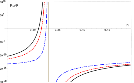
Figure 1: $\rho_{\rm rad}/\rho_{\rm tach}$ as a function of $n$ for the power law tachyon potential $V=\theta^{-4n}$ for $\kappa=$ 3 (full black line), 6 (dashed red), and 9 (dash-dotted blue). The vertical line indicates the critical power $n=1/3$.

From (64) we find

$$\chi_{\rm f}^{3-1/n}=\frac{\kappa^{2}}{2(3n+1)},$$ (106)

yielding

$$h_{\rm f}=\sqrt{\frac{2n(3n+1)}{3}}\left(\frac{2(3n+1)}{\kappa^{2}}\right)^{1/(3n-1)}.$$ (107)

Using this and (105) we obtain

$$\rho_{\rm rad}=\frac{C_{n}(3n-1)^{2}n^{6}k^{4}}{24\pi(8.31)^{2}}(3n+1)^{\frac{7n+1}{3n-1}}2^{\frac{5n+3}{3n-1}}\kappa^{-\frac{8}{3n-1}},$$ (108)

where the coefficient

$$C_{n}=\frac{2^{12}\cdot 8.31^{2}}{3^{7}\pi(3n+1)^{13}}\left(\frac{3n+1}{2}\right)^{2n/(3n-1)}\left(150n^{3}+85n^{2}-3\right)^{2}$$ (109)

is a smooth function of $n$ for $n\geq 0$ assuming the maximal value of 1.018447 at $n=0.316770$.

For the tachyon energy density we obtain the lower bound

$$\rho_{\rm tach}\gtrsim\frac{10^{10}nk^{4}}{24\pi(8.31)^{2}}(3n+1)^{\frac{7n+1}{3n-1}}2^{\frac{7n+1}{3n-1}}\kappa^{-\frac{2n+6}{3n-1}},$$ (110)

yielding an estimate of the ratio

$$\frac{\rho_{\rm rad}}{\rho_{\rm tach}}\lesssim C_{n}n^{5}(3n-1)^{2}\cdot 10^{-10}\left(\frac{\kappa}{2}\right)^{(2n-2)/(3n-1)}.$$ (111)

Note that for $\kappa>2$, the reheating is enhanced for $n>1$ and $n<1/3$. In the limit $n\rightarrow\infty$ the power of $\kappa$ approaches 2/3 yielding the enhancement as in the exponential case. In the limit $n\rightarrow 1/3$ from below the righthand side of (111) diverges, hence the ratio $\rho_{\rm rad}/\rho_{\rm tach}$can be arbitrary large for $n$ sufficiently close to $1/3$. Thus, in order to obtain a significant enhancement we need $\kappa>2$ and $n$ below and close to 1/3. The inequality $\kappa>2$ implies

$$h_{\rm f}\gtrless\sqrt{\frac{2n(3n+1)}{3}}\left(\frac{(3n+1)}{2}\right)^{1/(3n-1)}\quad{\rm for}\quad n\lessgtr 1/3.$$ (112)

The right hand side of this inequality is a monotonously increasing function of $n$ taking the values of 0.921321, 1, 1.099148, at $n$ equal to 1/4, 0.286106, and 1/3, respectively. Roughly, this means that a significant enhancement requires $h_{\rm f}>1$ to wit $H_{\rm f}>k$. In figure 1 we plot the ratio $\rho_{\rm rad}/\rho_{\rm tach}$ as a function of $n$ for various values of $\kappa>2$.

5 Conclusions

We have investigated the reheating in a braneworld inflationary scenario based on coupling of the tachyon with the abelian gauge field and the cosmological creation of massless particles. Assuming the tachyon potential of the inverse power $V\propto\theta^{-4n}$ we have shown that the cosmological creation of massless particles vanishes for critical power $n=1/2$ in the standard cosmology and $n=1/3$ in BWC. Next, we have shown that the reheating due to cosmological particle creation is insignificant in the standard cosmology whereas in BWC the reheating depends strongly on the power and can be significantly enhanced for powers $n$ approaching a critical point $n=1/3$ from below.

Unfortunately this scenario alone cannot solve the reheating problem of the tachyon inflation. It has been shown [8, 22] that the energy density of the tachyon with an inverse power potential yields asymptotically either dust or quasi de sitter universe, with the cosmological scale dependence as $\rho_{\rm tach}\propto a^{-3}$ or $1/\log a$, respectively. Since the radiation density behaves as $\rho_{\rm rad}\propto a^{-4}$, sooner or later $\rho_{\rm tach}$ will inevitably dominate the radiation.

It would be of considerable interest to investigate the effects of cosmological creation in the warm inflation models [37]. In warm inflation, radiation due to dissipative effects is produced in parallel with the inflationary expansion and inflation ends when the universe heats up to become radiation dominated. This scenario has been successfully applied to tachyon inflation models [38, 39] and, in principle, should also work for tachyon inflation in BWC presented here.

References

- [1] M. Fairbairn and M. H. G. Tytgat, Phys. Lett. B 546, 1 (2002) [hep-th/0204070]; A. Feinstein, Phys. Rev. D 66, 063511 (2002) [hep-th/0204140]; A. V. Frolov, L. Kofman and A. A. Starobinsky, Phys. Lett. B 545, 8 (2002) [hep-th/0204187]; G. Shiu and I. Wasserman, Phys. Lett. B 541, 6 (2002) [hep-th/0205003]; M. Sami, P. Chingangbam and T. Qureshi, Phys. Rev. D 66, 043530 (2002) [hep-th/0205179]; G. Shiu, S. H. H. Tye and I. Wasserman, Phys. Rev. D 67, 083517 (2003) [hep-th/0207119]; P. Chingangbam, S. Panda and A. Deshamukhya, JHEP 0502, 052 (2005) [hep-th/0411210]; S. del Campo, R. Herrera and A. Toloza, Phys. Rev. D 79, 083507 (2009) [arXiv:0904.1032]; S. Li and A. R. Liddle, JCAP 1403, 044 (2014) [arXiv:1311.4664].
- [2] L. Kofman and A. D. Linde, JHEP 0207, 004 (2002) [hep-th/0205121].
- [3] J. M. Cline, H. Firouzjahi and P. Martineau, JHEP 0211, 041 (2002) [hep-th/0207156].
- [4] D. A. Steer and F. Vernizzi, Phys. Rev. D 70, 043527 (2004) [hep-th/0310139].
- [5] A. Sen, JHEP 9910, 008 (1999) [hep-th/9909062].
- [6] S. E. Shandera and S.-H. H. Tye, JCAP 0605, 007 (2006) [hep-th/0601099].
- [7] N. Ohta, Int. J. Mod. Phys. A 20, 1 (2005) [hep-th/0411230].
- [8] L. R. W. Abramo and F. Finelli, Phys. Lett. B 575, 165 (2003) [astro-ph/0307208].
- [9] A. D. Dolgov and D. P. Kirilova, Sov. J. Nucl. Phys. 51 (1990) 172 [Yad. Fiz. 51 (1990) 273].
- [10] J. H. Traschen and R. H. Brandenberger, Phys. Rev. D 42 (1990) 2491. doi:10.1103/PhysRevD.42.2491
- [11] L. Kofman, A. D. Linde and A. A. Starobinsky, Phys. Rev. Lett. 73, 3195 (1994) [hep-th/9405187].
- [12] Y. Shtanov, J. H. Traschen and R. H. Brandenberger, Phys. Rev. D 51 (1995) 5438 doi:10.1103/PhysRevD.51.5438 [hep-ph/9407247].
- [13] L. Kofman, A. D. Linde and A. A. Starobinsky, Phys. Rev. D 56, 3258 (1997) [hep-ph/9704452].
- [14] B. A. Bassett, S. Tsujikawa and D. Wands, Rev. Mod. Phys. 78, 537 (2006) [astro-ph/0507632].
- [15] L. Randall and R. Sundrum, Phys. Rev. Lett. 83, 4690 (1999)
- [16] S. Kobayashi, K. Koyama and J. Soda, Phys. Rev. D 65, 064014 (2002) [arXiv:hep-th/0107025].
- [17] G. German, A. Herrera-Aguilar, D. Malagon-Morejon, R. R. Mora-Luna and R. da Rocha, JCAP 1302, 035 (2013) [arXiv:1210.0721 [hep-th]].
- [18] M. Bordemann and J. Hoppe, Phys. Lett. B 325, 359 (1994); N. Ogawa, Phys. Rev. D 62, 085023 (2000).
- [19] R. Jackiw, (2002) Lectures on Fluid Mechanics (Springer Verlag, Berlin, 2002).
- [20] M. Kalb and P. Ramond, Phys. Rev. D 9 2273 (1974).
- [21] C.V. Johnson, D-Branes (Cambridge University Press, Cambridge, 2003).
- [22] N. Bilić, S. Domazet and G. S. Djordjevic, Class. Quant. Grav. 34, 165006 (2017) [arXiv:1704.01072 [gr-qc]].
- [23] G. W. Gibbons and C. A. R. Herdeiro, Phys. Rev. D 63 064006 (2001).
- [24] N. Bilić, G. B. Tupper and R. D. Viollier, J. Phys. A 40, 6877 (2007) [gr-qc/0610104].
- [25] N. Bilić and D. Tolić, Phys. Rev. D 88, 105002 (2013) [arXiv:1309.2833 [gr-qc]].
- [26] N. Bilić and D. Tolić, Phys. Rev. D 91, 104025 (2015) [arXiv:1412.3977 [gr-qc]].
- [27] L. Parker, J. Phys. A 45, 374023 (2012) [arXiv:1205.5616 [astro-ph.CO]].
- [28] L. Parker, Ph.D. thesis, Harvard University, 1966; Phys. Rev. Lett. 21, 562 (1968); Phys. Rev. 183, 1057 (1969).
- [29] Th. De Donder, Théorie Invariantive Du Calcul des Variations (Gaultier- Villars & Cia., Paris, 1930); H. Weyl, Annals of Mathematics 36, 607 (1935).
- [30] J. Struckmeier, A. Redelbach, Int. J. Mod. Phys. E 17 435-491 (2008), [arXiv:0811.0508 [math-ph]]; C. Cremaschini and M. Tessarotto, Appl. Phys. Res. 8, no. 2, 60 (2016) [arXiv:1609.04422 [gr-qc]].
- [31] N. Bilić and G. B. Tupper, Central Eur. J. Phys. 12, 147 (2014) [arXiv:1309.6588 [hep-th]].
- [32] P. Binetruy, C. Deffayet and D. Langlois, Nucl. Phys. B 565, 269 (2000) [hep-th/9905012]; E. E. Flanagan, S. H. Henry Tye and I. Wasserman, Phys. Rev. D 62, 044039 (2000) [hep-ph/9910498].
- [33] N. Bilić, D. Dimitrijevic, G. Djordjevic and M. Milosevic, Int. J. Mod. Phys. A 32, no. 05, 1750039 (2017) [arXiv:1607.04524 [gr-qc]].
- [34] D. J. Schwarz, C. A. Terrero-Escalante and A. A. Garcia, Phys. Lett. B 517, 243 (2001) [astro-ph/0106020].
- [35] D. Baumann and L. McAllister, “Inflation and String Theory”,Cambridge University Press, 2015, arXiv:1404.2601 [hep-th].
- [36] L.H. Ford, Phys. Rev. D 35, 2955 (1987)
- [37] A. Berera, Phys. Rev. Lett. 75, 3218 (1995), [astro-ph/9509049]; A. Berera, Phys. Rev. D 54, 2519 (1996), [hep-th/9601134].
- [38] R. Herrera, S. del Campo and C. Campuzano, JCAP 0610, 009 (2006), [astro-ph/0610339]; S. del Campo, R. Herrera and J. Saavedra, Eur. Phys. J. C 59, 913 (2009) [arXiv:0812.1081].
- [39] M. R. Setare and V. Kamali, JHEP 1303, 066 (2013) [arXiv:1302.0493]; A. Bhattacharjee and A. Deshamukhya, Mod. Phys. Lett. A 28, 1350036 (2013), [arXiv:1302.1272]; X. M. Zhang and J. Y. Zhu, JCAP 1402, 005 (2014), [arXiv:1311.5327]; M. R. Setare and V. Kamali, Phys. Lett. B 736, 86 (2014) [arXiv:1407.2604]. A. Cid, Phys. Lett. B 743, 127 (2015) [arXiv:1503.00714]; M. Motaharfar and H. R. Sepangi, Eur. Phys. J. C 76, no. 11, 646 (2016) [arXiv:1604.00453 [gr-qc]]; V. Kamali, S. Basilakos and A. Mehrabi, Eur. Phys. J. C 76, no. 10, 525 (2016) [arXiv:1604.05434 [gr-qc]].