Antiresonant quantum transport in ac driven molecular nanojunctions

Abstract

We calculate the electric charge current flowing through a vibrating molecular nanojunction, which is driven by an ac voltage, in its regime of nonlinear oscillations. Without loss of generality, we model the junction by a vibrating molecule which is doubly clamped to two metallic leads which are biased by time-periodic ac voltages. Dressed-electron tunneling between the leads and the molecule drives the mechanical degree of freedom out of equilibrium. In the deep quantum regime, where only a few vibrational quanta are excited, the formation of coherent vibrational resonances affects the dressed-electron tunneling. In turn, back action modifies the electronic ac current passing through the junction. The concert of nonlinear vibrations and ac driving induces quantum transport currents which are antiresonant to the applied ac voltage. Quantum back action on the flowing nonequilibriun current allows us to obtain rather sharp spectroscopic information on the population of the mechanical vibrational states.

I Introduction

Fascinating progress has been achieved in downsizing artifically made condensed-matter devices. The study of micromechanical systems has evolved towards nanoelectromechanical systems (NEMS) that are at the core of molecular scale electronicsFerdin2017 . Thereby, the fundamental physical limits set by the laws of quantum mechanics are rapidly approached. The ultimate potential for nanoelectromechanical devices is governed by the ability to detect motional response to various external stimuli giving a variety of physical phenomena including electronic correlations Choi2017 as well as magnetism and other spin-related effects Kiran2017 ; Gaudenzi2017 ; Gaudenzi2017 . Molecular vibrations Kocic2017 and junction mechanics Hybertsen2017 are also under consideration in view of their thermal properties Cui2017 ; Tan2017 .

Several experimental realizations of nanoscale systems exist which display mechanical vibrations, such as, for instance, transversely vibrating nanobeams or lithographically patterned doubly clamped suspended beams LaHaye04 . Also suspended doubly clamped carbon nanotubes exhibit a rich mechanical vibrational spectrum Safavi2012 . Applications as electrometersCleland1996 ; Cleland1998 for detecting ultrasmall forces and displacements LaHaye04 ; Beil00 have been reported. Also NEMS are used for radio-frequency signal processing Nguyen99 and chemical sensoring Mohanty08 ; Mohanty06 . Other NEMS application include signal amplification in ultrasmall devices Mohanty07a ; Mohanty07b and spin readout techniques Mohanty04 . Fundamental physical phenomena emerge in NEMS due to the interplay of electronic and mechanical degrees of freedom, often immersed into a nonequilibrium environment Shekhter06 ; Regal08 ; Hansen2017 .

Due to their size, NEMS are of interest when studying the crossover from the classical to the quantum regime, where quantum fluctuations in transverse vibrations may drastically influence the dynamics Carr01 ; Carr01a ; Werner04 . The possibility of observing macroscopic quantum coherence is viable, since the quantized mechanical motion (phonons) involves a macroscopic number of particles forming the nanobeam. Yet, coherence is significantly disturbed by the interaction with the environment resulting in damping and decoherence Imboden14 . Experiments have reported measurements of the nonlinear response of a radiofrequency mechanical resonator which allows to obtain precise values of relevant mechanical parameters of the resonator Aldridge05 , as well as the cooling of the resonator motion by parametric coupling to a driven microwave-frequency superconducting resonator Rocheleau2010 .

Most techniques used to detect and actuate NEMS in view of the quantum behavior of their motion address linear response properties of transverse vibrations around their eigenfrequencies. In order to measure the response to various external stimuli, experiments require an increased resolution of the position measurement to the sub-thermal state Beil00 ; LaHaye04 ; Poggio2007 ; Safavi2012 ; MacQuarrie2017 . As the response of a damped linear quantum oscillator has a Lorentzian shape, similar to a damped linear classical oscillator Weiss1993 ; Chan2011 , a unique identification of the quantum behavior of a nanoresonator in the regime of linear vibrations is sometimes hard to perform.

Interestingly, pronounced quantum features arise when driven damped nonlinear quantum resonators are considered. These are typically induced by the interplay of the nonlinearity and the external periodic driving peanoPRB ; peanoCP ; peanoNJP ; peanoJCM1 ; peanoJCM2 ; Vicente1 ; Vicente2 . In the case of a driven dissipative quantum oscillator with a quartic nonlinearity, the oscillation amplitude in the steady state shows distinct quantum antiresonances for particular values of the driving frequencies peanoPRB ; peanoCP ; peanoNJP . At those values, multiphoton transitions occur which are accompanied by a phase slip of the response relative to the excitation, such that an antiresonant line shape of the response and a driving induced dynamical bistability arise. Similar response characteristics is generated in a quantum mechanical two-level system which is coupled to a harmonic oscillator in the presence of driving (either of the two-level system or the oscillator) peanoJCM1 ; peanoJCM2 . This driven dissipative Jaynes-Cummings model is also intrinsically nonlinear, leading to a comparable response in terms of quantum antiresonances. Since these antiresonances are associated to multiphoton transitions, they are in general very sharp. Hence, it has been proposed to use them for the state detection of quantum bits Vicente1 . In fact, the sharpness of the antiresonances also leads to interesting quantum noise properties of the multiphoton transitions Vicente2 . Yet, the detection of the sharp antiresonances remains difficult experimentally. This motivates the study of these effects in quantum transport setups, as suggested in the present work.

Further reduction in size from NEMS to molecular electronics has been pursued during recent years. From the experimental point of view, transport setups have the advantage that the current-voltage characteristics is accessible. Thus, it is an interesting question to search for nonlinear features in the mechanical motion of vibrating molecules. Important vibrational effects in the quantum transport in molecules concern phonon-assisted transport or non-linear vibrations Nitzan01 ; Nitzan ; molel ; Nitzan07 ; May04 , for a comprehensive review of vibrational effects in molecular transport, see Ref. Nitzan07, . Cizek, Thoss, and Domcke Thoss04 treat the inelastic regime by an electron-molecule scattering theory. In Ref. Flensberg03, , one vibrational mode has been investigated under the assumption of a strong electron-phonon coupling, which gives rise to rather strong tunneling broadening of the vibrational sidebands. A subsequent work Braig03 included additional damping of the vibrational mode. Vibrational effects in molecular transistors in the regime of sequential electron tunneling have also been investigated in Ref. Weiss2015, . Recently, implicit driving of the mechanical degrees of freedom induced by the electronic current has been revealed Jin2015 . The electrons which tunnel through a voltage-biased tunnel junction drive a transmission line resonator out of equilibrium. Further, an external periodic bias voltage can modify the distribution of molecular vibrations and the fluctuations of the molecular displacement Ueda2017 . Moreover, the emission noise of a conductor can drive the state of a single-mode cavity coupled to a voltage-biased quantum point contact Mendes2016 . When the molecular bridge has a permanent magnetic moment and a sizable magneto-mechanical coupling, the concept of nanocooling has been developed recently Brueggemann2014 ; Brueggemann2016 , in which a spin-polarized electronic current is used to locally control the magnetic moment which may reduce the thermal population of the mechanical vibrational mode and thus cool it.

Current-induced non-equilibrium vibrations in single molecule devices have been investigated in Refs. Koch05, ; Ueda2016, ; Ueda2017, , again in the incoherent regime. The impact of external light fields on electronic transport has been analysed in detail in Ref. Kohler05, . Moreover, charge transport through a vibrating molecule has been studied in terms of Keldysh Green’s function perturbatively in the electron-phonon coupling Ueda2017 ; Egger07 . Also nonequilibrium phonon dynamics in nanobeams and the related phonon-assisted losses have been investigated in Ref. Haertle2015, .

Antiresonances in quantum transport set-ups do not only occur when mechanical vibrations are present. In general, they can arise whenever nonlinear elements in a transport geometry occur. For instance, antiresonances in the conductance of a ferromagnetic lead with a side-coupled quantum dot can occur on the level of a treatment in terms of the Landauer formula due to interference of a resonant and a nonresonant transport path through the system FengPhysica2005 . Likewise, when several quantum dots are arranged in different geometries (in series, in parallel, etc.), the intrinsic transport features also become nonlinear and resonances and antiresonances arise the current-voltage spectrum JAP2009 . Also, Fano-type antiresonances occur in the linear conductance as a function of the gate voltage in a multi-dot set-up when the tunneling coupling between the dot system and the leads is asymetric JAP2012 . Yet, the occurrence of antiresonances in a mechanically vibrating nanojunction has not been discussed so far in the literature.

In this work, we are interested in the interplay of nonlinear molecular vibrations and an external ac driving, in particular in the deep quantum regime. We shall consider a molecular junction where its mechanical degree of freedom is described by a monostable nonlinear oscillator with a Kerr nonlinearity, while its electronic degree of freedom is modelled as a single electronic level (quantum dot approximation). This carries the electrons tunneling through the system to two noninteracting electronic leads. In addition, a periodically modulated bias voltage in the leads is considered in order to drive the system out of equilibrium, [cf. Fig. 1]. We consider the regime of weak electromechanical interaction in which independent single-electron tunneling processes between the leads and the junction modulate the junction’s mechanical motion and may induce few-phonon transitions. We in particular identify the signatures of the nonlinear vibrations in the charge current flowing through the nanobeam. Moreover, we find Fano-shaped resonances in the current, which are, in fact, antiresonances and which can be traced back to nonlinear resonances in the mechanical quantum dynamics.

In Sec. II, we introduce the Hamiltonian model. The rotating wave approximation is invoked and a time-dependent effective Hamiltonian is derived in Sec. II.2. Within a quantum master equation approach, discussed in Sec. III, we evaluate the current in the rotating as well as in the laboratory frame. We present our results in Sec. IV. Finally we conclude our findings in Sec. V.

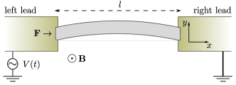
Figure 1: Sketch of a suspended nanobeam of length $l$ clamped between two metallic leads. We consider a constant external force ${\bf F}$, applied in the longitudinal direction of the nanobeam (along the $x$-axis). Additionally, in order to control the electromechanical coupling, we assume a transversal external magnetic field ${\bf B}=B_{0}\hat{e}_{z}$. The system is driven out of equilibrium by a time-dependent bias voltage $V(t)$.

II Model of an ac-driven nonlinear nanojunction

The setup of the molecular nanojunction depicted in Fig. 1 includes a suspended nanobeam of length $l$, doubly clamped to normal conducting leads in the presence of a time-dependent electrostatic potential $V(t)$. An external magnetic field ${\bf B}$ is applied perpendicular to the longitudinal axis of nanobeam to couple the mechanical motion to the electronic degrees of freedom. Electrons can tunnel from the leads into a single electronic level of the nanobeam, which is assumed to form a quantum dot. The Hamiltonian is

$$H(t)=H_{e}+H_{em}+H_{m}+H_{t}+H_{leads}(t)\,.$$ (1)

Here, $H_{e}$ is the Hamiltonian for the electrons passing through the nanobeam, $H_{em}$ describes the coupling between the electronic and the mechanical degree of freedom, and $H_{m}$ contains the mechanical degree of freedom with nonlinear bending deflections induced by an external force ${\bf F}=F\hat{e}_{x}$ in longitudinal direction. The tunneling of electrons from (to) the leads is accounted for by $H_{t}$ and $H_{leads}(t)$ covers the dynamics of noninteracting electrons in the leads.

For the electron dynamics, we consider only one longitudinal energy state with energy $E$, associated with the motion of electrons along the nanobeam, yielding

$$H_{e}=E\,\hat{d}^{\dagger}\hat{d}\ ,$$ (2)

where $d^{\dagger}$ ($d$) creates (destroys) an electron on the nanobeam.

For the mechanical dynamics, we want to consider the effect of a nonlinear vibrational mode of the nanojunction. The nonlinearity stems from the double clamping to the mechanical oscillator. To illustrate this in principle, we may consider a doubly clamped mechanical nanobeam. A nonlinear term can be easily obtained Werner04 by a constant longitudinal external force ${\bf F}=F\hat{e}_{x}$ with $F$ being close to the Euler buckling instability $F_{c}={\cal EI}(\pi/l)^{2}$, with $\cal E$ being Young’s modulus of elasticity and $\cal I$ the area momentum of inertia. Close to this unstable point, the fundamental mode vanishes and higher modes and nonlinear effects become relevant. Then, the bending deflections can be modeled by a single nonlinear vibrational mode Werner04 (we set $\hslash=1$)

$$H_{m}=\omega_{0}\,\hat{n}+\nu\,(\hat{b}^{\dagger}+\hat{b})^{4}/12\ ,$$ (3)

where

$$\omega_{0} = 4\left(\frac{\pi}{l}\right)^{2}\left[\frac{\cal EI}{3\rho_{b}}\cdot\frac{F_{c}-F}{F_{c}}\right]^{1/2}\ ,$$ (4)

$$\nu = \frac{4F_{c}-F}{{\cal EI}\rho_{b}\,l}\cdot\frac{F_{c}}{F_{c}-F}\ ,$$ (5)

are the fundamental frequency of the bending mode and the Kerr nonlinearity, respectively. Above, we have denoted by $\hat{n}=\hat{b}^{\dagger}\,{b}$ the phonon number operator. Intrinsically, the bending deflections affect the electronic dynamics through a very weak electromechanical coupling that depends on an even power of the nanobeam’s deflection amplitude Weick2010 ; Rastelli2012 . This coupling is enhanced by the application of an external magnetic field. Hence, the electromechanical coupling is tunable, where the electromagnetic force exerting on the electrons depends on the bending of the nanobeam. For the sake of simplicity, we consider the magnetic field applied in the $z$-direction perpendicular to the nanobeam’s longitudinal axis [cf. Fig. 1]. It has been shown in Ref. Rastelli2012, that the resulting electromechanical coupling might be written as

$$H_{em}=i\omega_{0}\phi(\hat{b}^{\dagger}-\hat{b})\hat{d}^{\dagger}\hat{d}\,,$$ (6)

where the dimensionless coupling constant is given by

$$\phi=\frac{\pi B_{0}Y_{0}l}{\Phi_{0}}\int_{0}^{l}ds\,\frac{u_{0}(s)}{l}\,.$$ (7)

Here, the magnitude of the external magnetic field is denoted by $B_{0}$, $Y_{0}$ is the amplitude of the zero point motion of the oscillator, the magnetic flux $\Phi_{0}=2\pi/e$ and $u_{0}(s)$ is the profile of the fundamental bending mode normalizedRastelli2012 according to $\int_{0}^{l}dsu_{0}^{2}(s)/l=1$.

Instead of considering a nanobeam, a linear molecule, e.g., a carbon nanotube, can be used in a doubly clamped configuration and excited to its nonlinear regime. For specific molecules, the mechanical modes can be determined numerically, but eventually lead to a model in the form discussed above.

The tunneling coupling between the system’s electronic state and the conducting leads is provided by the tunneling Hamiltonian

$$H_{t}=\sum_{p\,=\,l,\,r}H_{p}^{+}+H_{p}^{-}\ ,$$ (8)

$${\rm with}\quad H^{-}_{p}=\sum_{k}T_{{p},k}\,\hat{d}\ \hat{c}^{\dagger}_{p,k},\ \quad H^{+}_{p}=(H_{p}^{-})^{\dagger}.$$

Here, $\hat{c}^{\dagger}_{p,k},(\hat{c}_{p,k})$ creates (annihilates) an electron in the lead $p=l,r$. The coupling strengths are characterized by $T_{p,k}$, which induce a finite lifetime $\tau$ for electrons in the nanobeam. Hence, a broadening of width $\Gamma=1/\tau$ is generated for the electronic level of the nanobeam. In the standard wide-band limit approximation, one can neglect the energy dependence of the tunneling constants, i.e., $T_{p,k}\rightarrow T_{p}$, and assumes a constant level broadening $\Gamma\propto\sum_{p}|T_{p}|^{2}$. Later on, we study the weak coupling limit where $\Gamma\ll\Delta E,\omega_{0}$, with $\Delta E$ being the spacing of the quantized energies in the beam.

The leads are described by noninteracting electrons in the presence of an ac voltage $V(t)=V_{0}\cos(\omega_{\rm ex}t)$. Here, $V_{0}$ is the magnitude of the ac-driving voltage and $\omega_{\rm ex}$ the corresponding driving frequency. The resulting electrostatic potential difference renders the single-particle electronic energies in each lead time-dependent, according to $E_{p,k}(t)=E_{p,k}+eV_{p}(t)$, with $V_{p=r,l}(t)=\pm V(t)/2$ and $E_{p,k}$ being the electronic energies in each lead $p$. This results in the Hamiltonian

$$H_{leads}(t)=\sum_{p,k}E_{p,k}(t)\hat{c}^{\dagger}_{p,k}\hat{c}_{p,k}.$$ (9)

II.1 Time-dependent transformation of the Hamiltonian

It is convenient to transform the time dependence in Eq. (9) together with the coupling term Eq. (6) to the tunneling term Eq. (8) by a unitary transformation Shekhter06 ; Rastelli2012 ; Segal17

$${\cal U}(t)=\exp\left[\sum_{k,p}\varphi_{p}(t)\hat{c}^{\dagger}_{p,k}\hat{c}_{p,k}+i\phi(\hat{b}^{\dagger}+\hat{b})\hat{d}^{\dagger}\hat{d}\right]\,.$$ (10)

Here, $\varphi_{p}(t)={\rm e}\int_{0}^{t}ds\,V_{p}(s)=(v_{p}/\omega_{\rm ex})\sin(\omega_{\rm ex}t)$ is the phase accumulated by the bias voltage with $v_{p}=\pm eV_{0}$. The result of the transformed tunneling term Eq. (8) reads

$$H_{t}^{\prime}(t)=\sum_{p}\exp[-ie\varphi_{p}(t)+i\phi(\hat{b}^{\dagger}+\hat{b})]\,H^{-}_{p}+{\rm h.c.}\ ,$$ (11)

and, for Eq. (9) we find

$$H_{leads}^{\prime}=\sum_{p,k}E_{p,k}\hat{c}^{\dagger}_{p,k}\hat{c}_{p,k}\,.$$ (12)

Note that after the transformation, all time-dependent interactions, which influence the resonator externally, are shifted to the time-dependent tunneling term Eq. (11). The Hamiltonian can thus be rewritten as

$$H(t)=H_{e}+H_{m}+H_{t}^{\prime}(t)+H_{leads}^{\prime}.$$ (13)

It is convenient to rewrite Eq. (11) as an expansion in orthogonal polynomials

$$H_{t}^{\prime}(t) = \sum_{p}\sum_{nmm^{\prime}}\left[J_{n}(v_{p}/\omega_{\rm ex})e^{in\omega_{\rm ex}t}\right]\left[e^{-\phi^{2}/2}\frac{(i\phi)^{m+m^{\prime}}}{m!m^{\prime}!}({b}^{\dagger})^{m}{b}^{m^{\prime}}\right]H_{p}^{-}+{\rm h.c.}\,,$$

where we have used the Jacobi-Anger identity $\exp[i(v_{p}/\omega_{\rm ex})\sin(\omega_{\rm ex}t)]=\sum_{n}J_{n}(v_{p}/\omega_{\rm ex})e^{in\omega_{\rm ex}t}$ for the accumulated phase $\varphi_{p}(t)$ with $J_{n}(z)$ being the $n$th ordinary Bessel function of the first kind. In addition, we have used the identity $e^{i\phi(\hat{b}^{\dagger}+\hat{b})}=e^{-\phi^{2}/2}e^{i\phi\hat{b}^{\dagger}}e^{i\phi{b}}$. With these expansions, we define a new tunneling operator

$$\hat{\cal T}_{p,n}(v_{p},\phi)=e^{-\phi^{2}/2}J_{n}(v_{p}/\omega_{\rm ex})e^{i\phi\hat{b}^{\dagger}}e^{i\phi\hat{b}}\,\hat{d}.$$ (15)

In order to illustrate the relevance of this term in the dynamics of the system, we project the above expression onto the basis $\{|k,q\rangle\}$, with $|k\rangle$ and $|q\rangle$ being the eigenstates of the bosonic and the fermionic number operators, respectively. This means $\hat{n}=\hat{b}^{\dagger}\hat{b}$ and and $\hat{n}|k\rangle=k|k\rangle$, and likewise, $\hat{n}_{e}=\hat{d}^{\dagger}\hat{d}$, and $\hat{n}_{e}|q\rangle=n_{e}|q\rangle$. Note that $n_{e}=0$ or $1$ for $|q\rangle=|-\rangle$(unoccupied) or $|+\rangle$(occupied), respectively. Thus, the non-vanishing matrix elements of the projected tunneling operator read

$$\langle k-|\hat{\cal T}_{p,n}(v_{p},\phi)|l+\rangle = J_{n}(v_{p}/\omega_{\rm ex})\left(\sqrt{\frac{h_{k,l}!}{h_{l,k}!}}\,e^{-\phi^{2}/2}\,(i\phi)^{|k-l|}\,L_{h_{k,l}}^{|k-l|}(\phi^{2})\right),$$

with $L_{n}^{\alpha}(z)$ denoting the generalized Laguerre polynomials of degree $n$, and

$$h_{k,l}=k+\left(l-k\right)\Theta(k-l).$$

The magnitude of the tunneling matrix elements in Eq. (II.1) are limited by the bounds of the Bessel functions $\left|J_{k}(v_{p}/\omega_{\rm ex})\right|\leq c/{v_{p}}^{1/3}$ with $c=0,7853...$ Abramowitz1965 , and

$$\left|\sqrt{\frac{h_{k,l}!}{h_{l,k}!}}\,e^{-\phi^{2}/2}\,(i\phi)^{|k-l|}\,L_{h_{k,l}}^{|k-l|}(\phi^{2})\right|\leq 1.$$

We emphasize that under these conditions, the weak coupling limit is valid also in the laboratory frame. Note that the structure of the projected tunneling term Eq. (II.1) is not in conflict with the assumption of the electronic lifetimes in the beam $\tau^{\prime}$ to be longer than the typical time scale $2\pi/\omega_{0}$. Hence, the level broadening $\Gamma_{n}\propto\sum_{p}|\hat{\cal T}_{n,p}|^{2}$ is still small and the weak coupling regime $\Gamma\ll\omega_{0}$ is realized for even moderate values of $V_{0}$ and $\phi$.

II.2 Rotating wave approximation

The quantum dynamics of the nanobeam for the choice of parameters $v_{l/r}\ll\omega_{0}$, $\phi\ll 1$, $\nu\ll\omega_{0}$, and small detuning $\delta\omega\ll\omega_{0}$, with

$$\delta\omega\equiv\omega_{0}-\omega_{\rm ex}\,,$$ (17)

is most conveniently described in the co-rotating frame of reference, for which we apply a further unitary transformation

$$R(t)=\exp[-i\,(\hat{n}+\hat{d}^{\dagger}\hat{d})\,\omega_{\rm ex}t]\,.$$ (18)

In this rotating frame, the typical time scale of the system dynamics is given by $\delta\omega^{-1}$, such that terms oscillating with frequencies $\pm n\omega_{\rm ex}$ for $n\geq 1$ are averaged out and may be neglected in the transformed Hamiltonian $H^{\prime}(t)=R(t)H(t)R^{\dagger}(t)-iR(t)\dot{R}^{\dagger}(t)$. For instance, applying the transformation of Eq. (18) to the quartic term in Eq. (3), we obtain $R(t)(\hat{b}+\hat{b}^{\dagger})^{4}R^{\dagger}(t)=6\hat{n}(\hat{n}+1)+O(\hat{b}^{2}\exp[-2i\omega_{\rm ex}t])+O(\hat{b}^{\dagger 2}\exp[2i\omega_{\rm ex}t])+3$, and in an appreciable amount of time, the terms $\propto\exp[\pm in\omega_{\rm ex}t]$ for $n=2$ and $4$ will quickly average to zero, such that the relevant term in the quartic potential is $6\hat{n}(\hat{n}+1)+3$.

Within this rotating wave approximation (RWA), we find the Hamiltonian

$$H^{\prime}=H^{\prime}_{e}+H^{\prime}_{m}+H^{\prime}_{t}+H^{\prime}_{leads},$$ (19)

where

$$H^{\prime}_{e} = \delta\omega\,\hat{d}^{\dagger}\hat{d}$$ (20)

$$H^{\prime}_{m} = \delta\omega\,\hat{n}+\nu\,\hat{n}(\hat{n}+1)/2,$$ (21)

$$H^{\prime}_{t} = \sum_{p,k}\hat{\cal T}^{\prime}_{p}(v_{p},\phi)\,\hat{c}_{k,p}^{\dagger}+{\rm h.c.}$$ (22)

Here, the tunneling operator

$$\hat{\cal T}^{\prime}_{p}(v_{p},\phi)=T_{p}e^{-\phi^{2}/2}\sum_{nm}J_{n}(v_{p}/\omega_{\rm ex})\frac{(i\,\phi)^{2m+n-1}}{m!(n+m-1)!}\,(\hat{b}^{\dagger})^{m}\,\hat{b}^{n+m-1}\hat{d},$$ (23)

has the matrix elements $\langle k-|\hat{\cal T}^{\prime}_{p}(v_{p},\phi)|l+\rangle=\langle k-|\hat{\cal T}_{p,l-k+1}(v_{p},\phi)|l+\rangle$ (cf. Eq. (II.1)). In passing, we note that both unitary transformations given in Eqs. (10) and (18) commute with each other in the weak coupling regime in which the sequential tunneling approximation made below holds. Clearly, $R(t)$ as well as $\mathcal{U}(t)$ induce higher-order coupling terms within the transformed tunneling Hamiltonian which are beyond the sequential tunneling approximation used here. Moreover, for the tunneling term, the criteria of fast oscillating terms used in the rotating wave approximation is not sufficient to state that the contribution given in Eq. (23) is dominant over the neglected counter-propagating terms, and so the validity of the approximation needs to be verified. In the rotating frame, the tunneling term can be written as

$$\hat{\cal T}_{p}^{\,r}(v_{p},\phi,t)=\sum_{n}\hat{t}_{n,p}(v_{p},\phi)\,e^{in\omega_{\rm ex}t}\,,$$ (24)

where $\langle k-|\hat{t}_{n,p}(v_{p},\phi)|l+\rangle=\langle k-|\hat{\cal T}_{p,l-k+1+n}(v_{p},\phi)|l+\rangle$. Thus for a small bias voltage, characterized by $v_{p}/\omega_{\rm ex}\ll 1$, the ratio between the matrix elements of the counter-propagating terms (for $n>0$ in Eq. (24)) and the co-propagating ones ($n=0$) reads as

$$\frac{\langle k-|\hat{t}_{n,p}(v_{p},\phi)|l+\rangle}{\langle k-|\hat{t}_{0,p}(v_{p},\phi)|l+\rangle}\sim\frac{\Gamma(l-k+1)}{\Gamma(l-k+1+n)}\left(\frac{v_{p}}{2\omega_{\rm ex}}\right)^{n}\ll 1\,.$$ (25)

Consequently, the contribution of the counter-propagating terms is negligible in the solution of the system dynamics, and the rotating-wave approximation, in which $\hat{\cal T}^{\prime}_{p}(v_{p},\phi)\equiv\hat{t}_{0,p}(v_{p},\phi)$, is justified.

III Quantum master equation

The dynamics of the system described by the Hamiltonian (19) is fully characterized by the statistical operator $W(t)$, whose time evolution is governed by the von-Neumann equation

$$\frac{d}{dt}W(t)=-i[H(t),W(t)]\,.$$ (26)

After tracing out the degrees of freedom of the leads, we obtain the reduced system, represented by the density operator $\rho\equiv{\rm Tr}_{\rm leads}[W]$. In addition, in the weak coupling regime considered throughout this work, $\Gamma\ll\omega_{0}$, it is possible to express the evolution of the reduced density operator in terms of a diagrammatic expansion in the tunneling terms $H_{p}^{\pm}$ Weiss2015 ; Konig1996a . We use the standard Born-Markov approximation (for a recent discussion, see Ref. Dubi2017, ) and, furthermore, exploit a high-frequency approximation which is valid when the ac-voltage drive is much faster than the mechanical oscillations. Then, the master equation for the reduced density operator reads

$$\frac{d}{dt}\rho(t)=-i[H_{0},\rho(t)]+\Sigma\cdot\rho(t)\ ,$$ (27)

in which the first term on the right hand size represents the nanobeam coherent dynamics, with

$$H_{0}=\delta\omega\,d^{\dagger}d+\delta\omega\,\hat{n}+\nu\,\hat{n}\,(\hat{n}+1)/2\ ,$$ (28)

and the second term represents dissipation and decoherence induced by tunneling events between leads and the beam. This part is covered by the self-energy $\Sigma=\Sigma_{r}+\Sigma_{l}$, therein $\Sigma_{p}$ is the contribution from lead $p$. In leading order in $\Gamma$, the self energy $\Sigma_{p}$ is composed by eight terms corresponding to different tunneling events $\Sigma_{p}=\sum_{n=1}^{8}\Sigma_{p}^{(n)}$ (see Appendix A for details).

III.1 Electron current in the rotating frame

The electronic current operator $\hat{I}_{p}$ from the lead $p$ to the nanobeam is given by the charge in the number of electrons in lead $p$ over time. We use the number operator of lead $p$ as $\hat{n}_{p}=\sum_{k}\hat{c}^{\dagger}_{k}\hat{c}_{k}$ and find

$$\hat{I}^{\prime}_{p}(t) = -e\dot{\hat{n}}_{p}=-e[H^{\prime}_{t}(t),\hat{n}_{p}]$$ (29)

$$= \sum_{k}\left(\hat{\cal T}^{\prime}_{p}(v_{p},\phi)\hat{c}^{\dagger}_{p,k}(t)\,-{\rm h.c.}\right)\ .$$

The net current passing through the nanobeam is

$$\hat{I}^{\prime}_{\rm rwa}(t)\equiv\hat{I}^{\prime}_{l}(t)-\hat{I}^{\prime}_{r}(t)\,.$$ (30)

We are left with calculating the expectation value $I^{\prime}_{p}(t)=\langle\hat{I}_{p}\rangle_{t}\equiv{\rm Tr}[\rho(t)\hat{I}_{p}]$, which is determined from the self-energies and for which we find

$$I^{\prime}_{p}(t)=-ie\left\langle\Sigma_{p}^{(5)}(t)+\Sigma_{p}^{(8)}(t)-\Sigma_{p}^{(6)}(t)-\Sigma_{p}^{(7)}(t)\right\rangle.$$ (31)

III.2 Electron current in the laboratory frame

In the previous section, the electron current has been expressed in terms of the self-energies $\Sigma_{p}^{(5),(8)}(t)$ and $\Sigma_{p}^{(6),(7)}(t)$ in the rotating frame. For a better interpretation, we consider in this section the current in the laboratory frame.

Since the Hamiltonian is periodic in time, we can expand the diagrams in terms of Fourier vectors $|f_{m}\rangle$, $m\in\mathbb{Z}$, such that $\langle t|m\rangle=e^{-im\omega_{\rm ex}t}$. With this, the expectation value of the current becomes

$$I(t)=\sum_{m=-\infty}^{\infty}I_{m}\,e^{-im\omega_{\rm ex}t}$$ (32)

with the Fourier coefficients $I_{m}=I_{l,m}-I_{r,m}$, where

$$I_{p,m} =-ie\left\langle\Sigma^{(5)}_{p,m}(\omega_{\rm ex})+\Sigma^{(8)}_{p,m}(\omega_{\rm ex})\right.$$

$$\left.-\Sigma^{(6)}_{p,m}(\omega_{\rm ex})-\Sigma^{(7)}_{p,m}(\omega_{\rm ex})\right\rangle\,.$$ (33)

Here, $\Sigma^{(i)}_{p,m}(\omega_{\rm ex})$ denotes the $m$-th Fourier component of $\Sigma^{(i)}_{p}(t)$, i.e., $\Sigma^{(i)}_{p}(t)=\sum_{m=-\infty}^{\infty}\Sigma^{(i)}_{p,m}(\omega_{\rm ex})e^{-im\omega_{\rm ex}t}$.

The stationary value for $m=0$ and the higher harmonics ($m\neq 0$) of the current are associated to different single-electron tunneling processes. The modulation in the bias voltage splits the energy levels of the leads into sidebands separated by $\omega_{\rm ex}$.Tien1963 Thus, a lead state $|k\rangle_{p}$, on lead $p$ and with energy $E_{k,p}$, is split into a set of states $\{|k_{n}\rangle_{p}\}$ with energies $E_{nk,p}=E_{k,p}+n\omega_{\rm ex}$, where $n$ is an integer and determines the order of the sideband.

In the undriven case, the transfer of an electron from the left to right lead occurs via an energy level $E$ in the corresponding transport window characterized by $\mu_{r}<E<\mu_{l}$, where $\mu_{p}$ is the corresponding electrochemical potential of the lead $p$. On the other hand, for the driven case, the condition for sequential transport is not straightforward, since the occupied states on the right lead can be above the Fermi level, i.e., there exists an $n$ such that $E_{nk,r}>\mu_{r}$ although $E_{k,r}<\mu_{r}$ and a reduction of the electronic current is generated. Another interesting mechanism occurs when an occupied sideband level on the left lead can reach the level energy of the central system. This occurs when $E_{nk,l}=E$ for $E_{k,l}\neq E$, and the electron can tunnel to the right lead to a sideband level of energy $E_{kn^{\prime},r}=E$ for $E_{k,r}>\mu_{r}$. There, an electron can transport $|n-n^{\prime}|$ quanta of energy absorbed from the external modulation. The current $I_{p}$ is given by the sum over all the possible tunneling events from sidebands on the left lead to sidebands on the right lead. If we denote by $P_{nn^{\prime}}$ the probability of a tunneling event from the sideband $|k_{n}\rangle_{l}$ to the sideband $|k_{n^{\prime}}\rangle_{r}$, the current can be rewritten in the form

$$I_{p}=e\sum_{nn^{\prime}}P_{nn^{\prime}}=\sum_{j=-\infty}^{\infty}\left(\sum_{n-n^{\prime}=j}eP_{n,n-j}\right).$$ (34)

This sum can be reordered according to the number of quanta of energy exchange between the leads. Then, $\sum_{n-n^{\prime}=m}eP_{nn-m}$ resembles the aforementioned component $I_{p,m}$ and the stationary current corresponds to $\sum_{n-n^{\prime}=0}eP_{nn}$.

We are interested in the current for one-phonon processes characterized by

$$I_{\rm rwa}(t)=I_{-1}\exp[i\omega_{\rm ex}t]+I_{1}\exp[-i\omega_{\rm ex}t]\,,$$ (35)

whose oscillation amplitude in leading order of $v_{p}$ and $\phi$ corresponds to the current in the rotating frame, i.e.,

$$I_{\rm rwa}\equiv{\rm max}_{t}\,I_{\rm rwa}(t)=2|I_{1}|\,.$$ (36)

IV Quantum antiresonances

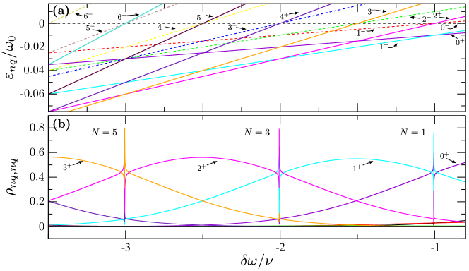
Figure 2: (a) Quasienergy spectrum for $\phi=0$ and (b) state populations (diagonal elements of the reduced density operator) for $\phi=5\times 10^{-2}$ as a function of the detuning frequency. The labels $0^{-},1^{-},2^{-},...,6^{-}$ (dashed lines) mark the states for the electronically unoccupied nanobeam corresponding to the quasienergies $\varepsilon_{n-}$ in (a) and the populations $\rho_{n-n-}$ in (b) for $n=0,1,...,6$. Likewise, the labels $0^{+},1^{+},2^{+},...,6^{+}$ (continuous lines) mark the electronically occupied nanobeam corresponding to the quasienergies $\varepsilon_{n+}$ in (a) and the populations $\rho_{n+;n+}$ in (b) for $n=0,1,2,...,6$. The parameters used in these simulations are $\Gamma=10^{-3}\omega_{0}$, $\nu=10^{-2}\omega_{0}$, $E=\omega_{0}$, $V_{l}=-V_{r}=10^{-2}\omega_{0}$, $\mu_{l}-\mu_{r}=10\,\omega_{0}$, and $k_{\rm B}T=5\times 10^{-3}\omega_{0}$.

In general, switching off adiabatically the electromechanical coupling $\phi\rightarrow 0$, mechanical and electronic subsystem decouple and the energy levels of the nanaobeam increase by multiples of the mechanical nonlinear strength $\nu$ according to Eq. (28) as

$$\varepsilon_{n+1,q}-\varepsilon_{n,q^{\prime}}=\delta\omega(1+n_{q}-n_{q^{\prime}})+\nu(n+1)\,.$$ (37)

We label the eigenstates by $|n,q\rangle$, where $n=0,1,2,\dots$ denotes the quantum number of the vibrational state and $q=+,-$ refers to the quantum number of the electronic state, respectively. Since we use a spinless model, we have two possible electronic eigenstates of the dot, either the occupied or the unoccupied state for the occupation number operator $n_{q}=d^{\dagger}d$. Suppose that $N$ quanta of energy have been exchanged between the two subsystems, then several non-equidistant resonances will appear in the spectrum. They are quantified by the quasienergy $\varepsilon_{N-n,q}=\varepsilon_{n,q^{\prime}}$, i.e., the detuning should be chosen as

$$\delta\omega=-\frac{\nu}{2}\,\,\frac{N(N+1)}{N+n_{q}-n_{q^{\prime}}}\,.$$ (38)

Note that for the nontrivial case $N>0$, the detuning is always negative $\delta\omega<0$. In Fig. 2(a), the quasi-energy spectrum, for $\phi=0$, as a function of the ratio $\delta\omega/\nu$ is shown. Exact crossings occur whenever the condition of Eq. (38) is met, indicating a degeneracy between two quasienergies. Note that for the linear Holstein model Weiss2015 , when $\nu=0$, all degeneracies are absent. For $\phi\neq 0$, the degeneracy is lifted and the states $|N-n,q\rangle$ and $|n,q^{\prime}\rangle$ are mixed by the interaction terms, see Eq. (22). They generate the anticrossings of the quasienergy levels in the spectum. Around a given (anti-)resonance, the states $|N-n,q\rangle$ and $|n,q^{\prime}\rangle$ are mixed strongest (see Fig. 2(b)). The mixing results in the corresponding dressed states $|\varphi_{n}\rangle$ and $|\varphi_{N-n}\rangle$, which are superpositions of the two localized states $|N-n,q\rangle$ and $|n,q^{\prime}\rangle$. As an analogy, one might think of a static double-well potential, where for a finite overlap between the two degenerate states (referred to as tunneling), the left and right energy eigenstates are mixed and the spectrum forms an anticrossing when the bias between the two wells is changed. Here, we would identify the left and right localized states with the pairwise resonant states $|N-n,q\rangle$ and $|n,q^{\prime}\rangle$. Naturally, the role of the ’tunneling’ is played by the electromechanical coupling $\phi$, which induces a coupling between the two states and thus generates transitions.

In the laboratory frame, the electrons couple to the mechanical motion via the operator $\hat{b}^{\dagger}-\hat{b}$, see Eq. (6). This means that the mechanical degree of freedom receives or releases energy, once the electronic state is occupied. Therefore, the most populated states are formed by the pair $|N-n,+\rangle$ and $|n,+\rangle$. This behavior is in analogy to the Duffing oscillator peanoPRB ; peanoCP ; peanoNJP , where at resonance the population is concentrated on those states, i.e., $\rho_{N-n,+}=\rho_{N,+}=1/2$.

On the other hand, the expansion used here, in leading order of $\Gamma$, considers transitions between nearest neighbor states. The transition dynamics between states of the vibrating nanojunction affects the sequential tunneling current when $N$ is an odd integer. In the picture of a bistable quasienergy surface peanoNJP , this amounts to a single phonon inter-well transition. The nearest-neighbor condition on $|\varphi_{(N-n)+}\rangle$ and $|\varphi_{n+}\rangle$ requires that $(N-n)-n=1$, such that $N$ is an odd number. Thus, in the case of the $N$-th resonance with $N$ being odd, the relevant states are $|N^{*}+1,+\rangle$ and $|N^{*},+\rangle$ with $N^{*}=(N-1)/2$.

Below, we aim at obtaining an approximate and simple expression for the line shape of the antiresonance in the current. For this, we need the approximate solution of the quantum master equation in the vicinity of an avoided crossing of a pair of quasienergy states. In leading order of the voltage, i.e., of the ratio $v_{p}/\omega_{\rm ex}$, and of $\phi$, we keep the terms for $(n,m)=(0,1)$ and $(n,m)=(1,0)$ in the tunneling operator in Eq. (23), which yields to a simplified expression in the form

$$\hat{\cal T}^{\prime}_{p}(v_{p},\phi)\approx\frac{v_{p}}{2\omega_{\rm ex}}\mathbb{I}_{\rm mech}\hat{d}+i\,\phi\,\hat{b}^{\dagger}\hat{d}\,.$$ (39)

We used $J_{1}(v_{p}/\omega_{\rm ex})\approx v_{p}/(2\omega_{\rm ex})$ and $J_{0}(v_{p}/\omega_{\rm ex})\approx 1$. Above, $\mathbb{I}_{\rm mech}=\sum_{n}|n\rangle\langle n|$ is the identity operator in the Hilbert subspace of the mechanical degrees of freedom with the basis $\{|n\rangle\}$. The above expression Eq. (39) yields the self-energies

$${}^{n+}_{n+}\left[\Sigma_{p}^{(5)}+\Sigma_{p}^{(8)}\right]_{m-}^{m-} \approx (n+1)\,\phi^{2}\,\Gamma_{p}\,f^{-}_{p}[-\nu(n+1)]\,\delta_{m,n+1}$$

$${}^{m-}_{m-}\left[\Sigma_{p}^{(6)}+\Sigma_{p}^{(7)}\right]_{n+}^{n+} \approx (n+1)\,\phi^{2}\,\Gamma_{p}f^{+}_{p}[-\nu(n+1)]\,\delta_{m,n+1}$$

where $f_{p}^{\pm}(\epsilon)=\{\exp[\pm(\epsilon-\mu_{p})]+1\}^{-1}$ is the probability distribution of an occupied ($+$) or an unoccupied ($-$) electronic state in the lead $p$. The self-energies Eqs. (IV) and (IV) represent transition rates between different mechanical states which are relevant for the current calculation. It follows that the coupling with the leads only induces transitions between nearby mechanical states within this single-phonon approximation.

The external bias voltage modulation induces a transition from $|N^{*},+\rangle$ to $|N^{*}+1,+\rangle$, while electron tunneling generates transitions between nearby mechanical states. As a consequence, the ratio $\rho_{n+;n+}/\rho_{n+1,+;n+1,+}$ is given by the ratio of the corresponding transition rates as

$$\frac{\rho_{n+;n+}}{\rho_{n+1,+;n+1,+}}=\frac{\quad\quad\quad{}^{n+}_{n+}\left[\Sigma^{(5)}_{p}+\Sigma^{(8)}_{p}\right]_{(n+1)-}^{(n+1)-}}{{}^{(n+1)+}_{(n+1)+}\left[\Sigma^{(5)}_{p}+\Sigma^{(8)}_{p}\right]_{n-}^{n-}}\approx\frac{n+1}{n+2}\,.$$ (42)

Taking into account that $\rho_{N^{*}+;N^{*}+}=\rho_{N^{*}+1,+;N^{*}+1,+}$, the states $|\varphi_{N^{*}+}\rangle$ and $|\varphi_{N^{*}+1,+}\rangle$ are the states with the largest occupation probability.

To summarize, the electrons on the leads exchange energy with the external modulation, thereby getting dressed. Then, a dressed electron tunnels to the central system sending the mechanical motion out of equilibrium due to the electromechanical coupling. Depending on the external frequency, the mechanical motion can exchange energy with the electrons affecting the amplitude of the electronic current. This provides feedback to the current. This process is similar to controling the thermal occupation of the vibrational mode of magnetic Brueggemann2014 ; Brueggemann2016 and non-magneticWeiss2015 molecular junctions by an external spin current. There, the magnetic moment and the vibrational mode interact via a magnetomechanical coupling, yielding to an exchange of energy in the way that the vibrational energy can be transferred to the magnetic degree of freedom, which overall implies vibrational cooling of the nanojunction.

In panel (b) of Fig. 2, the steady-state populations of the system are depicted as a function of the external frequency. The most populated states correspond to $\rho_{N^{*}+1,+;N^{*}+1,+}$ and $\rho_{N^{*}+;N^{*}+}$. Out of resonance, all the states are equally populated and $\rho_{nq;nq}=1/(2\bar{N})$, with $\bar{N}$ being the number of states covered within the bias window $\mu_{l}-\mu_{r}$. For the $N$th resonance when $N$ is even, the most populated state is $\rho_{N/2,+;N/2,+}$ and $\rho_{N/2+1,+;N/2+1,+}=\rho_{N/2-1,+;N/2-1,+}$ due to the single excitation process induced by the current. Those states are dominant. Therefore, $\rho_{N/2,+;N/2,+}+\rho_{N/2+1,+;N/2+1,+}+\rho_{N/2-1,+;N/2-1,+}\approx 1$ as it is shown in the panel (b) of Fig. 2.

IV.1 Signatures in the electronic current

From Eqs. (IV) and (IV), we obtain directly an analytic approximation for the electronic current in the rotating frame (cf. Eq. (31))

$$I^{\prime}_{p}(v_{p},\phi)\approx\phi^{2}\,\Gamma_{p}\,\sum_{n}(n+1)\left(f^{-}_{p}[-\nu(n+1)]\rho_{n+;n+}-f^{+}_{p}[-\nu(n+1)]\rho_{n-;n-}\right).$$ (43)

The first (second) term on the right hand side in Eq. (43) corresponds to the current of out-coming (incoming) electrons from (into) the central system, respectively. Around the $N$th resonance when $N$ is odd, the populations $\rho_{N^{*}+;N^{*}+}$ and $\rho_{N^{*}+1,+;N^{*}+1,+}$ are dominant and the current simplifies to

$$I^{\prime}_{p}(v_{p},\phi) \approx \phi^{2}\,\Gamma_{p}\,(N^{*}+1)f^{-}_{p}[-\nu(N^{*}+1)]$$

$$\quad\quad\times\left(\rho_{N^{*}+;N^{*}+}+\rho_{N^{*}+1,+;N^{*}+1,+}\right).$$

With this at hand, we can calculate the current amplitude $I_{\rm rwa}=2|I_{1}|$ of Eq. (36) in the laboratory frame.

Following a similar procedure used for the calculation of the current (IV.1), we write the tunneling operator $\hat{t}_{n,p}(v_{p},\phi)$ in leading order of $v_{p}$ and $\phi$ and calculate the relevant self-energies $\Sigma_{p}^{5,8}$ and $\Sigma_{p}^{6,7}$. Then, the current amplitude for the $n$-phonon process, for $n>1$, is given by $I_{n}=J_{n-1}^{2}(v_{p}/\omega_{\rm ex})I_{\rm rwa}$. Consequently, $I_{n}/I_{\rm rwa}<(v_{p}/\omega_{\rm ex})^{2n-2}\ll 1$, which shows that the contribution from the co-rotating terms are also dominant for the current. The amplitude $I_{\rm rwa}$ of the current flowing through the central system is shown in panel (b) of Fig. 3 as a function of the detuning of the external driving frequency (blue continuous line). The blue solid lines indicate the calculated full mean value Eq. (30) without further approximation. We find pronounced antiresonances at particular values of the detuning. The current describes an asymmetric line-shape resonance determined by the resonance condition established in Eq. (38) for $N$ odd. Inside panel (b), a zoom of the current behavior around the antiresonance is shown. In addition, we also show the current calculated using the approximation Eq. (IV.1) (orange dots). Both results agree well which underlines that the argumentation yielding us to the approximation is correct. The antiresonances are similar to those obtained for the dissipative quantum Duffing oscillator peanoPRB ; peanoCP ; peanoNJP and those of the driven dissipative Jaynes-Cummings model peanoJCM1 ; peanoJCM2 and they have a Fano-type form due to the fact that a discrete quantum level interacts with a continuum of electronic energy levels.

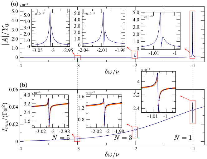
Figure 3: (a) Amplitude of the mechanical vibration, and, (b) the amplitude of the first harmonic of the ac current $I_{\rm rwa}=2|I_{1}|$, Eq. (36), as a function of the detuning frequency $\delta\omega$. The parameters used in these simulations are $\phi=5\times 10^{-2}$, $\Gamma=10^{-3}\omega_{0}$, $\nu=10^{-2}\omega_{0}$, $E=\omega_{0}$, $V_{l}=-V_{r}=10^{-2}\omega_{0}$, $\mu_{l}-\mu_{r}=10\,\omega_{0}$, $k_{B}T=5\times 10^{-3}\omega_{0}$.

In this regime, in which $v_{p}/\omega_{\rm ex}\ll\phi$, the time-averaged input-output power $P(\omega_{\rm ex})=\omega_{\rm ex}\langle d\hat{n}/dt\rangle$ is proportional to the electron current (IV.1), i.e.,

$$P(\omega_{\rm ex}) = -i\omega_{\rm ex}\langle\left[H^{\prime}_{t},\hat{n}\right]\rangle$$

$$\approx -i\omega_{\rm ex}\sum_{p}p\langle\Sigma_{p}^{(5)}+\Sigma_{p}^{(8)}-\Sigma_{p}^{(6)}+\Sigma_{p}^{(7)}\rangle.$$

This means in turn that measuring the electrical current gives insight into the population of the mechanical states and the flux of excitations put into the motion of the clamped beam.

IV.2 Antiresonant mechanical nonlinear response

According to Eq. (IV.1), the electronic current drives the mechanical degree of freedom out of equilibrium. An interesting consequence for the mechanical motion is the nonlinear response of the nonlinear nanobeam to the external ac driving of the bias voltage. We are thus interested in the nonlinear response of the mechanical motion characterized by the mean value $A$ of the position operator in the steady state, defined by

$$A=\frac{Y_{0}}{\sqrt{2}}\;{\rm Tr}[(\hat{b}+\hat{b}^{\dagger})\rho]\,.$$ (46)

Here, $Y_{0}$ is the amplitude of the zero point fluctuations in the nanobeam’s fundamental bending mode. Note that this mean value corresponds to the oscillation amplitude of the expectation value of the position operator in the laboratory reference frame. Therefore, we denote $A$ as the amplitude of the nonlinear response.

Around the $N$th resonance ($N$ odd), the quasi-energy difference between $|\varphi_{N^{*},+}\rangle$ and $|\varphi_{N^{*}+1,+}\rangle$ becomes smaller than $\Gamma$. We can consider $|\varphi_{N^{*},+}\rangle\approx(|N^{*},+\rangle+|N^{*}+1,+\rangle)/\sqrt{2}$ and $|\varphi_{N^{*}+1,+}\rangle\approx(|N^{*},+\rangle-|N^{*}+1,+\rangle)/\sqrt{2}$. With this, we find

$$A\approx\frac{Y_{0}}{\sqrt{2}}\sqrt{N^{*}+1}\left(\rho_{N^{*},+;N^{*},+}-\rho_{N^{*}+1,+;N^{*}+1,+}\right)\,.$$ (47)

The contribution from off-diagonal elements add up to zero due to $\rho_{N^{*},+;N^{*}+1,+}=\rho^{*}_{N^{*},+;N^{*}+1,+}$.

At resonance, each state of the corresponding pair has the same occupation probability, $\rho_{N^{*},+;N^{*},+}=\rho_{N^{*}+1,+;N^{*}+1,+}$, and the nonlinear response amplitude vanishes $A=0$. Away from resonance the pair-wise states are localized, $|\varphi_{N^{*},+}\rangle=|N^{*},+\rangle$ and $|\varphi_{N^{*}+1,+}\rangle=|N^{*}+1,+\rangle$, and their quasi-energy difference is larger than the tunneling constant $\Gamma$. Therefore, the off-diagonal elements of the density matrix are negligible, yielding $A=0$. In Fig. 3 (a), the amplitude of the nonlinear response is depicted as a function of the external frequency. Again, the amplitude exhibits quantum antiresonances around the $N$th resonance ($N$ odd). Since this antiresonance appears in the current spectrum, it should in principle be directly measurable.

V Conclusions

The interplay of a dissipative nonlinear quantum mechanical resonator with an external periodic driving is known to generate nontrivial response properties of the resonator in the form pronounced and rather sharp quantum antiresonances. The detection of those is non-trivial. In this work, we proposed to use a molecular nanojunction (or, a nanobeam) in its regime of nonlinear mechanical oscillations and clamped to conducting leads. This junction carries electronic current when an ac driving voltage is applied. An applied static magnetic field controls the electromechanical coupling of the flowing electron current and the mechanical oscillation. A static longitudinal compression force close to the Euler buckling instability may be used to tune the nonlinearity. Then, the mechanical oscillation amplitude can be described by an effective single particle quantum harmonic oscillator Hamiltonian with a weak Kerr nonlinearity. For the electronic part, we consider weak tunneling contact between the junction and the lead. The first longitudinal energy eigenstate is associated with the motion of the electrons along the nanobeam, such that a quantum dot is formed.

In the regime of weak electromechanical coupling, and considering a finite lifetime of the electrons in the nanojunction being longer than the typical time scale of intrinsic junction dynamics, the non-equilibrium dynamics is captured by a Born-Markov master equation. It has been formulated in a frame rotating with the ac driving frequency, in which the fast oscillating terms were average out. The effective model Hamiltonian of the molecule shows non-equidistant quasi-energy levels which define several resonant conditions which corresponds to multiquantum transitions in the nanobeam mechanical motion. In particular, the mechanical response reveals striking quantum antiresonances between pairs of quasienergy levels which for an anticrossing when, for instance, the driving frequency is varied. For modulation frequencies around the defined resonance conditions, the dynamics can be simplified by restricting to a two quasi-energy levels only. The solution may be used to determine the flowing electron current which is the observable being directly accessible in an experiment. The approximate picture is confirmed by solving the full master equation numerically and by calculating the net current passing through the nanobeam. Although we have presented results for a specific set of parameters in this work, especially the quantum master equation allows one to explore further regions of the parameter space. The observed effects will also survive in the regime of strong nonequilibrium quantum transport, where higher order phonon processes become important. We find that the feature of the quantum antiresonances in the mechanical response of the junction translates into antisymmetric line shape resonances in the electric charge current located at frequencies where the multiple transition in the mechanical motion takes place.

For very weak driving amplitudes of the ac voltage, we find a simple expression for the current which shows its direct dependence on the occupation probability of the mechanical antiresonant states. Along with the electronic current, a flux of energy into or out of the nanojunction can be determined, which drives the mechanical degree of freedom out of equilibrium. We find a similar structure of the nonlinear response of the nanojunction with that calculated for the quantum Duffing oscillator peanoPRB ; peanoCP ; peanoNJP . Moreover, the response is also similar to the driven dissipative Jaynes-Cummings model peanoJCM1 ; peanoJCM2 . Yet, the important difference in the present quantum transport set-up is that the quantum antiresonances are directly measurable in the current which renders the effect interesting for experimental observation.

Appendix A Quantum master equation approach

To obtain the dynamics of the central nanojunction only, it is convenient to trace out the electrodes’ degrees of freedom in the full density operator $W(t)$ of leads plus junction. In doing so in the interaction picture, the reduced density operator reads

$${\rho}^{I}(t) = {\rm Tr}_{l,\,r}\{{W}^{I}(t)\}$$

$$= {\rho}(t_{0})-i\int_{t_{0}}^{t}dt_{1}{\rm Tr}_{l,\,r}[{H}^{I}_{T}(t_{1}),{W}^{I}(t_{1})]\ ,$$

where ${\rm Tr}_{l,\,r}$ denotes the trace over the degrees of freedom of the right and left lead. Differentiating with respect to $t$, we obtain the quantum master equation for the reduced density operator,

$$\frac{d}{dt}{\rho}^{I}(t)=-\int_{t_{0}}^{t}dt_{1}\ {\rm Tr}_{l,\,r}\left\{[{H}^{I}_{T}(t),[{H}^{I}_{T}(t_{1}),{W}^{I}(t_{1})]]\right\}\,,$$ (49)

where, for simplicity, we have eliminated the term $-i{\rm Tr}_{l,\,r}\bigl{\{}[{H}^{I}_{T}(t),{W}^{I}(t_{0})]\bigr{\}}$ with the assumption ${\rm Tr}_{l,\,r}\bigl{\{}{H}^{I}_{T}(t){\rho}_{l}\otimes{\rho}_{r}\bigr{\}}=0$. This is equivalent to consider ${\rho}_{l}\otimes{\rho}_{r}$ as diagonal in energy basis, in other words, it is equivalent to the assumption that the leads are at their respective thermal equilibrium. ${W}^{I}$ factorizes at $t=t_{0}$, and at later times correlations between leads and the central system arise due to the tunneling term ${H}_{T}$. However, for a very weak coupling, at all times ${W}(t)$ should only show deviations of order ${H}_{T}$ from an uncorrelated state. Thus, in this regime of sequential electron tunneling, we can formulate a quantum master equation for $\rho$ in the form

$$\frac{d}{dt}{\rho}(t)=-i[{H}_{0},{\rho}(t)]+\int_{t_{0}}^{t}dt_{1}\,\Sigma(t,t_{1})\cdot{\rho}(t_{1})\ .$$ (50)

in the Schödinger picture. The first term on the right hand side in Eq. (50) governs the coherent dynamics, whereas the second term encloses all the effects of the fermionic bath covered by the kernel $\Sigma(t,t_{1})$. It includes self-energies, which are induced by the leads, in arbitrary orders in the tunneling. In a diagrammatic expansion of Eq. (50) Konig1996a , the selfenergy $\Sigma(t,t_{1})$ encloses only irreducible terms.

To calculate these irreducible diagrams, it is convenient to split the tunneling term ${H}_{t}$ into two parts, according to Eq. 8. In order to simplify the notation, we omit here the superscript for the interaction picture for the creation and annihilation operators. It is implicitly assumed unless stated otherwise. Then, the lowest order of the expansion of $\Sigma$ can be written as

$$\int_{t_{0}}^{t}dt_{1}\Sigma(t,t_{1}){\rho}(t)=\Sigma(t){\rho}(t)$$

$$= -{\cal T}_{K}\int_{K}ds\left(\underbrace{\left\langle{H}_{t}^{+}(t){H}_{t}^{-}(s)\,{\rho}(t)\right\rangle_{lr}}_{\Sigma^{(1)}(t,s)\cdot\rho(t)}+\underbrace{\left\langle{H}_{t}^{-}(t){H}_{t}^{+}(s){\rho}(t)\right\rangle_{lr}}_{\Sigma^{(2)}(t,s)\cdot\rho(t)}\right.$$

$$\quad\quad\quad\quad\ \,+\;\underbrace{\left\langle{\rho}(t){H}_{t}^{+}(s){H}_{t}^{-}(t)\right\rangle_{lr}}_{\Sigma^{(3)}(t)\cdot\rho(t)}+\underbrace{\left\langle{\rho}(t){H}_{t}^{-}(s){H}_{t}^{+}(t)\right\rangle_{lr}}_{\Sigma^{(4)}(t,s)\cdot\rho(t)}$$

$$\quad\quad\quad\quad\ \,-\;\underbrace{\left\langle{H}_{t}^{+}(t){\rho}(t){H}_{t}^{-}(s)\right\rangle_{lr}}_{\Sigma^{(5)}(t,s)\cdot\rho(t)}-\underbrace{\left\langle{H}_{t}^{-}(t){\rho}(t){H}_{t}^{+}(s)\right\rangle_{lr}}_{\Sigma^{(6)}(t,s)\cdot\rho(t)}$$

$$\quad\quad\quad\quad\ \,\left.-\,\underbrace{\left\langle{H}_{t}^{+}(s){\rho}(t){H}_{t}^{-}(t)\right\rangle_{lr}}_{\Sigma^{(7)}(t,s)\cdot\rho(t)}-\underbrace{\left\langle{H}_{t}^{-}(t_{1}){\rho}^{I}(t){H}_{t}^{+}(t)\right\rangle_{lr}}_{\Sigma^{(8)}(t,s)\cdot\rho(t)}\right)\ ,$$

where $\langle\cdots\rangle_{lr}={\rm Tr}_{l,\,r}\{(\cdots){\rho}_{l}\otimes{\rho}_{r}\}$. $K$ denotes the closed Keldysh contour which runs from $t_{0}$ to $t$ on the real axis and then back again from $t$ to $t_{0}$. Moreover, ${\cal T}_{K}$ denotes the corresponding time ordering operator on the Keldysh contour.

The formal solution of the quantum master equation Eq. (27) can be cast into the form

$${\rho}(t) = e^{{\cal L}\,t}{\rho}(0)=\sum_{k}{\rm Tr}\bigl{\{}{\rho}_{k}^{\dagger}{\rho}(0)\bigr{\}}\,e^{\Gamma_{k}t}\,{\rho}^{k}\ ,$$ (52)

where ${\cal L}{\rho}(t)\equiv-i[H_{0},\rho(t)]+\Sigma\rho(t)$, ${\rho}^{k}$ (${\rho}_{k}$) are the right (left) eigenoperators of ${\cal L}$ with eigenvalue $\Gamma_{k}$. The steady state is determined by the right eigenoperator ${\rho}^{k^{\prime}}\equiv{\rho}^{\infty}$ with the eigenvalue $\Gamma_{k^{\prime}}=0$. Therefore, the solution of the master equation is linked to the solution of a eigenvalue problem for a singular matrix.

Appendix B Charge current in the laboratory frame

We may use the expansion of the quantum master equation to derive an expression for the electric charge current. By definition, the current is given by the time derivative of the electron number $\hat{n}_{p}=\sum_{k}{c}_{k,p}^{\dagger}{c}_{k,p}$ on lead $p$, i.e., by

$$I_{p}(t) = -e\frac{d}{dt}\left\langle\hat{n}_{p}(t)\right\rangle=-ie\left\langle\bigl{[}{H}(t),\hat{n}_{p}(t)\bigr{]}\right\rangle$$ (53)

$$= -ie\left(\bigl{\langle}{H}^{+}_{t,p}(t)\rangle-\langle{H}^{-}_{t,p}(t)\bigr{\rangle}\right)\ .$$

In leading order of $\Gamma$, the current is determined by the components of the self energy, $\Sigma_{p}^{(5...8)}$,

$$I_{p}(t) = \sum_{m}I_{p,m}\,e^{i\,m\,\omega_{\rm ex}\,t}\,{\rm with}$$ (54)

$$I_{p,m} = -ie\left\langle\Sigma^{(5)}_{p,m}(\omega_{\rm ex})+\Sigma^{(8)}_{p,m}(\omega_{\rm ex})-\Sigma^{(6)}_{p,m}(\omega_{\rm ex})-\Sigma^{(7)}_{p,m}(\omega_{\rm ex})\right\rangle\,,$$

where, in order to calculate the current, we fix Weiss2015 one tunneling vertex in each of the diagrams at the measurement time $t$. Here, $\Sigma^{(i)}_{p,m}$ is the $m$th Fourier component of $\Sigma^{(i)}_{p}$. We symmetrize with respect to the leads, such that we compute the current $I(t)=I_{l}(t)-I_{r}(t)$. In the rotating frame of reference, after neglecting the fast oscillating terms, the calculated current correspond to the amplitude of the first mode in Eq. (54).

References

- (1) F. Evers and L. Venkataraman, J. Chem. Phys. 146, 092101 (2017).
- (2) D. Choi, P. Abufager, L. Limot, and N. Lorente, J. Chem. Phys. 146, 092309 (2017).
- (3) V. Kiran, S. R. Cohen, and R. Naaman, J. Chem. Phys. 146, 092302 (2017).
- (4) R. Gaudenzi, M. Misiorny, E. Burzurí, M. R. Wegewijs, and H. S. J. Van der Zant, J. Chem. Phys. 146, 092330 (2017).
- (5) N. Kocić, S. Decurtins, S. Liu, and J. Repp, J. Chem. Phys. 146, 092327 (2017).
- (6) M. S. Hybertsen, J. Chem. Phys. 146, 092323 (2017).
- (7) L. Cui, R. Miao, C. Jiang, E. Meyhofer, and P. Reddy, J. Chem. Phys. 146, 092201 (2017).
- (8) K. Y. Tan, M. Partanen, R. E. Lake, J. Govenius, S. Masuda, and M. Möttönen, Nat. Commun. 8, 15189 (2017).
- (9) M. D. LaHaye, O. Buu, B. Camarota, and K. Schwab, Science 304, 74 (2004).
- (10) A. H. Safavi-Naeini, J. Chan, J. T. Hill, T. P. M. Alegre, A. Krause, and O. Painter, Phys. Rev. Lett. 108, 033602 (2012).
- (11) A. N. Cleland and M. L. Roukes, Appl. Phys. Lett. 69, 2653 (1996).
- (12) A. N. Cleland and M. L. Roukes, Nature 392, 161 (1998).
- (13) F. W. Beil, L. Pescini, E. Höhberger, A. Kraus, A. Erbe, and R. H. Blick, Nanotechnology 14, 799 (2003).
- (14) C. T. C. Nguyen, A. C. Wong, and H. Ding, Dig. Tech. Pap.-IEEE Int. Solid-State Circuits Conf. 448, 78 (1999).
- (15) X. Wang, K. A. G. Y. Chen, S. Erramilli, and P. Mohanty, Appl. Phys. Lett. 92, 013903 (2008).
- (16) J. Dorignac, A. Kalinowski, S. Erramilli, and P. Mohanty, Phys. Rev. Lett. 96, 186105 (2006).
- (17) Y. Chen, X. Wang, M. K. Hong, S. Erramilli, P. Mohanty, and C. Rosenberg, Appl. Phys. Lett. 91, 243511 (2007).
- (18) R. L. Badzey and P Mohanty, Nature 437, 995 (2005).
- (19) P. Mohanty, G. Zolfagharkhani, S. Kettemann, and P. Fulde, Phys. Rev. B 70, 195301 (2004).
- (20) R. Shekhter, L. Gorelik, L. I. Glazman, and M. Jonson, Phys. Rev. Lett. 97, 156801 (2006).
- (21) C. A. Regal, J. D. Teufel, and K. W. Lehnert, Nature Phys. 4, 555 (2008).
- (22) T. Hansen, G. C. Solomon, and T. Hansen, J. Chem. Phys. 146, 092322 (2017).
- (23) S. M. Carr, W. E. Lawrence, and M. N. Wybourne, Phys. Rev. B 64, 220101 (2001).
- (24) S. M. Carr, W. E. Lawrence, and M. N. Wybourne, Physica B 316, 464 (2002).
- (25) P. Werner and W. Zwerger, Europhys. Lett. 65, 158 (2004).
- (26) M. Imboden and P. Mohanty, Phys. Rep. 534, 89 (2014).
- (27) J. S. Aldridge and A. N. Cleland, Phys. Rev. Lett. 94, 156403 (2005).
- (28) T. Rocheleau, T. Ndukum, C. MacKlin, J. Hertzberg, A. Clerk, and K. Schwab, Nature 463, 72 (2010).
- (29) M. Poggio, C. L. Degen, H. J. Mamin, and D. Rugar, Phys. Rev. Lett. 99, 017201 (2007).
- (30) E. R. MacQuarrie, M. Otten, S. K. Gray, and G. D. Fuchs, Nat. Commun. 8, 14358 (2017).
- (31) U. Weiss, Quantum Dissipative Systems 4th ed. (World Scientific, Singapore, 2012).
- (32) J. Chan, T. P. M. Alegre, A. H. Safavi-Naeini, J. T. Hill, A. Krause, S. Groblacher, M. Aspelmeyer, and O. Painter, Nature 478, 89 (2011).
- (33) V. Peano and M. Thorwart, Phys. Rev. B 70, 235401 (2004).
- (34) V. Peano and M. Thorwart, Chem. Phys. 322, 135 (2006).
- (35) V. Peano and M. Thorwart, New J. Phys. 8, 21 (2006).
- (36) V. Peano and M. Thorwart, Europhys. Lett. 89, 17008 (2010).
- (37) V. Peano and M. Thorwart, Phys. Rev. B 82, 155129 (2010).
- (38) V. Leyton, M. Thorwart, and V. Peano, Phys. Rev. B 84, 134501 (2011)
- (39) V. Leyton, V. Peano and M. Thorwart, New J. Phys. 14, 093024 (2012).
- (40) A. Nitzan, Annu. Rev. Phys. Chem. 52, 681 (2001).
- (41) A. Nitzan and M. Ratner, Science 300, 1384 (2003).
- (42) G. Cuniberti, G. Fagas, and K. Richter, Lecture Notes in Physics: Introducing Molecular Electronics (Springer, Berlin, 2005).
- (43) M. Galperin, M. Ratner, and A. Nitzan, J. Phys. Cond. Matt. 19, 103201 (2007).
- (44) V. May and O. Kühn, Charge and Energy Transfer Dynamics in Molecular Systems (Wiley-VCH, Weinheim, 2004).
- (45) M. Cizek, M. Thoss, and W. Domcke, Phys. Rev. B 70, 125406 (2004).
- (46) K. Flensberg, Phys. Rev. B 68, 205323 (2003).
- (47) S. Braig and K. Flensberg, Phys. Rev. B 68, 205324 (2003).
- (48) S. Weiss, J. Brüggemann, and M. Thorwart, Phys. Rev. B 92, 045431 (2015).
- (49) J. Jin, M. Marthaler, and G. Schön, Phys. Rev. B 91, 085421 (2015).
- (50) A. Ueda, Y. Utsumi, Y. Tokura, O. Entin-Wohlman, and A. Aharony, J. Chem. Phys. 146, 092313 (2017).
- (51) U. C. Mendes and C. Mora, Phys. Rev. B 93, 235450 (2016).
- (52) J. Brüggemann, S. Weiss, P. Nalbach, and M. Thorwart, Phys. Rev. Lett. 113, 076602 (2014).
- (53) J. Brüggemann, S. Weiss, P. Nalbach, and M. Thorwart, New J. Phys. 18, 023026 (2016).
- (54) J. Koch, M. Semmelhack, F. von Oppen, and A. Nitzan, Phys. Rev. B 73, 155306 (2006).
- (55) A. Ueda, Y. Utsumi, H. Imamura, and Y. Tokura, J. Phys. Soc. Jpn. 85, 043703 (2016).
- (56) S. Kohler, J. Lehmann, and P. Hänggi, Phys. Rep. 406, 379 (2005).
- (57) R. Egger and A. Gogolin, Phys. Rev. B 77, 113405 (2007).
- (58) R. Härtle and M. Kulkarni, Phys. Rev. B 91, 245429 (2015).
- (59) J.-F. Feng, X.-F. Jiang, J.-L. Zhong, and S.-S. Jiang, Physica B 365, 20 (2005).
- (60) Z. Z. Sun, R. Q. Zhang, W. Fan, and X. R. Wang, J. Appl. Phys. 105, 043706 (2009).
- (61) Y. Han, W.-J. Gong, H.-M. Wang, and A. Du, J. Appl. Phys. 112, 123701 (2012).
- (62) G. Weick, F. Pistolesi, E. Mariani, and F. von Oppen, Phys. Rev. B 81, 121409 (2010).
- (63) G. Rastelli, M. Houzet, L. Glazman, and F. Pistolesi, C. R. Phys. 13, 410 (2012).
- (64) B.K. Agarwalla and D. Segal, J. Chem. Phys. 147, 054104 (2017).
- (65) A. Zazunov and T. Martin, Phys. Rev. B 76, 033417 (2007).
- (66) L. Mühlbacher and E. Rabani, Phys. Rev. Lett. 100, 176403 (2008).
- (67) M. Abramowitz and I. A. Stegun, Handbook of Mathematical Functions (Dover, New York, 1965).
- (68) J. König, H. Schoeller, and G. Schön, Phys. Rev. Lett. 76, 1715 (1996).
- (69) A. Purkayashta and Y. Dubi, Phys. Rev. B 96, 085425 (2017).
- (70) P. K. Tien and J. R. Gordon, Phys. Rev. 129, 647 (1963).