Pair Correlation and Gap Distributions for Substitution Tilings and Generalized Ulam Sets in the Plane

Abstract

We study empirical statistical and gap distributions of several important tilings of the plane. In particular, we consider the slope distributions, the angle distributions, pair correlation, squared-distance pair correlation, angle gap distributions, and slope gap distributions for the Ammann Chair tiling, the recently discovered fifteenth pentagonal tiling, and a few pertinent tilings related to these famous examples. We also consider the spatial statistics of generalized Ulam sets in two dimensions. Additionally, we carefully prove a tight asymptotic formula for the time steps in which Ulam set points at certain prescribed geometric positions in their plots in the plane formally enter the recursively-defined sets.

The software we have developed to these generate numerical approximations to the distributions for the tilings we consider here is written in Python under the Sage environment and is released as open-source software which is available freely on our websites. In addition to the small subset of tilings and other point sets in the plane we study within the article, our program supports many other tiling variants and is easily extended for researchers to explore related tilings and iterative sets.

Keywords: substitution tiling; Ammann chair; Ulam set; directional distribution; gap distribution; pair correlation.
MSC Subject Class (2010): 52C20; 06A99; 11B05; 62H11; 52C23.
Last Revised:

1 Introduction

The study of the spatial statistics of various point sets in the plane, and in particular the use of these statistics as a comparison to random processes, is by now well-established (for example, see [6] and the references within). In this paper, we describe empirical statistics for various families of self-similar and pentagonal tilings, focusing in particular on two well-known (families of) tilings: special chair tilings, such as the Ammann chair, and the numbered Pentagonal tilings in Section 2.1 and Section 3, respectively. Additionally we consider generalized forms of Ulam sets in two dimensions, their spatial statistics, and formalize other properties related to these sets in Section 4. We hope that our work and the software we provide inspires more theoretical work on the study of limiting distributions for these point sets, and in particular proofs of existence and formulas for limiting gap distributions and pair correlation functions for angles, slopes, and distances.

1.1 A unified perspective on two-dimensional substitution tilings and Ulam sets

We begin by unifying perspectives on substitution tilings and two-dimensional Ulam sets, and their directional distribution statistics. In both situations we have a nested sequence of recursively-generated, or recursively-defined finite sets $A_{n}$, where nested means

$$A_{0}\subset A_{1}\subset\cdots\subset A_{n-1}\subset A_{n}.$$

We are interested in the limiting distribution of directions and the pair correlation plots in the sets $A_{n}$ as $n\rightarrow\infty$. The next two subsections define the specific classes of substitution tilings and two-dimensional Ulam set variants we consider within this article. In Section 1.2 below we define the specific forms of the directions and statistical plots which we compare in the next few sections.

1.1.1 Substitution tilings

We start with a polygon $P$ (with a vertex at the origin $0$) which as a decomposition into pieces $P_{1},\ldots,P_{k}$, each of which is affinely similar to the original polygon $P$, that is, there are affine maps $g_{i}$ so that $g_{i}(P)=P_{i}$ and

$$P=\bigcup_{i=1}^{k}P_{i}.$$

A map $g:\mathbb{R}^{2}\rightarrow\mathbb{R}^{2}$ is affine if

$$g(x)=hx+v,$$

where $h\in GL(2,\mathbb{R})$ and $v\in\mathbb{R}^{2}$. $A_{0}$ is the set of vertices of $P$, $A_{1}$ the set of vertices of $P_{1},\ldots P_{k}$. Now we can decompose

$$P_{i}=\bigcup_{j=1}^{k}g_{i}(P_{j}),$$

the sets of vertices of $g_{i}(P_{j}),i,j=1,\ldots,k$ forms $A_{2}$, and so on, at each stage decomposing each piece into smaller pieces. For example, if we take the square $[0,1]^{2}$ and its decomposition into quarters, we get finer and finer square grids, equivalently we could look at larger and larger subsets of the integer lattice. In this case, we know the distribution of the slope gaps of this complete “tiling” as Hall’s distribution.

1.1.2 Ulam sets

In this case, we start with $A_{0}$ given by a pair of vectors,

$$A_{0}=\{v_{0},v_{1}\},A_{1}=\{v_{0},v_{1},v_{0}+v_{1}\},$$

and to build $A_{n+1}$ from the set $A_{n}$ we add the shortest of the vectors by their Euclidean norms which can be written uniquely as the sum of two vectors in $A_{n}$. Note that this set will be in the wedge defined by $v_{0}$ and $v_{1}$. We let $A_{\infty}=\bigcup A_{n}$, and refer to this as the Ulam set associated to $v_{0},v_{1}$. In our special cases where we have only two initial vectors, we have by Kravitz-Steinerberger [13, Theorem 1] that these Ulam sets correspond to the following subset of the lattice points $\{mv_{0}+nv_{1}:m,n\in\mathbb{\mathbb{missing}}Z\cup\{0\}\}$ in the wedge: boundary points $v_{0}+nv_{1}$ and $nv_{0}+v_{1}$ for natural numbers $n\geq 0$ and inner points $mv_{0}+nv_{1}$ for $m,n\geq 3$ both odd positive integers (see Section 4.1).

These points are filled in gradually at different finite time steps: for $a,b\in\mathbb{Z}\cup\{0\}$ with $av_{0}+bv_{1}\in A_{\infty}$, let $K(a,b)$ denote the time of its appearance,

$$K(a,b)=\min\{n:av_{0}+bv_{1}\in A_{n}\}.$$

Consider the $n^{th}$ line segment

$$L_{n}=\{xv_{0}+yv_{1}:x,y\geq 0,x+y=n+1\}$$

consisting of points in the Ulam set $A_{\infty}$ on the segment between $nv_{0}+v_{1}$ and $v_{0}+nv_{1}$. In §4 we prove a refinement of [13, Theorem 1] in the context of our so-termed “timing distributions” which we define precisely in Section 4. In particular, we state and prove a more exact form of the next result which succinctly summarizes the statement of our key theorem proved in the sections below.

Theorem (Timing Distributions).

There are positive constants $C_{1},C_{2}$ such that for any $av_{0}+bv_{1}\in A_{\infty}\cap L_{n},$ we have that

$$C_{1}\cdot n^{2}\leq K(a,b)\leq C_{2}\cdot n^{2}.$$

To our knowledge the considerations of such timing distributions in the context of generalized Ulam sets are new and have not been considered elsewhere or in the references. The generalizations of the one-dimensional Ulam sequence to sequences of vectors in the plane is a fairly recent construction made by Kravitz and Steinerberger in 2017. Even fully classifying the plot structure, or inclusion properties of the lattice spanned by the initial vectors for $k\geq 3$ specified initial conditions remains an open problem. Thus there is much left to explore about the properties and graphs of these generalized Ulam sets in the plane, and our new results on the timing distributions of these sets is only a start to many other properties which we can approach by geometric arguments concerning these sets.

1.2 Definitions and statistical plots considered within the article

1.2.1 Directions

Given such a sequence of subsets of $\mathbb{R}^{2}$, we consider various statistics associated to the directions of points in $A_{n}$. For both Ulam and substitution, note that the set of possible angles (and slopes) is determined by the original set (either the polygon or the initial two vectors). So the set of directions (either slopes or angles) is contained in some interval $[a,b]$ (where for slopes we could have $a=-\infty$ or $b=\infty$, though often in examples we can use symmetry to reduce our set, for example, with the square substitution/integer grid, we can look at things of slope between $0$ and $1$).

1.2.2 Gap distributions and spatial statistics

For $x\in\mathbb{R}^{2}$, let $x=(x^{(1)},x^{(2)})$, and consider the slope and angle

$$s(x)=\frac{x^{(2)}}{x^{(1)}},\theta(x)=\arctan s(x).$$

Write

$$A_{n}=\{x_{1},\ldots x_{N}\}$$

where the resulting

$$s_{k}=s(x_{k}),\theta_{k}=\theta(x_{k})$$

are in increasing order. Of course $N=N_{n}$ depends on $n$. We are interested in (among other things) the limiting histogram distributions of the next sets and the following underlying questions about these distributions:

Equidistribution of slopes.

For $[c,d]\subset[a,b]$, does

$$\lim_{n\rightarrow\infty}\frac{\#\{1\leq k\leq N_{n}:s_{k}\in[c,d]\}}{N_{n}}=\frac{d-c}{b-a}\text{?}$$

Gap distributions.

Let $g_{i}=N_{n}(s_{i+1}-s_{i})$ (slope gaps) or $g_{i}=N_{n}(\theta_{i+1}-\theta_{i})$ (angle gaps). For $[c,d]\subset[0,\infty]$, does

$$\lim_{n\rightarrow\infty}\frac{\#\{1\leq k\leq N_{n}:g_{k}\in[c,d]\}}{N_{n}}$$

exist?

Pair correlation.

For $[c,d]\subset[0,\infty]$, does

$$\lim_{n\rightarrow\infty}\frac{\#\{1\leq j<k\leq N_{n}:N_{n}(x_{k}-x_{j})\in[c,d]\}}{N_{n}}$$

exist?

1.2.3 Some notes on obtaining limiting distributions

Gap distributions and pair correlation functions have been widely studied for various families of subsets of the plane, often arising from connections with low-dimensional dynamical systems and number theory. These include lattices, affine lattices, sets of saddle connections on translation surfaces (often arising from billiards in polygons), and more recently, cut-and-project quasicrystals, see, for example [1, 2, 3, 4, 9, 14, 7, 8, 15, 19, 20]. The methods of proof in these results vary, but a common thread in several is using dynamics and equidistribution of unipotent flows on an appropriate moduli space which parameterizes deformations of our point sets (see [1] for a general theorem regarding this strategy). In particular, this strategy is particularly effective when the original set has a large linear symmetry group.

The equidistribution of a sequence of finite lists $F(k)$ (here, the slopes or angles of our point sets $A_{k}$) can be viewed as a first-order test for randomness. In general, one considers the normalized gap sets

$$G(k):=\left\{N_{k}\left(F_{k}^{(i+1)}-F_{k}^{(i)}\right):0\leq i<N(k)\right\},$$

and given $0\leq a<b\leq\infty$, we consider the behavior of the proportion of gaps between $a$ and $b$, given by

$$\lim_{k\rightarrow\infty}\frac{\left|G(k)\cap(a,b)\right|}{N_{k}}.$$

If the sequence $F(k)$ is truly random, that is, given by

$$F(k)=\{X_{(0)}\leq X_{(1)}\leq\ldots\leq X_{(k)}\},$$

where the $\{X_{(i)}\}$ are the order statistics generated by independent, identically distributed (i.i.d.) uniform $[0,1)$ random variables $\{X_{n}\}_{n=0}^{\infty}$, the gap distribution has converges to a Poisson process of intensity $1$. Precisely, for any $t>0$,

$$\lim_{k\rightarrow\infty}\frac{\left|G(k)\cap(t,\infty)\right|}{N_{k}}=e^{-t}$$ (1)

In many of our examples, the empirical limiting gap distribution appears to be not Poissonian, thus giving some indication of the underlying ‘non-random’ structure of the sets.

1.3 New results and conjectures

1.3.1 Conjectures and new observations

Our experimental project provides the results of numerical computations performed on the Sage Math Cloud servers of the empirical distributions for the pair correlation, tiling point angles, tiling point slopes, and the corresponding gap distributions of the angles and slopes for more than $40$ well-known tilings of the plane [27, 26].

We predict that the individual angle and slope distributions equidistribute for sufficiently large $N$ (or equivalently points within some large radius $R<\infty$). We also pose several conjectures on the smoothness of the limiting distributions of the gap and pair correlation distributions of the chair and pentagon tilings we consider in Section 2 and in Section 3. We expect that due to the inwards recursive nature (deflation of subtiles rather than the scaling of inflation) we use to generate successive plots of the chair tiling examples that the pair correlation plots should be center-heavy with a monotone decrease towards either extreme at the tails of the distribution. That the limiting distributions for the gap and pair correlation plots appear to converge to smooth, piecewise continuous curves for large $N$ hints at more of the underlying structure of these important and interesting tiling variants. Given the interest of the chair tilings with respect to the group actions of $\mathbb{Z}^{2}$ and $\mathbb{R}^{2}$ on these tiling spaces (see, for example, [16, 17]), we also suggest the computations of the exact empirical distributions corresponding to these tilings as the subject of another computational research article.

In Section 2.1.3, we also connect the similarities between the gap distributions for the AmmannChair tiling, the saddle connections on the golden L studied in [3], and the TubingenTriangle tiling to the symmetry groups for these distinct tilings, which see are substantial for these infinite tiling sets. In particular, we make observations on the orbits of these tiling sets under the matrices from the Hecke $(2,5,\infty)$ triangle group, which from the proofs given in the references [1, 3] are immediately suggested by the similarities of the slope gap distributions for the these tilings. Here, we consider the saddle connections on the golden L to be a set of “tiling points“ within our software implementation, so we henceforth interchangeably refer to infinite set of these vectors as the SaddleConnGoldenL “tiling“ within the article.

1.3.2 Theoretical results for pair correlation of substitution tilings

Most of the results on pair correlations and gap distributions within this article are purely numerical and computational in nature and are used to suggest underlying theoretical results on the statistical and spatial distributions for the tilings we consider within the article. The exception is a numerically-verified theoretical analysis of the pair correlation distributions for the special Ammann chair tiling given in Section 2.1. In this section we recursively compute the pair correlation between points in the tiling by distances between tilings points reflected in all four quadrants. The stacked probability distribution function subplots reflecting this recursion are shown in Figure A.1, which provides computational reassurance that our theoretical methods are correct. The recursive procedure we introduce by special case analysis in this section can be applied to the cases of other substitution tilings.

1.4 Tilings supported by our new software tools

Our software project websites are located online at the following links [27]:

• Tiling Gap Distributions and Pair Correlation Project:
  http://www.math.washington.edu/wxml/tilings/index.php
  https://github.com/maxieds/WXMLTilingsHOWTO

• Ulam Sets GitHub Repository:
  https://github.com/maxieds/Ulam-sets

It is an important, integral part of the new computational results and the new software tools we provide in our experimental mathematics project which provides the computed empirical distributions and a software API for over $40$ well-known tilings, most of which, with the exception of the pentagonal tilings we consider in Section 3, are found in the Tilings Encyclopedia [26] . As such, we encourage the reader to visit the site, explore the complete listings of results posted on our website, and most importantly to explore these new tiling plots by comparing individual distributions between related tilings using the form at the bottom of the webpage.

The new open-source software tools and API we have developed is extendable and easily modified, which allows other researchers to explore these and other tilings by extending our work over several months with the University of Washington. Moreover, the gap and pair correlation plots currently generated by the stock distribution of our software are not rigid computational ends to the project: the numerical plots and tiling point quantities that can be computed with the tilings we implement here are limited only by the scope and ingenuity of the experimental mathematician exploring these tilings with our new tools. For example, the computations of the symmetry groups we mention in Section 2.1.3 are performed using a Sage script utilizing the tilings API we developed for the project. We have also employed our tilings API to compute other cases of higher-order joint slope gap distributions for special tilings of the plane. Given our interest in using the numerical results we compute here to hint at theoretical results for these tilings, we also suggest comparisons between substitution tilings with similarly-shaped tiles, such as those classes of tilings suggested in the comparison form section of our project website [27], including categories of chair-like-tiling variants, pentagonal tilings, rectangular and domino-shaped tilings, and triangular-shaped tiling variants, among others.

We chose to write our program in Python for clarity and its interoperability with the Sage and the SageMathCloud platforms. The implementation we provide in the Python source code for our tilings statistics application employs polygon representations of the tiles, from which we then extract the distinct individual points in the tiling. We also employ several existing open-source implementations of these tilings written in the Mathematica language to supplement our development in Python [10, 23, 24, 25]. The IntegerLattice tilings is an implementation of the integer lattice points in the first quadrant satisfying $0<y<x\leq R$ which we have used for testing and calibration of our numerical results. In particular, we know the expected empirical distributions for the slope gaps of the integer lattice as Hall’s distribution. Similarly, we have employed the SaddleConnGoldenL tiling variant discussed above for testing and calibration of the accuracy of the numerical computations of the gap distributions in our software since we know the exact limiting distribution for the slope gaps of this tiling [3].

2 Chair substitution tilings

2.1 The Ammann (A2) chair tiling

2.1.1 Definition of the Ammann chair tiling

The Ammann chair (AmmannChair) tiling examples given in Figure 2.1 show the initial (scaled) tiling dimensions, and the corresponding tiling point vertices for the first few substitution steps of this chair tiling procedure [11, 21, 26]. The recursive procedure used to generate these tilings leads to slightly more formalized definitions of the results shown in the histogram plots computed in the listings of the computational data compiled below in Section 2.2. In particular, for the $2\times 2$ real matrices, $M_{1},M_{2}\in\left\{0,\pm\varphi^{-1/2},\pm\varphi^{-1}\right\}_{2x2}$, and the column vectors, $T_{1}$ and $T_{2}$, defined by

$$M_{2}:=\varphi^{-1}\times\begin{bmatrix}1&0\\ 0&-1\end{bmatrix},T_{2}:=\varphi^{3}\times\begin{bmatrix}0\\ 1\end{bmatrix},M_{1}:=\varphi^{-1/2}\times\begin{bmatrix}0&-1\\ 1&0\end{bmatrix},T_{1}:=\varphi^{5/2}\times\begin{bmatrix}1\\ 0\end{bmatrix},$$ (2)

these tiling point sets are generated by a substitution and tile inflation / deflation procedure defined recursively according to the next set definitions given in (3).

$$L_{N} =\begin{cases}\left\{M_{1}\begin{bmatrix}x\\ y\end{bmatrix}+T_{1}:\begin{bmatrix}x\\ y\end{bmatrix}\in L_{N-1}\right\}\bigcup\left\{M_{2}\begin{bmatrix}x\\ y\end{bmatrix}+T_{2}:\begin{bmatrix}x\\ y\end{bmatrix}\in L_{N-2}\right\},&\text{ if $N\geq 2$; }\\ \left\{\begin{bmatrix}0\\ 0\end{bmatrix},\begin{bmatrix}\varphi^{5/2}\\ 0\end{bmatrix},\begin{bmatrix}\varphi^{5/2}\\ \varphi^{2}\end{bmatrix},\begin{bmatrix}\varphi^{3/2}\\ \varphi^{2}\end{bmatrix},\begin{bmatrix}\varphi^{3/2}\\ \varphi^{3}\end{bmatrix},\begin{bmatrix}0\\ \varphi^{3}\end{bmatrix}\right\}\bigcup\left\{\begin{bmatrix}0\\ \varphi\end{bmatrix},\begin{bmatrix}\varphi^{1/2}\\ \varphi\end{bmatrix},\begin{bmatrix}\varphi^{1/2}\\ \varphi^{2}\end{bmatrix}\right\},&\text{ if $N=1$; }\\ \left\{\begin{bmatrix}0\\ 0\end{bmatrix},\begin{bmatrix}\varphi^{5/2}\\ 0\end{bmatrix},\begin{bmatrix}\varphi^{5/2}\\ \varphi^{2}\end{bmatrix},\begin{bmatrix}\varphi^{3/2}\\ \varphi^{2}\end{bmatrix},\begin{bmatrix}\varphi^{3/2}\\ \varphi^{3}\end{bmatrix},\begin{bmatrix}0\\ \varphi^{3}\end{bmatrix}\right\},&\text{ if $N=0$. }\end{cases}$$ (3)

We illustrate our numerical results in the next subsections which consider a recursive procedure for generating the plots of the pair correlation distributions of the Ammann chair, and also observations on the relations between the empirical distributions for the Ammann chair tilings and the corresponding statistics for the saddle connections on the golden L (SaddleConnGoldenL) and for the Tubingen triangle (TubingenTriangle) tiling.

  

Figure 2.1: Initial Tiling Dimensions and Deflation Rule for the Ammann Chair Tiling

  

2.1.2 A special case theoretical analysis of the pair correlation distributions of the Ammann chair tiling

First, we observe that the recursion implicit to (3) provides a two–dimensional matrix procedure to perform the tiling substitution and inflation noted in the previous figures. We next iteratively apply this recursion to the pair correlation distance sets to see that we can approximate the full pair correlation plots, $\widetilde{D}_{n}$, by $\widetilde{D}_{n-1}$ and $\widetilde{D}_{n-2}$, as in Figure 2.1, and moreover, by the component–wise transformations of the distance sets corresponding to the next definitions of $\widetilde{D}_{i,m,n-k}$ for $i:=2,3,4,5$, $m:=0$, and $k\in[2,5]$ in (4). In particular, the next sets correspond to the definitions of these transformation cases where the constant offsets, $\widetilde{\gamma}_{i,m,x}$ and $\widetilde{\gamma}_{i,m,y}$, correspond to predictable linear combinations of small powers of $\varphi:=(1+\sqrt{5})/2$ and $\gamma:=\sqrt{\varphi}$, and where the tiling lattice points, $(x_{i},y_{i})\in L_{n}$, are expressed as integer linear combinations of $\varphi$ depending on the recursion and the Fibonacci and Lucas numbers.

$$\widetilde{D}_{2,m,n-j} :=\left\{\left(x_{1}+x_{2}-\widetilde{\gamma}_{2,m,x}\right)^{2}+\left(y_{1}-y_{2}-\widetilde{\gamma}_{2,m,y}\right)^{2}:\begin{bmatrix}x_{1}\\ y_{1}\end{bmatrix},\begin{bmatrix}x_{2}\\ y_{2}\end{bmatrix}\in\varphi^{-(4m+2)/2}\times L_{n-j}\right\}$$ (4)

$$\widetilde{D}_{3,m,n-j} :=\left\{\left(x_{1}+x_{2}-\widetilde{\gamma}_{3,m,x}\right)^{2}+\left(y_{1}+y_{2}-\widetilde{\gamma}_{3,m,y}\right)^{2}:\begin{bmatrix}x_{1}\\ y_{1}\end{bmatrix},\begin{bmatrix}x_{2}\\ y_{2}\end{bmatrix}\in\varphi^{-(4m+3)/2}\times L_{n-j}\right\}$$

$$\widetilde{D}_{4,m,n-j} :=\left\{\left(x_{1}-x_{2}-\widetilde{\gamma}_{4,m,x}\right)^{2}+\left(y_{1}+y_{2}-\widetilde{\gamma}_{4,m,y}\right)^{2}:\begin{bmatrix}x_{1}\\ y_{1}\end{bmatrix},\begin{bmatrix}x_{2}\\ y_{2}\end{bmatrix}\in\varphi^{-(4m+4)/2}\times L_{n-j}\right\}$$

$$\widetilde{D}_{5,m,n-j} :=\left\{\left(x_{1}-x_{2}-\widetilde{\gamma}_{5,m,x}\right)^{2}+\left(y_{1}-y_{2}-\widetilde{\gamma}_{5,m,y}\right)^{2}:\begin{bmatrix}x_{1}\\ y_{1}\end{bmatrix},\begin{bmatrix}x_{2}\\ y_{2}\end{bmatrix}\in\varphi^{-(4m+5)/2}\times L_{n-j}\right\}$$

The constants implicit to the previous definitions in (4) correspond to the next special cases in (5), though more general formulas for $\gamma_{j,m,xy}$ may be expanded in terms of powers of $\gamma=\sqrt{\varphi}$ and the Fibonacci numbers.

$$\widetilde{\gamma}_{2,0,x},\widetilde{\gamma}_{2,0,y} :=\varphi^{-1}\times 2\varphi^{3},\varphi^{-1}\times 2\varphi^{2}$$ (5)

$$\widetilde{\gamma}_{3,0,x},\widetilde{\gamma}_{2,0,y} :=\varphi^{-3/2}\times 2\varphi^{4},\varphi^{-3/2}\times 2\varphi^{3}$$

$$\widetilde{\gamma}_{4,0,x},\widetilde{\gamma}_{2,0,y} :=0,0$$

$$\widetilde{\gamma}_{5,0,x},\widetilde{\gamma}_{2,0,y} :=\varphi^{-2}\times-2\varphi^{3},\varphi^{-2}\times-2\varphi^{2}$$

The computed plots shown in Figure A.1 (page A.1) then approximate the non-normalized, stacked histogram plots for the following sets defined in the notation of (4) above as follows when “$+$” denotes set union:

$$\underset{{\operatorname{LHS}(n)}}{{\underbrace{\widetilde{D}_{n}}}} =\underset{{\operatorname{RHS}(n-1)}}{{\underbrace{(\varphi^{-1/2})^{2}\times\widetilde{D}_{n-1}}}}+\underset{{\operatorname{RHS}(n-2)}}{{\underbrace{(\varphi^{-1})^{2}\times\widetilde{D}_{n-2}}}}$$ (6)

$$\phantom{=\quad}+\underset{{\operatorname{RHS}_{2}(n-2)}}{{\underbrace{\widetilde{D}_{2,0,n-2}}}}+\underset{{\operatorname{RHS}_{3}(n-3)}}{{\underbrace{\widetilde{D}_{3,0,n-3}}}}+\underset{{\operatorname{RHS}_{4}(n-4)}}{{\underbrace{\widetilde{D}_{4,0,n-4}}}}+\underset{{\operatorname{RHS}_{5}(n-5)}}{{\underbrace{\widetilde{D}_{5,0,n-5}}}}$$

$$\phantom{=\quad}+\underset{{\operatorname{RHS}(n-4)}}{{\underbrace{(\varphi^{-2})^{2}\times\widetilde{D}_{n-4}}}}\pm\operatorname{ErrorTerms}_{n-7}.$$

Equivalently, we can define these stacked components of the pair correlation histogram plots show on the last pages in terms of transformations involving successive transformations of the $2\times 2$ matrices defined in (2). Let the affine transformations, $L$ and $S$, of sets of tiling points in the plane be defined as

$$L\begin{bmatrix}x\\ y\end{bmatrix} :=M_{1}\begin{bmatrix}x\\ y\end{bmatrix}+T_{1}$$

$$S\begin{bmatrix}x\\ y\end{bmatrix} :=M_{2}\begin{bmatrix}x\\ y\end{bmatrix}+T_{2},$$

so that for $N\geq 2$, the lattice point sets, $L_{N}$, in (3) are alternately given by

$$L_{n} =\left\{S\begin{bmatrix}x\\ y\end{bmatrix}:\begin{bmatrix}x\\ y\end{bmatrix}\in L_{N-2}\right\}\bigcup\left\{L\begin{bmatrix}x\\ y\end{bmatrix}:\begin{bmatrix}x\\ y\end{bmatrix}\in L_{N-1}\right\},$$

according to the substitution methods given in (3) and shown in Figure 2.1. We may then write the previous approximation to the squared pair correlation distance sets from (6) as

$$\widetilde{D}_{n} \approx\varphi^{-1}\widetilde{D}_{n-1}+\varphi^{-2}\widetilde{D}_{n-2}$$ (7)

$$\phantom{\approx}+\widetilde{D}\left(S_{n-2},LL_{n-2}\right)+\widetilde{D}\left(LS_{n-3},SL_{n-3}\right)+\widetilde{D}\left(SS_{n-4},LSL_{n-4}\right)+\widetilde{D}\left(LSS_{n-5},SSL_{n-5}\right)$$

$$\phantom{\approx}+\widetilde{D}\left(SSS_{n-6},SSL_{n-5}\right)+\operatorname{ErrorTerms}_{2,n-7},$$

where $\widetilde{D}(S_{1},S_{2})$ denotes the distance set between points in the two sets, $S_{1}$ and $S_{2}$, and where $M_{N}$ denotes the set of points, $M[x,y]^{T}$, for $[x,y]^{T}\in L_{N}$ and some $2\times 2$ transformation matrix $M$, and where the operation, $SS$, corresponds to a single scaling and translation of points in the plane. The last observation suggests that we can iteratively apply this approximation to obtain further approximations to the distance sets, $\widetilde{D}\left(SSS_{n-6},SSL_{n-5}\right)$.

We expect that the limiting behavior for large $N$ of these pair correlation plots of the Euclidean distances between the tiling lattice points is approximately the stacked sum of skew normal pdfs for appropriately scaled bin sizes depending on $\varphi$ which tend to $0$ as $N\rightarrow\infty$. Additionally, expanding out the exact sums of Euclidean distances suggests convolutions with the exact lattice point distributions of the chair tiling. Leaving out the contributions of the intersection points in the approximations generated through this recursive procedure leads to error terms that are more pronounced towards the larger–distance tail of the exact distribution. We can perform a more careful analysis of these error terms corresponding to the intersection points between successive tiling steps.

2.1.3 A comparison of gap distributions and pair correlation statistics between the Ammann chair tiling, saddle connections on the Golden-L, and the Tubingen triangle tiling

The Golden-L surface considered by the special distributions in [3] corresponds exactly to the dimensions of the initial tile of the Ammann chair tiling shown in Figure 2.1. Similarly, the initial tile for the TubingenTriangle tiling corresponds to performing substitutions in the famous Tübingen triangle, or scaled copies of the Robinson triangles which bisect the golden triangle in a natural way [5]. We have some intuition to believe that the empirical distributions we compute numerically here for the AmmannChair, SaddleConnGoldenL, and TubingenTriangle tilings supported by our software are related. In particular, we have an intuitive relationship between these three sets of tiling points which relates the symmetry groups of each respective tiling to their corresponding slope gap distributions. Namely, we know that the set of saddle connections on the golden L consists of two orbits (a so-termed “long“ and another “short“ subset orbit) of the Hecke $(2,5,\infty)$ triangle group, which is generated by the two matrices $g_{1}$ and $g_{2}$ defined as follows:

$$g_{1}=\begin{bmatrix}1&\varphi\\ 0&1\end{bmatrix}\qquad\text{ and }\qquad g_{2}=\begin{bmatrix}1&0\\ \varphi&1\end{bmatrix}.$$

The Ammann Chair Case: In this case, it suffices to consider only the action of the two generator matrices, $g_{1}$ and $g_{2}$, on the AmmannChair tiling points. If we let $L_{n}=\operatorname{AmmannChair}(n)$ denote the set of tiling points in the AmmannChair tiling after $n$ substitution steps, we have evaluated the symmetry groups of these tiling points computationally to find that for each $i=1,2$ and for all $v\in L_{n}$ when $n\geq 1$, we can find a $m\geq 1$, a vector $w\in L_{m}$, and a (non-unique) real-valued scalar $c:=a\cdot\varphi^{p/2}$ for some integers $a\geq 1$ and $p\geq 0$ such that $g_{i}v=c\cdot w$.

The Tübingen Triangle Case: Similarly, in this case, we can consider only the action of the two generator matrices, $g_{1}$ and $g_{2}$, on the Tubingen tiling points. If we let $L_{n}=\operatorname{TubingenTriangle}(n)$ denote the set of tiling points in the TubingenTriangle tiling after $n$ substitution steps, we have also evaluated the symmetry groups of these tiling points computationally to find that for each $i=1,2$ and for all $v\in L_{n}$ when $n\geq 1$, we can find a $m\geq 1$, a vector $w\in L_{m}$, and a real-valued scalar $c$ such that $g_{i}v=c\cdot w$. We can say more about the action of each particular generator on the TubingenTriangle tilings points: for each $i=1,2$ and all vectors $v\in\operatorname{TubingenTriangle}(n)$, we can find real scalars, $c_{i}$, and corresponding coordinate stretching matrices, $M_{1,v}=\begin{bmatrix}1&0\\ 0&c_{1}\end{bmatrix}$ and $M_{1,v}=\begin{bmatrix}c_{2}&0\\ 0&1\end{bmatrix}$, such that $g_{i}v=M_{i,v}v$.

Interpretations: We provide a side-by-side comparison of the empirical slope gap distributions in Figure A.2 (page A.2) and Figure A.3 (page A.3). There are strong characteristic similarities between the slope gap distribution for the saddle connections on the golden L in [3] and the slope gap distribution for the TubingenTriangle tiling which are noticed by inspection of the empirical gap distributions given in the first reference and in [5]. Conversely, this together with the proof given in the references [1, 3] then also immediately suggests that the symmetry groups for the SaddleConnGoldenL and TubingenTriangle (and AmmannChair) tilings are related.

  

2.1(a) AmmannChair2 Substitution Rule

2.1(b) Chair3 Substitution Rule

Figure 2.2: Substitution Rules for the 4-Tile AmmannChair2 and 9-Tile Chair3 Tiling Variations

  

2.2 Statistical plots and gap distributions for L-shaped chair tilings

We next compare the empirical distributions of the non-periodic 4-tile and 9-tile chair tilings in Figure 2.2. These examples are of interest primarily due to the group actions of $\mathbb{Z}^{2}$, $\mathbb{R}^{2}$, and a few other groups on their associated tiling spaces [16, 17]. In particular, we can form three distinct tiling spaces out of each of these examples by letting $\Omega_{1}$ equal the set of all chair tilings with edges parallel to the coordinate axes, $\Omega_{\operatorname{rot}}$ equal the set of all chair tilings in any orientation with respect to the coordinate axes, and $\Omega_{0}$ denote the set of all chair tilings modulo rotation about the origin. The space $\Omega_{1}$ is then the closure of the translational orbit of any one chair tiling, $\Omega_{\operatorname{rot}}$ is the closure of the Euclidean orbit of any chair tiling, and we have that $\Omega_{0}=\Omega_{1}/\mathbb{Z}_{4}=\Omega_{\operatorname{rot}}/S^{1}$ (4-tile case) and $\Omega_{0}=\Omega_{1}/\mathbb{Z}_{9}=\Omega_{\operatorname{rot}}/S^{1}$ (9-tile case) where the $\mathbb{Z}_{m}$ are finite rotation groups acting on $\Omega_{1}$ and $S^{1}=\operatorname{SO}(2)$ is an infinite rotation group acting on $\Omega_{\operatorname{rot}}$ [17, §4.5].

The stacked subplots shown in Figure A.1 (page A.1) for the pair correlation plots corresponding to the recursively-defined functions in Section 2.1.2 provide information at the relatively large substitution step sizes of $N:=13,14$. Without the additional structure we develop in the previous section, we are only able to compare the Ammann Chair tilings at comparatively small step sizes of $N\leq 10$. The statistical plots corresponding to pair correlation, the gap distribution of the slopes, and the gap distribution of the angles we generate numerically also appear convergent to smooth curves for their respective limiting distributions when scaled by the number of points, $\binom{L_{n}}{2}$. We find, as predicted, that the distributions of the angles in the Ammann Chair tilings roughly equidistribute for large $N$, whereas the slope distributions for this tiling form a non-constant, approximately decreasing distribution concentrated near the origin.

For comparison to the 2-tile AmmannChair tiling which is partitioned by scaled copies of the Golden L at each substitution step, we also consider relations between the respective cases of the 4-tile AmmannChair2 and the 9-tile AmmannChair3 chair tiling variants whose substitution rules are shown in Figure 2.2. The numerical approximations to the empirical distributions for each of these respective variations of the chair tilings when $N:=6$ and $N:=4$ is shown in Figure A.4 (page A.4). Other chair-like tiling variants which we consider in our complete set of online results include the AmmannA3, AmmannA4, Armchair, PChairs (or the pregnant chairs tiling), Pentomino, and the WaltonChair tilings. A comparison of the empirical distributions of these other notable chair tilings cases is given through the comparison form views available on our tilings project website [27].

  

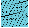
Pentagon1

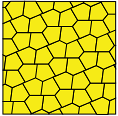
Pentagon2

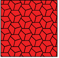
Pentagon3

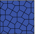
Pentagon4

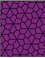
Pentagon5

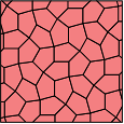
Pentagon8

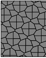
Pentagon10

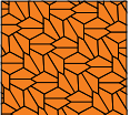
Pentagon11

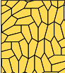
Pentagon15

 

Figure 2.3: The Pentagonal Tiling Variations Supported by Our Software
The images of these tilings are taken from the interactive demo provided by Ed Pegg [24]. The underlined pentagonal tiling variants shown above for special default settings of their implicit parameters are featured in the empirical pair correlation distributions shown in Figure A.5 (page A.5).

  

3 Pentagonal tilings of the plane

The constructions of the fifteen known distinct types of pentagonal tilings of the plane are one of the most famous problems in mathematics that has occupied mathematicians and housewives alike for most of the $20^{th}$ and $21^{st}$ centuries. One of Hilbert’s twenty-three open problems in mathematics published in $1900$ considers finding equations for a full set of distinct classes of pentagonal tilings that cover the plane. Hilbert’s $18^{th}$ problem is partially resolved by the fourteen types of pentagon tilings discovered by K. Reinhardt (1918), R. B. Kershner (1968), R. James (1975), M. Rice, and R. Stein (1985) throughout the twentieth century. The fifteenth known class of these famous pentagonal tilings was recently discovered by computer assisted researchers in $2015$. An exhaustive interactive demonstration of all fifteen of the pentagon tilings provided by the reference [24] shows the other variations including the nine tiling variants illustrated in Figure 2.3.

We have implemented a subset of these tilings in our software to perform statistics on the tile vertices of patches of the first, second, third, fourth, fifth, eighth, tenth, eleventh, and the most recent fifteenth pentagonal tilings in the forms of the default parameters to these tilings provided by the interactive demonstration mentioned above in Figure 2.3. Notice that these pentagonal tiling variants comprise the examples of non-substitution tilings provided by default in our software. We also provide a Sage worksheet for manipulating the statistical gap distribution plots of the newest fifteenth pentagonal tiling on our project website [27].

We analyze the plots of the pair correlation between these vertex sets in the comparisons given in the figures below. Side-by-side comparisons summarizing the empirical pair correlation between points in these tilings computed using our software is given in Figure A.5 (page A.5). The open-source software we provide on our website is easily modified to support other variations of these nine parameterized classes of pentagon tilings. To our knowledge, the results in the figures below provide the first computations of the gap and pair correlation distributions for these pentagonal tilings, and in particular, for the newest fifteenth pentagonal tiling recently discovered within the last two years.

4 Ulam sets in two dimensions

4.1 Definitions of Ulam sets and their geometric properties

We first recall the two-dimensional Ulam set construction introduced in §1.1.2. The next definitions make our intuitive definition of two-dimensional Ulam sets from the introduction and their key geometric properties more precise.

4.1.1 Ulam sets

Given two linearly independent initial vectors $v_{0},v_{1}\in\mathbb{R}_{\geq 0}^{2}$, define the Ulam set after $N:=0$ time steps to be

$$U_{0}:=\{v_{0},v_{1}\}.$$

We then construct subsequent stages of the Ulam set after $N\geq 1$ time steps recursively according to the formula

$$U_{N}=U_{N-1}\bigcup\left\{v+w:v\neq w\in U_{N-1}\text{ and }||v+w||=M_{N-1}\right\},$$

where

$$M_{N}:=\min\left\{||w_{1}+w_{2}||:w_{1},w_{2}\in U_{N},w_{1}\neq w_{2},w_{1}+w_{2}\neq w_{3}+w_{4}\text{ for any two pairs }w_{1}\neq w_{2},w_{3}\neq w_{4}\right\},$$

and where $||w||\equiv||w||_{2}$ denotes the two-norm, or Euclidean distance of the vector $w$ from the origin. That is, we define the Ulam set $U_{N}$ after $N$ timing steps to be the Ulam set $U_{N-1}$ together with the set of all vectors of minimal norm that can be uniquely written as the sum of two vectors in the previous set $U_{N-1}$. We let $U_{\infty}=\bigcup_{N\geq 0}U_{N}$.

4.1.2 The structure of the Ulam set points

The infinite set $U_{\infty}$ consists of points of the form $av_{0}+bv_{1}$ where $(a,b)=(n,1),(1,n)$ for some $n\in\mathbb{Z}_{\geq 0}$, or $(a,b)=(m,n)$ for some odd positive integers $m,n\geq 3$ [13, Thm. 1]. We also consider the sequence of $n^{th}$ line segments $L_{n}$ in the wedge spanned by $v_{0}$ and $v_{1}$ defined by

$$L_{n}=\{xv_{0}+yv_{1}:x,y\geq 0,x+y=n+1\}.$$

Geometrically, these $n^{th}$ line segments correspond to the negatively-sloped lines on the cross grains of the wedge defined by the vectors $(1,\varphi),(\varphi,1)$ in Figure 4.1. The number of Ulam set points on the $n^{th}$ line segment $L_{n}$ is given by

$$\#_{\operatorname{Ulam}}(n)=\begin{cases}2,&\text{ if $n$ is even; }\\ \frac{(n+1)}{2}&\text{ if $n$ is odd. }\end{cases}$$

As we will show in proving Theorem 4.1 in the next subsections, the $L_{n}$ form natural bins for the Ulam set points which are filled in approximately in order, as in $L_{n}$ before $L_{n+1}$, and so on. Thus we may construct so-termed “timing distributions” based on the intervals of time steps at which these $n^{th}$ bounded segments are filled by the vectors in $U_{N}$.

4.1.3 Representations of the vectors on the $n^{th}$ line segments

One central point to understanding the proof of Theorem 4.1 given below is to note the several different, but equivalent representations of the vectors on the constructions of the $n^{th}$ geometric line segments which are defined above. In particular, when $n$ is even the two vectors on $L_{n}$ are given by $nv_{0}+v_{1}$ and $v_{0}+nv_{1}$, and when $n$ is odd we have the following three key representations of the vectors on $L_{n}$ which result by symmetry in the representations involving $v_{0},v_{1}$:

$$av_{0}+bv_{1}, a,b\geq 1\text{ both odd, }a+b=n+1;$$ (I)

$$(n+1-b)v_{0}+bv_{1},bv_{0}+(n+1-b)v_{1}, b=1,3,5,\ldots,n$$ ; (II)

$$\frac{n+1-2d}{2}(v_{0}+v_{1})+2dv_{0},\frac{n+1-2d}{2}(v_{0}+v_{1})+2dv_{1}, \text{$d\in\left[-\frac{n-1}{2},\frac{n-1}{2}\right]$, }b\mapsto\frac{n+1}{2}-d.$$ (III)

4.1.4 Prototypical examples of the Ulam sets

We first consider the special cases of the Ulam set construction defined in the previous subsection corresponding to the initial vectors $\{v_{0},v_{1}\}:=\{(1,\varphi),(\varphi,1)\}$ and one case of an Ulam set arising from two non-parallel initial vectors chosen randomly from $[0,1]^{2}$. Figure 4.1 and Figure 4.2 provide the respective points in these two special infinite Ulam sets truncated after $N:=250$ steps of the recursive procedure used to generate successive points in the sets. Plots of the empirical slope gap and pair correlation distributions for two Ulam sets defined by the initial vector cases of $\{v_{0},v_{1}\}:=\{(1,\varphi),(\varphi,1)\}$ (as above) and the special case where $\{v_{0},v_{1}\}:=\{(1,0),(0,1)\}$ are compared in Figure A.6 on page A.6.

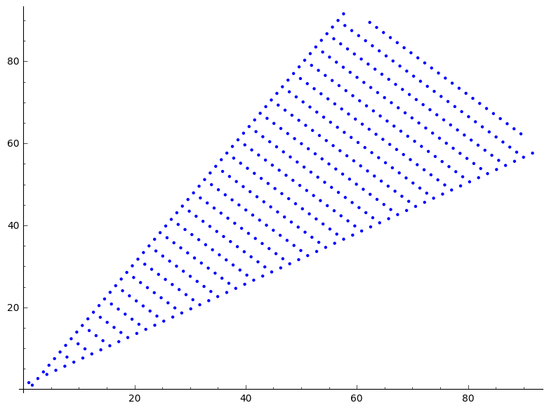
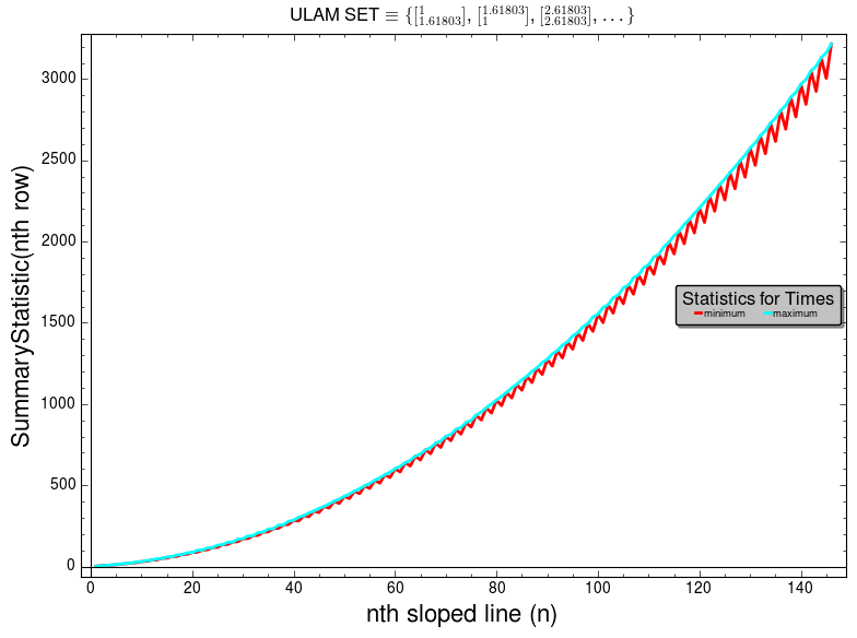
Figure 4.1: The Ulam set arising from $\{(1,\varphi),(\varphi,1)\}$ generated by running $ sage time-plots-random.sage userdef-2d 1 1.618034 1.618034 1 1500 with our software. The first image shows a plot of the Ulam set after $N:=250$ time steps. The second image shows the timing distribution of the maximum and minimum entry times of the Ulam set points on the $n^{th}$ line segments plotted over $n$ where the vectors involved in the timing plot correspond to the Ulam set after $N:=1500$ steps.

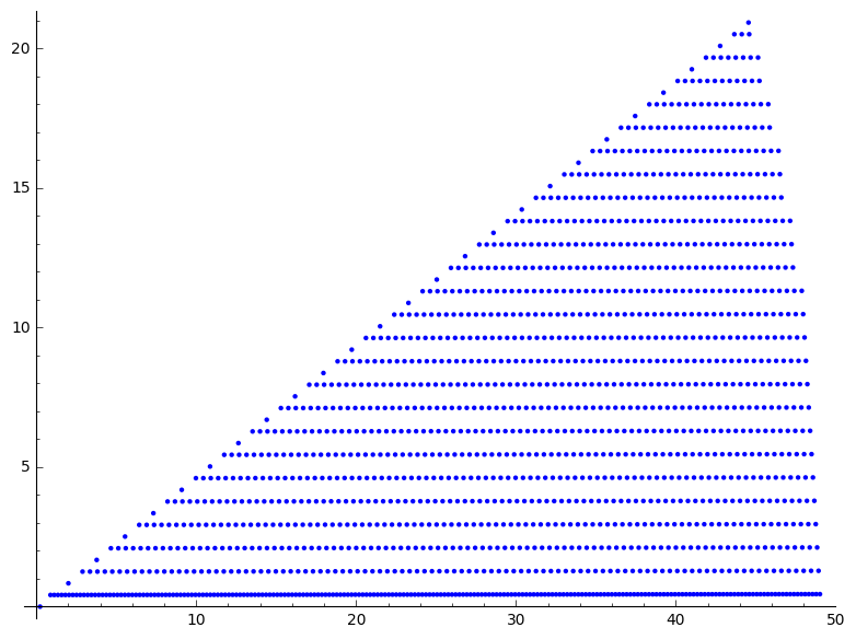
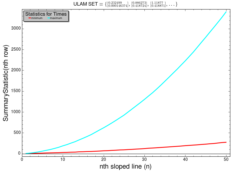
Figure 4.2: An Ulam set with randomly generated initial vectors in $[0,1]^{2}$ generated by running $ sage time-plots-random.sage random-2d 1500 with our software. The first image shows a plot of the Ulam set after $N:=1500$ time steps. The second image shows the timing distribution of the maximum and minimum entry times of the Ulam set points on the $n^{th}$ line segments plotted over $n$ where the vectors involved in the timing plot correspond to the Ulam set after $N:=1500$ steps.

4.2 Timing distributions of the generalized Ulam sets

4.2.1 An overview of timing properties in Ulam sets

We know both as a set definition and geometrically from the previous subsections what the points in the infinite Ulam sets correspond to as the number of steps $N\rightarrow\infty$ for some prescribed initial vectors, and moreover we see that these points are filled in gradually each over some fixed step $N<\infty$. It is then natural to ask questions about the timings of when Ulam set points at certain geometrical positions in the infinite set (or lattice points in the wedge defined by $v_{0}$ and $v_{1}$) formally enter the sets $U_{N}$. To the best of our knowledge such questions and conjectures relating to this subject matter have not yet been posed in the literature on generalized Ulam sets.

Plots of a subset of the timing summary statistics we consider in our Ulam sets source code for the two prototypical cases from the previous subsection are also provided in the bottom rows of Figure 4.1 and Figure 4.2 when the number of steps used to generated the Ulam set is $N:=1500$. The results and the proof of Theorem 4.1 given in the next subsection are essentially formulated in order to relate the number of steps $N$ to the vectors on each $L_{n}$, which are a priori distinct and unrelated parameters in the Ulam set construction.

4.2.2 A theorem on the timing distribution of minimum and maximum means

Theorem 4.1 (The Timing Distribution of the Maximum and Minimum Means).

If $T_{\max}(n)$ and $T_{\min}(n)$ denote the maximum and minimum entry times of the vectors on the $n^{th}$ line segment $L_{n}$, respectively, we have that there exist constants $C_{1},C_{2},C_{3},C_{4}>0$ such that for all sufficiently large $n$ we have that

$$C_{1}\cdot n^{2}\leq T_{\max}(n)\leq C_{2}\cdot n^{2}\quad\text{ and }\quad C_{3}\cdot n^{2}\leq T_{\min}(n)\leq C_{4}\cdot n^{2},$$

i.e., that there is a large $n_{0}\geq 1$ such that the inequalities above hold for all $n\geq n_{0}$. More precisely, if we define the maximum and minimum means of the entry times of the vectors on $L_{n}$ to be

$$T_{\max}(n) =\max\ \left\{N\geq 1:\text{some vector $w\in L_{n}$ satisfies }w\in U_{N}\text{ and }w\notin U_{N-1}\right\}$$

$$T_{\min}(n) =\min\ \left\{N\geq 1:\text{some vector $w\in L_{n}$ satisfies }w\in U_{N}\text{ and }w\notin U_{N-1}\right\},$$

then we have the tight asymptotic bounds on the growth of these two functions stated above: $T_{\max}(n)=\Theta(n^{2})$ and $T_{\min}(n)=\Theta(n^{2})$.

Remark 4.2 (Interpretations and Implications of the Theorem).

Thus we are able to obtain asymptotic estimates for the time steps at which the vectors $av_{0}+bv_{1}\in U_{\infty}$ (in the infinite Ulam set definition) enter the Ulam set by partitioning these points geometrically according to the $n^{th}$ line segments defined above to estimate the distribution of $K(a,b)$ on the $n^{th}$ line segment $L_{n}$, where we define $K(a,b)$ to be the value of the first step time $N$ where the vector $av_{0}+bv_{1}$ appears in the Ulam set $U_{N}$, but not in the set $U_{N-1}$. As it turns out, this is the most natural way to estimate the values in the timing plots in the figures without resorting to a much more complicated and chaotic two-parameter, three-dimensional plot timing construction for $K(a,b)$ where $a$ and $b$ are taken to be independent of one another.

The timings on the $n^{th}$ line segments are a natural way to consider the entry times of individual vectors in the set since the $n^{th}$ line segments are approximately filled in completely one right after the other as the step times $N\geq 1$ increase, as we shall soon see in Proposition 4.4 proved below. That is to say that the entry times of the vectors into the Ulam set are already naturally grouped into approximate time intervals by these line segments to begin with, so we simply estimate our timing statistics based on the points in these natural bins. A good heuristic explaining why we expect the asymptotic bound to be $\Theta(n^{2})$ is that the number of points in the wedge on the line segments $L_{k}$ for $k=1,2,\ldots,n$ is quadratic in $n$, where we expect to add at most a bounded constant of $O(1)$ points at each distinct step (see Lemma 4.5 below) for a total of approximately a quadratic number of time steps needed to fill in $L_{n}$ completely.

Lemma 4.3 (Minimum and Maximum Magnitude Vectors).

Given all points on the $n^{th}$ line segment $L_{n}$, the minimum most magnitude vector on the line segment is in the boundary set $\{nv_{0}+v_{1},v_{0}+nv_{1}\}$ when $n$ is even, is given exactly by $\frac{n+1}{2}(v_{0}+v_{1})$ when $n\equiv 1\pmod{4}$, and is given exactly by $\frac{n+3}{2}v_{0}+\frac{n-1}{2}v_{1}=\frac{n-1}{2}(v_{0}+v_{1})+2v_{0}$ when $n\equiv 3\pmod{4}$. For all $n\geq 2$ the two vectors of the greatest (and not necessarily equal) magnitudes on the $n^{th}$ line segment are in the set $\{v_{0}+nv_{1},nv_{0}+v_{1}\}$.

Proof.

It is obvious that when $n$ is even, we only have two points on the $n^{th}$ segment $L_{n}$, so both claims are trivially true in this case. In the remaining two cases when $n$ is odd we can prove the claims by considering inequalities for large $n$. For odd $n$, we can write all vectors on the $n^{th}$ line segment in the form of

$$w_{d}:=\frac{(n+1-2d)}{2}(v_{0}+v_{1})+2dv_{0},\ \text{ for some $d\in\left[-\frac{n-1}{2},\frac{n-1}{2}\right]$. }$$

The distinction between the two odd cases for $n$ modulo $4$ comes into play since when $n\equiv 1\pmod{4}$ there are an odd number of vectors on the $n^{th}$ line segment, and when $n\equiv 3\pmod{4}$ there are an even number of vectors on the $n^{th}$ line segment where we are essentially considering the middle-most vectors on the segment for our candidates for the minimum magnitude vectors on the segment.

Let $v_{0}:=(x_{0},y_{0})$, $v_{1}:=(x_{1},y_{1})$, and let $\vartheta_{001}$ denote the angle between the vectors $v_{0}$ and $v_{0}+v_{1}$. Suppose that $n\equiv 1\pmod{4}$. Then we have claimed that the minimum magnitude vector on the $n^{th}$ line segment is given by $w_{0}$. Since $x_{0},x_{1},y_{0},y_{1}\geq 0$ we can show that for large $n$ we have that $||w_{0}||\leq||w_{1}||$ and that $||w_{0}||\leq||w_{-1}||$. Now suppose that $d\geq 2$ and consider the differences of the magnitudes of the vectors $w_{d}$ and $w_{d+1}$:

$$||w_{d}||^{2} -||w_{d+1}||^{2}=\frac{(n+1-2d)^{2}}{4}||v_{0}+v_{1}||^{2}+4d^{2}||v_{0}||^{2}+2d(n+1-2d)||v_{0}||\cdot||v_{0}+v_{1}||\cos(\vartheta_{001})$$

$$\phantom{=\ }-\left[\frac{(n-1-2d)^{2}}{4}||v_{0}+v_{1}||^{2}+4(d+1)^{2}||v_{0}||^{2}+2(d+1)(n-1-2d)||v_{0}||\cdot||v_{0}+v_{1}||\cos(\vartheta_{001})\right],\$$

by the polarization identity

$$=(n-2d)||v_{0}+v_{1}||^{2}-4(2d+1)||v_{0}||^{2}-(2n-8d-2)||v_{0}||\cdot||v_{0}+v_{1}||\cos(\vartheta_{001})$$

$$<0,\ \text{ for $n$ large. }$$

So when we increase the $d\geq 2$ the magnitude of the corresponding vector increases in magnitude. Similarly, for $d\geq 0$ we can easily show that the difference $||w_{d}||-||w_{d-1}||<0$. Thus we have proved our result in the first case of odd $n$. A similar modified argument shows that the second statement is also true. The inequalities we have established for the minimum magnitude vector cases show that the two maximum magnitude vectors on the $n^{th}$ line segment for $n$ odd are $\{v_{0}+nv_{1},nv_{0}+v_{1}\}$. ∎

Proposition 4.4 (Order of Point Entry Times on the $n^{th}$ Line Segment).

For $n\geq 2$, the vectors on the $n^{th}$ line segment $L_{n}$ are filled in completely before the vectors in the $(n+1)^{th}$ line segment $L_{n+1}$ are filled in completely. The number of Ulam set points filled in on the $k^{th}$ segments $L_{k}$ for $k>n$ before the $n^{th}$ line segment is filled in completely is $O(n^{2})$.

Restatement: The proposition is restated in more formal notation as follows: For all $n\geq 2$ there exists a smallest time step $N\equiv N(n)$ such that $U_{N}\cap L_{n}=L_{n}$ but where $U_{N}\cap L_{n+k}\subsetneq L_{n+k}$ for all $k\geq 1$. Moreover, for each $n\geq 2$ and its minimal time step $N(n)$ we have that

$$\sum_{k\geq 1}|U_{N(n)}\cap L_{n+k}|=O(n^{2}).$$

Proof.

Let $n\geq 2$ be fixed. Since the maximum magnitude vector on the $n^{th}$ line segment is given by $v_{0}+nv_{1}$ (cf. Lemma 4.3), and we have that for all $k\geq 1$ the norms satisfy $||v_{0}+nv_{1}||_{2}<||v_{0}+(n+k)v_{1}||_{2}$, i.e., that

$$||v_{0}+nv_{1}||_{2}<||v_{0}+(n+1)v_{1}||_{2}<||v_{0}+(n+2)v_{1}||_{2}<\cdots,$$

we see that the first of the results stated above is true. By Lemma 4.3, to prove the second result we must bound the maximum $m$ of the minimums of each of the following sets by $O(n)$ where $m:=\max\{m_{14},m_{34},m_{02}\}$ in the notation below:

$$m_{14} :=\min\ \left\{k\in\mathbb{Z}^{+}:\left\lVert\frac{(n+k+1)(v_{0}+v_{1})}{2}\right\rVert-||v_{0}+nv_{1}||_{2}^{2}>0\text{ and }n+k\equiv 1\pmod{4}\right\}$$

$$m_{34} :=\min\ \left\{k\in\mathbb{Z}^{+}:\left\lVert\frac{(n+k-1)(v_{0}+v_{1})}{2}+2v_{0}\right\rVert-||v_{0}+nv_{1}||_{2}^{2}>0\text{ and }n+k\equiv 3\pmod{4}\right\}$$

$$m_{02} :=\min\ \left\{k\in\mathbb{Z}^{+}:||(n+k)v_{0}+v_{1}||_{2}^{2}-||v_{0}+nv_{1}||_{2}^{2}>0\text{ and }n+k\equiv 0\pmod{2}\right\}.$$

Then we have points in the later $k^{th}$ segments with $k>n$ for a maximum of $m$ incompletely filled line segments in the Ulam set where each of these segments is filled with $O(n)$ points. Thus to complete the proof we must show that $m=O(n)$. We illustrate our method for doing so by considering the third set case in the equations above. More precisely, if we let $v_{0}:=(x_{0},y_{0})$ and $v_{1}:=(x_{1},y_{1})$, we require that for some minimal $k\geq 1$ we have that

$$((n+k)x_{0}+x_{1})^{2}+((n+k)x_{0}+x_{1})^{2}-\left[(x_{0}+nx_{1})^{2}+(y_{0}+ny_{1})^{2}\right]>0.$$

When we reduce this inequality we see that the previous equation implies that $1\leq k\leq O(n)$. The other two cases follow similarly by computation. Hence the total number of points in the subsequent line segments is bounded by $m\cdot O(n)=O(n^{2})$. ∎

Lemma 4.5 (Upper Bound on the Number of Points Added at Step $N$).

For sufficiently large $N$, the maximum number of vectors added to the finite Ulam set at step $N$ is some bounded integer-valued constant, $C_{v_{0},v_{1}}$, which depends only on the inner angle of the wedge formed by the fixed initial vectors $v_{0},v_{1}$ in the first quadrant and the magnitudes of $v_{0},v_{1}$, i.e., we have that

$$\sup_{N\geq 1}\left(|U_{N}|-|U_{N-1}|\right)=C_{v_{0},v_{1}}<\infty,$$

exists and is finite for each fixed initial vector pair $(v_{0},v_{1})$.

Proof.

Suppose that at some step $N$, $w_{1}$ is a minimal length vector to be added to the Ulam set with minimal $y$-coordinate. We need to count and bound the number of Ulam set points on the quarter circle in the first quadrant of radius $||w_{1}||_{2}$ whose $y$ components are strictly larger than that of $w_{1}$. We start the proof with exact estimates of the magnitudes of two proposed vectors on this quarter circle (assuming for the sake of argument that there are multiple minimum length vectors at step $N$) and then proceed to consider the approximate and asymptotic bounds on the parameters defining these vectors.

If we suppose that our first minimal magnitude vector $w_{N}:=(n+1-b)v_{0}+bv_{1}$ at time step $N$ is of minimal $y$-coordinate, then we may bound our constant at time step $N$ by the number of integer solutions $(t,s)\in\mathbb{Z}^{2}$ with $t=0,1,2,\ldots,s$ to the equation

$$||(n+1-b)v_{0}+bv_{1}||_{2}=||(n+1+s-(b+t))v_{0}+(b+t)v_{1}||_{2},$$

i.e., the number of integer solution pairs to the equation

$$s^{2}||v_{0}||^{2}+t^{2}||v_{1}-v_{0}||^{2}+2st||v_{0}||\cdot||v_{1}-v_{0}||\cos(\vartheta_{0}-\vartheta_{01})=4||w_{N}||^{2}\cos(\vartheta_{w}-|\vartheta_{0}-\vartheta_{01}|),$$

which is easier said than done exactly. However, to count the number of solutions $s$ where $t\in[0,s]$, we note that we can alternately bound the number of times the quarter circle of radius $R:=||w_{N}||$ crosses a distinct line segment $L_{n+s}$, which leads to the upper bound of $4\cdot\#(s)$ since there is a square root in the previous equation and since the quarter circle may intersect each $L_{n+s}$ it crosses at most twice. We then estimate $\#(s)$ by considering three points on the quarter circle: 1) $P_{1}$: the intersection with the line between $v_{0}$ and $v_{0}+v_{1}$, i.e., the line parameterized by $v_{0}+\lambda_{0}(v_{0}+v_{1})$; 2) $P_{2}$: the intersection with the line $v_{1}+\lambda_{1}(v_{0}+v_{1})$; and 3) $P_{3}$: the point of longest distance from $v_{0}+v_{1}$ on the quarter circle, which we can intentionally overshoot by defining

$$P_{3}:=\frac{v_{0}+v_{1}}{||v_{0}+v_{1}||}\left(||v_{0}+v_{1}||+R\right).$$

Without loss of generality, we consider the distance between $P_{1}$ and $P_{3}$ and then divide through by the minimum of the magnitudes of $v_{0},v_{1}$ (the approximate distance between the $L_{n}$) to obtain the desired upper bound for the number of line segments crossed by the quarter circle. In this case, we have that

$$\lambda_{0}=\frac{\sqrt{R^{2}-||v_{0}||^{2}-2||v_{0}||\cdot||v_{0}+v_{1}||\cos(\vartheta_{0}-\vartheta_{10})}}{||v_{0}+v_{1}||},$$

where $\vartheta_{10}$ denotes the angle formed between the $x$-axis and the vector $v_{0}+v_{1}$. Then our upper bound on the constant $C_{v_{0},v_{1}}$ is given by

$$C_{v_{0},v_{1}}\leq\frac{8\left\|\frac{v_{0}+v_{1}}{||v_{0}+v_{1}||}\left(||v_{0}+v_{1}||+R\right)-\left(v_{0}+\lambda_{0}(v_{0}+v_{1})\right)\right\rVert}{\min\ \{||v_{0}||,||v_{1}||\}}\xrightarrow{n\longrightarrow\infty}\frac{8}{\min\ \{||v_{0}||,||v_{1}||\}}\left(||v_{0}+v_{1}||+||v_{0}||\right),$$

where we have included an additional factor of $2$ in the upper bound due to possible symmetry in the initial vectors which can lead to two vectors on the same line segment $L_{n+s}$ having the same minimal magnitude. ∎

Example 4.6.

To verify that our formula is in the ballpark of the expected largest constant, we plug-in our known prototypical vector case of $v_{0},v_{1}:=(1,0),(0,1)$ to the formula above and maximize with respect to $R$. This leads us to the estimate that

$$C_{v_{0},v_{1}} \leq\frac{8}{\sqrt{2}}\left\lVert(1,1)(R+\sqrt{2})-\left(\sqrt{R^{2}-3}+\sqrt{2},\sqrt{R^{2}-3}\right)\right\rVert$$

$$=\frac{8}{\sqrt{2}}\sqrt{\left(R-\sqrt{R^{2}-3}\right)^{2}+\left(R-\sqrt{R^{2}-3}+\sqrt{2}\right)^{2}}$$

$$\leq 8\sqrt{4+\sqrt{6}}\approx 20.3167,\text{ which occurs for $R:=\sqrt{3}$. }$$

Our empirical observations of this initial vector case place the constant at $C_{v_{0},v_{1}}=12$, so we see that we have obtained a realistic estimate for finite $N$ with this bound. If we require that $||v_{0}||,||v_{1}||\in[1,Q]$ for some bounded real $Q>1$, a requirement which we may impose by scaling, we can estimate that $C_{v_{0},v_{1}}\leq 24\cdot Q$ to obtain another upper bound on the number of vectors that can be added to an Ulam set at any prescribed time step $N$.

Proof of Theorem 4.1.

We begin by considering the maximum mean case where we determine exact bounds on the order of the function $T_{\max}(n)$ defined above over $n$. To reach the points in the $n^{th}$ line segment for $n\geq 2$ we have a finite number of vectors in the $k^{th}$ previous line segments to cover for $0\leq k<n$. By Proposition 4.4 we have that there are $2$ points on the $k^{th}$ line segment if $k$ is even and $(k+1)/2$ points on the $k^{th}$ line segment if $k$ is odd.

Upper Bound Estimate on $T_{\max}(n)$: In the worst case analysis, we assume that we only add one vector to the finite Ulam set at each step $N$ and that the number of vectors filled in on the $k^{th}$ segments for $k>n$ when the last vector is filled in is bounded by $O(n^{2})$ according to Proposition 4.4. Then to reach the last vector on the $n^{th}$ segment, by the proposition it takes $N$ steps where

$$N_{n} =\sum_{k=0}^{n-1}\#_{\operatorname{Ulam}}(k)+\begin{cases}2&\text{ if $n$ is even; }\\ \frac{n+1}{2}&\text{ if $n$ is odd. }\end{cases}+O(n^{2})$$

$$=\sum_{k=0}^{\left\lfloor\frac{n-1}{2}\right\rfloor}2+\sum_{k=0}^{\left\lfloor\frac{n-1}{2}\right\rfloor}\frac{k+1}{2}+\begin{cases}2&\text{ if $n$ is even; }\\ \frac{n+1}{2}&\text{ if $n$ is odd. }\end{cases}+O(n^{2})$$

$$=\frac{1}{4}\left(\left\lfloor\frac{n-1}{2}\right\rfloor+1\right)\left(\left\lfloor\frac{n-1}{2}\right\rfloor+10\right)+\begin{cases}2&\text{ if $n$ is even; }\\ \frac{n+1}{2}&\text{ if $n$ is odd. }\end{cases}+O(n^{2})$$

$$=O(n^{2}).$$

Lower Bound on $T_{\max}(n)$: In the best case analysis, we have by Lemma 4.5 that we can add at most constant $C_{v_{0},v_{1}}$ number independent of $N$ and $n$ of vectors to the growing finite Ulam set at each step $k$ for $k\geq N_{0}\geq 1$, where we may assume for the sake of obtaining a lower bound that the $n^{th}$ line segment is filled in completely before any points on the $k^{th}$ line segments for $k>n$. Thus to reach the last vector on the $n^{th}$ segment in this case we require $N$ steps where

$$N_{n} \geq\sum_{k=N_{0}}^{n-1}O\left(\frac{\#_{\operatorname{Ulam}}(k)}{C_{v_{0},v_{1}}}\right)+\begin{cases}O\left(\frac{2}{C_{v_{0},v_{1}}}\right)&\text{ if $n$ is even; }\\ O\left(\frac{n+1}{2C_{v_{0},v_{1}}}\right)&\text{ if $n$ is odd. }\end{cases}=O(n^{2}).$$

Hence $T_{\max}(n)=\Theta(n^{2})$. The computation for the minimum mean case is similar. ∎

5 Conclusions

We hope that this collection of data on tiling statistics and suggestions of theoretical methods to compute limiting distributions inspires further study in this area. We believe new methods will be needed to study many of the tilings, particularly those without obvious symmetries (or hidden symmetries in the case of quasicrystals). The tilings project website provides forms for interactive side-by-side comparisons of our plot data beyond the similarities between related tilings we suggest in this article. Our data is publicly available and freely usable, however, we do request that any use of the data cites this work and the website where the data is hosted.

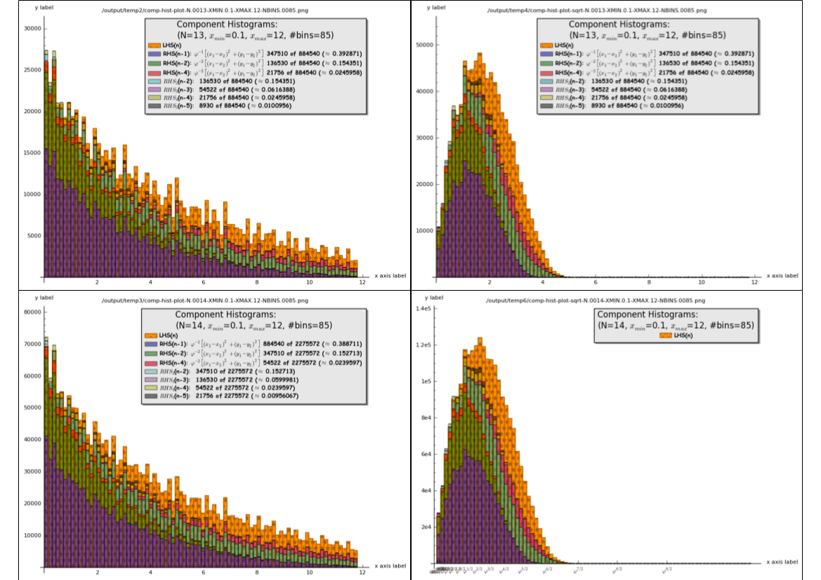
Figure A.1: Stacked Pair Correlation Plots for $N:13$ and $N:=14$. Key: Orange = Full Distribution (for visual comparision), Blue = $\operatorname{RHS}(n-1):=\varphi^{-1}\widetilde{D}_{n-1}$, Green = $\operatorname{RHS}(n-2):=\varphi^{-2}\widetilde{D}_{n-2}$, Red = $\operatorname{RHS}(n-4):=\varphi^{-4}\widetilde{D}_{n-4}$, Turquoise = $\operatorname{RHS}_{2}(n-2)$, Pink = $\operatorname{RHS}_{3}(n-3)$, Yellow = $\operatorname{RHS}_{4}(n-4)$, and Gray = $\operatorname{RHS}_{5}(n-5)$.

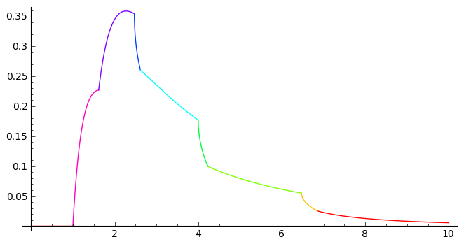
The piecewise smooth empirical distribution for the slope gaps of saddle connections on the golden L (vectors of slope at most $1$ and horizontal component less that $10^{4}$).

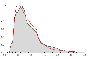
Empirical distribution of the slope gaps of the points in a long patch of the TubingenTriangle tiling (approximately $1.5\times 10^{6}$ points). The red comparision curve corresponds to Hall’s distribution for the slope gap distribution of the two-dimensional integer lattice.

Figure A.2: Empirical slope gap distributions for the SaddleConnGoldenL and TubingenTriangle tilings (permission to reproduce the second image from [5] given by T. Jakobi)

Figure A.3: Empirical slope gap distribution of the AmmannChair tiling after $N:=21$ substitution steps

 

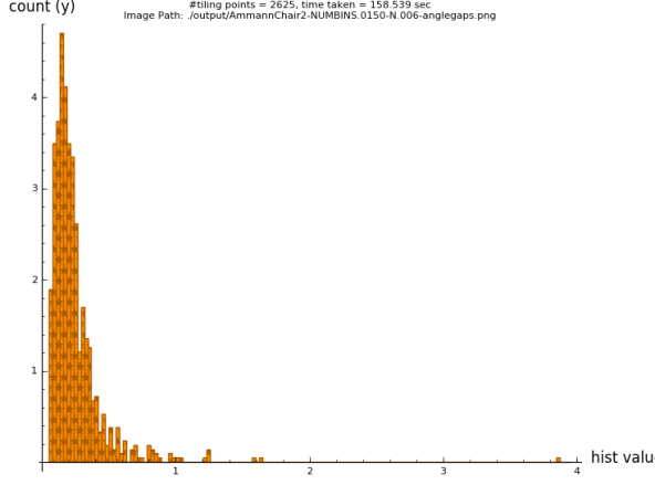
AmmannChair2 Angle Gaps

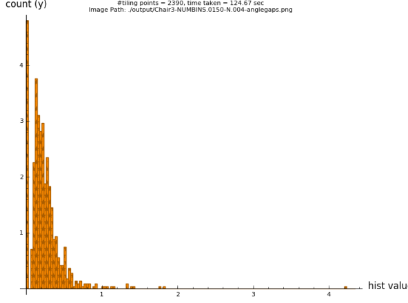
Chair3 Angle Gaps

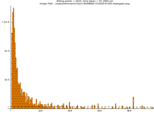
AmmannChair2 Slope Gaps

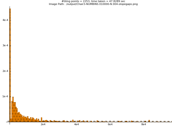
Chair3 Slope Gaps

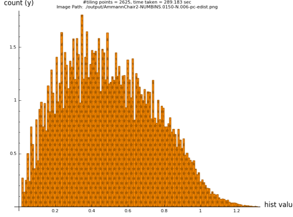
AmmannChair2 Pair Correlation

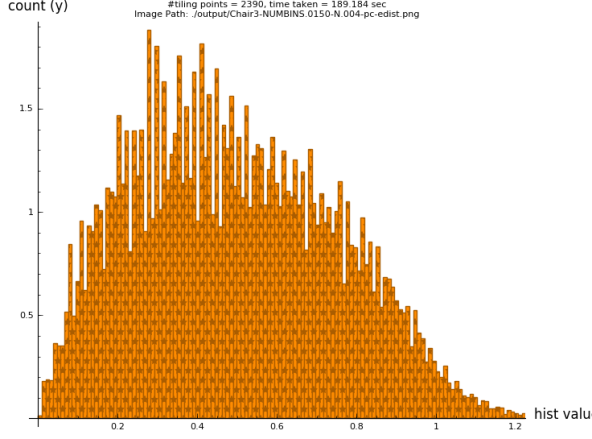
Chair3 Pair Correlation

Figure A.4: A Comparision of the Empirical Distributions of the AmmannChair2 ($N:=6$) and the Chair3 ($N:=4$) Tilings

 

 

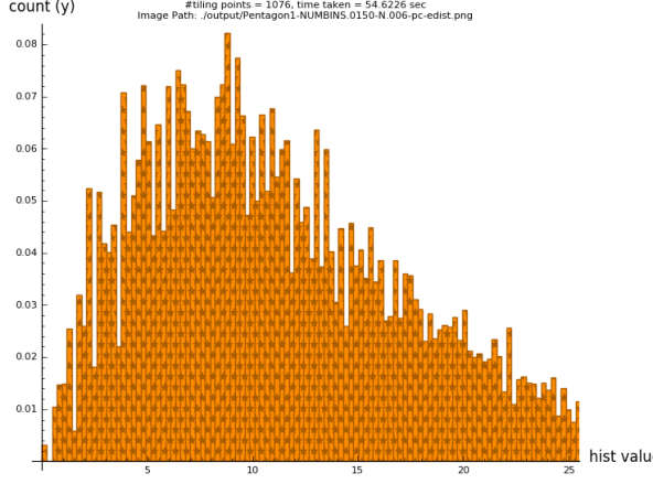
Pentagon1 Pair Correlation

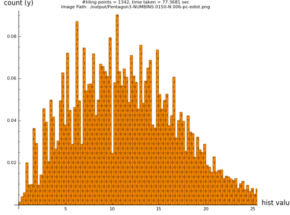
Pentagon3 Pair Correlation

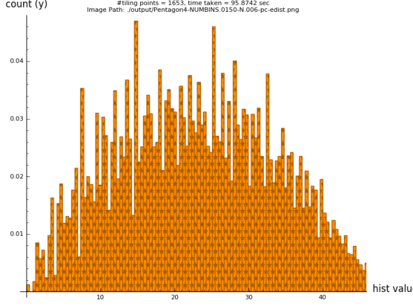
Pentagon4 Pair Correlation

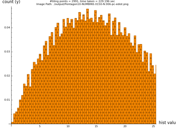
Pentagon10 Pair Correlation

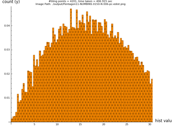
Pentagon11 pc-edist

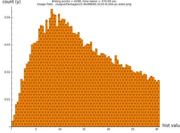
Pentagon15 Pair Correlation

Figure A.5: A Comparison of the Pair Correlation Plots for a Subset of the Pentagon Tilings

 

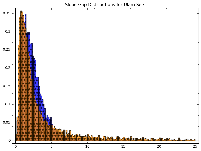
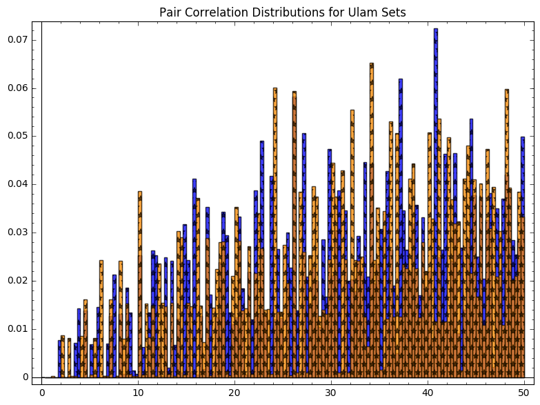
Figure A.6: A Comparison of the slope gap and pair correlation empirical distributions where the slope gaps are scaled by a factor of the wedge angle between $v_{0},v_{1}$ for $v_{0},v_{1}=(0,1),(1,0)$ (orange) and $v_{0},v_{1}=(1,\varphi),(\varphi,1)$ (blue) when $N:=5000$

References

- [1] J. S. Athreya, Gap distributions and homogeneous dynamics. Proceedings of ICM Satellite Conference on Geometry, Topology, and Dynamics in Negative Curvature, 2016.
- [2] J.S. Athreya, J. Chaika, The distribution of gaps for saddle connection directions. Geometric and Functional Analysis,Volume 22, Issue 6, 1491-1516, 2012.
- [3] J. S. Athreya, J. Chaika, S. Lelievre, The gap distribution of slopes on the golden L. Contemporary Mathematics, volume 631, 47-62, 2015.
- [4] J. S. Athreya, Y. Cheung, A Poincaré section for horocycle flow on the space of lattices. International Mathematics Research Notices, Issue 10, 2643-2690, 2014.
- [5] M. Baake, F. Götze, C. Huck, and T. Jakobi, Radial spacing distributions from planar points sets, 2014, https://arxiv.org/abs/1402.2818.
- [6] M. Baake and U. Grimm, Mathematical diffraction of aperiodic structures, Chem. Soc. Rev. 41 (2012) 6821-6843
- [7] F. Boca, C. Cobeli, and A. Zaharescu, A conjecture of R. R. Hall on Farey points. J. Reine Angew. Math. 535 (2001), 207 - 236.
- [8] F. P. Boca and A. Zaharescu, Farey fractions and two-dimensional tori, in Noncommutative Geometry and Number Theory (C. Consani, M. Marcolli, eds.), Aspects of Mathematics E37, Vieweg Verlag, Wiesbaden, 2006, pp. 57-77.
- [9] N.D. Elkies and C.T. McMullen, Gaps in mod 1 and ergodic theory. Duke Math. J. 123 (2004), 95-139.
- [10] Grimm, Uwe and Schrieber, Michael, Aperiodic Tilings on the Computer, Quasicrystals, Volume 55, Springer Series in Materials Science pp 49-66, 2002.
- [11] B. Grünbaum and G. C. Shephard, Tilings and Patterns, Dover, 2016.
- [12] R. R. Hall, A note on Farey series. J. London Math. Soc. (2) 2 1970 139 - 148.
- [13] N. Kravitz and S. Steinerberger, Ulam sequences and Ulam sets, 2017, https://arxiv.org/abs/1705.01883.
- [14] J. Marklof and A. Strömbergsson, The distribution of free path lengths in the periodic Lorentz gas and related lattice point problems. Ann. of Math. (2) 172 (2010), no. 3, 1949–2033
- [15] J. Marklof and A. Strömbergsson, Free path lengths in quasicrystals. Comm. Math. Phys. 330 (2014), no. 2, 723-755
- [16] E. A. Robinson, Jr., On the table and the chair. Indag. Mathem., N.S., 10 (4), pp. 581-599, 1999.
- [17] L. A. Sadun, Topology of tiling spaces. American Methematical Society (2008).
- [18] S. Steinerberger, A hidden signal in the Ulam sequence, 2016, https://arxiv.org/abs/1507.00267.
- [19] C. Uyanik and G. Work, The distribution of gaps for saddle connections on the octagon, International Math Research Notices (2015).
- [20] G. Work, Transversals to horocycle flow on H(2), preprint.
- [21] Two-dimensional geometry and the Golden section, 2016, http://www.maths.surrey.ac.uk/hosted-sites/R.Knott/Fibonacci/phi2DGeomTrig.html.
- [22] Non-periodic substitution tilings, 2016, http://blog.wolframalpha.com/2011/07/15/non-periodic-substitution-tilings/.
- [23] Wolfram demonstrations project: Ammann chair, 2016, http://demonstrations.wolfram.com/AmmannChair/.
- [24] Wolfram demonstrations project: Pentagon tilings, 2016, http://demonstrations.wolfram.com/PentagonTilings/.
- [25] Wolfram demonstrations project: Ammann tiles, 2016, http://demonstrations.wolfram.com/AmmannTiles/.
- [26] Tilings Encyclopedia, 2016, http://tilings.math.uni-bielefeld.de/.
- [27] Tiling gap distributions and pair correlation project, 2016, http://www.math.washington.edu/wxml/tilings/index.php.