Plunges in the Bombay Stock Exchange: Characteristics and Indicators

Abstract

We study the various sectors of the Bombay Stock Exchange(BSE) for a period of 8 years from January 2006 - March 2014. Using the data of daily returns of a period of eight years we investigate the financial cross-correlation co-efficients among sectors of BSE and Price by earning (PE) ratio of BSE Sensex. We show that the behavior of these quantities during normal periods and during crisis is very different. We show that the PE ratio shows a particular distinctive trend in the approach to a crash of the financial market and can therefore be used as an indicator of an impending catastrophe. We propose that a model of analysis of crashes in a financial market can be built using two parameters (i) the PE ratio (ii) the largest eigenvalue of the cross-correlation matrix(LECM).

I Introduction

The stock market is an extremely complex system with various interacting components Mantegna99 . The movement of stock prices are somewhat interdependent as well as dependent on a wide multitude of external stimuli like announcement of government policies, change in interest rates, changes in political scenario, announcement of quarterly results by the listed companies and many others. The overall result is a chaotic complex system which has so far proved very difficult to analyze and predict. However, with so much capital invested in the financial markets, a collapse in financial markets has the potential to cause widespread economic disruption. As an example, the market crash of 1929 was a key factor in causing the great depression of the 1930s depression1929 .

It is therefore of crucial importance to be able to predict such catastrophic events so that precautions and corrective steps can be taken. There has been an increased interest in studying and understanding the financial markets with Random Matrix Theory proving to be an useful tool (see RMT and references therein). It was observed that before stock market crashes, there was very high rise in the stock price without high increase in earning Galbraith . This pattern was present in almost all great crashes Foster . Currently, however we do not have any accepted model characterizing the collapse of a stock market Frankel . In fact there is no specific definition of what characterizes a crash predictcrash although log-periodic power law singularity (LPPLS) models Sornette are promising candidates. A first step towards studying and modeling behavior of markets before and during a crash would be to find what are the characteristics of a crash, i.e. to identify and study which market parameters show distinctive behavior during the time when a financial market collapses.

It is well known that the market becomes very highly correlated during any period of high volatility volatility but it is not clear whether any such period of high correlation can be considered to be a crash. In this paper we try to analyze this question and offer tentative proposal of a procedure to predict a crash in the financial market. To identify such market parameters, we study the data of the daily returns of 12 sectors of the BSE for about $2000$ days from beginning of January 2006 to end of March 2014 BSE .

To understand and analyze the data we look at the logarithmic returns of the market. If $P_{i}(t)$ is the index of the sector $i=1,\dots,N$ at time $t$, then the (logarithmic) return of the $i$th sector over a time interval $t=1$ to $t=T$ days in the interval is defined as

$$R_{i}(t)\equiv\ln{P_{i}(t)}-\ln{P_{i}(t-1)}$$ (1)

For our data, $T=1900$, the number of days we have considered, and $N=13$ because we look at the following 12 sectors S$\&$P BSE Auto (Auto), S$\&$P BSE Bankex (Bankex), S$\&$P BSE Consumer Durables (CD), S$\&$P BSE Capital Goods (CG) , S$\&$P BSE FMCG (FMCG), S$\&$P BSE Health care (HC), S$\&$P BSE IT (IT), S$\&$P BSE Metal (Metal), S$\&$P BSE Oil and Gas (Oil and Gas), S$\&$P BSE Power (Power), S$\&$P BSE Realty (Realty) and S$\&$P BSE Teck (Teck) and the S$\&$P BSE SENSEX (Sensex) which serves as the benchmark. We will be treating each sector as one entity in the rest of the paper.

Volatility is a statistical measure of the dispersion of returns for a given security or of a market index. If $R_{i}$ is the return and $\mu_{i}$ is the return for the $i$th sector averaged over one month window respectively, we can define volatility of the $i$th sector over a certain period of time $T_{s}$ as

$$\sigma_{i}(T_{s})=\sqrt{\frac{1}{T_{s}}\sum_{t=1}^{T_{s}}\left(R_{i}(t)-\mu_{i}\right)^{2}}$$ (2)

In the context of our data, $T_{s}$ will be one month. It is known that high volatility of a market is linked to strong correlations among it’s sectors, i.e., sectors tend to behave as one during a crash volatility2 . In this paper we do a model independent quantitative study of the parameters which capture this feature.

To study the correlations between the sectors we construct the monthly correlation matrix whose entries are given by

$$C_{ij}=\frac{\left<(R_{i}-\mu_{i})(R_{j}-\mu_{j})\right>}{\sqrt{(\left<R^{2}_{i}\right>-\mu^{2}_{i})(\left<R^{2}_{j}\right>-\mu^{2}_{j})}}$$ (3)

where, as before, $R_{i}$ is the return and $\mu_{i}$ is the average return for the $i$th sector respectively. The averaging is done over a month. We will study the time evolution of this correlation matrix, i.e. study the monthly variation of some of the properties of the correlation matrix. Note that, unlike the analysis in ourpaper1 , we will mainly be focussing on periods of time when the crisis in the market occurred and compare it with the behavior during normal times. Our goal in this paper is to identify characteristics during these periods which were quantitatively different from those during the the normal periods. These parameters can be used to identify, characterize and model crashes in the future.

Apart from the behavior of correlations, in this paper we also explore the behavior of another important parameter, the Price by Earning (PE) Ratio PEratio1 . In the period under consideration, although there have been several events of high volatility and high fluctuations, two major events can be termed as crash Blankenburg : (i) financial crisis (May 2006) and (ii) recession in the US (Jan 2008). We shall call periods of high volatility as crisis periods in this paper while the term crash will be reserved only for the two periods mentioned above, when the global financial markets collapsed. Some work in this direction has been undertaken in crashbehav . The novelty in our work is that we simultaneously study the correlations in the stock market and the PE ratio and observe that both need to be high for the financial markets to crash. A systematic study of both the parameters and their behavior in the lead up to a crash has not been performed before (at least in the context of Indian markets) to the best of our knowledge.

Our paper is organized as follows: In section (II) we study the properties of the correlation matrix and identify characteristics which were quantitatively different during the crisis periods and the normal periods. We show that this feature can also be captured very elegantly using the cross correlation matrix between sectors. In section (III) we study the behavior of the PE ratio before, during and after the two crashes of the stock market mentioned above. We study the variation of the PE ratio and show that it can be one of the most important indicators of a crash. Further, from the analysis of the data we propose that it is possible to study, analyze and intensity of a market crash using two very important parameters Toth , the PE ratio and the largest eigenvalue of the correlation matrix(LECM). We finally end with our conclusions and observations in section (IV).

II Properties of the Correlation Matrix

To understand a period of high volatility, we first need to determine which features of the correlation matrix Plerou may be of interest during that period. The high volatility of the financial market is related to eigenvalues of a correlation matrix. The largest eigenvalue of a correlation matrix (LECM) often becomes very large compared to other eigenvalues(e.g. second and third largest eigenvalues) of the correlation matrix during high volatility period. Hence this feature is quantified using the correlation matrix. In all the figures in this section, the periods of high volatility will be marked out in grey. They correspond to

• May - July 2006

• July - September 2007

• January - March 2008

• August - December 2008

Note that, high volatility always leads to a large value of LECM but the converse is not true. A large value of LECM does not necessarily indicate high volatility.

Choosing some value of a threshold $t$, the correlation matrix is converted to the adjacency matrix, that is, if $C_{ij}\geq t$ the corresponding entry in the adjacency matrix is $1$ and $0$ otherwise. The number of connections i.e. the connectedness gives a measure of the amount of correlations existing in the market in a given month. The variation of connectedness of the 12 sectors and sensex with time can be seen in Figs.(1)and (2) for $t=0.9$ and for $t=0.85$. As can be seen from these two figures, the inclusion of the sensex along with the 12 sectors does not change the variation of the connectedness with time. Therefore in all the subsequent analysis of the features of the correlation matrix we have included the sensex along with the 12 sectors.

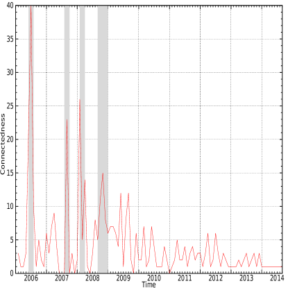
(a) Connectedness with $t=0.90$

(b) Connectedness with $t=0.85$

Figure 1: Variation of connectedness of the 12 sectors and sensex with time

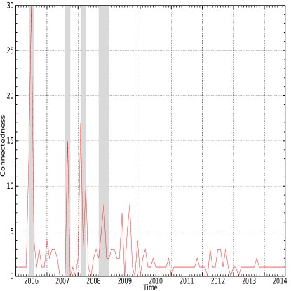
(a) Connectedness with $t=0.90$

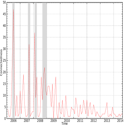
(b) Connectedness with $t=0.85$

Figure 2: Variation of connectedness of the 12 sectors with time

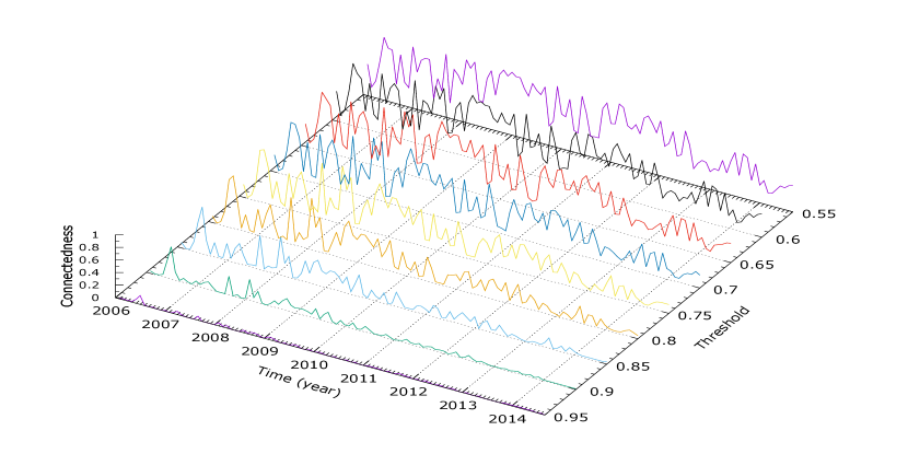
Figure 3: (Normalized) Connectedness with $t=0.95$, $t=0.90$, $t=0.85$, $t=0.80$, $t=0.75$ and $t=0.75$

Although the choice of threshold is arbitrary it does not change the conclusions. As can be seen from Figs.(1), (2) and (3), the qualitative features do not change with changing $t$ but obviously the actual nature of the connectedness becomes more apparent above some value of the threshold. For convenience the value of $t=0.9$ can be chosen so that the number of connections during normal periods is below 10 but increases significantly during periods of high volatility. It is also evident from these figures that correlation among sectors are quite high during crisis period and low in normal period. It is obvious that during periods of financial crisis (the grey regions in the figure) the market is highly correlated and hence strongly connected.

We further illustrate this feature by constructing a graph from the adjacency matrix of $t=0.9$ in Fig.(4) for two representative months. In the graph, each sector is represented as a node. Two nodes are connected by a link if the corresponding entry in the cross correlation matrix is above the threshold $t=0.9$. It can be clearly seen that during crisis periods (eg. April 2006) the resultant graph is highly connected with almost all the sectors linked to each other. That is not the case during normal periods (eg. May 2010) when the numbers of links are much less.

(a) During crisis period (April 2006)

(b) During normal period (May 2010)

Figure 4: Comparison of connectedness during a crisis and normal periods

Another way to characterize periods of crisis is to look at the mean, standard deviation and the ratio of standard deviation to mean of the correlation matrix in Fig.(5).

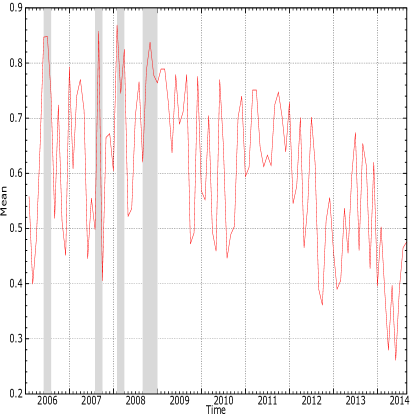
(a) Mean value of the correlation matrix with time

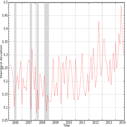
(b) Standard Deviation of the correlation matrix with time

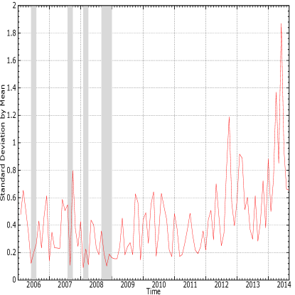
(c) Ratio of Standard Deviation to Mean of the correlation matrix with time

Figure 5: Variation of Mean, Stdev. and Stdev.to Mean with time

Periods of high mean correlation and low standard deviation signify a highly correlated market volatility3 . During normal periods the mean is around or below 0.80 and during a crisis, the value is above 0.80 such as in April 2006 when it touched 0.85. Similarly, during normal periods the standard deviation is around or above 0.12 and during a crisis, the value is much lower such as in April 2006 when it dropped to 0.10. Similar features can be seen in the ratio of standard deviation and mean.

Some of the individual entries of the correlation matrix also contain information about large volatility Iori . A relatively large value of minimum correlation suggests that sectors that would otherwise not be related, are moving together. As can be seen in Fig.(6) during normal periods its value is a way below 0.65 and during a crisis the value is above 0.65.

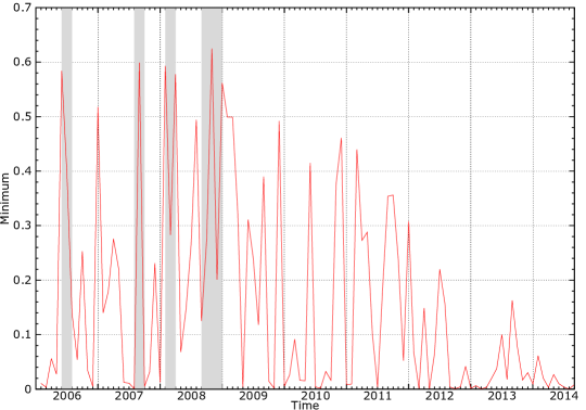
(a) Smallest element of the correlation matrix

Figure 6: Variation of Minimum Correlation

Another good measure of the correlation existing in the market can be obtained from studying the largest eigenvalue of the correlation matrix of the 12 sectors and sensex. We shall denote the largest eigenvalue of the correlation matrix as LECM subsequently. The largest eigenvalue of a correlation matrix indicates the maximum amount of the variance of the variables which can be accounted for with a linear model by a single underlying factor Friedman1981 . A large value is an indicator of a common driving force behind the entire market volatility4 . This is especially relevant during a crisis. From Figs.(7), we can see that during normal periods the largest eigenvalue is below 10 and during a crisis the value is closer to 11. We can also see clearly from Fig.(8) that second and third largest eigenvalues of the correlation matrix of 12 sectors and sensex are low during crisis periods but are quite high during normal periods.

Note that, as expected Friedman1981 , the graph for the mean value of the correlation matrix (Fig.(5a)) and that of the largest eigenvalue of the correlation matrix (Fig.(7) is qualitatively similar. However we choose to work with largest eigenvalue instead of the mean value of correlations because it is more connected to Random Matrix Theory. Subsequently, in this paper, we use LECM to capture the presence of high correlations in the financial market.

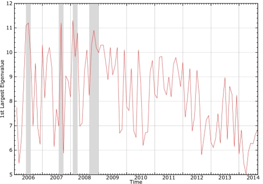
Figure 7: Largest eigenvalue of the correlation matrix

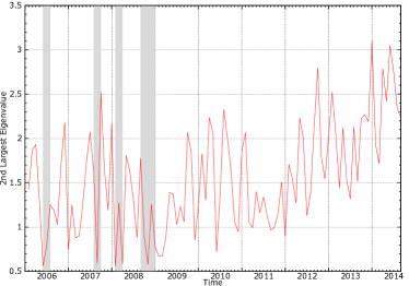
(a) Second Largest Eigenvalue

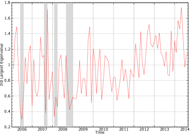
(b) Third Largest eigenvalue

Figure 8: Second and Third largest eigenvalue of the correlation matrix

Therefore we can argue that any crisis period of a stock market can therefore be characterized by the following properties

• high volatility

• high connectedness among sectors

• low standard deviation of correlations

• high mean correlation

• high maximum correlation

In all the figures above, the grey regions denote periods of high volatility. These periods can be checked against historical data of SENSEX ( see Table (1)) to justify our assertion from the table.

Period	Closing Index (min)	Closing Index (max)	Remark
May-July 2006	8929.44	12612.38	three consecutive large fall (May 18, 19, 22)
July- Sept 2007	13989.11	17291.1	no consecutive large fall
Jan- March 2008	14809.49	20873.33	three consecutive large fall (Jan 18, 21, 22)
Aug-Dec 2008	8451.01	15503.92	large fall but no consecutive fall

Table 1: Historical Data (SENSEX)

Note that our analysis is done with monthly averages and consequently our results will only indicate high volatility periods which lasted at least more than a month.

III Major Plunges in BSE

In this section, we will explore the behavior of the PE ratio(PE) for the period under consideration. Let us first qualitatively explain why we expect the PE ratio to be a significant indicator of a upcoming crisis. Most of the crashes of the financial markets are part of the boom and bust cycle which is captured by the PE ratio PEratio1 ; PEratio2 . Note that, earnings, book value and dividend for each stock is assumed to be constant for each quarter and only change when the next quarterly results are announced. In the absence of any external news the price fluctuation of a stock will be almost random over a quarter. If however the market sentiment is positive and external factors indicate that the next quarter results will show increased earning, the movement trend of the stock price will be in the upward direction. If this sentiment continues for longer time, the rate of increase of the stock price will rise faster than the rate of increase based on the expected increase of earnings. Owing to correlations present in the market, this will cause the upward movement of other stocks thereby increasing the PE ratio. If the positive sentiment sustains for longer period, the PE ratio will become very high. Consequently the market will become unsustainable. Note that, during this period the market movement cannot be explained on the basis of the quarterly results on earnings and book values. A continuous stream of external good news affect the market and there are more buyers than sellers. The imbalance due to consistent good news drives the market to new high for some times. This state of the market is a very unstable equilibrium which can be disturbed by a stream of bad news. Thereafter the market crashes and normalcy is established again PEratio3 . In Fig. (9) we plot the variation of the PE ratio over time while Fig (10.a) gives the variation of both the LECM (of the 12 sectors and the sensex) and the PE ratio over time.

Therefore the PE ratio can be used as a measure of the unsustainability of the market while the LECM can be used to measure how much the market as a whole is susceptible to external news Lilo . For a given (high) value of LECM and same intensity of negative external news, a market with very high PE ratio is more likely to crash than the market with low PE ratio.

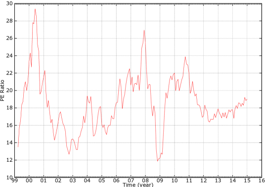
Figure 9: Variation of PE Ratio over time

The analysis of LECM was done in the previous section (see Fig. (7)). From historical data we know that there have been two major crashes in the BSE in this time period (i) May 2006 (ii) January 2008. A consistently high monthly PE ratio of sensex (25 $\pm$ 5) and high LECM ($\geq 11$) is a signature of highly non-equilibrium market leading to a crash. In Tables (3, 3 ) we see the variation of the PE ratio and the largest eigenvalue of the correlation matrix (LECM) before, during and after these two events.

Month	LECM	PE Ratio of Sensex
Jan 06	7.75	18.6
Feb 06	5.46	18.64
Mar 06	6.4	20.04
Apr 06	8.68	21.35
May 06	11.05	20.41
Jun 06	11.2	17.9

Table 2: Around May 2006

Month	LECM	PE Ratio of Sensex
Oct 07	9.04	24.86
Nov 07	8.83	25.44
Dec 07	8.17	26.94
Jan 08	11.32	25.53
Feb 08	9.82	22.23
Mar 08	10.76	20.18
Apr 08	6.98	20.71
May 08	7.11	20.66
Jun 08	9.25	18.22

Table 3: Around Jan 2008

A high value of PE ratio indicates an unsustainable market while a high LECM indicates a higher likelihood for a fluctuation in one sector to affect the entire market. From the Fig. (10) and the data in Tables (3, 3) and Figures(11 and 12 ) we can make several comments:

• The PE ratio as well as LECM at the time of crash in May 2006 was lower than that in January 2008. Consequently the severity of the crash was lower in 2006.

• Unlike May 2006, the PE ratio of the Sensex was consistently higher for several months before the January 2008 crash. We can conclude that before 2006 crisis, the market was slightly away from normal, while before 2008 crisis the market was at very high non-equilibrium state.

• From Fig. (9) we can see that there were other occasions when the PE ratio was above 20 but from Fig. (7) we can see that LECM was low during those times and hence the market did not crash.

• In Fig. (10.b) we have plotted the parameter space of LECM and PE ratio. The data point marked in yellow circle is January 2008 when both LECM and PE ratio were high. That was the onset of the crisis and the market went free fall till November 2008. This is shown by the values in the red box.

Our conclusion can also be easily verified by looking at Figs (11 and 12) which lists out the PE ratio and LECM of the entire period of time under consideration.

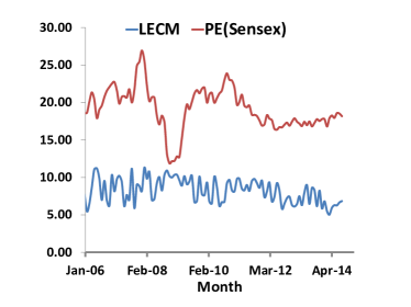
(a) Variation of LECM and PE ratio with time

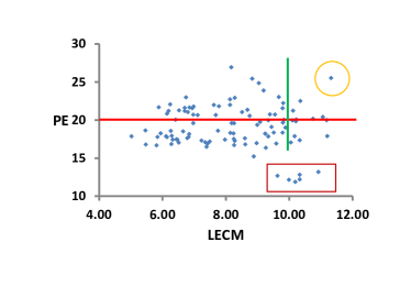
(b) Parameter Space of LECM and PE ratio

Figure 10: LECM and the PE ratio

Figure 11: Variation of LECM of 12 sectors with sensex and PE(Sensex) for period Jan 2006-Dec 2009

Figure 12: Variation of LECM of 12 sectors with sensex and PE(Sensex) for period Jan 2010-Apr 2014

To sum up, a large value of LECM means that almost all sectors are moving in the same direction. It seems natural that almost all sectors move in the same direction during large plunge period. This implies that we should have large principle eigenvalue during crisis period. This is confirmed by our analysis. Our study also shows that the converse is not true; we may get large principle eigenvalue sometimes during normal/high volatility periods. As the data shows, a large PE ratio is required along with a high LECM to push the market towards crash. In this paper, we show that a simultaneous study of LECM and PE ratio is a good indicator of a crash in the financial market. In fact, these may be used to also forecast a crash in the near future but the severity of the crash would depend on the prevailing market conditions Zhou ). Moreover the duration of the crash depends on how long the negative sentiment persists in the market, which, in turn, depends on the duration of the negative news.

IV Conclusions

The goal of this paper was to find indicators of a collapse of a stock market from studying the daily returns of BSE for 8 years. Let us emphasize once again that since our data set is the daily returns, all our statements pertain to periods of high volatility which lasted longer than a month at least. In particular, we will not be able to detect single day plunges of the stock market if it did not lead to (or was a part of) a sustained period of large volatility. With that caveat in mind let us briefly recapitulate what we have done.

It is well known that when unrealistic expectations of returns pushes the stock prices to extremely high values, the market corrects itself through a period of collapse. It is also well known that during a collapse of the market, the indices of all sectors go down irrespective of whether they were performing well or not. The first feature can be characterized by a high PE ratio while the second feature can be characterized by a high value of the largest eigenvalue of the cross correlation matrix (LECM). This indicates that studying the behavior of both these parameters, PE ratio and LECM, together may be a way of characterizing a crash.

That is exactly what we carry out in this paper. We show that by simultaneously studying the behavior of the PE ratio and LECM, we may actually determine the times when the crashes actually occurred. We also suggest that a consistent high value of the PE ratio along with a high LECM is a very strong indicator of an unstable market which is facing an impending collapse. One of the major advantages of our result is that it requires only two parameters for the prediction. This is expected to be of significant interest from the perspectives of portfolio management and economic policy decisions. It may also be of great value in future modelling of financial markets. However, this study has to be extended to other markets and other economies to strengthen the result. We also expect that the volume of shares traded may play a crucial role in studying crashes. This aspect, as well as a qualitative and quantitative study of some other market along the lines of the analysis carried out here is a direction of future work.

References

-
(1)
R. N. Mantegna and H. E. Stanley, “Introduction to Econophysics”, Cambridge University Press, Cambridge, (1999).
Sitabhra Sinha, Arnab Chatterjee, Anirban Chakraborti and Bikas K. Chakrabarti, “Econophysics: An Introduction”, Wiley-VCH, Weinheim, (2010). -
(2)
C. D. Romer, “What Ended the Great Depression”, The Journal of Economic History Vol 52, No. 4, (1992).
J. A. Tapia Granados and A. V. Diez Roux “Life and death during the Great Depression” PNAS Vol 106, No. 41, 17290–17295, (2009). -
(3)
V. Plerou, P. Gopikrishnan, B. Rosenow, L. A. Nunes Amaral, T. Guhr, and H. E. Stanley,
“Random matrix approach to cross correlations in financial data”, Phys. Rev. E 65, 066126 (2002).
H. Meng, W.J. Xie, Z.Q. Jiang, B. Podobnik , W.X. Zhou and H. E. Stanley, “Systemic risk and spatiotemporal dynamics of the US housing market”, Scientific Reports 4, Article number: 3655 (2014).
D.M. Song, M. Tumminello, W.X. Zhou, and R. N. Mantegna, “Evolution of worldwide stock markets, correlation structure, and correlation-based graphs”, Phys. Rev. E 84, 026108 (2011).
Y. H. Dai, W. J. Xie, Z. Q. Jiang, G.J.Jiang W. X. Zhou “Correlation structure and principal components in the global crude oil market”, Empirical Economics, 51.4, 1501-1519 (2016). -
(4)
J. N. Galbraith, “The Great Crash 1929”, Houghton Mifflin Harcourt, (2009).
R. Ball, “The Global Financial Crisis and the Efficient Market Hypothesis: What have we learned?.” Journal of Applied Corporate Finance 21.4 : 8-16 (2009).
D. Sornette, “Why Stock Markets Crash”, (Princeton Univ Press, Princeton NJ, 2003) - (5) J. B. Foster and F. Magdoff, “The Great Financial Crisis: Causes and Consequences” NYU Press, (2009).
- (6) J. Frankel and G. Saravelos, “Can Leading Indicators Assess Country Vulnerability? Evidence from the 2008–09 Global Financial Crisis” Journal of International Economics 87.2 : 216-231 (2012).
- (7) M. S. Focardi and F. J. Fabozzi, “Can We Predict Stock Market Crashes?” The Journal of Portfolio Management 40.5 : 183-195 (2014).
-
(8)
D. Sornette, “Why Stock Markets Crash: Critical Events in Complex Financial Systems”, Physics Today, Volume 57, Issue
3, pp. 78-79 (2004).
D. Sornette, A. Johansen, J-P. Bouchaud, “Stock Market Crashes, Precursors and Replicas”, J. Phys. I France 6 167-175 (1996).
D. Sornette, “Critical Market Crashes”, Physics Reports Volume 378, Issue 1, Pages 1–98 (2003). -
(9)
S. J. Leonidas and I. Franca, “Correlation of Financial Markets in Times of Crisis”,
Physica A: Statistical Mechanics and its Applications 391, Issues 1–22012 : 187–208 (2011).
Y. Hamao, R. W. Masulis and Victor Ng, “Correlations in Price Changes and Volatility across International Stock Markets.” Review of Financial studies 3.2 : 281-307 (1990).
R. K. Pan and S. Sinha, “Collective behavior of stock price movements in an emerging market.”, Phys. Rev. E 76, 046116 (2007). - (10) http://www.bseindia.com/
-
(11)
I. Meric and G. Meric, “Co-movements of European Equity Markets Before and After the 1987 crash.”
Multinational Finance Journal 1.2 : 137-152 (1997).
K. J. Forbes and R. Rigobon, “No Contagion, Only Interdependence: Measuring Stock Market Comovements”, The Journal of Finance Vol. LVII, NO. 5 2223–2261( 2002).
C. Kuyyamudi, A. S. Chakrabarti and S. Sinha, “Structure of interactions among stocks in the NYSE 1925-2012”, in F. Abergel et al (Eds), Econophysics and Data Driven Modelling of Market Dynamics (Springer, Cham, 2015). - (12) C. Sharma and K. Banerjee “A study of correlations in the stock market.” Physica A: Statistical Mechanics and its Applications 321-330 (2015) [arXiv:1504.05844].
-
(13)
C. P. Jones, “How Important is the P/E Ratio in Determining Market Returns?” The Journal of Investing
17.2 : 7-14 (2008).
R. A. Weigand and R. Irons, “The Market P/E Ratio, Earnings Trends, and Stock Return Forecasts.” The Journal of Portfolio Management 33.4 : 87-101 (2007). - (14) S. Blankenburg and J. G. Palma, “Introduction: The Global Financial Crisis.” Cambridge Journal of Economics 33.4 : 531-538 (2009).
-
(15)
T, Ibuki, S. Higano, S. Suzuki, J. Inoue and A. Chakraborti, “Statistical Inference of Co-movements of Stocks
During a Financial Crisis.” Journal of Physics: Conference Series, 473(1) 012008 (2013).
J.P. Onnela, A. Chakraborti, K. Kaski and J. Kertesz, “Dynamic Asset Trees and Black Monday.” Physica A 324, 247 (2003) -
(16)
B. Toth and J. Kertesz, “On the origin of the Epps effect”, Physica A 383, 54 (2007).
B. Toth and J. Kertesz, “The Epps effect revisited”, Quantitative Finance 9, 793 (2009). -
(17)
V. Plerou, P. Gopikrishnan, B. Rosenow, Luis A. Nunes Amaral, T. Guhr, and H. E. Stanley, “Random matrix approach to cross correlations in financial data.” Phys. Rev. E 65, 066126 (2002).
A. Utsugi, K. Ino, and M. Oshikawa, “Random matrix theory analysis of cross correlations in financial markets. ”Phys. Rev. E 70, 026110 (2004).
L. Laloux, P. Cizeau, J. P. Bouchaud, and M. Potters,“ Noise Dressing of Financial Correlation Matrices” Phys. Rev. Lett. 83, 1467 (1999).
V. Plerou, P. Gopikrishnan, B. Rosenow, L. A. Nunes Amaral, and H. E. Stanley, “Universal and Nonuniversal Properties of Cross Correlations in Financial Time Series”Phys. Rev. Lett. 83, 1471 (1999). -
(18)
L. Ramchand and R. Susmel, “Volatility and Cross Correlation across Major Stock Markets.”
Journal of Empirical Finance 5.4 : 397-416 (1998).
A. N. Gorbana, E. V. Smirnova, T. A. Tyukina,“ Correlations, Risk and Crisis: from Physiology to Finance” Physica A: Statistical Mechanics and its Applications, 389.16 : 3193–3217 (2010). -
(19)
D. Chowdhury and D. Stauffer, “A generalized spin model of financial markets”, Eur. Phys. J. B 8, 477 (1999).
T. Kaizoji, “Speculative bubbles and crashes in stock markets: an interacting-agent model of speculative activity”, Physica A 287, 493 (2000).
S. Bornholdt, “Expectation Bubbles In a Spin Model of Markets: Intermittency from Frustration Across Scales”, Int. J. Mod. Phys. C 12, 667 (2001).
G. Iori, “Avalanche Dynamics and Trading Friction Effects on Stock Market Returns”, Int. J. Mod. Phys. C 10, 1149 (1999).
G. Iori, “A microsimulation of traders activity in the stock market: the role of heterogeneity, agents’ interactions and trade frictions”, J. Econ. Behav. Organ. 49, 269 (2002).
T. Kaizoji et al., “Dynamics of price and trading volume in a spin model of stock markets with heterogeneous agents”, Physica A 316, 441 (2002).
T. Takaishi, “Simulations of Financial Markets in a Potts-Like Model”, Int. J. Mod. Phys. C 16, 1311 (2005).
S. V. Vikram and S. Sinha, “Emergence of universal scaling in financial markets from mean-field dynamics”, Phys. Rev. E 83, 016101 (2011). - (20) S. Friedman and H. F. Weisberg, “Interpreting the First Eigenvalue of a Correlation Matrix”, Educational and Psychological Measurement, 41(1): 11–21, (1981).
-
(21)
R. Chakrabarti, R. Roll, “East Asia and Europe during the 1997 Asian Collapse: A Clinical Study of a Financial Crisis.”
Journal of Financial Markets, 5.1 : 1–30 (2002).
R. Aloui, M. S. Ben Aïssa, D. Khuong Nguyen, “Global Financial Crisis, Extreme Interdependences, and Contagion Effects: The Role of Economic Structure?” Journal of Banking and Finance, 35.1, 130–141 (2011). -
(22)
D. Dudney, B. Jirasakuldech and T. Zorn, “Return Predictability and the P/E Ratio: Reading the Entrails.”
The Journal of Investing 17.3 : 75-82 (2008).
S. Basu, “Investment Performance of Common Stocks in Relation to their Price‐Earnings Ratios: A test of the Efficient Market Hypothesis.” The Journal of Finance 32.3 : 663-682 (1977). - (23) S. Basu, “The Relationship between Earnings’ Yield, Market Value and Return for NYSE Common Stocks: Further Evidence.” Journal of Financial Economics 12.1 : 129-156 (1983).
- (24) F. Lillo and R. N. Mantegna, “Symmetry alteration of ensemble return distribution in crash and rally days of financial markets.”, Eur. Phys. J. B 15, 603 (2000).
- (25) W. Zhou, and D. Sornette, “Evidence of a worldwide stock market log-periodic anti-bubble since mid-2000.” Physica A: Statistical Mechanics and its Applications 330.3 : 543-583 (2003).