Identifying the nature of dark matter at $e^{-}e^{+}$ colliders

Abstract

In this work, we consider the process $e^{+}+e^{-}\rightarrow b\bar{b}+\not{E}_{T}$, at the future electron-positron colliders such as the International Linear Collider and Compact Linear Collider, to look for the dark matter (DM) effect and identify its nature at two different centre-of-mass energies $E_{c.m.}=500~{}\mathrm{GeV}~{}and~{}1~{}\mathrm{TeV}$. For this purpose, we take two extensions of the standard model, in which the DM could be a real scalar or a heavy right-handed neutrino (RHN) similar to many models motivated by neutrino mass. In the latter extension, the charged leptons are coupled to the RHNs via a lepton flavor violating interaction that involves a charged singlet scalar. After discussing different constraints, we define a set of kinematical cuts that suppress the background, and generate different distributions that are useful in identifying the DM nature. The use of polarized beams (like the polarization $P(e^{-},e^{+})=\left[+0.8,-0.3\right]$ at the International Linear Collider) makes the signal detection easier and the DM identification more clear, where the statistical significance gets enhanced by twice (five times) for scalar (RHN) DM.

I Introduction

The standard model (SM) has achieved a great success in describing the particle physics phenomenology at high energies, especially after the recent discovery at the LHC of a Higgs boson with mass around $125~{}\mathrm{GeV}$ Aad:2012tfa ; Chatrchyan:2012xdj , which is its most important success until now. Despite its successes, the SM is unable to explain many questions such as baryon asymmetry of the Universe, dark matter (DM), and neutrino masses and their mixing. Indeed, the first strong experimental evidence that the SM is complete was the neutrino oscillation observation Fukuda:2001nj .

One of the popular mechanisms to explain the smallness of neutrino masses is the so-called seesaw mechanism Gell . Another approach is based on getting naturally small neutrino masses radiatively, where the loop suppression factor, $1/(16~{}\pi^{2})^{n}$, makes the suppression natural instead of a suppression by a large scale of new physics (NP) Cheng:1980qt ; Zee:1980ai ; Ma:1998dn ; Zee:1985id ; Babu:1988ki ; Krauss:2002px ; Aoki:2008av ; Gustafsson:2012vj (for a review, see Ref Boucenna:2014zba ). Some of these models address, in addition to neutrino oscillation data, the DM problem in which a heavy right-handed neutrino (RHN) with a mass range from $\mathrm{GeV}$ to $\mathrm{TeV}$ can play the role of a good DM candidate Ma:1998dn ; Krauss:2002px ; Aoki:2008av ; Okada:2015hia ; Ahriche:2015loa . These models predict an interesting signature at collider experiments Aoki:2016wyl ; Ahriche:2014xra ; Chekkal:2017eka . For instance, in Ref. Chekkal:2017eka , the authors have probed the interactions of RHN with charged leptons via a singlet charged scalar by considering many final states at $e^{-}e^{+}$ colliders such as $\ell\ell+\not{E}_{T}$, $\ell\ell+\gamma+\not{E}_{T}$ and $\gamma+\not{E}_{T}$. This analysis was performed by taking into account all constraints: lepton flavor violating (LFV) processes, the muon anomalous magnetic moment Lindner:2016bgg , relic density, and the monophoton negative searches at LEP-II Achard:2003tx .

The International Linear Collider (ILC) and the Compact Linear Collider (CLIC) were proposed to discover physics beyond the SM, where the ILC can scan the c.m. energies from 250 to $500~{}\mathrm{GeV}$, with a possible expandability to $1~{}\mathrm{TeV}$ ILC4 ; Adolphsen:2013kya ; Baer:2013c.m.a , and the CLIC is subject to development with c.m. energies from $380~{}\mathrm{GeV}$ to $3~{}\mathrm{TeV}$, with luminosity up to $2000~{}fb^{-1}$ CLIC:2016zwp . The leptonic collider has the option of polarized beams, which may lead to an increasing signal/background ratio, and therefore enhances the NP signal strength. This could provide a valuable opportunity to detect new particles and determine their properties. In Ref. Suehara:2015ura , it has been found that the b-tagging efficiency is about $80\%$ when the misidentification efficiencies for the c jet and u/d/s jet are below $10\%$ and $1\%$, respectively. This motivates any analysis that involves b jets. For instance, in Ref. Durig:2014lfa , it has been shown that by considering the final state $b\bar{b}+\not{E}_{T}$ at the ILC, the $hWW$ coupling can be measured at a precision of 4.8% and 1.2% at 250 and $500~{}\mathrm{GeV}$, respectively. This analysis was performed using the beams polarization $P(e^{-},e^{+})=\left[+0.8,-0.3\right]$.

Another approach to dealing with the DM problem is to extend the SM with singlet scalar(s), which plays a DM candidate role. This scalar is assigned by a global $Z_{2}$ symmetry in order to ensure the DM stability Mambrini:2011ik ; Ahriche:2012ei . Whatever the DM nature is, when a DM pair is produced, it does not leave any signature or trace at the detectors and behaves as missing energy. If one considers the final state $jj+\not{E}_{T}$ at $e^{-}e^{+}$ colliders such as the ILC or CLIC, where $\not{E}_{T}=DM+DM$, then the dijet may come from the Z/$\gamma^{*}$-gauge boson and/or the Higgs depending on the model considered: SM, scalar DM, or RHN DM. So, if the dijet is coming from the Higgs, then it would be suppressed except for the b jets. Therefore, we will consider here only b-tagged jets that can come form $Z/\gamma^{*}/Higgs$ according to the model and use the polarization to identify the DM nature. So, in this work, we will consider the signal $e^{-}e^{+}\rightarrow b\bar{b}+\not{E}_{T}$ and try to propose relevant cuts that reduce the background and identify the DM nature based on the distributions shape with respect to the background.

This paper is organized as follows. In Sec-II, we describe the models and different current experimental constraints such as invisible Higgs decay, the muon anomalous magnetic moment, lepton flavor violation, DM relic density $\Omega_{DM}h^{2}$, and the LEP-II data. We propose different values for the model parameters, taking into account different bounds. In Sec-III, we describe the investigated process in detail, and we discuss our results in Sec-IV, where we consider the cases with polarized and unpolarized beams. Finally, we give our conclusion in Sec-V.

II DM Models and Constraints

In this work, we will consider two types of models in which the DM could be either a real scalar or a heavy RHN. Therefore, we consider for the case of scalar DM a generic case of the Higgs portal Birkedal:2004xn , and in the case of heavy RHNs, we propose the SM extended with three heavy RHNs, $N_{i}(i=1,2,3),$ and an electrically charged scalar field, $S^{\pm}$, which is a singlet under the $SU(2)_{L}$ gauge group. In addition, to ensure the DM candidate stability, we impose a global discrete $\mathbb{Z}_{2}$ symmetry, under which $\{S,N_{i}\}\rightarrow\{-S,-N_{i}\}$ and all other fields are even Ahriche:2014xra .

II.1 Scalar dark matter

We consider a very simple extension of the SM by adding a real singlet scalar defined under $SU(3)_{C}\otimes SU(2)_{L}\otimes U(1)_{Y}$ as $\phi\sim\left(1,1,0\right)$. This scalar field has to obey a global $\mathbb{Z}_{2}$ symmetry and should not develop a vacuum expectation value (vev), and therefore it could be a weakly interacting massive particle. In this setup, the DM candidate can self-annihilate into SM particles final states via the Higgs mediation. According to the scalar field mass and its coupling to Higgs, one can get the relic density and avoid the direct detection cross section bound. The Lagrangian reads

$$\mathcal{L}=\mathcal{L}_{SM}+\frac{1}{2}\text{$\partial$}^{\mu}\phi\text{$\partial_{\mu}$}\phi-V\left(\phi,H\right),$$ (1)

where $H$ is the SM Higgs doublet and $V\left(\phi,H\right)$ is the scalar potential, which after the electroweak symmetry breaking reads

$$V\left(\phi,h\right)\supset\frac{1}{2}m_{\phi}^{2}\phi^{2}+\frac{c_{s}\upsilon}{2}h\phi^{2},$$ (2)

with $m_{\phi}$ the real scalar mass after the symmetry breaking, $c_{s}$ the quartic coupling constant of the potential term $\phi^{2}\left|H\right|^{2}$, $\upsilon=246~{}\mathrm{GeV}$ the SM doublet vev, and $h$ the usual SM Higgs field. So, the model is defined just by two free parameters: the coupling constant $c_{s}$ and the scalar mass $m_{\phi}$. At an electron-positron collider, it is possible to produce the real singlet scalar $\phi$ via the Z fusion $e^{-}e^{+}\rightarrow e^{-}e^{+}h\rightarrow e^{-}e^{+}\phi\phi$, or by the associate production $e^{-}e^{+}\rightarrow Zh\rightarrow Z\phi\phi$ , where the $Z$ gauge boson subsequently decays, primarily hadronically Olive:2016xmw . If the Higgs decay into invisible channel $h\rightarrow\phi\phi$, the decay width is given by

$$\text{$\Gamma_{inv}\left(h\rightarrow\phi\phi\right)$}=\frac{c_{s}^{2}\upsilon^{2}}{32\pi m_{h}}\left(1-\frac{4m_{\phi}^{2}}{m_{h}^{2}}\right)^{\frac{1}{2}}.$$ (3)

The experimental constraint on the invisible Higgs decay reads

$$\mathcal{B}_{inv}\left(h\rightarrow\phi\phi\right)=\frac{\text{$\Gamma_{inv}$}}{\text{$\Gamma_{inv}$}+\text{$\Gamma$}_{SM}^{tot}}\leq 0.16,$$ (4)

where $\text{$\text{$\Gamma$}$}_{SM}^{tot}=4.20~{}\mathrm{MeV}$ is the SM Higgs total width Heinemeyer:2013tqa . This bound can be translated into a constraint on the couplings $c_{s}$ and the scalar mass $m_{\phi}$ as

$$c_{s}\leq 1.2882\times 10^{-2}\left(1-\left(\frac{m_{\phi}}{62.5~{}\mathrm{GeV}}\right)^{2}\right)^{-\frac{1}{4}}.$$ (5)

In our analysis, we focus on the case in which the scalars are pair produced through an on-shell Higgs decay. This means that we will consider the light masses range $m_{\phi}\leq m_{h}/2$, and we choose two values of the model free parameters $\left\{m_{\phi},c_{s}\right\}$, where they respect the experimental constraint (4). We call them model 1 ($M_{1}$) and model 2 ($M_{2}$).

Model	Parameters
$M_{1}$	$\left\{m_{\phi},c_{s}\right\}=\{10~{}\mathrm{GeV},\ 1.25\times 10^{-2}\},$
$M_{2}$	$\left\{m_{\phi},c_{s}\right\}=\{60\mathrm{~{}\mathrm{GeV}},2.35\times 10^{-2}\}.$

Table 1: The parameters values for model 1 and model 2.

II.2 Fermionic dark matter

In this case, the SM was extended with an electrically charged singlet scalar field $S^{+}\sim\left(1,1,2\right)$ and three RHNs, $N_{i}\sim\left(1,1,0\right)$ Krauss:2002px . The Lagrangian has the form Ahriche:2013zwa

$$\mathcal{L}=\mathcal{L}_{SM}+\{g_{i\alpha}N_{i}^{C}\ell_{\alpha R}S^{+}+\frac{1}{2}m_{N_{i}}N_{i}^{C}N_{i}+h.c\}-V,$$ (6)

where $\ell_{\alpha R}$ is the right-handed charged lepton, $m_{N_{i}}$ are the heavy RHN’s masses, $C$ denotes the charge conjugation operator, and $g_{i\alpha}$ are the new Yukawa couplings. Here, V is the scalar potential. The Greek letters denote $\alpha=\mu,e,\tau$, and the fermion generations are labelled by $i=1,2,3$. When the $\mathbb{Z}_{2}$ symmetry is imposed, the lightest RHNs becomes stable and could be a good DM candidate Krauss:2002px ; Ahriche:2015lqa . These couplings as well the RHNs and the charged scalar masses enter the expression of the neutrino mass matrix elements depending on the model details.

The interactions (6) induce a new contribution to the muon’s anomalous magnetic moment and LFV processes such as $\ell_{\alpha}\rightarrow\ell_{\beta}+\gamma$ and $\ell_{\alpha}\rightarrow\ell_{\beta}+\bar{\ell_{\beta}}+\ell_{\beta}$, and all are generated at one loop via the exchange of the charged scalar $S^{\pm}$, where the branching ratios are given in Refs Toma:2013zsa ; Hisano:1995cp ; Ahriche:2015loa . Unlike other models Chiang:2017tai , the contribution to the muon anomalous magnetic moments in this model is negative Ahriche:2015loa , and therefore does not to close the gap between the experimental measurement and the SM prediction $\delta a_{\mu}=a_{\mu}^{exp}-a_{\mu}^{SM}=288(63)(43)\times 10^{-11}$ Olive:2016xmw . In Table 2, we present the current bounds on different LFV observables.

LFV process	Current bound
$\mathcal{B}\left(\mu\rightarrow e+\gamma\right)$	$4.2\times 10^{-13}$ TheMEG:2016wtm
$\mathcal{B}\left(\tau\rightarrow\mu+\gamma\right)$	$4.4\times 10^{-8}$ Olive:2016xmw
$\mathcal{B}\left(\tau\rightarrow e+\gamma\right)$	$3.3\times 10^{-8}$ Aubert:2009ag
$\mathcal{B}\left(\tau\rightarrow e^{-}+e^{+}+e^{-}\right)$	$2.7\times 10^{-8}$ Hayasaka:2010np
$\mathcal{B}\left(\mu\rightarrow e^{-}+e^{+}+e^{-}\right)$	$1.0\times 10^{-12}$ Bellgardt:1987du
$\mathcal{B}\left(\tau\rightarrow\mu^{-}+\mu^{+}+\mu^{-}\right)$	$2.1\times 10^{-8}$ Hayasaka:2010np

Table 2: The current bounds for different LFV observables.

The current experimental bounds in Table 2 must be fulfilled by the interactions (6), as well other bounds such as DM relic density if $N_{1}$ is considered as a DM candidate. If this is the case, the main annihilation channel would be the $S^{\pm}$-mediated process $N_{1}N_{1}\rightarrow\ell_{\alpha}\ell_{\beta}$. In case in which there exist other annihilation channels, an extra contribution to the total annihilation cross section will affect the relic density value. Therefore, to take into account this case, one has to adjust the charged scalar mass and the new Yukawa couplings in order to ensure $\Omega_{DM}h^{2}$ $=0.1186\pm 0.0020$ Ade:2015xua .

In this work, we will focus on the process $e^{-}e^{+}\rightarrow b\bar{b}+\not{E}_{T}$ considering unpolarized beams for two c.m. energies: $E_{c.m.}=500~{}\mathrm{GeV}$ and $1~{}\mathrm{TeV}$. Then, we expand our analysis and discussion by using the different beam polarizations at the electron-positron linear colliders that can be available at the ILC and CLIC, where in SM, the process mentioned above has three subprocesses, in which the missing energy is the light SM neutrinos $\not{E}_{T}^{(SM)}\equiv\nu_{\alpha}\bar{\nu}_{\alpha}$, where $\alpha=\mu,e,\tau$. In the case of RHN DM, the heavier RHNs, $N_{2,3}$, are pair produced at the collider, and decay into pairs of charged leptons $\ell_{\alpha R}$ $\ell_{\beta R}$ ($\alpha,\beta=\mu,e,\tau$) and a pair of DM $N_{1}N_{1}$ via $S^{\pm}$-mediated processes.

If $m_{N_{1,2,3}}<m_{S}$, in this case $N_{2,3}$ has a three-body decay, and therefore may decay outside of the detector. In the inverse case $m_{N_{1}}<m_{S}<m_{N_{2,3}}$, $N_{2,3}$ has a two-body decay with a larger decay width and a smaller distance, which should be inside the detector. Then, the missing energy in the process $e^{-}e^{+}\rightarrow b\bar{b}+\not{E}_{T}$ could be defined in the three cases as:

1. $\not{E}_{T}=N_{1}N_{1}$, if $N_{2}$ and $N_{3}$ decays inside the detector,

2. $\not{E}_{T}=N_{1}N_{1},N_{1}N_{2},N_{2}N_{2}$, if only $N_{2}$ decays outside the detector,

3. $\not{E}_{T}=N_{1}N_{1},N_{1}N_{2},N_{1}N_{3},N_{2}N_{2},N_{2}N_{3},N_{3}N_{3}$, if all $N_{2,3}$ decay outside the detector.

To check whether these three cases correspond to $m_{N_{1,2,3}}<m_{S}$, $m_{N_{1,2}}<m_{S}<m_{N_{3}}$, and $m_{N_{1}}<m_{S}<m_{N_{2,3}}$, respectively, one should estimate the distance travelled by the heavier RHNs $N_{2,3}$.

The distance $D_{i}$ travelled by the heavier RHNs $N_{i}$ can be defined by

$$\frac{D_{i}}{1~{}c.m.}=1.98\times 10^{-4}\left(\frac{\Gamma_{i}}{10^{-7}~{}MeV}\right)^{-1}\left(\frac{E_{i}^{2}}{m_{N_{i}}^{2}}-1\right)^{1/2},$$ (7)

where $\Gamma_{i}$, $m_{N_{i}}$, and $E_{i}$ are the heavy RHN’s decays widths, masses, and energies respectively, and $i=2,3$. Here, the total decay width of $N_{i}$, $\Gamma_{i}$, is estimated using LANHEP/CALCHEP Semenov:2008jy ; Belyaev:2012qa .

In Fig. 1, we show the travelled distance $D_{i}$ as a function of $m_{N_{2,3}}$ for the three aforementioned cases for 500 benchmark points that fulfil the muon anomalous magnetic moment and the LFV bounds on $\ell_{\alpha}\rightarrow\ell_{\beta}+\gamma$ and $\ell_{\alpha}\rightarrow\ell_{\beta}+\bar{\ell_{\beta}}+\ell_{\beta}$.

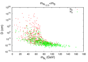
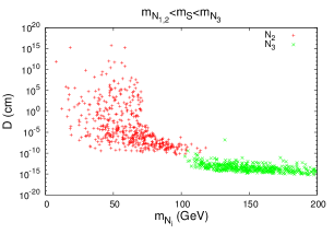
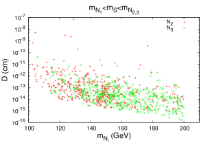
Figure 1: The distance $D_{i}$ travelled by the heavier RHNs as a function of their masses for the three cases: $m_{N_{1,2,3}}<m_{S}$ (left), $m_{N_{1,2}}<m_{S}<m_{N_{3}}$ (middle) and $m_{N_{1}}<m_{S}<m_{N_{2,3}}$ (right). Here, we consider the typical energy for $N_{2,3}$ to be $200\,GeV$.

It is clear from Fig. 1 that $N_{3}$ decays mostly inside the detector except for a few benchmark points in the case in which the charged scalar is the heaviest. For the RHN $N_{2}$, it decays inside the detector in the case in which it is heavier than the charged scalar. In the inverse case, it could decay either inside or outside the detector depending on the couplings.

A search with a negative result had been performed by the L3 Collaboration at LEP-II about a single photon with a missing energy signal at c.m. energies 189 and $209~{}\mathrm{GeV}$ with the corresponding luminosity values 176 and $130.2~{}\mathrm{pb^{-1}}$, respectively Achard:2003tx . Based on this negative search, we will constrain our parameters space.

Using LANHEP Semenov:2008jy to implement the model (6) and CALCHEP Belyaev:2012qa to compute the cross sections for the background $e^{-}e^{+}\rightarrow\nu\bar{\nu}\gamma$ and the signal $e^{-}e^{+}\rightarrow\gamma+\not{E}_{T}$, taking into account the same cuts used by LEP-II to search for the single photon events Achard:2003tx , we have the following:

$\bullet$ The polar angle of the photon is $|cos\theta^{\gamma}|<0.97$.

$\bullet$ The transverse momentum of photon must satisfy $p_{T}^{\gamma}>0.02~{}E_{c.m.}~{}(\mathrm{GeV})$.

$\bullet$ The energy of the photon must satisfy $E^{\gamma}>1~{}\mathrm{GeV}$.

At the end, we generate 3000 benchmark points that are in agreement with the bounds from the muon anomalous magnetic moment and the LFV processes $\ell_{\alpha}\rightarrow\ell_{\beta}+\gamma$ and $\ell_{\alpha}\rightarrow\ell_{\beta}+\bar{\ell_{\beta}}+\ell_{\beta}$. We distinguish two cases with $m_{N_{i}}=\{25,30,35~{}\mathrm{GeV}\}$ and $m_{N_{i}}=\{50,60,70~{}\mathrm{GeV}\}$. In Fig. 2, we display the significance of the signal $e^{-}e^{+}\rightarrow\gamma+\not{E}_{T}$ (in the palette) for different values of the coupling $\left|g_{1e}\right|$ and the charged scalar mass for the two cases mentioned previously.

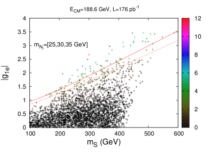
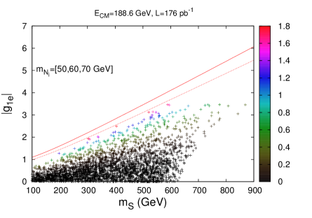
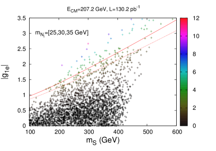
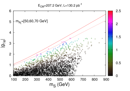
Figure 2: The coupling $\left|g_{1e}\right|$ as a function of $m_{S}$ for 3000 benchmark points with the two cases $m_{N_{i}}=\{25,30,35~{}\mathrm{GeV}\}$ (left) and $m_{N_{i}}=\{50,60,70~{}\mathrm{GeV}\}$ (right). The palette represents the signal significance $S$ of the process $e^{-}e^{+}\rightarrow\gamma+\not{E}_{T}$ for the c.m. energy values $E_{c.m.}=188.6$ (up) and $E_{c.m.}=207.2$ (down) with the integrated luminosity $L=176~{}pb^{-1}$ and $L=130.2~{}pb^{-1}$, respectively. The solid (dashed) line corresponds to the new constraint at LEP II, which makes the signal significance smaller than $\mathcal{S}<3$ $(\mathcal{S}<2)$. For most of the benchmark points used here, the missing energy is identified as $\not{E}_{T}=N_{1}N_{1}$, which justifies the choice of $\left|g_{1e}\right|$ in the y axes.

From Fig. 2, one can remark that once the LFV bounds are fulfilled the bound from LEP-II is also satisfied for $N_{1}$ heavier than $50~{}\mathrm{GeV}$, whereas LEP-II could exclude some benchmark points, especially using the analysis with $E_{c.m.}=207.2$ $\mathrm{GeV}$. For our analysis, we consider the following numerical values shown in Table 3, which we call model 3 ($M_{3}$) and model 4 ($M_{4}$). These values respect the muon anomalous magnetic moment and LFV bounds in Table 2.

Models Parameters $m_{N_{i}}\left(\mathrm{GeV}\right)$ $25.788,~{}28.885,~{}36.274$, $M_{3}$ $m_{S}$ $\left(\mathrm{GeV}\right)$ $196.75$, $g_{i\alpha}/10^{-2}$ $\left(\begin{array}[]{ccc}75.063-i0.14367&0.0026819-i0.015758&-136.03i-70.675\\ -3.6203-i35.9460&-0.0035368+i0.041316&120.47-i286.100\\ -3.0602-i0.49553&0.057628-i0.2462700&-235.27+i33.529\end{array}\right)$, $m_{N_{i}}\left(\mathrm{GeV}\right)$ $62.184,~{}76.275,~{}95.736$, $M_{4}$ $m_{S}$ $\left(\mathrm{GeV}\right)$ $126.78$, $g_{i\alpha}/10^{-2}$ $\left(\begin{array}[]{ccc}-60.008+i2.4015&-0.55187-i1.1133&-32.641+i41.313\\ 5.0213+i22.533&3.5209-i2.2480&-112.35-i32.473\\ 4.2829+i3.7764&-2.2562+i2.3886&-171.25-i94.890\end{array}\right)$.

Table 3: The parameters values for model 3 and model 4.

In Fig. 3, the normalized distribution of the travelled distance $D_{i}$ for the heavier RHNs $N_{2,3}$ is shown for $M_{3,4}$.

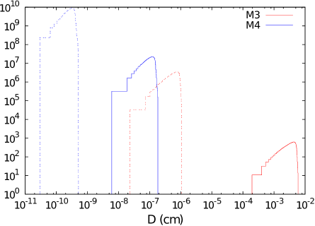
Figure 3: The normalized distribution of the travelled distance $D_{i}$ (in cm) by the heavier RHNs $N_{2}$ (solid) and $N_{3}$ (dashed) at $E_{c.m.}=500~{}\mathrm{GeV}$.

It is very clear that the travelled distance $D_{i}$ is very small for both heavy RHNs $N_{2,3}$ since their decay via a three-body process $N_{2,3}\rightarrow N_{1}+\ell_{\alpha}+\ell_{\beta}$ for both $M_{3}$ and $M_{4}$. This means that they both decay inside the detector and can be accounted for missing energy, i.e., $\not{E}_{T}=N_{1}N_{1}$.

III FINAL STATE $b\bar{b}+\not{E}_{T}$ AT $e^{-}e^{+}$ COLLIDERS

The $m_{h}=125.09~{}\mathrm{GeV}$ Higgs has the dominant decay mode ${\cal B}\left(h\rightarrow b\bar{b}\right)=57.7\%$ Olive:2016xmw , while the Z branching ratio ${\cal B}\left(Z\rightarrow b\bar{b}\right)=15.12\%$ Olive:2016xmw is also significant. Then, the choice of the channel $b\bar{b}+\not{E}_{T}$ is interesting since the b-tagging efficiency is shown to be about $80\%$ when the misidentification efficiencies for c jet and u/d/s jet are below $10\%$ and $1\%$, respectively, at both the ILC and CLIC Suehara:2015ura . This is encouraging in considering the $b\bar{b}$ final state for our studied models $M_{i}$ due to a possible clear signal. In this work, we want to probe the interactions (1) and (6) through the final state $b\bar{b}+\not{E}_{T}$ at a leptonic collider. This signal [Figs. 4(d) and  4(e)] has the background contributions $e^{-}e^{+}\rightarrow Z(Z,h,\gamma^{*})\rightarrow b\bar{b}+\not{E}_{T}$ [Fig. 4(a) and (b)] in addition to the W-fusion diagrams [Fig. 4(c)].

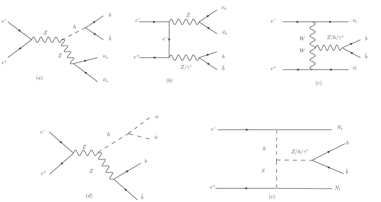
Figure 4: The most important Feynman diagrams that contribute to background (a), (b), and (c) [(d) and (e)] [the signal] for the process $e^{-}e^{+}\rightarrow b\bar{b}+\not{E}_{T}$.

Future experiments such as the ILC ILC4 ; Adolphsen:2013kya and CILC Battaglia:2004mw ; CLICP2 may use polarized beams of electrons and positrons. This feature could help us to identify the DM nature whether it is fermionic, vectorial, or scalar. Here, we will consider both cases with and without polarized beams. By varying the c.m. energy in the range $250~{}\mathrm{GeV}<E_{c.m.}<1~{}\mathrm{TeV}$, we get in Fig. 5 the cross section of different models and the background as a function of $E_{c.m.}$ with and without polarized beams.

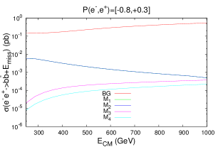
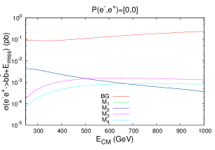
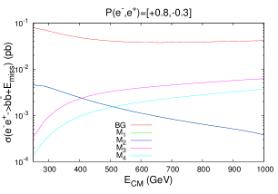
Figure 5: The cross section of different models and background as a function of $E_{c.m.}$ with the polarization $P\left(e^{-},e^{+}\right)=[-0.8,+0.3]$ (left) and $P\left(e^{-},e^{+}\right)=[+0.8,-0.3]$ (right) and without polarization (middle). These figures are produced using the packages LANHEP/CALCHEP Semenov:2008jy ; Belyaev:2012qa .

One can see from Fig. 5 that the cross sections of $M_{1}$ and $M_{2}$ are identical for the cases with polarized and unpolarized beams. This feature is a numerical accident since the cross section is proportional to the Higgs invisible branching ratio ${\cal B}_{inv}\left(h\rightarrow\phi\phi\right)$, which has the same numerical value for $M_{1}$ and $M_{2}$, so the aim of the choice in Table 1 is to find out the effect of the scalar mass $m_{\phi}$ and the coupling $c_{s}$. One notices also that the background cross section is increasing (decreasing) for the cases with the polarizations $P\left(e^{-},e^{+}\right)=[0,0]$ and $[-0.8,+0.3]$ ($P\left(e^{-},e^{+}\right)=[+0.8,-0.3]$) as a function of the c.m. energy. This guides us to not consider the polarization $P\left(e^{-},e^{+}\right)=[-0.8,+0.3]$ in our analysis. For $M_{3}$ and $M_{4}$, the cross section is increasing with respect $E_{c.m.}$ especially within the polarization $P\left(e^{-},e^{+}\right)=[+0.8,-0.3]$. Then, we will consider the c.m. energy values $E_{c.m.}=500~{}\mathrm{GeV}$ and $1~{}\mathrm{TeV}$ in the rest of our work.

The general signal significance definition is given by Cowan:2010js

$$\mathcal{S}=\sqrt{2\times\left[(N_{S}+N_{BG})\times log(1+N_{S}/N_{BG})-N_{S}\right]},$$ (8)

where $N_{S}$ and $N_{B}$ are the signal and background events numbers, respectively. Here, $N_{S}$ is given by

$$N_{S,BG}=\epsilon_{b}^{2}\times\mathcal{L}_{int}\times\sigma_{S,BG},$$ (9)

with $\epsilon_{b}=0.8$ being the b-tagging efficiency factor, $\mathcal{L}_{int}$ being the integrated luminosity, and $\sigma_{S,BG}$ being the signal or background cross section value.

IV Analysis and Discussion

In this work, we used LANHEP packages Semenov:2008jy to implement the models and generate their Feynman rules, and then we used CALCHep Belyaev:2012qa to estimate the cross section and produce the differential cross section for the background and signal at both $E_{c.m.}=500~{}\mathrm{GeV}$ and $1~{}\mathrm{TeV}$. To define the cuts on the kinematic variables that maximize the significance, we produced different distributions and looked for ranges in which the background is reduced while keeping the signal value. Therefore, we generated different distributions, taking into account the following pre-cuts:

$\bullet$ The transverse momentum of the bottom quark $\left(b\right)$ and the bottom antiquark $\left(\bar{b}\right)$ must satisfy $p_{T}>15$ $\ \mathrm{GeV}$.

$\bullet$ The missing energy $\not{E}_{T}>30\ \mathrm{GeV}$.

$\bullet$ The invariant mass of the bottom quark $\left(b\right)$ and the bottom antiquark $\left(\bar{b}\right)$ must be in the range $71~{}\mathrm{GeV}<M^{b,\bar{b}}<145~{}\mathrm{GeV}$.

$\bullet$ The jet separation radius must satisfy $\triangle R_{b,\bar{b}}>0.4$, where $\triangle R$ is given by

$$\triangle R=\sqrt{\triangle\phi^{2}+\triangle\eta^{2}},$$ (10)

where $\phi$ is the azimuthal angle and $\eta$ is the pseudorapidity.

The first two cuts helped too much to reduce the contamination in the signal region. To ensure that the $b\bar{b}$ pair was produced through a $Z$-gauge boson and/or the Higgs as shown in Figs. 4(d) and  4 (e), we considered the third cut.

In the first step, we considered unpolarized beams of electrons and positrons to generate the differential cross section for the background (SM) and the signal (the models $M_{i}$) at both c.m. energies $E_{c.m.}=500~{}\mathrm{GeV}$ and $1~{}\mathrm{TeV}$. Then, we looked for kinematical variables regions where the background was reduced and the signal was as maintained as possible. Then, the full set of cuts is given in Table 4.

$E_{c.m.}$ Selection cuts $500$ $15~{}<p_{T}^{b}~{}$,$~{}30~{}<\not{E}_{T}~{}$,$~{}71~{}<M^{b,\bar{b}}<145~{}$,$~{}0.4<\triangle R_{b,\bar{b}},~{}90~{}\leq E_{T}^{b,\bar{b}}\leq 230~{},~{}210~{}\leq M_{T}^{b,\not{E}_{T}},$ $1000$ $15~{}<p_{T}^{b}~{}$,$~{}30~{}<\not{E}_{T}~{}$,$~{}71~{}<M^{b,\bar{b}}<145~{}$,$~{}0.4<\triangle R_{b,\bar{b}}$,$125~{}\leq E_{T}^{b,\bar{b}}~{},~{}240~{}\leq M_{T}^{b,\not{E}_{T}}$.

Table 4: The full set of cuts for the process $e^{-}e^{+}\rightarrow b\bar{b}+\not{E}_{T}$ at both c.m. energies $E_{c.m.}=500~{}\mathrm{GeV}$ and $1~{}\mathrm{TeV}$. Here, $p_{T}^{b}$ is the transverse momentum of the bottom quark $\left(b\right)$, $\not{E}_{T}$ is the missing energy, $M^{b,\bar{b}}$ is the invariant mass of the bottom quark $\left(b\right)$ and the bottom antiquark $\left(\bar{b}\right)$, $\triangle R_{b,\bar{b}}$ is the jet cone angle, $E_{T}^{b,\bar{b}}$ is the transverse energy for the bottom quark $\left(b\right)$ and bottom antiquark $\left(\bar{b}\right)$, and $M_{T}^{b,\not{E}_{T}}$ is the transverse mass of bottom-missing energy. All masses and energies are given in $\mathrm{GeV}$.

IV.1 Analysis using unpolarized beams

By imposing the full set of cuts in Table 4 at both c.m. energies $E_{c.m.}=500~{}\mathrm{GeV}$, and $1~{}\mathrm{TeV}$, using unpolarized beams, we get the results shown in Table 5.

$E_{c.m.}~{}(\mathrm{GeV})$ $\sigma^{BG}~{}(fb)$ Models $\sigma^{S}~{}(fb)$ $\sigma^{\prime BG}~{}(fb)$ $\sigma^{\prime S}~{}(fb)$ $\mathcal{S}_{100}$ $\mathcal{S}_{500}$ $M_{1}$ $1.475$ $0.520$ $0.9808$ $2.1936$ $500$ $108.19$ $M_{2}$ $1.479$ $17.804$ $0.638$ $1.2024$ $2.6888$ $M_{3}$ $1.425$ $0.956$ $1.7960$ $4.0168$ $M_{4}$ $1.338$ $1.070$ $2.0088$ $4.4912$ $M_{1}$ $0.352$ $0.282$ $0.3216$ $0.7192$ $M_{2}$ $0.353$ $0.292$ $0.3328$ $0.7448$ $1000$ $233.27$ $M_{3}$ $1.265$ $49.072$ $0.942$ $1.0720$ $2.3976$ $M_{4}$ $0.954$ $0.760$ $0.8656$ $1.9352$

Table 5: The cross section values of the background and the signal for each model within the pre-cuts $\sigma^{BG}$, $\sigma^{S}$ and after applying the full cuts set given in Table 4 $\sigma^{\prime S}$,$\sigma^{\prime BG}$ at both c.m. energies $E_{c.m.}=500~{}\mathrm{GeV}$ and $1~{}\mathrm{TeV}$. The corresponding signal significance is shown for the luminosity values $L=100~{},~{}500~{}fb^{-1}$.

Through the results presented in Table 5, one notices that the signal cross section within the full set of cuts gets reduced a bit with respect to the case within the pre-cuts for all models at both $E_{c.m.}=500~{}\mathrm{GeV}$ and $1~{}\mathrm{TeV}$, whereas, the background cross section gets reduced by about $83.5\%$ ($79\%$) at $E_{c.m.}=500~{}\mathrm{GeV}$ ($E_{c.m.}=~{}1~{}\mathrm{TeV}$). For luminosity $L=100~{}fb^{-1}$, we do not see any deviation from the SM at both $E_{c.m.}=500~{}\mathrm{GeV}$ and $1~{}\mathrm{TeV}$. However, for $L=500~{}fb^{-1}$, one could notice a deviation from the SM at $E_{c.m.}=500~{}\mathrm{GeV}$ for $M_{3,4}$. At $E_{c.m.}=1~{}\mathrm{TeV}$, within the same luminosity value, we could not even see a deviation from the SM for all models. Therefore, for this c.m. energy, we require a large luminosity value (1 $ab^{-1}$ or more) in order to see such a signal.

In case of large luminosity values that allow the signal to be seen, we show relevant normalized distributions in Figs. 6 and  7, for $E_{c.m.}=500~{}\mathrm{GeV}$ and $1~{}\mathrm{TeV}$, respectively. The relevant distributions here are the polar angle between bottom-antibottom jets $cos(\theta^{b,\bar{b}})$, the jet energy $E^{b}$, the jet transverse energy $E_{T}^{b}=\sqrt{m_{b}^{2}+\overrightarrow{p}_{T}^{2}}$, the jet transverse momentum $p_{T}^{b}$, the transverse mass of the bottom-antibottom jets $M_{T}^{b,\bar{b}}=\sqrt{\left(E_{T}^{b}+E_{T}^{\bar{b}}\right)^{2}-\left(\overrightarrow{p}_{T}^{b}+\overrightarrow{p}_{T}^{\bar{b}}\right)^{2}}$, the invariant mass of the missing energy with a jet $M^{b,\not{E}_{T}}$, the jet pseudorapidity $\eta^{b}$, the two-jet pseudo rapidity $\eta^{b,\bar{b}}$, and the polar angle between the two jets in the boost direction $cos(\Theta^{b,\bar{b}})$.

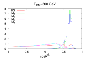
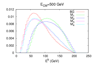
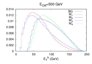
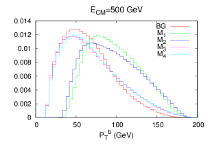
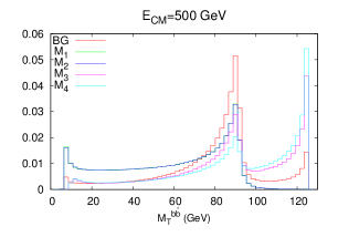
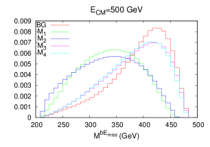
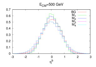
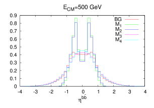
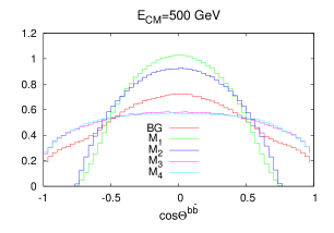
Figure 6: The relevant normalized distributions of the process $e^{-}e^{+}\rightarrow b\bar{b}+\not{E}_{T}$ at $E_{c.m.}=500~{}\mathrm{GeV}$.

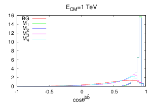
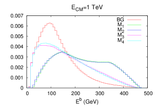
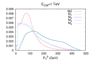
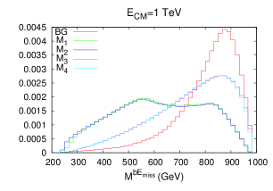
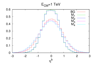
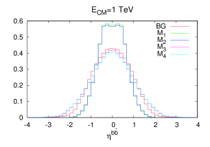
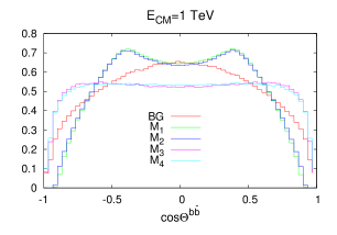
Figure 7: The relevant normalized distributions of the process $e^{-}e^{+}\rightarrow b\bar{b}+\not{E}_{T}$ at $E_{c.m.}=1~{}\mathrm{TeV}$.

At $E_{c.m.}=500~{}\mathrm{GeV}$ (Fig. 6), for scalar DM ($M_{1,2}$), the normalized distributions have different shapes with respect to both the background and the fermionic DM case ($M_{3,4}$), especially for the distributions $cos(\theta^{b,\bar{b}})$, $E^{b}$, $E_{T}^{b}$, $p_{T}^{b}$, $M^{b,\not{E}_{T}}$, $\eta^{b,\bar{b}}$, and $cos(\Theta^{b,\bar{b}})$. For the fermionic DM case ($M_{3,4}$), the normalized distributions have the same shape with respect to the background with a remarkable shift. For instance, if the DM is a scalar, the normalized distributions of $cos(\theta^{b,\bar{b}})$ and $\eta^{b,\bar{b}}$ get maximized for $0.4<cos(\theta^{b,\bar{b}})<0.8$ and $0.3<|\eta^{b,\bar{b}}|<0.8$, respectively. However, at $E_{c.m.}=1~{}\mathrm{TeV}$ (Fig. 7), the two cases of scalar and fermionic DM could be easily distinguished due to the different normalized distributions shapes.

IV.2 Analysis using polarized beams

In search of new physics, the use of polarized beams at future electron/positron colliders such as the ILC and CLIC could reduce the background and/or enhance the signal ILC4 ; Adolphsen:2013kya ; Baer:2013c.m.a . The electron or positron polarization is defined as

$$P\left(f\right)=(N_{f_{R}}-N_{f_{L}})/(N_{f_{R}}+N_{f_{L}}),$$ (11)

where $N_{f_{R}}$ ($N_{f_{L}}$) is the number of right- (left-) handed fermions. At the ILC, the polarization degree of the electron (positron) beams could reach $80\%$ ($30\%$), i.e., $|P(e^{-})|<0.80$ ($|P(e^{+})|)<0.30$) Adolphsen:2013kya . The positron polarization could be improved up to $60\%$ at the CLIC Battaglia:2004mw ; CLICP2 .

Here, we reanalyze the same process at the same c.m. energy values within the polarization $P\left(e^{-},e^{+}\right)=[+0.8,-0.3]$, while keeping the same full set of cuts given in Table 4. We present the results compared to the case without polarization in Table 6.

$P\left(e^{-},e^{+}\right)$ $=$ $[0,0]$ $P\left(e^{-},e^{+}\right)$ $=$ $[+0.8,-0.3]$ $E_{c.m.}$ $\left(\mathrm{GeV}\right)$ $\sigma^{BG}$$\left(fb\right)$ Models $\sigma^{S}$ $\left(fb\right)$ $\mathcal{S}_{100}$ $\mathcal{S}_{500}$ $\sigma^{BG}$ $\left(fb\right)$ $\sigma^{S}$ $\left(fb\right)$ $\mathcal{S}_{100}$ $\mathcal{S}_{500}$ $M1$ $0.520$ $0.9808$ $2.1936$ $0.558$ $1.9488$ $4.3584$ $500$ $17.804$ $M_{2}$ $0.638$ $1.2024$ $2.6888$ $5.061$ $0.685$ $2.3832$ $5.3304$ $M_{3}$ $0.956$ $1.7960$ $4.0168$ $2.166$ $7.2328$ $16.1736$ $M_{4}$ $1.070$ $2.0088$ $4.4912$ $2.570$ $8.4944$ $18.9944$ $M_{1}$ $0.282$ $0.3216$ $0.7192$ $0.303$ $0.7640$ $1.7096$ $M_{2}$ $0.292$ $0.3328$ $0.7448$ $0.313$ $0.7896$ $1.7656$ $1000$ $49.072$ $M_{3}$ $0.942$ $1.0720$ $2.3976$ $9.950$ $5.472$ $12.8312$ $28.6912$ $M_{4}$ $0.760$ $0.8656$ $1.9352$ $4.219$ $10.0520$ $22.4784$

Table 6: The cross section values for the background $\sigma^{BG}$ and the signal $\sigma^{S}$ estimated for the considered energies within the full set of cuts given in Table 4, without and with polarized beams at both c.m. energies $E_{c.m.}=500~{}\mathrm{GeV}$ and $1~{}\mathrm{TeV}$. The significances $\mathcal{S}_{100}$ and $\mathcal{S}_{500}$ correspond to the two integrated luminosity values $L=100~{}fb^{-1}$ and $500~{}fb^{-1}$, respectively.

From Table 6, by comparing the cases with and without polarization, one remarks that the cross section value for the background $\sigma^{BG}$ is reduced by about $72\%$ ($80\%$) at $E_{c.m.}=500~{}\mathrm{GeV}$ ($E_{c.m.}=1~{}\mathrm{TeV}$). On the contrary, the signal cross section value $\sigma^{S}$ gets increased by about $7\%$ for both $M_{1,2}$ at both c.m. energies $E_{c.m.}=500~{}\mathrm{GeV}$ and $1~{}\mathrm{TeV}$. One can also see the cross section value for $M_{3}$ ($M_{4}$) gets raised by about $127\%$ ($140\%$) and by $481\%$ ($455\%$) for c.m. energies $500~{}\mathrm{GeV}$ and $~{}1~{}\mathrm{TeV}$ respectively. Consequently, the signal significance gets enhanced by $303\%$ ($323\%$) and by $1097\%$ ($1061\%$) for $M_{3}$ ($M_{4}$) at $500~{}\mathrm{GeV}$ and $~{}1~{}\mathrm{TeV}$, respectively. When considering the polarization $P\left(e^{-},e^{+}\right)=[+0.8,-0.3]$, the background cross section gets decreased sharply due to the vertices suppression of the electron-positron with gauge bosons unlike the vertices of the charged scalar-Majorana fermion-charged lepton (for $M_{3,4}$), which enhances the cross section.

For luminosity $L=100~{}fb^{-1}$, one discovers for $M_{3,4}$ at both $E_{c.m.}=500~{}\mathrm{GeV}$ and $1~{}\mathrm{TeV}$; however, for $L=500~{}fb^{-1}$, one can see also a discovery for all models at $E_{c.m.}=500~{}\mathrm{GeV}$ except Model 1. At $E_{c.m.}=1~{}\mathrm{TeV}$ within the same luminosity, we could not even see a deviation from the SM for $M_{1,2}$, unlike $M_{3,4}$ in which one can clearly see a discovery. Therefore, we require a large luminosity value (1 $ab^{-1}$ or more) in order to see such a signal for two models $M_{1,2}$ in which DM is a scalar.

In Figs. 8 and  9, we show the relevant normalized distributions at $E_{c.m.}=500~{}\mathrm{GeV}$ and $1~{}\mathrm{TeV}$, respectively, using the polarized beams $P\left(e^{-},e^{+}\right)=[+0.8,-0.3]$.

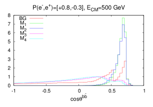
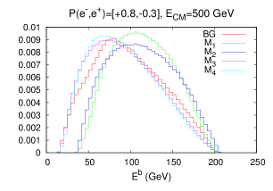
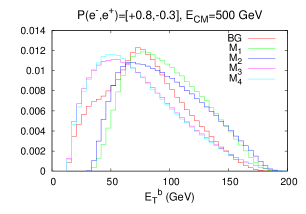
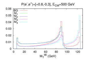
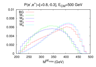
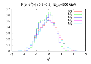
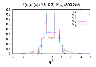
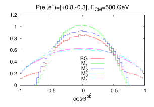
Figure 8: The relevant normalized distributions of the process $e^{-}e^{+}\rightarrow b\bar{b}+\not{E}_{T}$ at $E_{c.m.}=500~{}\mathrm{GeV}$ with polarized beams $P\left(e^{-},e^{+}\right)=[+0.8,-0.3]$.

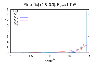
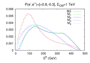
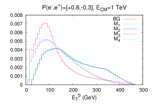
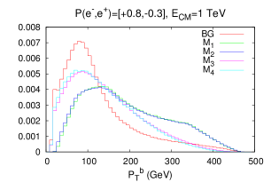
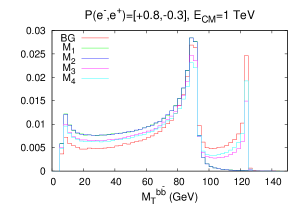
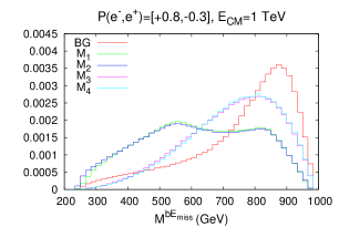
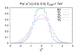
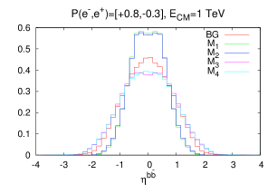
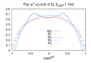
Figure 9: The relevant normalized distributions of the process $e^{-}e^{+}\rightarrow b\bar{b}+\not{E}_{T}$ at $E_{c.m.}=1~{}\mathrm{TeV}$ with polarized beams $P\left(e^{-},e^{+}\right)=[+0.8,-0.3]$.

From Fig. 8, for scalar DM ($M_{1,2}$), the normalized distributions have different shapes with respect to the background, especially for the distributions: $E_{T}^{b}$, $p_{T}^{b}$, $M^{b,\not{E}_{T}}$, $\eta^{b}$, and $cos(\Theta^{b,\bar{b}})$. However, for fermionic DM ($M_{3,4}$), the distributions shape is different for $cos(\theta^{b,\bar{b}}),$$E^{b}$,$E_{T}^{b}$, $p_{T}^{b}$, $M^{b,\not{E}_{T}}$, $\eta^{b,\bar{b}}$, and $cos(\Theta^{b,\bar{b}})$. From Fig. 9, one notices that the normalized distributions $E^{b}$, $E_{T}^{b}$, $p_{T}^{b}$, $M^{b,\not{E}_{T}}$, and $cos(\Theta^{b,\bar{b}})$ have different shapes between the background, the scalar DM ($M_{1,2}$), and the fermionic DM cases ($M_{3,4}$). One remarks also that for the background and the fermionic DM case ($M_{3,4}$) the normalized distributions have the same shape especially for $cos(\theta^{b,\bar{b}}),~{}\eta^{b}$, and $\eta^{b,\bar{b}}$.

By comparing the results produced at $E_{c.m.}=500~{}\mathrm{GeV}$ using polarized beams (Fig. 8) with those without polarization (Fig. 6), one can notice a clear difference. For instance, if the DM is a scalar, the maximum of the normalized distributions of $E^{b}$, $p_{T}^{b}$, and $\eta^{b}$ get shifted into $30~{}\mathrm{GeV}<E^{b}<70~{}\mathrm{GeV}$, $15~{}\mathrm{GeV}<p_{T}^{b}<65~{}\mathrm{GeV}$, and $-1<\eta^{b}<0.2$, respectively, with respect to the case without polarization. At $E_{c.m.}=1~{}\mathrm{TeV}$, for the fermionic DM case ($M_{3,4}$), the maximum of the normalized distributions of $M^{b,\not{E}_{T}}$ and $cos(\Theta^{b,\bar{b}})$ get shifted also into $450~{}\mathrm{GeV}<M^{b,\not{E}_{T}}<780~{}\mathrm{GeV}$ and $|cos(\Theta^{b,\bar{b}})|<0.4$, respectively.

To get idea about the required values for the luminosity to observe such a deviation or a discovery, we estimate the signal significance by varying integrated luminosity values $L$. We show in Fig. 10 the signal significance for different models, using polarized and unpolarized beams

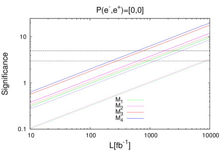
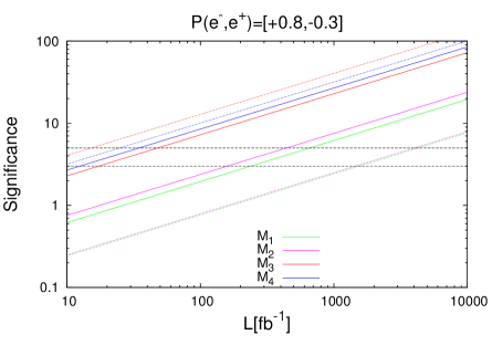
Figure 10: The significance $\mathcal{S}$ vs luminosity $L$ at different c.m. energies (solid lines at $500~{}\mathrm{GeV}$, the dashed lines at $1~{}\mathrm{TeV}$) within the full set of cuts given in Table 4, without (left) and with (right) polarized beam. The two horizontal dashed lines represent $\mathcal{S}=3$ and $\mathcal{S}=5$, respectively.

From Fig. 10, one remarks easily that the use of polarized beams (with the polarization $P\left(e^{-},e^{+}\right)=[+0.8,-0.3]$) makes the signal detected with smaller integrated luminosity as compared to the case with unpolarized beams for each model and at $E_{c.m.}=500~{}\mathrm{GeV}$,$~{}1~{}\mathrm{TeV}$. For example, at $E_{c.m.}=500~{}\mathrm{GeV}$, a $5\sigma$ significance requires a minimal luminosity value $750~{}\mathrm{fb^{-1}}$ ($600~{}\mathrm{fb^{-1}}$ ) for $M_{3}$ ($M_{4}$) using unpolarized beams. Using polarized beams, this minimal luminosity value becomes $45~{}\mathrm{fb^{-1}}$ ($30~{}\mathrm{fb^{-1}}$) for $M_{3}$ ($M_{4}$). Similar remarks hold for the models $M_{1,2}$, where the required luminosity gets decreased form 2500 (1700) to $650~{}\mathrm{fb^{-1}}$ ($430~{}\mathrm{fb^{-1}}$) for $M_{1}$ ($M_{2}$).

In Table 7, we summarize the events number for the background and the signal for the different models using polarized and unpolarized beams at $E_{c.m.}=500~{}\mathrm{GeV}$ and $1~{}\mathrm{TeV}$.

$P\left(e^{-},e^{+}\right)$ $=$ $[0,0]$ $P\left(e^{-},e^{+}\right)$ $=$ $[+0.8,-0.3]$ $E_{c.m.}~{}(\mathrm{GeV})$ $N_{BG}$ Models $N_{S}$ $\mathcal{S}_{100}$ $\mathcal{S}_{500}$ $N_{BG}$ $N_{S}$ $\mathcal{S}_{100}$ $\mathcal{S}_{500}$ $M1$ $33.2864$ $0.9808$ $2.1936$ $35.7120$ $1.9488$ $4.3584$ $500$ $1139.456$ $M_{2}$ $40.8320$ $1.2024$ $2.6888$ $323.904$ $43.8400$ $2.3832$ $5.3304$ $M_{3}$ $61.1840$ $1.7960$ $4.0168$ $138.6368$ $7.2328$ $16.1736$ $M_{4}$ $68.4800$ $2.0088$ $4.4912$ $164.4864$ $8.4944$ $18.9944$ $M_{1}$ $18.0608$ $0.3216$ $0.7192$ $19.4048$ $0.7648$ $1.7104$ $M_{2}$ $18.6944$ $0.3328$ $0.7448$ $20.0320$ $0.7896$ $1.7656$ $1000$ $3140.608$ $M_{3}$ $60.2880$ $1.0720$ $2.3976$ $636.8064$ $350.2080$ $12.8312$ $28.6912$ $M_{4}$ $48.6528$ $0.8656$ $1.9360$ $270.0224$ $10.0528$ $22.4784$

Table 7: The background and signal events number $N_{BG}$, $N_{S}$ estimated for the considered energies within the full set of cuts given in Table 4, without and with polarized beams at both c.m. energies $E_{c.m.}=500~{}\mathrm{GeV}$ and $1~{}\mathrm{TeV}$. The significance $\mathcal{S}_{100}$ and $\mathcal{S}_{500}$ correspond to the two integrated luminosity values $L=100$ and $500~{}fb^{-1}$, respectively.

The results presented in Table 7 give evidence that with the polarization $P\left(e^{-},e^{+}\right)=[+0.8,-0.3]$ suppresses the background $N_{BG}$ events number by $72\%$ and by $80\%$ for $E_{c.m.}=500~{}\mathrm{GeV}$ and $1~{}\mathrm{TeV}$, respectively. Simultaneously, the signal $N_{S}$ number of events for $M_{3}$ ($M_{4}$) gets improved by $127\%$ ($140\%$) and by $481\%$ ($455\%$) for c.m. energies $500~{}\mathrm{GeV}$ and $1~{}\mathrm{TeV}$, respectively. This (significant) excess of events numbers could be an indication of the nature of DM; i.e., if the DM is a heavy RHN, the excess could be about five times.

V Conclusions

In this work, we have investigated the possibility of detecting the signal significance of DM and identifying its nature. In our setup, the DM could be either a real scalar or heavy RHN produced at future electron-positron linear colliders such as the ILC and CLIC. To realize this task, we considered the process $e^{-}e^{+}\rightarrow b\bar{b}+\not{E}_{T}$ at two different c.m. energies: $E_{c.m.}=500~{}\mathrm{GeV}$ and $1~{}\mathrm{TeV}$. Here, we considered two parameter values sets for both scalar and RHN cases, four models, and we defined and investigated different experimental constraints for each case, such as the Higgs invisible decay, the muon anomalous magnetic moment, lepton flavor violation, DM relic density, and possible constraints from LEP-II. The latter constraint comes from the negative search of the monophoton at LEP-II, i.e., from the process $e^{-}e^{+}\rightarrow\gamma+\not{E}_{T}$, which is translated into bounds on the DM and charged scalar masses and the Yukawa coupling $|g_{1e}|$.

We found that when using appropriate cuts (in Table 4), the background gets significantly decreased and the signal significance gets lifted especially for the heavy RHN DM case. Using unpolarized beams at $E_{c.m.}=500~{}\mathrm{GeV}$, the DM nature can be distinguished using the normalized distributions: $E_{T}^{b}$, $p_{T}^{b}$, $M^{b,\not{E}_{T}}$, $\eta^{b,\bar{b}}$, and $cos(\Theta^{b,\bar{b}})$. However, a remarkable shift can be observed in most of the distributions for the fermioinc DM case. At $E_{c.m.}=1~{}TeV$, the DM nature can be also distinguished whether it is scalar or fermioinc using the different distributions.

Using polarized beams, the shape difference with respect to the background for most of the distributions is more clear, and smaller values of luminosity with respect of the case without polarized beams are required. Although, using the polarization $P\left(e^{-},e^{+}\right)=[+0.8,-0.3]$, the background cross section gets suppressed by about 80%, and/or the signal one gets enhanced. This leads to a significant enhancement on the statistical significance by double if the DM is a scalar and by five times if the DM is a heavy RHN.

Acknowledgements

This work is supported by the Algerian Ministry of Higher Education and Scientific Research under the CNEPRU Project No. B00L02UN180120140040. N. Baouche thanks the ICTP where part of this project was realized for the warm hospitality. We want to thank Junping Tian for his useful comments and clarifications. We would like to thank Salah Nasri, Luigi Delle Rose, and Rikard Enberg for reading the manuscript and for their useful comments.

References

- (1) G. Aad et al. [ATLAS Collaboration ], Phys. Lett. B 716, 1 (2012) [arXiv:1207.7214 [hep-ex]].
- (2) S. Chatrchyan et al. [c.m.S Collaboration], Phys. Lett. B 716, 30 (2012) [arXiv:1207.7235 [hep-ex]].
- (3) S. Fukuda et al. [Super-Kamiokande Collaboration], Phys. Rev. Lett. 86, 5651 (2001) [hep-ex/0103032]. Q. R. Ahmad et al. [SNO Collaboration], Phys. Rev. Lett. 87, 071301 (2001) [nucl-ex/0106015].
- (4) M. Gell-Mann, P. Ramond, and R. Slansky, in Supergravity, edited by P. van Nieuwenhuizen and D. Z. Freedman (North-Holland, Amsterdam, 1979), p. 315; T. Yanagida, in Proceedings of the Workshop on the Unified Theory and the Baryon Number in the Universe, edited by O. Sawada and A. Sugamoto, KEK Report No. 79-18 (Tsukuba, Japan, 1979), p. 95; R. N. Mohapatra and G. Senjanovic, Phys. Rev. Lett. 44, 912 (1980). J. Schechter and J. W. F. Valle, Phys. Rev. D 22, 2227 (1980). J. Schechter and J. W. F. Valle, Phys. Rev. D 25, 774 (1982).
- (5) T. P. Cheng and L. F. Li, Phys. Rev. D 22, 2860 (1980).
- (6) A. Zee, Phys. Lett. 93B, 389 (1980) Erratum: [Phys. Lett. 95B, 461 (1980)].
- (7) E. Ma, Phys. Rev. Lett. 81, 1171 (1998) [hep-ph/9805219].
- (8) A. Zee, Nucl. Phys. B 264, 99 (1986).
- (9) K. S. Babu, Phys. Lett. B 203, 132 (1988).
- (10) L. M. Krauss, S. Nasri and M. Trodden, Phys. Rev. D 67, 085002 (2003) [hep-ph/0210389].
- (11) M. Aoki, S. Kanemura and O. Seto, Phys. Rev. Lett. 102, 051805 (2009) [arXiv:0807.0361 [hep-ph]]; M. Aoki, S. Kanemura and O. Seto, Phys. Rev. D 80, 033007 (2009) [arXiv:0904.3829 [hep-ph]].
- (12) M. Gustafsson, J. M. No and M. A. Rivera, Phys. Rev. Lett. 110, no. 21, 211802 (2013) Erratum: [Phys. Rev. Lett. 112, no. 25, 259902 (2014)] [arXiv:1212.4806 [hep-ph]].
- (13) S. M. Boucenna, S. Morisi and J. W. F. Valle, Adv. High Energy Phys. 2014, 831598 (2014) [arXiv:1404.3751 [hep-ph]]; Y. Cai, J. Herrero-Garcia, M. A. Schmidt, A. Vicente and R. R. Volkas, arXiv:1706.08524 [hep-ph].
- (14) H. Okada and K. Yagyu, Phys. Rev. D 93, no. 1, 013004 (2016) [arXiv:1508.01046 [hep-ph]]; L. G. Jin, R. Tang and F. Zhang, Phys. Lett. B 741, 163 (2015) [arXiv:1501.02020 [hep-ph]]; K. Cheung, T. Nomura and H. Okada, arXiv:1610.04986 [hep-ph]; S. Baek, H. Okada and T. Toma, JCAP 1406, 027 (2014) [arXiv:1312.3761 [hep-ph]]; S. Kashiwase, H. Okada, Y. Orikasa and T. Toma, Int. J. Mod. Phys. A 31, no. 20n21, 1650121 (2016) [arXiv:1505.04665 [hep-ph]]; S. Kanemura, K. Nishiwaki, H. Okada, Y. Orikasa, S. C. Park and R. Watanabe, PTEP 2016, no. 12, 123B04 (2016) [arXiv:1512.09048 [hep-ph]]; S. Kanemura, O. Seto and T. Shimomura, Phys. Rev. D 84, 016004 (2011). E. Ma, Phys. Rev. D 73, 077301 (2006) [hep-ph/0601225]. A. Ahriche, C. S. Chen, K. L. McDonald and S. Nasri, Phys. Rev. D 90, 015024 (2014) [arXiv:1404.2696 [hep-ph]]. A. Ahriche, K. L. McDonald and S. Nasri, JHEP 1410, 167 (2014) [arXiv:1404.5917 [hep-ph]]. L. Megrelidze and Z. Tavartkiladze, Nucl. Phys. B 914, 553 (2017) [arXiv:1609.07344 [hep-ph]].
- (15) A. Ahriche, K. L. McDonald and S. Nasri, JHEP 1602, 038 (2016) [arXiv:1508.02607 [hep-ph]]. A. Ahriche, K. L. McDonald and S. Nasri, JHEP 1606, 182 (2016) [arXiv:1604.05569 [hep-ph]].
- (16) M. Aoki, S. Kanemura, K. Sakurai and H. Sugiyama, Phys. Lett. B 763, 352 (2016) [arXiv:1607.08548 [hep-ph]]. P. Fileviez Perez, T. Han, G. Y. Huang, T. Li and K. Wang, Phys. Rev. D 78, 071301 (2008) [arXiv:0803.3450 [hep-ph]]. C. S. Chen, C. Q. Geng, J. N. Ng and J. M. S. Wu, JHEP 0708, 022 (2007) [arXiv:0706.1964 [hep-ph]]. J. Kersten and A. Y. Smirnov, Phys. Rev. D 76, 073005 (2007) [arXiv:0705.3221 [hep-ph]]. A. Das and N. Okada, Phys. Rev. D 88, 113001 (2013) [arXiv:1207.3734 [hep-ph]]. D. Atwood, S. Bar-Shalom and A. Soni, Phys. Rev. D 76, 033004 (2007) [hep-ph/0701005]. S. Antusch, E. Cazzato and O. Fischer, JHEP 1604, 189 (2016) [arXiv:1512.06035 [hep-ph]]. S. Antusch, E. Cazzato and O. Fischer, Int. J. Mod. Phys. A 32 (2017) no.14, 1750078 [arXiv:1612.02728 [hep-ph]].
- (17) A. Ahriche, S. Nasri and R. Soualah, Phys. Rev. D 89, no. 9, 095010 (2014) [arXiv:1403.5694 [hep-ph]]. C. Guella, D. Cherigui, A. Ahriche, S. Nasri and R. Soualah, Phys. Rev. D 93, no. 9, 095022 (2016) [arXiv:1601.04342 [hep-ph]]. D. Cherigui, C. Guella, A. Ahriche and S. Nasri, Phys. Lett. B 762, 225 (2016) [arXiv:1605.03640 [hep-ph]].S. Y. Ho and J. Tandean, Phys. Rev. D 89, 114025 (2014) [arXiv:1312.0931 [hep-ph]]. S. Kanemura, T. Nabeshima and H. Sugiyama, Phys. Rev. D 87, no. 1, 015009 (2013) [arXiv:1207.7061 [hep-ph]].
- (18) M. Chekkal, A. Ahriche, A. B. Hammou and S. Nasri, Phys. Rev. D 95, no. 9, 095025 (2017) [arXiv:1702.04399 [hep-ph]].
- (19) M. Lindner, M. Platscher and F. S. Queiroz, arXiv:1610.06587 [hep-ph].
- (20) P. Achard et al. [L3 Collaboration ], Phys. Lett. B 587, 16 (2004) [hep-ex/0402002].
- (21) T. Behnke, C. Damerell, J. Jaros, A. Miyamoto et al. (ILC Collaboration), arXiv:0712.2356 [physics.ins-det].
- (22) C. Adolphsen et al., arXiv:1306.6328 [physics.acc-ph].
- (23) H. Baer et al., arXiv:1306.6352 [hep-ph].
- (24) M. J. Boland et al. [CLIC and CLICdp Collaborations], arXiv:1608.07537 [physics.acc-ph].
- (25) T. Suehara and T. Tanabe, Nucl. Instrum. Meth. A 808, 109 (2016) [arXiv:1506.08371 [physics.ins-det]].
- (26) C. Drig, K. Fujii, J. List and J. Tian, arXiv:1403.7734 [hep-ex].
- (27) Y. Mambrini, Phys. Rev. D 84, 115017 (2011) [arXiv:1108.0671 [hep-ph]]. X. G. He and J. Tandean, Phys. Rev. D 84, 075018 (2011) [arXiv:1109.1277 [hep-ph]]. G. Belanger, K. Kannike, A. Pukhov and M. Raidal, JCAP 1301, 022 (2013) [arXiv:1211.1014 [hep-ph]]. J. M. Cline, K. Kainulainen, P. Scott and C. Weniger, Phys. Rev. D 88, 055025 (2013) Erratum: [Phys. Rev. D 92, no. 3, 039906 (2015)] [arXiv:1306.4710 [hep-ph]]. H. Han, J. M. Yang, Y. Zhang and S. Zheng, Phys. Lett. B 756, 109 (2016) [arXiv:1601.06232 [hep-ph]]. A. Abada, D. Ghaffor and S. Nasri, Phys. Rev. D 83, 095021 (2011) [arXiv:1101.0365 [hep-ph]]. A. Abada and S. Nasri, Phys. Rev. D 85, 075009 (2012) [arXiv:1201.1413 [hep-ph]].
- (28) A. Ahriche and S. Nasri, Phys. Rev. D 85, 093007 (2012) [arXiv:1201.4614 [hep-ph]].
- (29) A. Birkedal, K. Matchev and M. Perelstein, Phys. Rev. D 70, 077701 (2004) [hep-ph/0403004].
- (30) C. Patrignani et al. [Particle Data Group], Chin. Phys. C 40, no. 10, 100001 (2016).
- (31) S. Heinemeyer et al. [LHC Higgs Cross Section Working Group], arXiv:1307.1347 [hep-ph].
- (32) A. Ahriche and S. Nasri, JCAP 1307, 035 (2013) [arXiv:1304.2055 [hep-ph]].
- (33) A. Ahriche, K. L. McDonald and S. Nasri, arXiv:1505.04320 [hep-ph].
- (34) T. Toma and A. Vicente, JHEP 1401, 160 (2014) [arXiv:1312.2840 [hep-ph]].
- (35) J. Hisano, T. Moroi, K. Tobe and M. Yamaguchi, Phys. Rev. D 53, 2442 (1996) [hep-ph/9510309].
- (36) C. W. Chiang, H. Okada and E. Senaha, Phys. Rev. D 96, no. 1, 015002 (2017) [arXiv:1703.09153 [hep-ph]]. D. A. Dicus, H. J. He and J. N. Ng, Phys. Rev. Lett. 87, 111803 (2001) [hep-ph/0103126]. T. Nomura, H. Okada and Y. Orikasa, Phys. Rev. D 94, no. 5, 055012 (2016) [arXiv:1605.02601 [hep-ph]]. T. Nomura and H. Okada, Phys. Rev. D 94, 075021 (2016) [arXiv:1607.04952 [hep-ph]]. K. S. Babu and J. Julio, Nucl. Phys. B 841, 130 (2010) [arXiv:1006.1092 [hep-ph]]. S. Lee, T. Nomura and H. Okada, arXiv:1702.03733 [hep-ph].
- (37) A. M. Baldini et al. [MEG Collaboration], Eur. Phys. J. C 76, no. 8, 434 (2016) [arXiv:1605.05081 [hep-ex]].
- (38) B. Aubert et al. [BaBar Collaboration ], Phys. Rev. Lett. 104, 021802 (2010) [arXiv:0908.2381 [hep-ex]].
- (39) K. Hayasaka et al., Phys. Lett. B 687, 139 (2010) [arXiv:1001.3221 [hep-ex]].
- (40) U. Bellgardt et al. [SINDRUM Collaboration], Nucl. Phys. B 299, 1 (1988).
- (41) P. A. R. Ade et al. [Planck Collaboration], Astron. Astrophys. 594, A13 (2016) [arXiv:1502.01589 [astro-ph.CO]].
- (42) A. Semenov, Comput. Phys. Commun. 180, 431 (2009) [arXiv:0805.0555 [hep-ph]].
- (43) A. Belyaev, N. D. Christensen and A. Pukhov, Comput. Phys. Commun. 184, 1729 (2013) [arXiv:1207.6082 [hep-ph]].
- (44) E. Accomando et al. [CLIC Physics Working Group], hep-ph/0412251.
- (45) R.W.Assmann and F. Zimmermann, SNOWMASS-2001-E3014, CERN-SL-2001-064-AP, CERN-CLIC-NOTE-501, CLIC-NOTE-501; W. Liu, W. Gai, L. Rinolfi,and J. Sheppard, Conf.Proc. C100523, THPEC035 (2010).
- (46) G. Cowan, K. Cranmer, E. Gross and O. Vitells, Eur. Phys. J. C 71, 1554 (2011) Erratum: [Eur. Phys. J. C 73, 2501 (2013)] [arXiv:1007.1727 [physics.data-an]].