Electronic structure of FeSe monolayer superconductors: shallow bands and correlations

Abstract

Electronic spectra of typical single FeSe layer superconductors – FeSe monolayer films on SrTiO₃ substrate (FeSe/STO) and K_xFe_2-ySe₂ obtained from ARPES data reveal several puzzles: what is the origin of shallow and the so called “replica” bands near M-point and why the hole-like Fermi surfaces near $\Gamma$-point are absent. Our extensive LDA+DMFT calculations show that correlation effects on Fe-3d states can almost quantitatively reproduce rather complicated band structure, which is observed in ARPES, in close vicinity of the Fermi level for FeSe/STO and K_xFe_2-ySe₂. Rather unusual shallow electron-like bands around the M(X)-point in the Brillouin zone are well reproduced. However, in FeSe/STO correlation effects are apparently insufficient to eliminate the hole-like Fermi surfaces around the $\Gamma$-point, which are not observed in most ARPES experiments. Detailed analysis of the theoretical and experimental quasiparticle bands with respect to their origin and orbital composition is performed. It is shown that for FeSe/STO system the LDA calculated Fe-3d_xy band, renormalized by electronic correlations within DMFT gives the quasiparticle band almost exactly in the energy region of the experimentally observed “replica” quasiparticle band at the M-point. For the case of K_xFe_2-ySe₂ most bands observed in ARPES can also be understood as correlation renormalized Fe-3d LDA calculated bands, with overall semi-quantitative agreement with our LDA+DMFT calculations. Thus the shallow bands near the M-point are common feature for FeSe-based systems, not just FeSe/STO. We also present some simple estimates of “forward scattering” electron-optical phonon interaction at FeSe/STO interface, showing that it is apparently irrelevant for the formation of “replica” band in this system and significant increase of superconducting $T_{c}$.

I Introduction

The discovery of a class of iron pnictide superconductors has revived the intensive search and studies of new of high-temperature superconductors (cf. reviews [Sadovskii, 2008; Ishida et al., 2009; Johnston, 2010; Hirschfeld et al., 2011; Stewart, 2011; Kordyuk, 2012]). Now there is general agreement that despite many similarities the nature of superconductivity in these materials significantly differs from that in high – $T_{c}$ cuprates, and further studies of these new systems may lead to better understanding of the problem of high-temperature superconductivity in general.

Actually, the discovery of superconductivity in iron pnictides was very soon followed by its discovery in iron chalcogenide FeSe, which attracted much interest due to its relative simplicity, though its superconducting characteristics (under normal conditions) were rather modest ($T_{c}\sim$8K). Its electronic structure is now well understood and quite similar to that of iron pnictides (cf. review in [Mizuguchi and Takano, 2010]).

However, the general situation with iron chalcogenides has changed rather dramatically with the appearance of intercalated FeSe based systems raising the value of $T_{c}$ to 30-40K. It was soon recognized that their electronic structure is in general rather different form that in iron pnictides [Sadovskii et al., 2012; Nekrasov and Sadovskii, 2014]. The first system of this kind was A_xFe_2-ySe₂ (A=K,Rb,Cs) with $T_{c}\sim$ 30K [Guo et al., 2010; Yan et al., 2012]. It is generally believed that superconductivity in this system appears in an ideal 122-type structure, though most of the samples studied so far were multiphase, consisting of a mixture of mesoscopic superconducting and insulating (antiferromagnetic) structures (e.g. such as K₂Fe₄Se₅), complicating the studies of this system [Krzton-Maziopa et al., 2016].

Further increase of $T_{c}$ up to 45K has been achieved by intercalation of FeSe layers with rather large molecules in compounds such as Li_x(C₂H₈N₂)Fe_2-ySe₂ [Hatakeda et al., 2013] and Li_x(NH₂)_y(NH₃)_1-yFe₂Se₂ [Burrard-Lucas et al., 2013]. The growth of $T_{c}$ in these systems is sometimes associated with increase of the distance between the FeSe layers, i.e. with the growth of the two-dimensional nature of the materials. Recently the active studies has started of [Li_1-xFe_xOH]FeSe system with the value of $T_{c}\sim$43K [Lu et al., 2014; Pachmayr et al., 2015], where a good enough single – phase samples and single crystals were obtained.

A significant breakthrough in the studies of iron chalcogenide superconductors occurred with the observation of a record high $T_{c}$ in epitaxial films of single FeSe monolayer on SrTiO₃(STO) substrate [Wang et al., 2012]. These films were grown in Ref. [Wang et al., 2012] and in most of the papers to follow on the 001 plane of the STO. It should be noted that these films are very unstable on the air. Thus in many works the resistive transitions were mainly studied on films covered with amorphous Si or several FeTe layers, which significantly reduced the observed values of $T_{c}$. Unique measurements of the resistance of FeSe films on STO, done in Ref. [Ge et al., 2014] in situ, produced the record values of $T_{c}>$100K. However, up to now these results were not confirmed by independent measurements. Many ARPES measurements of the temperature behavior of superconducting gap in such films, now confidently demonstrate the values of $T_{c}$ in the range of 65–75K, sometimes even higher.

Films consisting of several FeSe layers usually produce the values of $T_{c}$ much lower than those for the single – layer films [Miyata et al., 2015]. Monolayer FeSe film on 110 plane of STO covered with several FeTe layers was studied in Ref. [Zhou et al., 2016]. Resistivity measurements (including the measurements of the upper critical magnetic field $H_{c2}$) produced the value of $T_{c}\sim$30K. FeSe film, grown on BaTiO₃ (BTO) substrate, doped with Nb (with even larger values of the lattice constant $\sim$ 3.99 Å), showed (in ARPES measurements) the value of $T_{c}\sim$ 70K [Peng et al., 2014]. In Ref. [Ding et al., 2016] quite high values of the superconducting gap were reported (from tunneling spectroscopy) for FeSe monolayers grown on 001 plane of TiO₂ (anatase), which in its turn was grown on the 001 plane of SrTiO₃. The lattice constant of anatase is actually very close to the lattice constant of bulk FeSe, so these FeSe film were essentially unstretched.

Single – layer FeSe films were also grown on the graphene substrate, but the value of $T_{c}$ obtained was of the order of 8-10K as in bulk FeSe [Song et al., 2011]. This emphasizes the possible unique role of substrates such as Sr(Ba)TiO₃ in the significant increase of $T_{c}$.

More information on FeSe/STO films and other monolayer FeSe systems can be found in recent reviews [Krzton-Maziopa et al., 2016; Liu et al., 2015; Sadovskii, 2016].

II Crystal structures of iron based superconductors

In Figure 1 we schematically show the simple crystal structure of typical iron based superconductors [Mizuguchi and Takano, 2010; Sadovskii, 2008; Ishida et al., 2009; Johnston, 2010; Hirschfeld et al., 2011; Stewart, 2011; Kordyuk, 2012]. The common element here is the FeAs or FeSe planes (layers), with Fe ions forming a simple square lattice. The pnictogen (Pn - As) or chalcogen (Ch - Se) ions here are at the centers of the Fe squares above and below Fe plane. The 3d states of Fe in FePn plane (Ch) are decisive in the formation of the electronic structure of these systems, determining superconductivity. In a sense, these layers are quite similar to the CuO₂ planes of cuprates (copper oxides) and these systems can also be considered approximately as quasi-two dimensional conductors.

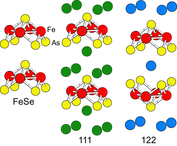
Figure 1: Typical crystal structures of iron based superconductors.

Note that all of the FeAs crystal structures shown in Fig. 1 are ion–covalent crystals. Chemical formula, say for a typical 122 system, can be written for example as Ba⁺²(Fe⁺²)₂(As^-3)₂. Here the charged FeAs layers are held by Coulomb forces from the surrounding ions. In the bulk FeSe electrically neutral FeSe layers are connected to each other by much weaker van der Waals interactions. This makes FeSe system most suitable for intercalation by various atoms and molecules that can be fairly easy introduced between the layers of FeSe. Chemistry of intercalation processes for iron chalcogenide superconductors is discussed in detail in a recent review of Ref. [Vivanco and Rodriguez, 2016].

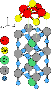
Figure 2: Crystal structure of FeSe monolayer on (001) surface of SrTiO₃with TiO₂ topmost layer.

II.1 FeSe, FeSe/STO

Bulk FeSe system has probably the simplest crystal structure among iron high-T_c superconductors. It has tetragonal structure with the space group $P$4/$nmm$ and lattice parameters $a=3.765$ Å, $c=5.518$ Å. The experimentally observed crystallographic positions are: Fe(2a) (0.0, 0.0, 0.0), Se(2c) (0.0, 0.5, z_Se), z_Se=0.2343 [Subedi et al., 2008]. In our LDA calculations of isolated FeSe layer the slab technique was used with these crystallographic parameters.

The FeSe/STO crystal structure was taken from LDA calculation with crystal structure relaxation [Zheng et al., 2013]. In slab approach FeSe monolayer was placed on three TiO₂-SrO layers to model the bulk SrTiO₃ substrate. The FeSe/STO slab crystal structure parameters used were $a=3.901$ Å, Ti-Se distance $3.13$ Å, Fe-O distance $4.43$ Å, distance between top (bottom) Se ion and the Fe ions plane is 1.41 Å (1.3 Å). Atomic positions used were: Sr – (0.5,0.5,-1.95 Å), O – (0.5,0,0), (0,0,-1.95 Å), Ti – (0,0,0).

The structure of the FeSe monolayer film on STO is shown in Fig. 2. Here the FeSe layer is directly adjacent to the surface TiO₂ layer of STO. The lattice constant within FeSe layer in a bulk samples is equal to 3.77Å, while STO has substantially greater lattice constant equal to 3.905 Å, so that the single – layer FeSe film should be noticeably stretched, as compared with the bulk FeSe. However this tension quickly disappears as the number of subsequent layers grows.

II.2 KFe₂Se₂

The ideal KFe₂Se₂ compound has tetragonal structure with the space group $I$4/$mmm$ and lattice parameters $a=3.9136$ Å and $c=14.0367$ Å. The crystallographic positions are: K(2a) (0.0, 0.0, 0.0), Fe(4d) (0.0, 0.5, 0.25), Se(4e) (0.0, 0.5, z_Se) with z_Se=0.3539 [Guo et al., 2010]. The crystal structure of K_xFe₂Se₂ is shown in Fig. 3.

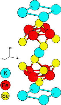
Figure 3: Ideal ($x$=1) crystal structure of 122-type of K_xFe₂Se₂ compound.

Below we compare the ARPES detected quasiparticle bands for FeSe/STO and K_xFe_2-ySe₂ and make comparison of these bands with the results of LDA+DMFT calculations for these systems, as well as for isolated FeSe layer, together with the analysis of initial LDA calculated bands [Nekrasov et al., 2016].

III Computation details

Our LDA^′ calculations [Nekrasov et al., 2012, 2013a] of KFe₂Se₂ compound were performed using the Linearized Muffin-Tin Orbitals method (LMTO) [Andersen, 1975; Gunnarsson et al., 1983; Andersen and Jepsen, 1984]. The electronic structures of FeSe monolayer and FeSe monolayer on SrTiO₃ substrate were calculated within FP-LAPW method [Blaha et al., 2016].

For DMFT part of LDA+DMFT calculations we always employed the CT-QMC impurity solver [Werner et al., 2006; Haule, 2007; Gull et al., 2011; Parcollet et al., 2015]. To define DMFT lattice problem for KFe₂Se₂ compound we used the full LDA Hamiltonian, same as in Refs. [Nekrasov et al., 2013b, c]. For isolated FeSe layer and FeSe/STO projection on Wannier functions was done for Fe-3d and Se-4p states (isolated FeSe layer) and for Fe-3d, Se-4p states and O-2p_y states from TiO₂ layer adjacent to SrTiO₃ (FeSe/STO). To this end the standard wien2wannier interface [Kuneš et al., 2010] and wannier90 projecting technique [Mostofi et al., 2008] were applied.

The DMFT(CT-QMC) computations were done at reciprocal temperature $\beta=$40 eV^-1 ($\sim$290 K) with about 10⁸ Monte-Carlo sweeps. Interaction parameters of Hubbard model were taken $U$=5.0 eV, $J$=0.9 eV for isolated FeSe and FeSe/STO and $U$=3.75 eV, $J$=0.56 eV for KFe₂Se₂ [Yi et al., 2013]. We employed the self-consistent fully-localized limit definition of the double-counting correction [Nekrasov et al., 2013a]. Thus computed values of Fe-3d occupancies and corresponding double-counting energies are $E_{dc}=18.886$ eV, $n_{d}=5.79$ (K_0.76Fe_1.72Se₂), $E_{dc}=31.63$ eV, $n_{d}=7.35$ (isolated FeSe layer), $E_{dc}=30.77$ eV, $n_{d}=7.16$ LDA+DMFT calculations of FeSe/STO were performed for doping level of 0.2 electrons per Fe ion. Chemical composition K_0.76Fe_1.72Se₂ corresponds to the total number of electrons 26.52 per unit cell which corresponds to the doping level of 1.24 holes per Fe ion. This doping level was taken for LDA^′+DMFT calculations. Moreover a number of LDA+DMFT calculations of FeSe/STO for various model parameters can be seen in the Appendix.

The LDA+DMFT spectral function maps were obtained after analytic continuation of the local self-energy $\Sigma(\omega)$ from Matsubara to real frequencies. To this end we have used the Pade approximant algorithm [Vidberg and Serene, 1977] and checked the results with the maximum entropy method [Jarrell and Gubernatis, 1996] for Green’s function G($\tau$).

IV Electronic structure of iron – selenium systems

Electronic spectrum of iron pnictides now is well understood, both from theoretical calculations based on the modern band structure theory and ARPES experiments [Sadovskii, 2008; Ishida et al., 2009; Johnston, 2010; Hirschfeld et al., 2011; Stewart, 2011; Kordyuk, 2012]. It is clear that almost all physics related to superconductivity is determined by electronic states of FeAs plane (layer), shown in Fig. 1. The spectrum of carriers in the vicinity of the Fermi level $\pm$ 0.5 eV, where superconductivity is formed, practically have only Fe-3$d$ character. The Fermi level is crossed by up to five bands (two or three hole and two electronic ones), forming a typical spectrum of a semi – metal.

In this rather narrow energy interval near the Fermi level this dispersions can be considered as parabolic [Hirschfeld et al., 2011; Kuchinskii and Sadovskii, 2010]. Most LDA+DMFT calculations [Skornyakov et al., 2009; Nekrasov et al., 2015] show that the role of electronic correlations in iron pnictides, unlike in the cuprates, is relatively insignificant. It is reduced to more or less significant effective mass renormalization of the electron and hole dispersions, as well as to general narrowing (“compression”) of the bandwidths.

The presence of the electron and hole Fermi surfaces of similar size, satisfying (approximately) the “nesting” condition plays an important role in the theories of superconducting pairing in iron arsenides based on (antiferromagnetic) spin fluctuation mechanism of pairing [Hirschfeld et al., 2011]. We shall see below that the electronic spectrum and Fermi surfaces in the Fe chalcogenides are very different from those in Fe pnictides. This raises the new problems for the understanding of microscopic mechanism of superconductivity in FeSe systems.

IV.1 A_xFe₂Se₂ system

IV.1.1 DFT/LDA results

First LDA calculations of electronic structure of the A_xFe_2-ySe₂ (A=K,Cs) system were performed soon after its experimental discovery [Nekrasov and Sadovskii, 2011; Shein and Ivanovskii, 2011]. Surprisingly enough, this spectrum was discovered to be qualitatively different from that of the bulk FeSe and spectra of practically all known systems based on FeAs. In Fig. 4 on the left we show energy bands of BaFe₂As₂ (Ba122) [Nekrasov et al., 2008] (which is the typical prototype of all FeAs systems) and those of KFe₂Se₂ [Nekrasov and Sadovskii, 2011] on the right. One can observe a significant difference in the spectra near the Fermi level.

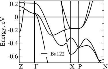
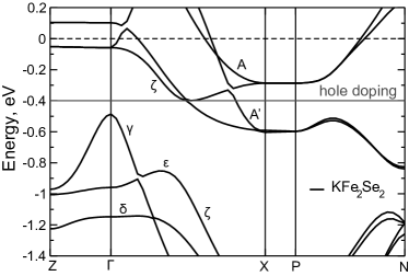
Figure 4: Left – LDA bands of Ba122 near the Fermi level ($E=$0) [Nekrasov et al., 2008], right – LDA^′ bands of KFe₂Se₂. Additional horizontal lines correspond to Fermi level of 60% hole doping [Nekrasov and Sadovskii, 2011]. The letters designate bands in the same way as in Fig. 12.

In Fig. 5 we show the calculated Fermi surfaces for K_xFe_2-ySe₂ system at various doping levels [Nekrasov and Sadovskii, 2011]. These differ significantly from the Fermi surfaces of FeAs systems — in the center of the Brillouin zone, there are only small Fermi sheets of electronic nature, while the electronic cylinders in the Brillouin zone corners are substantially larger. The shapes of the Fermi surfaces, typical for bulk FeSe and FeAs systems, can be obtained only at a much larger (apparently experimentally inaccessible) levels of the hole doping [Nekrasov and Sadovskii, 2011].

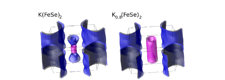
Figure 5: LDA Fermi surfaces for the stoichiometric KFe₂Se₂ (left) and at 20% hole doping (right) [Nekrasov and Sadovskii, 2011].

This shape of the Fermi surfaces in K_xFe_2-ySe₂ systems was almost immediately confirmed in ARPES experiments. For example, in Fig. 6 we show the ARPES data of Ref. [Zhao et al., 2011], which are obviously in qualitative agreement with LDA results of Refs. [Nekrasov and Sadovskii, 2011; Shein and Ivanovskii, 2011].

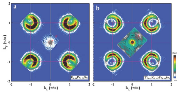
Figure 6: ARPES Fermi surfaces of K_0.68Fe_1.79Se₂ ($T_{c}$=32K) and Tl_0.45K_0.34Fe_1.84Se₂ ($T_{c}$=28K) [Zhao et al., 2011].

Note, that in this system it is clearly impossible to speak of any, even approximate, “nesting” properties of electron and hole Fermi surfaces.

IV.1.2 LDA+DMFT results

LDA+DMFT and LDA^′+DMFT calculations for K_1-xFe_2-ySe₂ system for various doping levels were performed in Refs. [Nekrasov et al., 2013b, c, 2017]. The results of these calculations can be directly compared with the ARPES data obtained in Refs. [Yi et al., 2013; Niu et al., 2016; Sunagawa et al., 2016].

It turns out that in K_1-xFe_2-ySe₂ correlation effects are quite important, leading to a noticeable change of LDA calculated dispersions. In contrast to iron arsenides, where the quasiparticle bands near the Fermi level are well defined, in the K_1-xFe_2-ySe₂ compounds in the vicinity of the Fermi level we observe much stronger suppression of the intensity of quasiparticle bands. This reflects the stronger role of correlations in this system, as compared to iron arsenides. The value of the quasiparticle renormalization (correlation narrowing) of the bands at the Fermi level is 4-5, whereas in iron arsenides this factor is only 2-3 for the same values of the interaction parameters. That can be understood in terms of $W$ – width of bare LDA Fe-3d states. As it is shown on Fig. 7 the largest bandwidth $W$=5.2 eV has isolated FeSe monolayer (red curve), then comes Ba122 (green curve) with $W$=4.8 eV, FeSe/STO (black curve) with $W$=4.3 eV. and finally the most narrow bare band has KFe₂Se₂ system (blue curve) – $W$=3.5 eV. In its turn such lowering of the $W$ can be explained by the growth of lattice constant from imlFeSe to KFe₂Se₂.

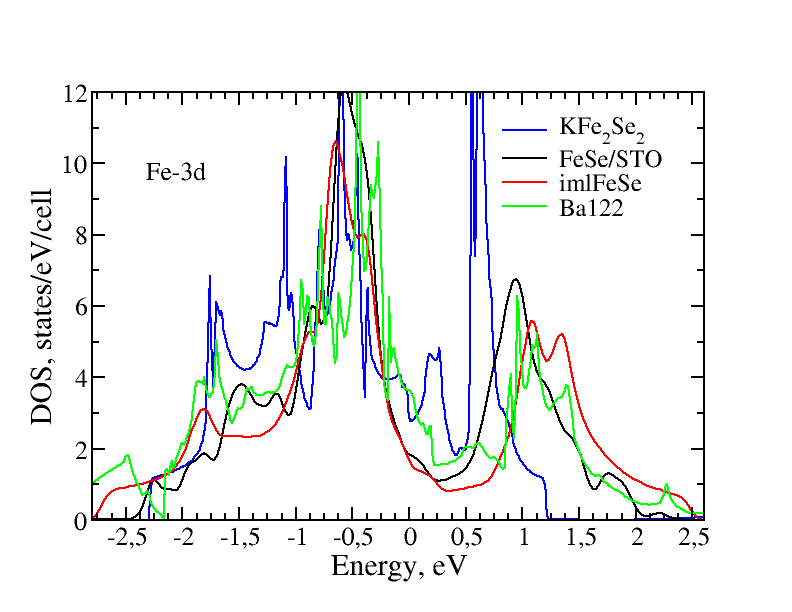
Figure 7: LDA calculated densities of states (DOS) for various iron-based superconductors: imlFeSe (red, $W$=5.2 eV), Ba122 (green, $W$=4.8 eV), FeSe/STO (black, $W$=4.3 eV), KFe₂Se₂ (blue, $W$=3.5 eV) Fermi level is at zero energy.

The results of these calculations, in general, are in good qualitative agreement with the ARPES data [Yi et al., 2013; Niu et al., 2016], which demonstrate strong damping of quasiparticles in the immediate vicinity of the Fermi level and a strong renormalization of the effective masses as compared to systems based on FeAs.

In Fig. 8 we present the comparison of LDA+DMFT spectral function maps (panel (d)) [Nekrasov et al., 2017] and ARPES data of Ref. [Sunagawa et al., 2016] (panels (a,b,c,e)) for K_xFe_2-ySe₂. Panels (a,b,c) of Fig. 8 correspond to different incident beam polarizations in ARPES experiment: $E_{s}$ – polarization in the plane parallel to the sample surface; $E_{p}$ – polarization in the plane normal to the sample surface; $E_{cir}$ – circular polarization. The use of different polarizations allows one to distinguish contributions of bands with different symmetry (see discussion in Refs. [Sunagawa et al., 2016; Nekrasov et al., 2015]). This fact is clear from the data on panels (a,b,c) of Fig. 8 where different bands are marked with Greek letters. In Fig. 8(e) we show the joint picture of all quasiparticle bands detected in ARPES [Sunagawa et al., 2016] experiment.

Now we can explain the origin of the experimental bands and their orbital composition on the basis of LDA^′ [Nekrasov et al., 2012, 2013a, 2013b, 2013c] calculations for KFe₂Se₂ (Fig. 4, right panel) and LDA^′+DMFT results of Ref. [Nekrasov et al., 2017] (Fig. 8, panel (e)). In our LDA^′+DMFT calculations the $A$ quasiparticle band near X-point corresponds to Fe-3d_xz and Fe-3d_yz states and the $A^{\prime}$ quasiparticle band near X-point is mainly formed by Fe-3d_xy states. These bands are denoted in the same way as on right panel of Fig. 4. At about -0.15 eV at the X-point there is $\omega$ quasiparticle band which is formed in our calculations due to self-energy effects only.

Thus the $A$ band is located at $\sim$ 50 meV where shallow band, typical for FeSe monolayer materials, is observed experimentally. Another shallow band $A^{\prime}$ near M-point has energy about 75 meV. The $A^{\prime}$ band might be strongly suppressed in the experiments due to its Fe-3d_xy symmetry as it is stressed by the authors of Ref. [Sunagawa et al., 2016]. So both $A$ and $A^{\prime}$ bands are just correlation renormalized LDA^′ bands (compare with right panel of Fig. 4). Similar conclusion can be given concerning the $B$ band and $B^{\prime}$ bands. Also one should note here that quasiparticle masses of the $A$ and $A^{\prime}$ bands are only slightly different. It is also important to say that $A^{\prime}$ is well defined near the Fermi level and is almost undetected near X-point (Fig. 8, panel (e)).Thus for the case of KFe₂Se₂ system we have evidently shown that purely electronic shallow $A$ and $A^{\prime}$ bands agree rather well with ARPES data [Sunagawa et al., 2016]. Moreover as we will point out later FeSe/STO bands near M-point are practically the same. So one can clearly see that such $A$ and $A^{\prime}$ band dispersions are a common feature of FeSe-based materials and probably can be resolved completely in future ARPES experiments.

Let us turn to bands around $\Gamma$-point. The $\varepsilon$ and $\delta$ bands are formed by Fe-3d${}_{3z^{2}-r^{2}}$ states. The $\varepsilon$ band is rather strongly modified in comparison with the initial LDA^′ $\varepsilon$ band (see Fig. 4, right panel), while the $\delta$ band more or less preserves its initial form. Energy location of $\varepsilon$ quasiparticle band agrees well in LDA^′+DMFT and ARPES. However, the $\delta$ band is much lower in energy in LDA^′+DMFT calculations. At the $\Gamma$-point the $\gamma$ band (which is the hybrid band of Fe-3d_xz, Fe-3d_yz and Fe-3d_xy states) in LDA^′+DMFT is above the $\varepsilon$ and $\delta$ bands in contrast with ARPES data (Fig. 8(e)). This picture is somehow inherited from the initial LDA^′ band structure (Fig. 4, right). The $\zeta$ band (Fig. 8(e)) consists in fact of two bands. The upper part (above 130 meV) of this band is formed by Fe-3d_xz and Fe-3d_yz states, while its lower part is formed by Fe-3d${}_{3z^{2}-r^{2}}$ states. In ARPES experiments this band is only partially observed around 80 meV (Fig. 8(e)), while its lower part is not distinguished experimentally from $\omega$ band [Sunagawa et al., 2016].

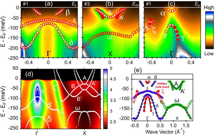
Figure 8: Panels – (a),(b),(c) ARPES data around $\Gamma$ and X-points for K_0.62Fe_1.7Se₂ [Sunagawa et al., 2016]; (d) – LDA^′+DMFT spectral function map with maxima shown by white crosses for K_0.76Fe_1.72Se₂ [Nekrasov et al., 2017]; (e) – quasiparticle bands extracted from ARPES [Sunagawa et al., 2016]. Bands of similar orbital character are marked with Greek letters on all panels. Fermi level is at zero energy.

The orbitally resolved spectral function of K_0.76Fe_1.72Se₂ is shown in Fig. 9. Here the bands are rather strongly renormalized by correlations not only by the constant scaling factor, but also because of band shapes modifications in comparison to LDA bands. Since electronic correlations are quite strong for K_0.76Fe_1.72Se₂ (because of most narrow Fe-3d bare band among considered systems, see Fig. 7) and bands are rather broadened by lifetime effects we explicitly show here the spectral function maxima positions by crosses. We can conclude that quasiparticle bands structures around the Fermi level for both compositions under discussion are rather similar.

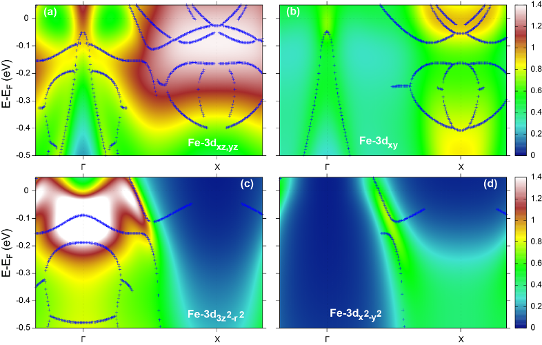
Figure 9: LDA^′+DMFT spectral function map [Nekrasov et al., 2017] for different Fe-3d orbitals of K_0.76Fe_1.72Se₂: (a) – Fe-3d_xz and Fe-3d_yz, (b) – Fe-3d_xy, (c) – Fe-3d${}_{3z^{2}-r^{2}}$, (d) – Fe-3d${}_{x^{2}-y^{2}}$. Maxima of the spectral density are shown with crosses. Fermi level is zero energy.

The overall agreement between ARPES and LDA^′+DMFT results for K_0.76Fe_1.72Se₂ system is rather satisfactory and allows one to identify the orbital composition of different bands detected in the experiment. However $\alpha$ and $\beta$ bands found in ARPES are not observed in our LDA^′+DMFT calculated spectral function maps. More so there are no obvious candidates for these bands within the LDA^′ band structure (Fig. 4, right). Thus the origin of experimentally observed $\alpha$ and $\beta$ quasiparticle bands (if there are some) remains at present unclear.

IV.2 FeSe monolayer films

IV.2.1 DFT/LDA results

The results of our LDA calculations [Nekrasov et al., 2016] of the spectrum for the isolated FeSe monolayer together with FeSe layer on STO substrate are shown in Fig. 10. This spectrum has the form typical for FeAs based systems and bulk FeSe as discussed in detail above. However ARPES experiments [Liu et al., 2012; Lee et al., 2014a; Zhao et al., 2016] are in striking disagreement with these results. Actually, in FeSe monolayers on STO only electron – like Fermi surface sheets are observed around the $M$ – points of the Brillouin zone, while hole – like sheets, centered around the $\Gamma$ – point (in the center of the zone), are just absent. An example of such data is shown in Fig. 11 (a) [Liu et al., 2012]. Similarly to intercalated FeSe systems there is no place for “nesting” of Fermi surfaces – there are just no surfaces to “nest”!

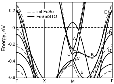
Figure 10: LDA band dispersions of paramagnetic isolated FeSe monolayer (dashed line) and paramagnetic FeSe/STO (solid line). The letters designate bands in the same way as in Fig. 12. The Fermi level $E_{F}$ is at zero energy.

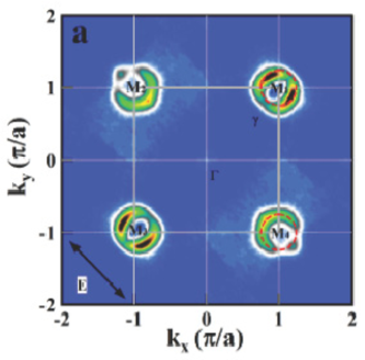
Figure 11: Experimental ARPES Fermi surface of FeSe monolayer [Liu et al., 2012; Lee et al., 2014a].

In order to explain this contradiction between ARPES experiments [Liu et al., 2012] and band structure calculations reflected in the absence of hole – like cylinders at the $\Gamma$ – point, one can suppose it to be the consequence of FeSe/STO monolayer stretching due to mismatch of lattice constants of the bulk FeSe and STO. We have studied this problem by varying the lattice parameter $a$ and Se height $z_{Se}$ in the range $\pm 5\%$ around the bulk FeSe parameters with the account of lattice relaxation. The conclusion was that the changes of lattice parameters do not lead to qualitative changes of FeSe Fermi surfaces and the hole – cylinders in the $\Gamma$ – point always remain more or less intact.

However, there is another rather simple possible explanation for the absence of hole – like cylinders and the observed Fermi surfaces can be obtained assuming that the system is doped by electrons. The Fermi level has to be moved upwards in energy by the value of $\sim$ 0.2 - 0.25 eV, corresponding to the doping level of 0.15 - 0.2 electron per Fe ion.

The nature of this doping, strictly speaking, is not fully understood. There is a common belief that it is associated with the formation of oxygen vacancies in the SrTiO₃ substrate (in the topmost layer of TiO₂), occurring during the various technological steps used during film preparation, such as annealing, etching, etc. It should be noted that the formation of the electron gas at the interface with the SrTiO₃ is rather widely known phenomenon, which was studied for a long time [Fu et al., 2016]. At the same time, for FeSe/STO system this issue was not analyzed in detail and remains unexplained (see, however, recent Refs. [Zhou and Millis, 2016; Chen et al., 2016].

IV.2.2 LDA+DMFT results

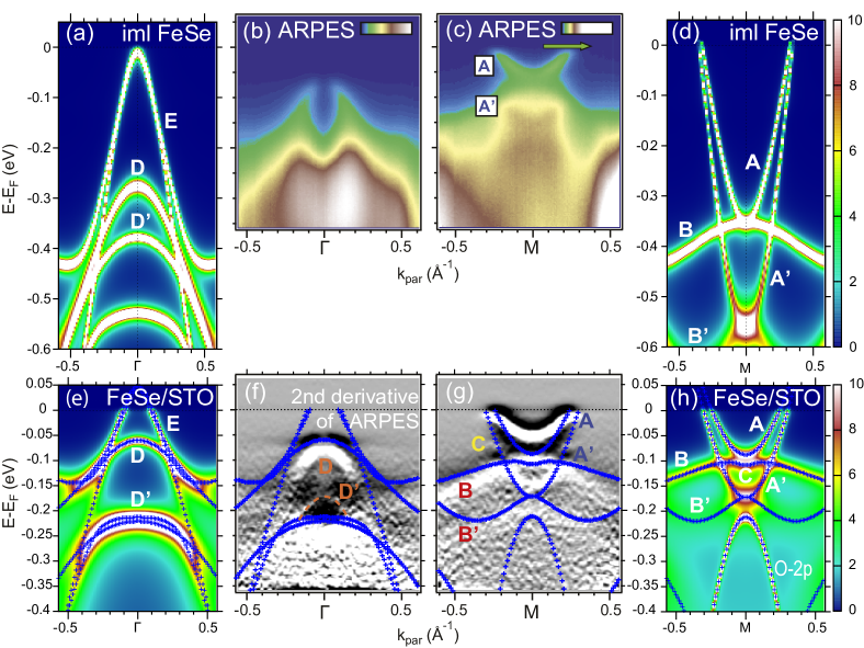
Figure 12: (a), (d) panels – LDA+DMFT spectral function maps of isolated FeSe monolayer [Nekrasov et al., 2017] and (b),(c) – experimental ARPES data around $\Gamma$ and M points and (f), (g) corresponding second derivatives of ARPES data for FeSe/STO [Lee et al., 2014b] with LDA+DMFT spectral function maxima shown with crosses; (e), (h) – LDA+DMFT spectral function maps [Nekrasov et al., 2017] with maxima shown with crosses for FeSe/STO. To mark similar features of experimental and theoretical spectral function maps $A,B,C,D,E$ letters are used (the same as in Fig. 10 for LDA bands). Fermi level is at zero energy.

In Fig. 12 we compare our theoretical LDA+DMFT results [Nekrasov et al., 2017], shown on panels (a,d,e,h), with experimental ARPES data [Lee et al., 2014b], shown on panels (b,c,f,g). LDA+DMFT spectral function maps of isolated FeSe monolayer are shown in Fig. 12(a) and Fig. 12(d) at $\Gamma$ and M points respectively. For FeSe/STO LDA+DMFT calculated spectral function maps are shown on (e), (h) panels at $\Gamma$ and M points. The obtained LDA bandwidth $W$ of Fe-3d band in isolated FeSe monolayer it is 5.2 eV, which is much larger than 4.3 eV obtained for FeSe/STO. This is due to the lattice constant $a$ expanded from $a=3.765$ Å to $a=3.901$ Å in going from isolated FeSe monolayer to FeSe/STO (see Fig. 7). Thus for the same interaction strength and doping levels LDA+DMFT calculations demonstrate substantially different band narrowing due to correlation effects. It is a factor of 1.5 in isolated FeSe monolayer (same as bulk FeSe) and a factor of 3 in FeSe/STO. Thus, we may conclude that FeSe/STO system is more correlated as compared with the bulk FeSe or isolated FeSe layer with respect to $U/W$ ratio.

Most of features observed in the ARPES experiments (Fig.  12, panels (f),(g)) can be identified with our calculated LDA+DMFT spectral function maps (Fig.  12, panels (e),(h)). The experimental quasiparticle bands around M-point marked by $A$, $B$ and $C$ (Fig. 12(g,h)) correspond mainly to Fe-3d_xz and Fe-3d_yz states, while the $A^{\prime}$ and $B^{\prime}$ quasiparticle bands have predominantly Fe-3d_xy character.

The shallow band at M-point originates from LDA Fe-3d_xz and Fe-3d_yz bands (see also Fig. 10) compressed by electronic correlations. Trying to achieve the better agreement with experiments we also examined the reasonable increase of Coulomb interaction within LDA+DMFT and the different doping levels, but these have not produced the significant improvement of our results. Corresponding LDA+DMFT spectral function maps for FeSe/STO system are presented in the Appendix with variation of only one of model parameters $U$, $J$ or occupancy $n$ while the other two remain fixed.

The $C$ quasiparticle band near M-point appeared due to lifting of degeneracy of Fe-3d_xz and Fe-3d_yz bands (which is in contrast to isolated FeSe layer, see panel Fig. 12(d)). The origin of this band splitting is directly related to the $z_{Se}$ height difference below and above Fe ions plane due to the presence of interface with SrTiO₃.

The appearance of $A^{\prime}$ (and in some works $B^{\prime}$) band in FeSe/STO is usually attributed to forward scattering interaction with 100 meV optical phonon of STO substrate [Lee et al., 2014b; Gor’kov, 2016a, b; Rademaker et al., 2016; Wang et al., 2016a]. Further in the Section V we will provide some estimates of such electron-optical phonon coupling strength which in fact is obtained to be exponentially small for the case of FeSe/STO making this scenario of the “replica” band formation quite questionable. Our calculations clearly show that $A^{\prime}$ band of purely electronic nature appears almost exactly at the energies of the so called “replica” band with no reference to phonons. Quasiparticle masses (as listed in Tab. 1 of the Appendix) of $A$ and $A^{\prime}$ bands differ from each other not more then by 10%. If we concentrate our attention close to M-point the shapes of $A$ and $A^{\prime}$ bands are almost the same within the accuracy of experimental data. Let us note here that equal shapes (or the same quasiparticle masses) of $A$ and $A^{\prime}$ bands is a keypoint of phenomenological “replica” band description in Refs. [Lee et al., 2014b; Rademaker et al., 2016] One should say here that the $B^{\prime}$ band is well seen in our LDA+DMFT results (Fig.  12, panels (g),(h)) also without introducing of any electron-phonon coupling. In contrast to K_0.76Fe_1.72Se₂ case in FeSe/STO system the $A^{\prime}$ band is well detected in the ARPES near M-point while near Fermi level it is strongly suppressed. This may be due to some matrix elements effects as discussed in Refs. [Sunagawa et al., 2016; Watson et al., 2015] and references therein, as well as in Refs. [Nekrasov et al., 2015; Sunagawa et al., 2016] in the context of NaFeAs compound. Again, similar to the K_0.76Fe_1.72Se₂ case we propose that $A^{\prime}$ and $B^{\prime}$ bands are common feature of FeSe-based materials and should be experimentally observed irrespective of the electron-phonon scenario of the “replica” band.

Thus, for FeSe/STO system we observe the general agreement between the results of LDA+DMFT calculations of Ref. [Nekrasov et al., 2017] (Fig.  12(h)) and ARPES data [Lee et al., 2014b] (Fig. 12(g)) on semi-quantitative level with respect to relative positions of quasiparticle bands. Note that the Fermi surfaces formed by the $A$ and $A^{\prime}$ bands in our LDA+DMFT calculations are nearly the same as the Fermi surface observed at M-point by ARPES.

Actually, all quasiparticle bands in the vicinity of M-point can be well represented as LDA bands compressed by a factor of 3 due to electronic correlations. This fact is clearly supported by our calculated LDA band structure shown on Fig. 10, where different bands are marked by letters identical to those used in Fig. 12.

Near the M-point we also observe the O-2p_y band (in the energy interval below -0.2 eV (Fig. 12(h)) originating from TiO₂ layer adjacent to FeSe. Due to doping level used this O-2p_y band goes below the Fermi level in contrast to LDA picture shown in Fig. 10 where O-2p_y band crosses the Fermi level and forms hole pocket. This observation rules out possible nesting effects between these bands which might be expected from LDA results [Nekrasov et al., 2016].

Now let us discuss the bands around the $\Gamma$-point, which are shown on panels (a,b,e,f) of Fig. 12. Here the situation is much somehow simpler than in the case of M-point. One can see here only two bands observed in the experiment (Fig. 12(f)). The $D$ quasiparticle band has predominantly Fe-3d_xy character, while the $D^{\prime}$ quasiparticle band originates from Fe-3d${}_{3z^{2}-r^{2}}$ states. The relative locations of LDA+DMFT calculated $D$ and $D^{\prime}$ bands are quite similar to the ARPES data.

Main discrepancy of LDA+DMFT results and ARPES data here is the $E$ band shown in Fig. 12(e) which is not observed in the ARPES. This band corresponds to a hybridized band of Fe-3d_xz, Fe-3d_yz and Fe-3d_xy states. In principle some traces of this band can be guessed in the experimental data of Fig. 12(f) around -0.17 eV and near the $k$-point 0.5. Surprisingly these are missed in the discussion of Ref. [Lee et al., 2014b]. Actually, the ARPES signal from $E$ band can be weakened because of sizable Fe-3d_xy contribution [Sunagawa et al., 2016; Watson et al., 2015; Nekrasov et al., 2015; Sunagawa et al., 2016] and thus might be indistinguishable from $D$ band. Also one can imagine that for stronger band renormalization the $E$ band becomes more flat and might merge with $D$ band.

To show different Fe-3d orbitals contribution to LDA+DMFT spectral functions of we present here the corresponding orbital resolved spectral function maps. In Fig. 13 it is clearly seen that the quasiparticle bands of isolated FeSe monolayer are well defined and have similar shape to the LDA bands except correlation narrowing by the same constant factor for all bands. The quasiparticle bands of FeSe/STO are more broad but still well defined. The main contribution to spectral function near the Fermi level belongs to Fe-3d_xz, Fe-3d_yz and Fe-3d_xy states both for the isolated FeSe layer and FeSe/STO.

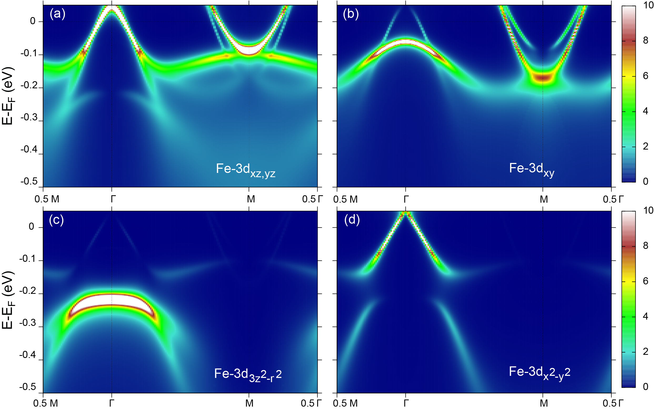
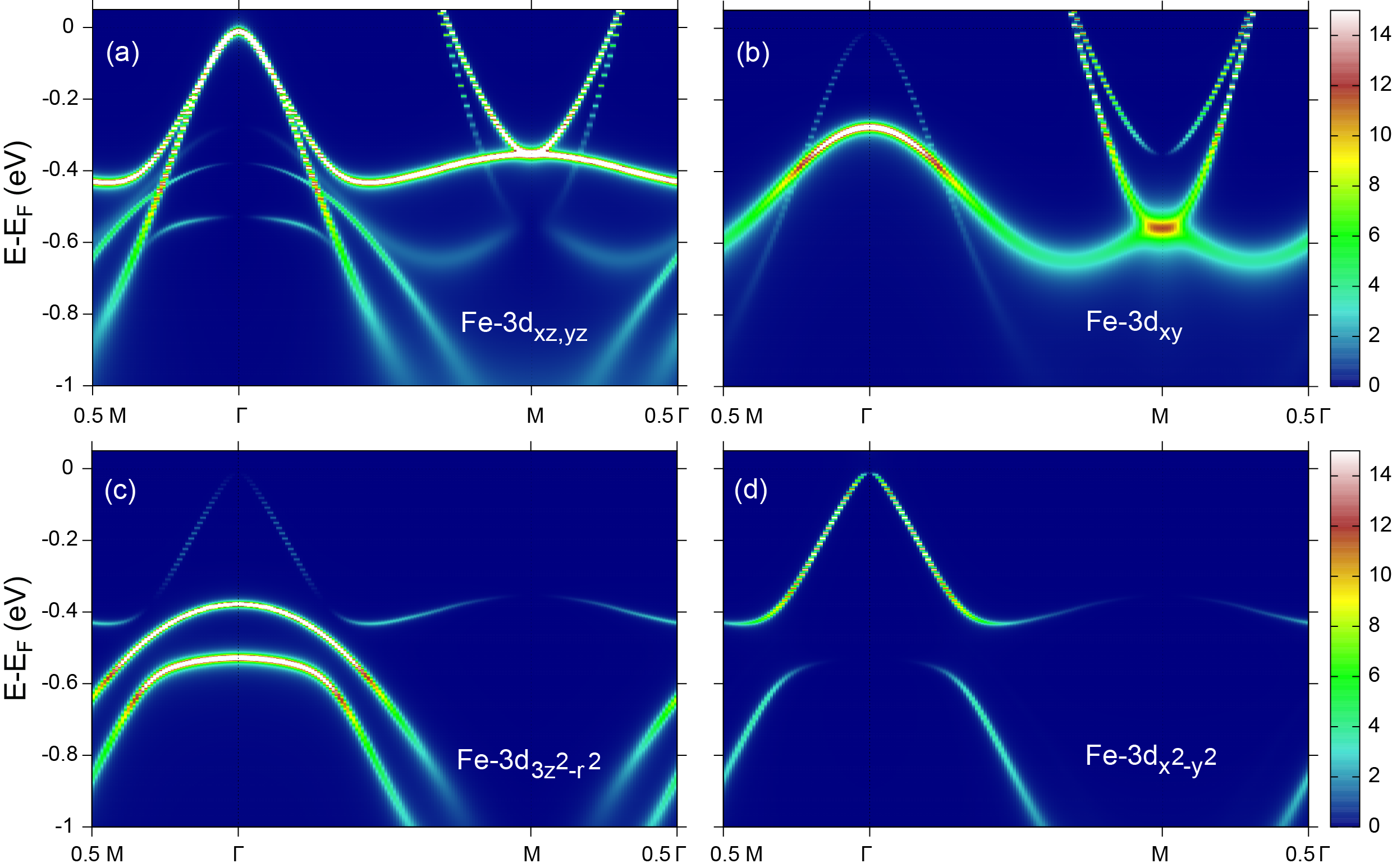
Figure 13: LDA+DMFT spectral function maps [Nekrasov et al., 2017] for different Fe-3d orbitals of FeSe monolayer on SrTiO₃ substrate (top) and isolated FeSe monolayer (bottom): (a) – Fe-3d_xz and Fe-3d_yz, (b) – Fe-3d_xy, (c) – Fe-3d${}_{3z^{2}-r^{2}}$, (d) – Fe-3d${}_{x^{2}-y^{2}}$. Fermi level is at zero energy.

V “Replica” band and electron – optical phonon coupling in FeSe/STO

As we mentioned earlier, the most popular explanation of the appearance of the “replica” band around the M-point in FeSe/STO is related to FeSe electrons interaction with $\sim$100 meV optical phonons in STO. This idea was first proposed in Ref. [Lee et al., 2014b], where it was experimentally observed for the first time. In this work (see also Ref. [Kulić and Dolgov, 2017]) it was also shown that due to the peculiar nature of electron – optical phonon interactions at FeSe/STO interface, the appropriate coupling constant is exponentially suppressed with transferred momentum and can be written as:

$$g({\bf q})=g_{0}\exp(-|{\bf q}|/q_{0})$$ (1)

where typically $q_{0}\sim 0.1\frac{\pi}{a}\ll p_{F}$ ($a$ is the lattice constant and $p_{F}$ is the Fermi momentum), leading to the picture of nearly forward scattering of electrons by optical phonons. This picture was further developed in model approach of Refs. [Rademaker et al., 2016; Wang et al., 2016a] where it was shown, that such coupling can also lead to rather significant increase of the temperature of superconducting transition $T_{c}$ in accordance with earlier ideas developed by Dolgov and Kulić [Danylenko, O. V. et al., 1999; Kulić, 2004] (see also the review in [Sadovskii, 2016]). However, the significant effect here can be achieved only for the case of large enough effective coupling of electrons with such forward scattering phonons.

The standard dimensionless electron – phonon coupling constant of Eliashberg theory for the case of optical (Einstein) phonon at FeSe/STO interface can be written as ($N$ is the number of lattice sites) [Allen, 1972]:

$$\lambda=\frac{2}{N\Omega_{0}}\frac{\sum_{{\bf p},{\bf q}}|g({\bf q})|^{2}\delta{(\epsilon{(\bf p)}-\mu)}\delta(\epsilon{(\bf p+q)})-\mu-\Omega_{0})}{\sum_{\bf p}\delta(\epsilon({\bf p})-\mu)},$$ (2)

where we explicitly introduced (optical) phonon frequency $\Omega_{0}$ in $\delta$-function, which is usually neglected in adiabatic approximation. In FeSe/STO system we actually have $\Omega_{0}>E_{F}$, so that it is obviously should be kept finite.

For simple estimates we can assume the linearized spectrum of electrons ($v_{F}$ is Fermi velocity): $\xi_{p}\equiv\epsilon{(\bf p)}-\mu\approx v_{F}(|{\bf p}|-p_{F})$ so that all calculations can be done explicitly in analytic form. Now using (1) in (2) for two-dimensional case we can write:

$$\lambda=\frac{2}{\Omega_{0}}g_{0}^{2}\int_{-\infty}^{\infty}d\xi_{p}\delta(\xi_{p})\int\frac{d^{2}q}{(2\pi)^{2}}\exp{\left(-\frac{2q}{q_{0}}\right)}\delta(\xi_{p}-\Omega_{0}+v_{F}q\cos\phi)=$$

$$=\frac{2g_{0}^{2}}{\Omega_{0}}\frac{a^{2}}{4\pi^{2}}\int_{0}^{\infty}dqq\exp\left(-\frac{2q}{q_{0}}\right)\int_{0}^{2\pi}d\phi\delta(v_{F}q\cos\phi-\Omega_{0}),$$ (3)

Then, after the direct calculation of all integrals, we obtain:

$$\lambda=\frac{g_{0}^{2}a^{2}}{\pi^{2}v_{F}^{2}}K_{1}\left(\frac{2\Omega_{0}}{v_{F}q_{0}}\right)$$ (4)

where $K_{1}(x)$ is Bessel function of imaginary argument (McDonald function). Using the well known asymptotic behavior of $K_{1}(x)$ and dropping some irrelevant constants we get:

$$\lambda\sim\lambda_{0}\frac{q_{0}}{4\pi p_{F}},$$ (5)

for $\frac{\Omega_{0}}{v_{F}q_{0}}\ll 1$, and

$$\lambda\sim\lambda_{0}\frac{\Omega_{0}}{\pi\varepsilon_{F}}\sqrt{\frac{v_{F}q_{0}}{\Omega_{0}}}\exp\left(-\frac{2\Omega_{0}}{v_{F}q_{0}}\right),$$ (6)

for $\frac{\Omega_{0}}{v_{F}q_{0}}\gg 1$. Here we introduced the standard dimensionless electron – phonon coupling constant as:

$$\lambda_{0}=\frac{2g_{0}^{2}}{\Omega_{0}}N(0).$$ (7)

where $N(0)$ is the density of states at the Fermi level per one spin projection.

Now it becomes obvious that the pairing constant is exponentially suppressed for $\frac{\Omega_{0}}{v_{F}q_{0}}>1$, which is typical for FeSe/STO interface, where $\Omega_{0}>E_{F}\gg v_{F}q_{0}$ [Sadovskii, 2016], making the appearance of the “replica” band and $T_{c}$ enhancement due to coupling of FeSe electrons with optical phonons of STO quite improbable. Similar conclusions were reached from from first principles calculations of Ref. [Wang et al., 2016b] and the analysis of screening of electron – phonon interactions at FeSe/STO interface in Ref. [Zhou and Millis, 2017].

As we have seen above, our LDA+DMFT calculations of FeSe/STO system produced entirely different explanation for the origin of the “replica” band not related to electron – phonon interactions.

VI Conclusions

Our LDA+DMFT results for FeSe monolayer materials such as K_xFe₂Se₂ and FeSe/STO provide the scenario of formation of puzzling shallow bands at the M-point due to correlation effects on Fe-3d states only. The detailed analysis of ARPES detected quasiparticle bands and LDA+DMFT results shows that the closer to the Fermi level shallow band (at about 50 meV) is formed by the degenerate Fe-3d_xz and Fe-3d_yz bands renormalized by correlations. Moreover, second shallow band (at about 150 meV) can be reasonably understood as simply correlation renormalized LDA Fe-3d_xy band and appears almost at the same energies as the so called “replica” band observed in ARPES for FeSe/STO, usually attributed to electron interactions with optical phonons of STO. The influence of STO substrate is reduced only to the removal of degeneracy of Fe-3d_xz and Fe-3d_yz bands in the vicinity of M-point. In the case of K_xFe_2-ySe₂ most of ARPES detected bands can also be expressed as correlation renormalized Fe-3d LDA bands. Thus we conclude that such rather unusual band structure near Fermi level with several electron-like shallow bands is a common feature of FeSe monolayer materials and apparently can be fully resolved in future ARPES experiments.

In principle, optical phonon mediated “replica” band might coincide with demonstrated by us purely electronic shallow band if the possibility of sufficiently strong electron-optical phonon coupling would be demonstrated. Our estimates of such coupling strength show that it appears to be exponentially small for the FeSe/STO case.

Correlation effects alone are apparently unable to eliminate completely the hole – like Fermi surface at the $\Gamma$-point, which is not observed in most ARPES experiments on FeSe/STO system.

*

Appendix A LDA+DMFT spectral function maps of FeSe/STO system for various model parameters

In this Appendix we show the LDA+DMFT spectral function maps for FeSe/STO system for various model parameters $U$, $J$ or occupancy $n$ while other two remains fixed.

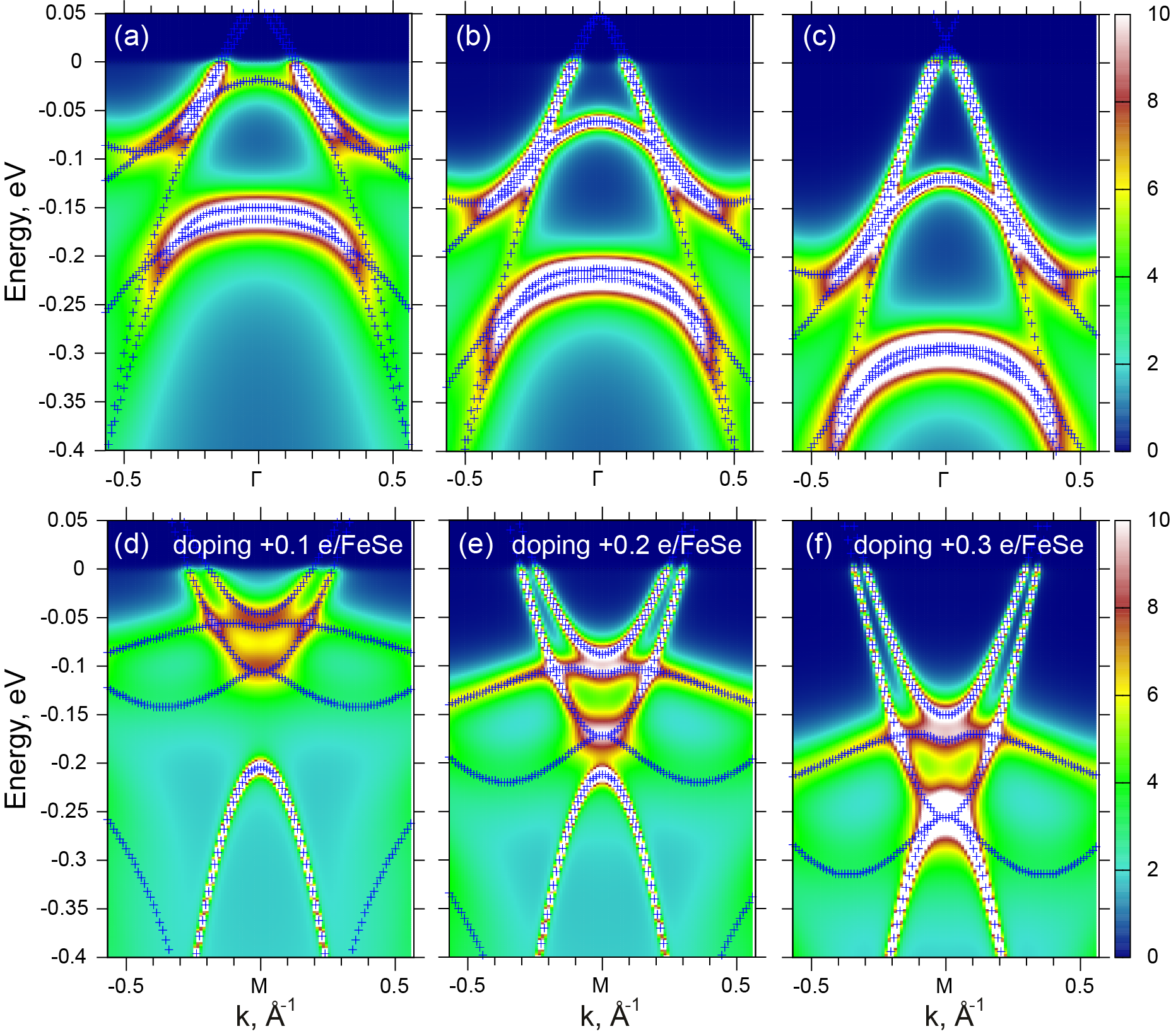
Figure 14: LDA+DMFT spectral function map of FeSe/STO for different electron doping levels (per Fe ion) for U=5.0 eV and J=0.9 eV: +0.1e, +0.2e, +0.3e (from left to right) near $\Gamma$ (upper line) and M high symmetry points (lower line). Fermi level is at zero energy.

In Fig. 14 we present doping dependence of the LDA+DMFT spectral function map of FeSe monolayer on SrTiO₃ substrate (FeSe/STO) For U=5 eV and J=0.8 eV. We assumed here three doping levels: +0.1, +0.2 (discussed in the main part of the paper) and +0.3 per Fe ion. In general such electron doping leads to a more or less rigid band shift. However with electron doping growth the correlation strength decreases as can be seen in the upper part of the Table 1. Especially correlations are weakened for t_2g orbitals – nearly twice weaker. It is well known behavior for iron-based superconductors [de’ Medici et al., 2014]. One should note here that the doping +0.3e almost vanish Fermi surface sheets in the $\Gamma$-point (see right column of the Fig. 14 on the top line) as it is observed in the ARPES (see Fig. 6. But at this doping agreement between LDA+DMFT and ARPES bands is much worth in contrast to +0.2e doping discussed above.

The Coulomb interaction dependence of the LDA+DMFT spectral function maps of FeSe/STO is shown on Fig. 15. There are three cases U=4.0 eV, U=5.0 eV and U=6.0 eV. As it is expected increase of U gives rise to correlations (see middle part of the Table 1). Such evaluation of U leads to a more less uniform bands compression. The best agreement with ARPES detected bands is found at U=5 as shown in the paper.

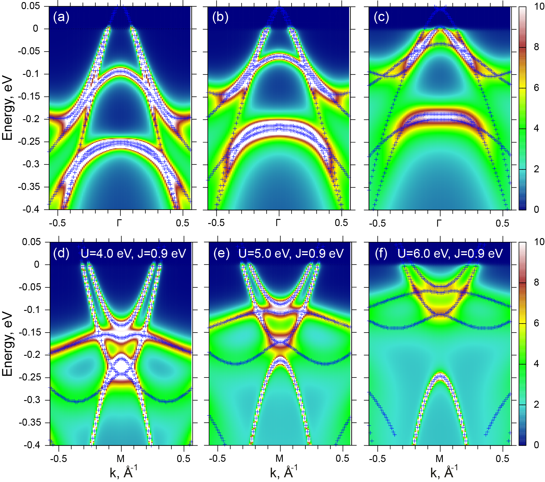
Figure 15: LDA+DMFT spectral function map of FeSe/STO for different values of U for n=+0.2e and J=0.9 eV: 4 eV, 5 eV and 6 eV (from left to right) near $\Gamma$ (upper line) and M high symmetry points (lower line). Fermi level is at zero energy.

Perhaps the most drastic effect on LDA+DMFT results of FeSe/STO produces change of the Hund’s coupling value J. In some sense it is clear since iron-based superconductors in common belief are so called “Hund’s metals” [Yin et al., 2011]. In Fig. 15 we draw Hund’s coupling dependence of the LDA+DMFT spectral function map for J=0.7 eV, 0.8 eV and 0.9 eV. In the case of J growth quasiparticle bands compression is even more evident in comparison with U evaluation (Fig. 15). However mass renormalization changes approximately by a factor of 2 (see lower part of the Table 1) similar to those of U or n variation.

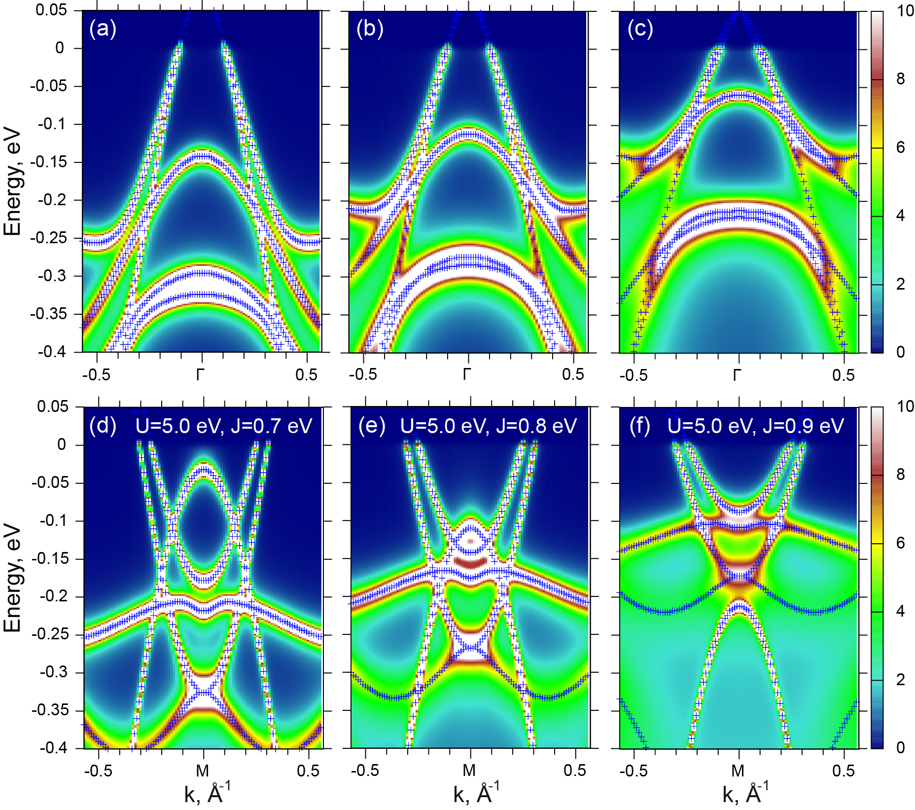
Figure 16: LDA+DMFT spectral function map of FeSe/STO for different values of J for n=+0.2e and U=5 eV: 0.7 eV, 0.8 eV and 0.9 eV (from left to right) near $\Gamma$ (upper line) and M high symmetry points (lower line). Fermi level is at zero energy.

Table 1: LDA+DMFT obtained mass renormalization values for FeSe/STO system for various model parameters U,J and n for different Fe-3d orbitals.

U=5.0 eV, J=0.9 eV(fixed)	d${}_{x^{2}-y^{2}}$	dyz	d${}_{3z^{2}-r^{2}}$	dxz	dxy
+0.1 e/FeSe	2.47	4.25	2.36	4.04	4.32
+0.2 e/FeSe	2.03	3.07	2.04	2.93	3.12
+0.3 e/FeSe	1.84	2.42	1.83	2.33	2.47
+0.2 e/FeSe, J=0.9 eV (fixed)
U=4.0 eV	1.71	2.29	1.74	2.21	2.34
U=5.0 eV	2.03	3.07	2.04	2.93	3.12
U=6.0 eV	2.74	5.11	2.57	4.84	5.14
+0.2 e/FeSe, U=5.0 eV (fixed)
J=0.7 eV	1.49	1.73	1.56	1.69	1.75
J=0.8 eV	1.63	2.05	1.70	1.99	2.08
J=0.9 eV	2.03	3.07	2.04	2.93	3.12

Finally one can say that rather moderate change of model parameters for the FeSe/STO system can produce quite drastic influence on its electronic properties.

References

- Sadovskii (2008) M. V. Sadovskii, Physics-Uspekhi 51, 1201 (2008), [Usp. Fiz. Nauk 2008, 178, 1243-1271].
- Ishida et al. (2009) K. Ishida, Y. Nakai, and H. Hosono, Journal of the Physical Society of Japan 78, 062001 (2009).
- Johnston (2010) D. C. Johnston, Advances in Physics 59, 803 (2010).
- Hirschfeld et al. (2011) P. J. Hirschfeld, M. M. Korshunov, and I. I. Mazin, Reports on Progress in Physics 74, 124508 (2011).
- Stewart (2011) G. R. Stewart, Reviews of Modern Physics 83, 1589 (2011).
- Kordyuk (2012) A. A. Kordyuk, Low Temperature Physics 38, 888 (2012), [Fizika Nizkikh Temperatur 2012, 38, 1119].
- Mizuguchi and Takano (2010) Y. Mizuguchi and Y. Takano, Journal of the Physical Society of Japan 79, 102001 (2010).
- Sadovskii et al. (2012) M. Sadovskii, E. Kuchinskii, and I. Nekrasov, Journal of Magnetism and Magnetic Materials 324, 3481 (2012), fifth Moscow international symposium on magnetism.
- Nekrasov and Sadovskii (2014) I. A. Nekrasov and M. V. Sadovskii, JETP Letters 99, 598 (2014), [Pis’ma Zh. Eksp. Teor. Fiz. 2014, 99, 687].
- Guo et al. (2010) J. Guo, S. Jin, G. Wang, S. Wang, K. Zhu, T. Zhou, M. He, and X. Chen, Phys. Rev. B 82, 180520 (2010).
- Yan et al. (2012) Y. J. Yan, M. Zhang, A. F. Wang, J. J. Ying, Z. Y. Li, W. Qin, X. G. Luo, J. Q. Li, J. p. Hu, and X. H. Chen, Scientific Reports 2 (2012), 10.1038/srep00212.
- Krzton-Maziopa et al. (2016) A. Krzton-Maziopa, V. Svitlyk, E. Pomjakushina, R. Puzniak, and K. Conder, Journal of Physics: Condensed Matter 28, 293002 (2016).
- Hatakeda et al. (2013) T. Hatakeda, T. Noji, T. Kawamata, M. Kato, and Y. Koike, Journal of the Physical Society of Japan 82, 123705 (2013).
- Burrard-Lucas et al. (2013) M. Burrard-Lucas, D. G. Free, S. J. Sedlmaier, J. D. Wright, S. J. Cassidy, Y. Hara, A. J. Corkett, T. Lancaster, P. J. Baker, S. J. Blundell, and S. J. Clarke, Nature Materials 12, 15 (2013).
- Lu et al. (2014) X. F. Lu, N. Z. Wang, H. Wu, Y. P. Wu, D. Zhao, X. Z. Zeng, X. G. Luo, T. Wu, W. Bao, G. H. Zhang, F. Q. Huang, Q. Z. Huang, and X. H. Chen, Nature Materials 14, 325 (2014).
- Pachmayr et al. (2015) U. Pachmayr, F. Nitsche, H. Luetkens, S. Kamusella, F. Brückner, R. Sarkar, H.-H. Klauss, and D. Johrendt, Angewandte Chemie International Edition 54, 293 (2015).
- Wang et al. (2012) Q.-Y. Wang, Z. Li, W.-H. Zhang, Z.-C. Zhang, J.-S. Zhang, W. Li, H. Ding, Y.-B. Ou, P. Deng, K. Chang, J. Wen, C.-L. Song, K. He, J.-F. Jia, S.-H. Ji, Y.-Y. Wang, L.-L. Wang, X. Chen, X.-C. Ma, and Q.-K. Xue, Chinese Physics Letters 29, 037402 (2012).
- Ge et al. (2014) J.-F. Ge, Z.-L. Liu, C. Liu, C.-L. Gao, D. Qian, Q.-K. Xue, Y. Liu, and J.-F. Jia, Nature Materials 14, 285 (2014).
- Miyata et al. (2015) Y. Miyata, K. Nakayama, K. Sugawara, T. Sato, and T. Takahashi, Nature Materials 14, 775 (2015).
- Zhou et al. (2016) G. Zhou, D. Zhang, C. Liu, C. Tang, X. Wang, Z. Li, C. Song, S. Ji, K. He, L. Wang, X. Ma, and Q.-K. Xue, Applied Physics Letters 108, 202603 (2016).
- Peng et al. (2014) R. Peng, H. C. Xu, S. Y. Tan, H. Y. Cao, M. Xia, X. P. Shen, Z. C. Huang, C. Wen, Q. Song, T. Zhang, B. P. Xie, X. G. Gong, and D. L. Feng, Nature Communications 5, 5044 (2014).
- Ding et al. (2016) H. Ding, Y.-F. Lv, K. Zhao, W.-L. Wang, L. Wang, C.-L. Song, X. Chen, X.-C. Ma, and Q.-K. Xue, Phys. Rev. Lett. 117, 067001 (2016).
- Song et al. (2011) C.-L. Song, Y.-L. Wang, Y.-P. Jiang, Z. Li, L. Wang, K. He, X. Chen, X.-C. Ma, and Q.-K. Xue, Physical Review B 84 (2011), 10.1103/PhysRevB.84.020503.
- Liu et al. (2015) X. Liu, L. Zhao, S. He, J. He, D. Liu, D. Mou, B. Shen, Y. Hu, J. Huang, and X. J. Zhou, Journal of Physics: Condensed Matter 27, 183201 (2015).
- Sadovskii (2016) M. V. Sadovskii, Physics-Uspekhi 59, 947 (2016), [Usp. Fiz. Nauk 2016, 186, 1035].
- Vivanco and Rodriguez (2016) H. K. Vivanco and E. E. Rodriguez, Journal of Solid State Chemistry 242, Part 2, 3 (2016), solid State Chemistry of Energy-Related Materials.
- Subedi et al. (2008) A. Subedi, L. Zhang, D. J. Singh, and M. H. Du, Physical Review B 78 (2008), 10.1103/PhysRevB.78.134514.
- Zheng et al. (2013) F. Zheng, Z. Wang, W. Kang, and P. Zhang, Scientific Reports 3, 2213 (2013).
- Nekrasov et al. (2016) I. A. Nekrasov, N. S. Pavlov, M. V. Sadovskii, and A. A. Slobodchikov, Low Temperature Physics 42, 891 (2016), [Fizika Nizkikh Temperatur 2016, 42, 1137].
- Nekrasov et al. (2012) I. A. Nekrasov, V. S. Pavlov, and M. V. Sadovskii, JETP Letters 95, 581 (2012), [Pis’ma v ZhETF 2015, 95, 659].
- Nekrasov et al. (2013a) I. A. Nekrasov, N. S. Pavlov, and M. V. Sadovskii, Journal of Experimental and Theoretical Physics 116, 620 (2013a), [Zh. Eksp. Teor. Fiz. 2013, 143, 713].
- Andersen (1975) O. K. Andersen, Phys. Rev. B 12, 3060 (1975).
- Gunnarsson et al. (1983) O. Gunnarsson, O. Jepsen, and O. K. Andersen, Phys. Rev. B 27, 7144 (1983).
- Andersen and Jepsen (1984) O. K. Andersen and O. Jepsen, Phys. Rev. Lett. 53, 2571 (1984).
- Blaha et al. (2016) P. Blaha, K. Schwarz, G. K. H. Madsen, D. Kvasnicka, and J. Luitz, An Augmented Plane Wave + Local Orbitals Program for Calculating Crystal Properties (Vienna University of Technology, Institute of Materials Chemistry, Getreidemarkt 9/165-TC, A-1060 Vienna, Austria, 2016) wIEN2k 16.1 (Release 12/12/2016) ISBN 3-9501031-1-2.
- Werner et al. (2006) P. Werner, A. Comanac, L. de’ Medici, M. Troyer, and A. J. Millis, Phys. Rev. Lett. 97, 076405 (2006).
- Haule (2007) K. Haule, Phys. Rev. B 75, 155113 (2007).
- Gull et al. (2011) E. Gull, A. J. Millis, A. I. Lichtenstein, A. N. Rubtsov, M. Troyer, and P. Werner, Rev. Mod. Phys. 83, 349 (2011).
- Parcollet et al. (2015) O. Parcollet, M. Ferrero, T. Ayral, H. Hafermann, I. Krivenko, L. Messio, and P. Seth, Computer Physics Communications 196, 398 (2015), [http://ipht.cea.fr/triqs].
- Nekrasov et al. (2013b) I. A. Nekrasov, N. S. Pavlov, and M. V. Sadovskii, JETP Letters 97, 15 (2013b), [Pis’ma Zh. Eksp. Teor. Fiz. 2013, 97, 18].
- Nekrasov et al. (2013c) I. A. Nekrasov, N. S. Pavlov, and M. V. Sadovskii, Journal of Experimental and Theoretical Physics 117, 926 (2013c), [Zh. Eksp. Teor. Fiz. 2013, 144, 1061].
- Kuneš et al. (2010) J. Kuneš, R. Arita, P. Wissgott, A. Toschi, H. Ikeda, and K. Held, Computer Physics Communications 181, 1888 (2010).
- Mostofi et al. (2008) A. A. Mostofi, J. R. Yates, Y.-S. Lee, I. Souza, D. Vanderbilt, and N. Marzari, Computer Physics Communications 178, 685 (2008).
- Yi et al. (2013) M. Yi, D. H. Lu, R. Yu, S. C. Riggs, J.-H. Chu, B. Lv, Z. K. Liu, M. Lu, Y.-T. Cui, M. Hashimoto, S.-K. Mo, Z. Hussain, C. W. Chu, I. R. Fisher, Q. Si, and Z.-X. Shen, Physical Review Letters 110 (2013), 10.1103/PhysRevLett.110.067003.
- Vidberg and Serene (1977) H. J. Vidberg and J. W. Serene, Journal of Low Temperature Physics 29, 179 (1977).
- Jarrell and Gubernatis (1996) M. Jarrell and J. Gubernatis, Physics Reports 269, 133 (1996).
- Kuchinskii and Sadovskii (2010) E. Z. Kuchinskii and M. V. Sadovskii, JETP Letters 91, 660 (2010), [Pis’ma Zh. Eksp. Teor. Fiz. 2010, 91, 729].
- Skornyakov et al. (2009) S. L. Skornyakov, A. V. Efremov, N. A. Skorikov, M. A. Korotin, Y. A. Izyumov, V. I. Anisimov, A. V. Kozhevnikov, and D. Vollhardt, Physical Review B 80 (2009), 10.1103/PhysRevB.80.092501.
- Nekrasov et al. (2015) I. A. Nekrasov, N. S. Pavlov, and M. V. Sadovskii, JETP Letters 102, 26 (2015), [Pis’ma Zh. Eksp. Teor. Fiz. 2008, 88, 155].
- Nekrasov and Sadovskii (2011) I. A. Nekrasov and M. V. Sadovskii, JETP Letters 93, 166 (2011), [Pis’ma Zh. Eksp. Teor. Fiz. 2011, 93, 182].
- Shein and Ivanovskii (2011) I. Shein and A. Ivanovskii, Physics Letters A 375, 1028 (2011), [Pis’ma Zh. Eksp. Teor. Fiz. 2011, 93, 182].
- Nekrasov et al. (2008) I. A. Nekrasov, Z. V. Pchelkina, and M. V. Sadovskii, JETP Letters 88, 144 (2008).
- Zhao et al. (2011) L. Zhao, D. Mou, S. Liu, X. Jia, J. He, Y. Peng, L. Yu, X. Liu, G. Liu, S. He, X. Dong, J. Zhang, J. B. He, D. M. Wang, G. F. Chen, J. G. Guo, X. L. Chen, X. Wang, Q. Peng, Z. Wang, S. Zhang, F. Yang, Z. Xu, C. Chen, and X. J. Zhou, Physical Review B 83 (2011), 10.1103/PhysRevB.83.140508.
- Nekrasov et al. (2017) I. A. Nekrasov, N. S. Pavlov, and M. V. Sadovskii, JETP Letters , 1 (2017), [Zh. Eksp. Teor. Fiz. 105, 354 (2017)].
- Niu et al. (2016) X. H. Niu, S. D. Chen, J. Jiang, Z. R. Ye, T. L. Yu, D. F. Xu, M. Xu, Y. Feng, Y. J. Yan, B. P. Xie, J. Zhao, D. C. Gu, L. L. Sun, Q. Mao, H. Wang, M. Fang, C. J. Zhang, J. P. Hu, Z. Sun, and D. L. Feng, Physical Review B 93 (2016), 10.1103/PhysRevB.93.054516.
- Sunagawa et al. (2016) M. Sunagawa, K. Terashima, T. Hamada, H. Fujiwara, T. Fukura, A. Takeda, M. Tanaka, H. Takeya, Y. Takano, M. Arita, K. Shimada, H. Namatame, M. Taniguchi, K. Suzuki, H. Usui, K. Kuroki, T. Wakita, Y. Muraoka, and T. Yokoya, Journal of the Physical Society of Japan 85, 073704 (2016).
- Liu et al. (2012) D. Liu, W. Zhang, D. Mou, J. He, Y.-B. Ou, Q.-Y. Wang, Z. Li, L. Wang, L. Zhao, S. He, Y. Peng, X. Liu, C. Chen, L. Yu, G. Liu, X. Dong, J. Zhang, C. Chen, Z. Xu, J. Hu, X. Chen, X. Ma, Q. Xue, and X. Zhou, Nature Communications 3, 931 (2012).
- Lee et al. (2014a) J. J. Lee, F. T. Schmitt, R. G. Moore, S. Johnston, Y.-T. Cui, W. Li, M. Yi, Z. K. Liu, M. Hashimoto, Y. Zhang, D. H. Lu, T. P. Devereaux, D.-H. Lee, and Z.-X. Shen, Nature 515, 245 (2014a).
- Zhao et al. (2016) L. Zhao, A. Liang, D. Yuan, Y. Hu, D. Liu, J. Huang, S. He, B. Shen, Y. Xu, X. Liu, L. Yu, G. Liu, H. Zhou, Y. Huang, X. Dong, F. Zhou, K. Liu, Z. Lu, Z. Zhao, C. Chen, Z. Xu, and X. J. Zhou, Nature Communications 7, 10608 (2016).
- Fu et al. (2016) H. Fu, K. V. Reich, and B. I. Shklovskii, Journal of Experimental and Theoretical Physics 122, 456 (2016), [Zh. Eksp. Teor. Fiz. 2016, 130, 530.
- Zhou and Millis (2016) Y. Zhou and A. J. Millis, Phys. Rev. B 93, 224506 (2016).
- Chen et al. (2016) M. X. Chen, Z. Ge, Y. Y. Li, D. F. Agterberg, L. Li, and M. Weinert, Phys. Rev. B 94, 245139 (2016).
- Lee et al. (2014b) J. J. Lee, F. T. Schmitt, R. G. Moore, S. Johnston, Y.-T. Cui, W. Li, M. Yi, Z. K. Liu, M. Hashimoto, Y. Zhang, D. H. Lu, T. P. Devereaux, D.-H. Lee, and Z.-X. Shen, Nature 515, 245 (2014b).
- Gor’kov (2016a) L. P. Gor’kov, Physical Review B 93, 060507 (2016a).
- Gor’kov (2016b) L. P. Gor’kov, Phys. Rev. B 93, 054517 (2016b).
- Rademaker et al. (2016) L. Rademaker, Y. Wang, T. Berlijn, and S. Johnston, New Journal of Physics 18, 022001 (2016).
- Wang et al. (2016a) Y. Wang, K. Nakatsukasa, L. Rademaker, T. Berlijn, and S. Johnston, Superconductor Science and Technology 29, 054009 (2016a).
- Watson et al. (2015) M. D. Watson, T. K. Kim, A. A. Haghighirad, N. R. Davies, A. McCollam, A. Narayanan, S. F. Blake, Y. L. Chen, S. Ghannadzadeh, A. J. Schofield, M. Hoesch, C. Meingast, T. Wolf, and A. I. Coldea, Phys. Rev. B 91, 155106 (2015).
- Kulić and Dolgov (2017) M. L. Kulić and O. V. Dolgov, New Journal of Physics 19, 013020 (2017).
- Danylenko, O. V. et al. (1999) Danylenko, O. V., Dolgov, O. V., Kulić, M. L., and Oudovenko, V., Eur. Phys. J. B 9, 201 (1999).
- Kulić (2004) M. L. Kulić, AIP Conference Proceedings 715, 75 (2004).
- Allen (1972) P. B. Allen, Phys. Rev. B 6, 2577 (1972).
- Wang et al. (2016b) Y. Wang, A. Linscheid, T. Berlijn, and S. Johnston, Phys. Rev. B 93, 134513 (2016b).
- Zhou and Millis (2017) Y. Zhou and A. J. Millis, arXiv:1703.04021 (2017).
- de’ Medici et al. (2014) L. de’ Medici, G. Giovannetti, and M. Capone, Phys. Rev. Lett. 112, 177001 (2014).
- Yin et al. (2011) Z. P. Yin, K. Haule, and G. Kotliar, Nat Mater 10, 932 (2011).