Simplified Long Short-term Memory
Recurrent Neural Networks: part III

Abstract

This is part III of three-part work. In parts I and II, we have presented eight variants for simplified Long Short Term Memory (LSTM) recurrent neural networks (RNNs). It is noted that fast computation, specially in constrained computing resources, are an important factor in processing big time-sequence data. In this part III paper, we present and evaluate two new LSTM model variants which dramatically reduce the computational load while retaining comparable performance to the base (standard) LSTM RNNs. In these new variants, we impose (Hadamard) pointwise state multiplications in the cell-memory network in addition to the gating signal networks.

1 Introduction

Nowadays Neural Networks play a great role in Information and Knowledge Engineering in diverse media forms including text, language, image, and video. Gated Recurrent Neural Networks have shown impressive performance in numerous applications in these domains [1-8]. We begin with the simple building block for clarity, namely the simple RNN. The simple RNN is is expressed using following equations:

$$\begin{split}&h_{t}=\sigma(W_{hx}x_{t}+W_{hh}h_{t-1}+b_{h})\\ &y_{t}=W_{hy}h_{t}+b_{y}\end{split}$$ (1)

The Gated RNNs, called Long Short-term Memory (LSTM) RNNs, were introduced in [5], by defining the concept of gating signals to control the flow of information [1-5]. A base (standard) LSTM model can be expressed as

$$\begin{split}&i_{t}=\sigma_{in}(W_{i}x_{t}+U_{i}h_{t-1}+b_{i})\\ &f_{t}=\sigma_{in}(W_{f}x_{t}+U_{f}h_{t-1}+b_{f})\\ &o_{t}=\sigma_{in}(W_{o}x_{t}+U_{o}h_{t-1}+b_{o})\\ &\tilde{c_{t}}=\sigma(W_{c}x_{t}+U_{c}h_{t-1}+b_{c})\\ &c_{t}=f_{t}\odot c_{t-1}+i_{t}\odot\tilde{c_{t}}\\ &h_{t}=o_{t}\odot\sigma(c_{t})\end{split}$$ (2)

The first three equations express the three gating control signals. The three remaining equations express the main cell-memory network. In this part III paper, we shall apply parameter reductions to the main network! Only the state and the bias are candidates. We describe and evaluate two new simplified LSTM variants by uniformly reducing blocks of adaptive parameters in the gating mechanisms and also in main equation of the gated system.

2 New Variants LSTM Models

In part I and part II of this study, we introduced eight variants. In this part III, we present two new model variants. We seek to reduce the number of parameters and thus computational cost in this endeavor.

2.1 LSTM6

This minimal model variant was introduced earlier and it is included here for baseline comparison reasons. Only constants has been selected for the gate equation, i.e there is no parameter associate with input, output and forget gate. The forget gate value must be less than one in absolute value for bounded-input-bounded-output (BIBO) stability [8].

$$\begin{split}&i_{t}=1.0\\ &f_{t}=0.59\\ &o_{t}=1\\ &\tilde{c_{t}}=\sigma(W_{c}x_{t}+U_{c}h_{t-1}+b_{c})\\ &c_{t}=f_{t}\odot c_{t-1}+i_{t}\odot\tilde{c_{t}}\\ &h_{t}=o_{t}\odot\sigma(c_{t})\end{split}$$ (3)

Note when the gate signal value is set to 1, this is, in practice, equivalent to eliminating the gate! The next two models perform nuances parameter reductions on the cell-body network equations. We figured using a numbering systems that start from 10 for ease for distinct referencing.

2.2 LSTM10

In this model, point-wise multiplication are applied to the hidden state and corresponding weights in the cell-body equations as well. We apply this modification not only to the gating equations but also to the main equation, i.e. matrix $U_{c}$ is replaced with vector $u_{c}$ for the pointwise multiplication.

$$\begin{split}&i_{t}=\sigma_{in}(u_{i}\odot h_{t-1})\\ &f_{t}=\sigma_{in}(u_{f}\odot h_{t-1})\\ &o_{t}=\sigma_{in}(u_{o}\odot h_{t-1})\\ &\tilde{c_{t}}=\sigma(W_{c}x_{t}+u_{c}\odot h_{t-1}+b_{c})\\ &c_{t}=f_{t}\odot c_{t-1}+i_{t}\odot\tilde{c_{t}}\\ &h_{t}=o_{t}\odot\sigma(c_{t})\end{split}$$ (4)

2.3 LSTM11

This variant is similar to the LSTM10. However, it reinstates the biases in the gating signals. Mathematically, it is expressed as

$$\begin{split}&i_{t}=\sigma_{in}(u_{i}\odot h_{t-1}+b_{i})\\ &f_{t}=\sigma_{in}(u_{f}\odot h_{t-1}+b_{f})\\ &o_{t}=\sigma_{in}(u_{o}\odot h_{t-1}+b_{o})\\ &\tilde{c_{t}}=\sigma(W_{c}x_{t}+u_{c}\odot h_{t-1}+b_{c})\\ &c_{t}=f_{t}\odot c_{t-1}+i_{t}\odot\tilde{c_{t}}\\ &h_{t}=o_{t}\odot\sigma(c_{t})\end{split}$$ (5)

TABLE I: variants specifications.

variants	# of parameters	times(s) per epoch
LSTM	52610	30
LSTM6	13910	12
LSTM10	4310	18
LSTM11	4610	19

Table I provides the total number of parameters and the comparative elapsed times per epoch corresponding to each variant.

3 Experiments and Discussion

We have trained the variants on the benchmark MNIST dataset. The $28\times 28$ image is passed to the network as row-wise sequences. Each network reads one row at a time and infer its decision after all rows have been read. In all cases, the variants have been trained using the Keras Library [3]. Table II summarizes the specification of the network architecture used.

TABLE II: Network specifications.

Input dimension	$28\times 28$
Number of hidden units	100
Non-linear function	tanh, sigmoid, tanh
Output dimension	10
Non-linear function	softmax
Number of epochs	$100$
Optimizer	RMprop
Batch size	32
Loss function	categorical cross-entropy

3.1 Default $\eta$

Initially, we picked $0.001$ for $\eta$. In the cases with $sigmoid$ or $tanh$ activation, all variants performed comparatively well. However, using the $relu$ activation caused model LSTM10 drop its accuracy performance to 52%. Also accuracy of the base (standard) LSTM dropped after 50 epochs. The best test accuracy of the base LSTM is around 99% and the test accuracy of LSTM10 and LSTM11 are respectively about 92% and 95% using $tanh$. Other cases are summarized in Table III. We explored a range of $\eta$ for $sigmoid$ and $tanh$ in which variants LSTM10 and LSTM11 can become competitive within the 100 epochs. We also explored a valid range of $\eta$ for $relu$.

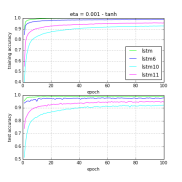
Figure 1: Training & Test accuracy, $\sigma=tanh,\eta=1\mathrm{e}{-3}$

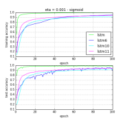
Figure 2: Training & Test accuracy, $\sigma=sigmoid,\eta=1\mathrm{e}{-3}$

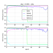
Figure 3: Training & Test accuracy, $\sigma=relu,\eta=1\mathrm{e}{-3}$

TABLE III: Best results obtained by $\eta=0.001$.

		$tanh$	$sigmoid$	$relu$
LSTM	train	1.000	0.9972	0.9829
	test	0.9909	0.9880	0.9843
LSTM6	train	0.9879	0.9495	0.9719
	test	0.9792	0.9513	0.9720
LSTM10	train	0.9273	0.9168	0.4018
	test	0.9225	0.9184	0.5226
LSTM11	train	0.9573	0.9407	0.9597
	test	0.9514	0.9403	0.9582

3.2 Searching for best $\eta$

We increased $\eta$ from $0.001$ to $0.005$ in increments of $0.001$. This led into an increase in test accuracy of model LSTM11 and model LSTM12, yielding values 95.31% and 93.56% respectively for the $tanh$ case. As expected, LSTM10 with the $relu$ activation failed progressively comparing to smaller $\eta$ values. The training and test accuracy of these new $\eta$ values are shown in Table IV and Table V.

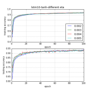
Figure 4: Training & Test accuracy of different $\eta$, lstm10, $tanh$

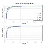
Figure 5: Training & Test accuracy of different $\eta$, lstm10, $sigmoid$

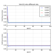
Figure 6: Training & Test accuracy of different $\eta$, lstm10, $relu$

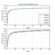
Figure 7: Training & Test accuracy of different $\eta$, lstm11, $tanh$

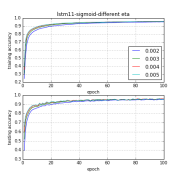
Figure 8: Training & Test accuracy of different $\eta$, lstm11, $sigmoid$

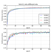
Figure 9: Training & Test accuracy of different $\eta$, lstm11, $relu$

TABLE IV: Best results obtained by LSTM10.

		$tanh$	$sigmoid$	$relu$
$\eta=0.002$	train	0.9376	0.9354	0.3319
	test	0.9366	0.9376	0.2510
$\eta=0.003$	train	0.9388	0.9389	0.1777
	test	0.9357	0.9367	0.0919
$\eta=0.004$	train	0.9348	0.9428	0.1946
	test	0.9350	0.9392	0.0954
$\eta=0.005$	train	0.9317	0.9453	0.1519
	test	0.9318	0.9444	0.0919

TABLE V: Best results obtained by LSTM11.

		$tanh$	$sigmoid$	$relu$
$\eta=0.002$	train	0.9566	0.9546	0.9602
	test	0.9511	0.9534	0.9583
$\eta=0.003$	train	0.9557	0.9601	0.9637
	test	0.9521	0.9598	0.9656
$\eta=0.004$	train	0.9552	0.9608	0.9607
	test	0.9531	0.9608	0.9582
$\eta=0.005$	train	0.9539	0.9611	0.9565
	test	0.9516	0.9635	0.9569

3.3 Finding $\eta$ for LSTM10 relu

We have explored a range of $\eta$ for LSTM10 with $relu$ activation to improve its performance. However, the effort was not successful. Increasing $\eta$ from $2e-6$ to $1e-5$ leads to an increase in accuracy with value of 53.13%. For $\eta$ less than $1\mathrm{e}{-5}$, the plots have increasing trend. However, after this point, the accuracy starts to drop after a number of epochs depending on the value of $\eta$.

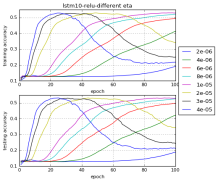
Figure 10: Training & Test accuracy of different $\eta$, lstm10, $relu$

4 Conclusion

In this study, we have described and evaluated two new reduced variants of LSTM model. We call these new models LSTM10 and LSTM11. These models have been examined and evaluated on the MNIST dataset with different activations and different learning rate $\eta$ values. In our part I and part II, we considered variants to the base LSTM by removing weights/biases from the gating equations only. In this study, we have reduced weights even within the main cell-memory equation of the model by converting a weight matrix to a vector and replace regular multiplication with (Hadamard) pointwise multiplication. The only difference between model LSTM10 and LSTM11 is that the latter retain the bias term in the gating equations. LSTM 6 is equivalent to the so-called basic recurrent neural network (bRNN), since all gating equation have been replaced by a fixed constant– see [8]. It has been found that all of variants, except model LSTM10 when using the activation $relu$, are comparable to a (standard) base LSTM RNN. We anticipate that further case studies and experiments would serve to fine-tune these findings.

References

- [1] Y. Bengio, P. Simard, and P. Frasconi. Learning long-term dependencies with gradient descent is difficult. IEE TRANSACTIONS ON NEURAL NETWORKS, 5, 1994.
- [2] N. Boulanger-Lewandowski, Y. Bengio, and P. Vincent. Modeling temporal dependencies in high-dimensional sequences: Application to polyphonic music generation and transcription, 2012.
- [3] F. Chollet. Keras github.
- [4] J. Chung, C. Gulcehre, K. Cho, and Y. Bengio. Empirical evaluation of gated recurrent neural networks on sequence modeling, 2014.
- [5] S. Hochreiter and J. Schmidhuber. Long short-term memory. Neural Computation, 9:1735–1780, 1997.
- [6] Q. V. Le, N. Jaitly, and H. G. E. A simple way to initialize recurrent networks of rectified linear units. 2015.
- [7] Y. Lu and F. Salem. Simplified gating in long short-term memory (lstm) recurrent neural networks. arXiv:1701.03441, 2017.
- [8] F. M. Salem. A basic recurrent neural network model. arXiv preprint arXiv:1612.09022, 2016.
- [9] F. M. Salem. Reduced parameterization of gated recurrent neural networks. MSU Memorandum, 7.11.2016.