Quantized-CP Approximation and Sparse Tensor Interpolation of Function Generated Data

Abstract

In this article we consider the iterative schemes to compute the canonical (CP) approximation of quantized data generated by a function discretized on a large uniform grid in an interval on the real line. This paper continues the research on the QTT method [16] developed for the tensor train (TT) approximation of the quantized images of function related data. In the QTT approach the target vector of length $2^{L}$ is reshaped to a $L^{th}$ order tensor with two entries in each mode (Quantized representation) and then approximated by the QTT tenor including $2r^{2}L$ parameters, where $r$ is the maximal TT rank. In what follows, we consider the Alternating Least-Squares (ALS) iterative scheme to compute the rank-$r$ CP approximation of the quantized vectors, which requires only $2rL\ll 2^{L}$ parameters for storage. In the earlier papers [17] such a representation was called Q_Can format, while in this paper we abbreviate it as the QCP representation. We test the ALS algorithm to calculate the QCP approximation on various functions, and in all cases we observed the exponential error decay in the QCP rank. The main idea for recovering a discretized function in the rank-$r$ QCP format using the reduced number the functional samples, calculated only at $O(2rL)$ grid points, is presented. The special version of ALS scheme for solving the arising minimization problem is described. This approach can be viewed as the sparse QCP-interpolation method that allows to recover all $2rL$ representation parameters of the rank-$r$ QCP tensor. Numerical examples show the efficiency of the QCP-ALS type iteration and indicate the exponential convergence rate in $r$.

AMS Subject classification: 15A69, 65F99.
Keywords: QTT tensor approximation, QCP data format, $L^{th}$ order tensors, canonical tensor approximation, CP rank, discretized function, uniform grid, Alternating Least Squares iteration.

1 Introduction

In many applications, the approximation or integration of functions inheriting the properties of $e^{-kx},\,e^{-kx^{2}},\,e^{-k|x|},\,\sin(kx)$ or $1/|x|^{\alpha}$ on an interval in $\mathbb{R}$ as well as functions depending on many parameters leads to the challenging numerical problems. Often a very fine grid is required to approximate sharp functions like the Gaussians $e^{-kx^{2}}$ for large values of $k$, highly oscillating functions or functions with multiple local singularities or cusps arising, for example, as the solution of PDEs discretized on fine spatial grid. The storage of the function values as well as simple arithmetic’s operations on data arising from sampling on large grids may easily become non-tractable. The additional difficulty arises if each function evaluation has very high cost, say, related to the solution of large linear system or spectral problem as well as to solving complicated PDE.

The quantics-TT (QTT) tensor approximation method, introduced and analyzed in [16] for some classes of discretized functions, is now a well established technique for data compression of long function generated vectors. It is based on the low-rank tensor approximation to the quantized image of a vector, where the tensor train (TT) format [31] was applied to the quantized multi-fold image. Based on the quantization (reshaping) of a long $2^{L}$-vector to a $L^{th}$-order tensor (Quantics) the consequent QTT tensor approximation has been proven to have low TT rank for a wide class of functional vectors. We refer to [30] where the TT approximation to the reshaped $2^{L}\times 2^{L}$ Laplacian type matrices was considered and analyzed numerically. The QTT tensor parametrization requires $O(2r^{2}L)$ storage size where $r$ is the upper bound on the TT rank parameters. Some examples on the successful application of the QTT tensor approximation to the solution of PDEs and in stochastic modeling can be found in [1, 5, 13, 14, 26] and in [19, 20, 22, 21, 23, 6, 25], among others.

The present paper continues the research on the QTT tensor approximation method [16] based on the use of TT format. In what follows we investigate the numerical schemes to compute canonical (CP) tensor approximation of the quantized tensor. This data format was introduced in [17] under the name Q_Can tensor representation. In this paper, we shall abbreviate the notion Q_Can as the QCP format. First, we briefly recall the main construction along the line of the QTT approximation. A given vector of size $N=2^{L}$ is reshaped (quantized) by successive dyadic folding to a $\underset{L}{\underbrace{2\times 2\times\ldots\times 2}}$ array. The rank $r$ representation of this tensor in the canonical format reduces the number of representation parameters from $2^{L}$ down to $2rL$, which is smaller than for the QTT format, characterized by the storage size $O(2r^{2}L)$. The following simple example shows why the QCP approximation of a vector does a job by reducing the number of representation parameters.

Let $f(x)=e^{-x}$ in $[0,1]$. Consider the nodes $0,h,2h,\ldots,15h$ on the interval $[0,1],$ where $h$ is the step size of the uniform grid. The function values at these discrete points form a vector ${\bf q}=[1,q,q^{2},\ldots,q^{15}]$ of length $N=2^{4}$, where $q=e^{-h}.$ Now reshape the vector ${\bf q}$ to obtain a $4$th order tensor ${\bf Q}\in\mathbb{R}^{2\times 2\times 2\times 2}$ that is the quantized image of ${\bf q}$. Following [16], we recall that the CP rank of this tensor is 1, and the corresponding explicit CP tensor representation reads as

$${\bf Q}=\left(\begin{array}[]{c}1\\ q\end{array}\right)\otimes\left(\begin{array}[]{c}1\\ q^{2}\end{array}\right)\otimes\left(\begin{array}[]{c}1\\ q^{4}\end{array}\right)\otimes\left(\begin{array}[]{c}1\\ q^{8}\end{array}\right).$$

One can see that the whole vector of size $N=2^{4}$ is represented only by 4 parameters, that means the logarithmic complexity scaling $\log_{2}N.$ In general, the CP rank of the quantized image of a vector of length $2^{L}$ generated by $f(x)=e^{-\lambda x}$ is $1$ and it is represented by only $\log_{2}2^{L}=L$ parameters, such that its explicit one-term representation is given by [16]

$${\bf Q}=\bigotimes_{p=1}^{L}\left(\begin{array}[]{c}1\\ q^{2^{p-1}}\end{array}\right).$$

We say that the CP rank of the quantized image of the discretized function $e^{-\lambda x}$ is $1.$ In general, the exact CP rank of rather simple functions like $e^{-x^{2}},\sin\,k\pi x,|x|^{\alpha},...$ etc. is not known. Construction and complexity analysis of ALS-type algorithms for computing the QCP approximation of quantized functions is the main aim of this article.

It is worth to note that the rank-$r$ QCP tensor is represented only by small number of parameters, $2Lr$, whereas the QTT format based on rank $r$ TT tensors is parametrized by $O(2Lr^{2})$ numbers as it was already mentioned. Based on this observation, we propose the QCP interpolation scheme using only small number of functional calls (of the order of $O(2Lr)$) which recovers the quantized tensor image. This concept leads to the promising enhancement of the QPC approximation of the complete $2^{L}$-vector because the small number of parameters in the arising minimization problem. For the practical implementation, we introduce the ALS type scheme to compute the sparse QCP interpolant.

In numerical examples, we test the ALS iterative scheme implementing the CP approximation on $15$th order tensors representing $2^{15}$-vectors generated by various functions. In all cases we observe the exponentially fast error decay in the QCP rank. Notice that the traditional ALS algorithm for CP tensors and its enhanced versions have been discussed in many articles [2, 3, 7, 8, 9, 12, 15, 22, 35, 36, 34]. Regularized ALS scheme was considered in [27, 28].

The efficient representation and multilinear algebra of large multidimensional vectors (tensors) can be based on their low-rank tensor approximation by using different tensor formats. We refer to reviews on the multilinear algebra [15, 11, 10, 29, 32] and to recent surveys on tensor numerical methods and their application in scientific computing [17, 18, 24, 4].

The rest of the paper is organized as follows. Some auxiliary technical results concerning the ALS-canonical algorithm are presented in section 2. Section 3 describes the particular QCP-ALS scheme which uses the complete information about the tensor. In section 4, we calculate the QCP approximation of some selected functions which appears in various applications. The main idea and basic ALS scheme for computing the QCP approximation by using the information on only few entries of the target vector is described in Section 5, where the numerical illustrations are also presented. The approximation by using incomplete data can be viewed as the sparse QCP interpolation of function generated vectors. Some useful notations, definitions and a simple example of the scheme for QCP approximation of a $4^{th}$ order tensor are given in Appendix.

In this article, we often use MATLAB notations, for example ${\bf X}=\mbox{reshape}({\bf x},2,...,2)$. The Frobenius norm of a tensor ${\bf X}=[x_{i_{1}i_{2}\ldots i_{d}}]\in\mathbb{R}^{n_{1}\times n_{2}\times\ldots\times n_{d}}$ is defined as the square root of the sum of squares of all its elements $x_{i_{1}i_{2}\ldots i_{d}}$, i.e,

$$\left\|{\bf X}\right\|_{F}=\sqrt{\sum_{i_{1}=1}^{n_{1}}\sum_{i_{2}=1}^{n_{2}}\ldots\sum_{i_{d}=1}^{n_{d}}x_{i_{1}i_{2}\ldots i_{d}}^{2}}.$$

2 Technical results for ALS

For convenience and better understanding of our notation and some technical results in the upcoming sections, we provide the proofs of some basic results (see [36]), which are useful in the construction of ALS algorithm, and give some simple examples of ALS iteration for canonical approximation of a tensor.

A complete description of each iteration step of ALS for a fourth order tensor $\chi$ is given in the appendix A3. In the steps 1, 2, 3 and 4 of A3, we need to obtain products like $(C\odot B\odot A)^{T}(C\odot B\odot A)$ and $(C\odot B\odot A)^{T}\chi(:,:,:,1)$, where $\odot$ is the Khatri-Rao product of matrices defined in appendix A2. An efficient way of obtaining these products is described below. First, we show it for products which appear in the canonical approximation of a third order tensor and then generalize it for $d^{th}$ order tensors.

2.1 Fast evaluation of $\left(B\odot C\right)^{T}\left(B\odot C\right)$

In the Alternating Least Squares method, to get the Canonical approximation to a third order tensor, we need to compute $\left(B\odot C\right)^{T}\left(B\odot C\right).$ This usually requires $O(r^{2}n_{1}n_{2})+n_{1}n_{2}r$ arithmetic operations. Now we show the efficient way to compute it.

Lemma 1. If $B=[\mathbf{b}_{1}|\mathbf{b}_{2}|\ldots|\mathbf{b}_{r}]\in\mathbb{R}^{n_{1}\times r}$ and $C=[\mathbf{c}_{1}|\mathbf{c}_{2}|\ldots|\mathbf{c}_{r}]\in\mathbb{R}^{n_{2}\times r},$ then $\displaystyle\left(B\odot C\right)^{T}\left(B\odot C\right)=\left(B^{T}B\right)\circ\left(C^{T}C\right)$ where $\circ$ denotes the Hadamard product of matrices.

Proof: As defined in appendix A2,

$$B\odot C=[\mathbf{b}_{1}\otimes\mathbf{c}_{1}|\mathbf{b}_{2}\otimes\mathbf{c}_{2}|\ldots|\mathbf{b}_{r}\otimes\mathbf{c}_{r}]\in\mathbb{R}^{n_{1}n_{2}\times r}.$$

So

$$(B\odot C)^{T}(B\odot C)=\left[\begin{array}[]{c}(\mathbf{b}_{1}\otimes\mathbf{c}_{1})^{T}\\ (\mathbf{b}_{2}\otimes\mathbf{c}_{2})^{T}\\ \vdots\\ (\mathbf{b}_{r}\otimes\mathbf{c}_{r})^{T}\end{array}\right]_{r\times n_{1}n_{2}}[\mathbf{b}_{1}\otimes\mathbf{c}_{1}|\mathbf{b}_{2}\otimes\mathbf{c}_{2}|\ldots|\mathbf{b}_{r}\otimes\mathbf{c}_{r}]_{n_{1}n_{2}\times r}$$

$$=\left[\begin{array}[]{ccccc}(\mathbf{b}_{1}\otimes\mathbf{c}_{1})^{T}(\mathbf{b}_{1}\otimes\mathbf{c}_{1})&(\mathbf{b}_{1}\otimes\mathbf{c}_{1})^{T}(\mathbf{b}_{2}\otimes\mathbf{c}_{2})&...&...&(\mathbf{b}_{1}\otimes\mathbf{c}_{1})^{T}(\mathbf{b}_{r}\otimes\mathbf{c}_{r})\\ (\mathbf{b}_{2}\otimes\mathbf{c}_{2})^{T}(\mathbf{b}_{1}\otimes\mathbf{c}_{1})&(\mathbf{b}_{2}\otimes\mathbf{c}_{2})^{T}(\mathbf{b}_{2}\otimes\mathbf{c}_{2})&...&...&(\mathbf{b}_{2}\otimes\mathbf{c}_{2})^{T}(\mathbf{b}_{r}\otimes\mathbf{c}_{r})\\ \vdots&\vdots&&&\vdots\\ (\mathbf{b}_{r}\otimes\mathbf{c}_{r})^{T}(\mathbf{b}_{1}\otimes\mathbf{c}_{1})&(\mathbf{b}_{r}\otimes\mathbf{c}_{r})^{T}(\mathbf{b}_{2}\otimes\mathbf{c}_{2})&...&...&(\mathbf{b}_{r}\otimes\mathbf{c}_{r})^{T}(\mathbf{b}_{r}\otimes\mathbf{c}_{r})\end{array}\right]$$

$$=\left[\begin{array}[]{ccccc}(\mathbf{b}_{1}^{T}\otimes\mathbf{c}_{1}^{T})(\mathbf{b}_{1}\otimes\mathbf{c}_{1})&(\mathbf{b}_{1}^{T}\otimes\mathbf{c}_{1}^{T})(\mathbf{b}_{2}\otimes\mathbf{c}_{2})&...&...&(\mathbf{b}_{1}^{T}\otimes\mathbf{c}_{1}^{T})(\mathbf{b}_{r}\otimes\mathbf{c}_{r})\\ (\mathbf{b}_{2}^{T}\otimes\mathbf{c}_{2}^{T})(\mathbf{b}_{1}\otimes\mathbf{c}_{1})&(\mathbf{b}_{2}^{T}\otimes\mathbf{c}_{2}^{T})(\mathbf{b}_{2}\otimes\mathbf{c}_{2})&...&...&(\mathbf{b}_{2}^{T}\otimes\mathbf{c}_{2}^{T})(\mathbf{b}_{r}\otimes\mathbf{c}_{r})\\ \vdots&\vdots&&&\vdots\\ (\mathbf{b}_{r}^{T}\otimes\mathbf{c}_{r}^{T})(\mathbf{b}_{1}\otimes\mathbf{c}_{1})&(\mathbf{b}_{r}^{T}\otimes\mathbf{c}_{r}^{T})(\mathbf{b}_{2}\otimes\mathbf{c}_{2})&...&...&(\mathbf{b}_{r}^{T}\otimes\mathbf{c}_{r}^{T})(\mathbf{b}_{r}\otimes\mathbf{c}_{r})\end{array}\right]\,\,\,\,$$ (see  P1  in  A1)

$$=\left[\begin{array}[]{ccccc}(\mathbf{b}_{1}^{T}\mathbf{b}_{1}\otimes\mathbf{c}_{1}^{T}\mathbf{c}_{1})&(\mathbf{b}_{1}^{T}\mathbf{b}_{2}\otimes\mathbf{c}_{1}^{T}\mathbf{c}_{2})&...&...&(\mathbf{b}_{1}^{T}\mathbf{b}_{r}\otimes\mathbf{c}_{1}^{T}\mathbf{c}_{r})\\ (\mathbf{b}_{2}^{T}\mathbf{b}_{1}\otimes\mathbf{c}_{2}^{T}\mathbf{c}_{1})&(\mathbf{b}_{2}^{T}\mathbf{b}_{2}\otimes\mathbf{c}_{2}^{T}\mathbf{c}_{2})&...&...&(\mathbf{b}_{2}^{T}\mathbf{b}_{r}\otimes\mathbf{c}_{2}^{T}\mathbf{c}_{r})\\ \vdots&\vdots&&&\vdots\\ (\mathbf{b}_{r}^{T}\mathbf{b}_{1}\otimes\mathbf{c}_{r}^{T}\mathbf{c}_{1})&(\mathbf{b}_{r}^{T}\mathbf{b}_{2}\otimes\mathbf{c}_{r}^{T}\mathbf{c}_{2})&...&...&(\mathbf{b}_{r}^{T}\mathbf{b}_{r}\otimes\mathbf{c}_{r}^{T}\mathbf{c}_{r})\end{array}\right].\,\,\,\,\,\,\,\,\,\,\,\,\,\,\,\,\,\,\,\,\,\,\,\,\,\,\,\,\,\,\,\,\,\,\,\,\,\,$$ (see  P3  in  A1)

Since $\mathbf{b}_{i}^{T}\mathbf{b}_{j}$ and $\mathbf{c}_{i}^{T}\mathbf{c}_{j}$ are scalars, $(\mathbf{b}_{i}^{T}\mathbf{b}_{j})\otimes(\mathbf{c}_{i}^{T}\mathbf{c}_{j})=(\mathbf{b}_{i}^{T}\mathbf{b}_{j})\cdot(\mathbf{c}_{i}^{T}\mathbf{c}_{j})$. Therefore,

$$(B\odot C)^{T}(B\odot C)=\left[\begin{array}[]{cccc}\mathbf{b}_{1}^{T}\mathbf{b}_{1}&\mathbf{b}_{1}^{T}\mathbf{b}_{2}&...&\mathbf{b}_{1}^{T}\mathbf{b}_{r}\\ \mathbf{b}_{2}^{T}\mathbf{b}_{1}&\mathbf{b}_{2}^{T}\mathbf{b}_{2}&...&\mathbf{b}_{2}^{T}\mathbf{b}_{r}\\ \\ \mathbf{b}_{r}^{T}\mathbf{b}_{1}&\mathbf{b}_{r}^{T}\mathbf{b}_{2}&...&\mathbf{b}_{r}^{T}\mathbf{b}_{r}\end{array}\right]\circ\left[\begin{array}[]{cccc}\mathbf{c}_{1}^{T}\mathbf{c}_{1}&\mathbf{c}_{1}^{T}\mathbf{c}_{2}&...&\mathbf{c}_{1}^{T}\mathbf{c}_{r}\\ \mathbf{c}_{2}^{T}\mathbf{c}_{1}&\mathbf{c}_{2}^{T}\mathbf{c}_{2}&...&\mathbf{c}_{2}^{T}\mathbf{c}_{r}\\ \\ \mathbf{c}_{r}^{T}\mathbf{c}_{1}&\mathbf{c}_{r}^{T}\mathbf{c}_{2}&...&\mathbf{c}_{r}^{T}\mathbf{c}_{r}\end{array}\right]=(B^{T}B)\circ(C^{T}C).\,\,\,\,\,\,\,\,$$

So one can easily show that $B^{T}B$ requires $O(n_{1}r^{2})$ and $C^{T}C$ requires $O(n_{2}r^{2})$ arithmetic operations. Therefore, the computational complexity to compute $(B\odot C)^{T}(B\odot C)$ is $O((n_{1}+n_{2})r^{2})+r^{2}.$

Generalization of Lemma 1

Here we generalize Lemma 1 to more than two matrices. Let us consider $A_{1},A_{2},\ldots,A_{L}$ to be matrices of the same size $n\times r.$ Then by recursion one can easily prove that

$$\left[A_{L}\odot..\odot A_{i+1}\odot A_{i-1}\odot A_{i-2}\odot..\odot A_{1}\right]^{T}\left[A_{L}\odot..\odot A_{i+1}\odot A_{i-1}\odot A_{i-2}\odot..\odot A_{1}\right]\,\,\,\,\,\,\,\,\,\,\,\,\,\,\,\,\,\,\,\,\,\,\,\,\,\,\,\,\,\,\,\,\,\,\,\,$$

$$=\left[\left(A_{L}\odot..\odot A_{i+1}\odot A_{i-1}\odot A_{i-2}\odot..\odot A_{2}\right)\odot A_{1}\right]^{T}\left[\left(A_{L}\odot..\odot A_{i+1}\odot A_{i-1}\odot A_{i-2}\odot..\odot A_{2}\right)\odot A_{1}\right]$$

$$=\left(A_{L}\odot..\odot A_{i+1}\odot A_{i-1}\odot A_{i-2}\odot..\odot A_{2}\right)^{T}\left(A_{L}\odot..\odot A_{i+1}\odot A_{i-1}\odot A_{i-2}\odot..\odot A_{2}\right)\circ A_{1}^{T}A_{1}\,\,\,\,\,\,\,\,\,\,\,\,\,$$

$$\vdots\,\,\,\,\,\,\,\,\,\,\,\,\,\,\,\,\,\,\,\,\,\,\,\,\,\,\,\,\,\,\,\,\,\,\,\,\,\,\,\,\,\,\,\,\,\,\,\,\,\,\,\,\,\,\,\,\,\,\,\,\,\,\,\,\,\,\,\,\,\,\,\,\,\,\,\,\,\,\,\,\,\,\,\,\,\,\,$$

$$=\left(A_{L}^{T}A_{L}\right)\circ\left(A_{L-1}^{T}A_{L-1}\right)\circ\ldots\circ\left(A_{i+1}^{T}A_{i+1}\right)\circ\left(A_{i-1}^{T}A_{i-1}\right)\circ\ldots\circ\left(A_{2}^{T}A_{2}\right)\circ\left(A_{1}^{T}A_{1}\right).\,\,\,\,\,\,\,\,\,\,\,\,\,\,\,\,\,\,\,\,\,\,\,\,$$

The computational complexity to compute the above is $O((L-1)nr^{2})$ whereas the direct computation of this product requires $n^{L-1}r+O(r^{2}n^{L-1}).$ So this is much faster.

2.2 Fast evaluation of $\left(B\odot C\right)^{T}\,\mathbf{x}$

In ALS, we also need to compute $\left(B\odot C\right)^{T}\mathbf{x}$ for $\mathbf{x}\in\mathbb{R}^{n_{1}n_{2}}.$ It would require $3n_{1}n_{2}r-r$ arithmetic operations including $n_{1}n_{2}r$ operations for computing $\left(B\odot C\right).$ This complexity can be further improved in the following way.

Lemma 2: If $B=[\mathbf{b}_{1}|\mathbf{b}_{2}|\ldots|\mathbf{b}_{r}]\in\mathbb{R}^{n_{1}\times r}$ and $C=[\mathbf{c}_{1}|\mathbf{c}_{2}|\ldots|\mathbf{c}_{r}]\in\mathbb{R}^{n_{2}\times r}$ and $\mathbf{x}\in\mathbb{R}^{n_{1}n_{2}}$ then

$$\mathbf{y}=\left(B\odot C\right)^{T}\,\mathbf{x}=\left[\begin{array}[]{c}\mathbf{c}_{1}^{T}X\mathbf{b}_{1}\\ \mathbf{c}_{2}^{T}X\mathbf{b}_{2}\\ \vdots\\ \mathbf{c}_{r}^{T}X\mathbf{b}_{r}\end{array}\right].$$

Where $X=\textrm{reshape}(\mathbf{x},n_{2},n_{1}).$
Proof: Let $\mathbf{x}=[x_{1},x_{2},\ldots,x_{n_{1}n_{2}}]^{T}.$ Reshape the vector $\mathbf{x}$ as an $n_{2}\times n_{1}$ matrix $X$

$$X=\left[\begin{array}[]{cccc}x_{1}&x_{n_{2}+1}&...&x_{(n_{1}-1)n_{2}+1}\\ x_{2}&x_{n_{2}+2}&&x_{(n_{1}-1)n_{2}+2}\\ \vdots&\vdots\\ x_{n_{2}}&x_{2n_{2}}&&x_{n_{1}n_{2}}\end{array}\right].$$

$(B\odot C)^{T}\mathbf{x}$ is given by

$$(B\odot C)^{T}\mathbf{x}=[\mathbf{b}_{1}\otimes\mathbf{c}_{1}|\mathbf{b}_{2}\otimes\mathbf{c}_{2}|\ldots|\mathbf{b}_{r}\otimes\mathbf{c}_{r}]_{n_{1}n_{2}\times r}^{T}\,\mathbf{x}_{n_{1}n_{2}\times 1}$$

$$=\left[\begin{array}[]{c}(\mathbf{b}_{1}\otimes\mathbf{c}_{1})^{T}\\ (\mathbf{b}_{2}\otimes\mathbf{c}_{2})^{T}\\ \vdots\\ (\mathbf{b}_{r}\otimes\mathbf{c}_{r})^{T}\end{array}\right]_{r\times n_{1}n_{2}}\mathbf{x}_{n_{1}n_{2}\times 1}=\left[\begin{array}[]{c}(\mathbf{b}_{1}\otimes\mathbf{c}_{1})^{T}\mathbf{x}\\ (\mathbf{b}_{2}\otimes\mathbf{c}_{2})^{T}\mathbf{x}\\ \vdots\\ (\mathbf{b}_{r}\otimes\mathbf{c}_{r})^{T}\mathbf{x}\end{array}\right]\,\,=\,\left[\begin{array}[]{c}\mathbf{c}_{1}^{T}X\mathbf{b}_{1}\\ \mathbf{c}_{2}^{T}X\mathbf{b}_{2}\\ \vdots\\ \mathbf{c}_{r}^{T}X\mathbf{b}_{r}\end{array}\right].$$

Where $X=\textrm{reshape}(\mathbf{x},n_{2},n_{1}).$ In the last step of the above equation we have used $(\mathbf{b}_{i}^{T}\otimes\mathbf{c}_{i}^{T})\mathbf{x}=\mathbf{c}_{i}^{T}X\mathbf{b}_{i}.$ This can be shown easily in the following way.

Let $\mathbf{b}_{i}=[b_{1i},b_{2i},\ldots,b_{n_{1}i}]^{T}$ and $\mathbf{c}_{i}=[c_{1i},c_{2i},\ldots,c_{n_{2}i}]^{T}.$ Then

$$(\mathbf{b}_{i}\otimes\mathbf{c}_{i})^{T}\mathbf{x} = \left[\begin{array}[]{c}b_{1i}c_{1i}\\ b_{1i}c_{2i}\\ \vdots\\ b_{1i}c_{n_{2}i}\\ b_{2i}c_{1i}\\ \vdots\\ b_{n_{1}i}c_{n_{2}i}\end{array}\right]^{T}\left[\begin{array}[]{c}x_{1}\\ x_{2}\\ \vdots\\ x_{n_{2}}\\ x_{n_{2}+1}\\ \vdots\\ x_{n_{2}n_{1}}\end{array}\right]\,\,\,\,\,\,\,\,\,\,\,\,\,\,\,\,\,\,\,\,\,\,\,\,\,\,\,\,\,\,\,\,\,$$

$$= b_{1i}c_{1i}x_{1}+b_{1i}c_{2i}x_{2}+........+b_{1i}c_{n_{2}i}x_{n_{2}}$$

$$+ b_{2i}c_{1i}x_{n_{2}+1}+...................+b_{2i}c_{n_{2}i}x_{2n_{2}}$$

$$\vdots$$

$$+ b_{n_{1}i}c_{1i}x_{n_{2}(n_{1}-1)+1}+........+b_{n_{1}i}c_{n_{2}i}x_{n_{1}n_{2}}$$

$$= c_{1i}\left(b_{1i}x_{1}+b_{2i}x_{n_{2}+1}+.....+b_{n_{1}i}x_{n_{2}(n_{1}-1)+1}\right)\,\,\,\,\,\,\,\,\,\,\,\,\,\,\,\,\,\,\,\,\,\,\,\,\,\,\,\,\,\,\,\,\,\,\,\,\,\,\,$$

$$+ c_{2i}\left(b_{1i}x_{2}+b_{2i}x_{n_{2}+2}+.....+b_{n_{1}i}x_{n_{2}(n_{1}-1)+2}\right)\,\,\,\,\,\,\,\,\,\,\,\,\,\,\,\,\,\,\,\,\,\,\,\,\,\,\,\,\,\,\,\,\,\,\,\,\,\,\,$$

$$\vdots$$

$$+ c_{n_{2}i}\left(b_{1i}x_{n_{2}}+b_{2i}x_{2n_{2}}+..............+b_{n_{1}i}x_{n_{2}n_{1}}\right)\,\,\,\,\,\,\,\,\,\,\,\,\,\,\,\,\,\,\,\,\,\,\,\,\,\,\,\,\,\,\,\,\,\,\,\,\,\,\,$$

$$= [c_{1i},c_{2i},...,c_{n_{2}i}]\left[\begin{array}[]{c}b_{1i}x_{1}+b_{2i}x_{n_{2}+1}+.....+b_{n_{1}i}x_{n_{2}(n_{1}-1)+1}\\ b_{1i}x_{2}+b_{2i}x_{n_{2}+2}+.....+b_{n_{1}i}x_{n_{2}(n_{1}-1)+2}\\ \vdots\\ b_{1i}x_{n_{2}}+b_{2i}x_{2n_{2}}+..............+b_{n_{1}i}x_{n_{2}n_{1}}\end{array}\right]$$

$$= [c_{1i},c_{2i},...,c_{n_{2}i}]\left[\begin{array}[]{cccc}x_{1}&x_{n_{2}+1}&....&x_{(n_{1}-1)n_{2}+1}\\ x_{2}&x_{n_{2}+2}&....&x_{(n_{1}-1)n_{2}+2}\\ \vdots&\vdots&\vdots\\ x_{n_{2}}&x_{2n_{2}}&.....&x_{n_{1}n_{2}}\end{array}\right]\left[\begin{array}[]{c}b_{1i}\\ b_{2i}\\ \vdots\\ b_{n_{1}i}\end{array}\right]\,\,\,\,\,\,$$

$$= \mathbf{c}_{i}^{T}X\mathbf{b}_{i}\,\,\,.$$

Here $n_{2}(2n_{1}-1)$ operations are required to compute $X_{n_{2}n_{1}}\mathbf{b}_{i}$ and $(2n_{2}-1)$ operations to compute $\mathbf{c}_{i}^{T}(X_{n_{2}n_{1}}\mathbf{b}_{i}).$ Therefore the overall computational complexity is $2n_{1}n_{2}r+n_{2}r-r$ which is less than the complexity for computing $(B\odot C)^{T}\mathbf{x}$ directly.

2.2.1 Generalization of Lemma 2

Let us look at Lemma 2 in the case of three matrices $A_{4}\in\mathbb{R}^{n_{4}\times r},\,A_{3}\in\mathbb{R}^{n_{3}\times r}$ and $A_{2}\in\mathbb{R}^{n_{2}\times r}.$ Let $\mathbf{x}\in\mathbb{R}^{n_{4}n_{3}n_{2}}.$ We look at $(A_{4}\odot A_{3}\odot A_{2})^{T}\mathbf{x}.$ Reshape the vector $\mathbf{x}$ into a matrix of size $n_{2}n_{3}\times n_{4}.$ Let $X_{4}=reshape(\mathbf{x},n_{2}n_{3},n_{4}).$ Then

$$(A_{4}\odot A_{3}\odot A_{2})^{T}\mathbf{x}=\left[\begin{array}[]{c}(A_{3}\odot A_{2})_{1}^{T}X_{4}(A_{4})_{1}\\ (A_{3}\odot A_{2})_{2}^{T}X_{4}(A_{4})_{2}\\ \vdots\\ (A_{3}\odot A_{2})_{r}^{T}X_{4}(A_{4})_{r}\end{array}\right].$$

Here $(A_{4})_{i}$ is the $i^{th}$ column of $A_{4}$ with size $n_{4}\times 1.$ So the size of $X_{4}(A_{4})_{i}$ is $n_{2}n_{3}\times 1.$ Let us denote the vector $X_{4}(A_{4})_{i}$ by

$$(\mathbf{x}_{4})_{i}=X_{4}(A_{4})_{i},\,\,i=1,2,\ldots,r.$$

Now reshape each $(\mathbf{x}_{4})_{i}$, $i=1,2,\ldots,r$ into matrices $(X_{3})_{i}\in\mathbb{R}^{n_{2}\times n_{3}}.$ Then

$$(A_{4}\odot A_{3}\odot A_{2})^{T}\mathbf{x}=\left[\begin{array}[]{c}(A_{3}\odot A_{2})_{1}^{T}(\mathbf{x}_{4})_{1}\\ (A_{3}\odot A_{2})_{2}^{T}(\mathbf{x}_{4})_{2}\\ \vdots\\ (A_{3}\odot A_{2})_{r}^{T}(\mathbf{x}_{4})_{r}\end{array}\right]=\left[\begin{array}[]{c}(A_{2})_{1}^{T}(X_{3})_{1}(A_{3})_{1}\\ (A_{2})_{2}^{T}(X_{3})_{2}(A_{3})_{2}\\ \vdots\\ (A_{2})_{r}^{T}(X_{3})_{r}(A_{3})_{r}\end{array}\right].$$

Computational complexity

The computational complexity of the general product $(A_{L}\odot A_{L-1}\odot\ldots\odot A_{2})^{T}\mathbf{x}$ by the above technique is $r(2n-1)\left(\frac{n^{L-1}-1}{n-1}\right)$, where $A_{i}\in\mathbb{R}^{n\times r}$ and ${\mathbf{x}\in\mathbb{R}^{n^{L-1}}}$, whereas the direct computation of this product is a bit more expensive, it requires $n^{L-1}r+O(rn^{L-1})$ arithmetic operations including the computation of $A_{L}\odot A_{L-1}\odot\ldots\odot A_{2}$.

3 QCP Algorithm

Let $f$ be a function discretized on a fine grid of size $2^{L}\,(\textrm{for example}\,L=15)$ with uniform length in an interval. The function values at the grid points generate a vector of size $2^{L}.$ As described in the introduction we can reshape this long vector as a tensor of order $L$ and one can approximate it as a sum of products of vectors of length $2$. Fig. 1 shows an example of a ($3^{rd}$order tensor) quantized vector of length $2^{3},$ $[\tau_{1},\tau_{2},\tau_{3},\ldots,\tau_{8}]^{T}.$ The construction of a rank $r$ canonical approximation of such a tensor using Alternative Least Squares method is described below.

Figure 1: $3^{rd}$ order tensor.

Let $I=[a,b].$ Consider an uniform mesh with mesh size $h=\frac{1}{2^{L}-1}.$ Let $\mathbf{f}$ be the vector of length $2^{L}$ whose entries are the values of the given function $f$ at these $2^{L}$ points on the grid. Let us denote $\mathbf{f}$ by

$$\mathbf{f}=[\tau_{1},\tau_{2},\tau_{3},\ldots,\tau_{2^{L}}]^{T}.$$ (16)

Let $\chi$ be the quantized $L^{th}$ order tensor, given by

$$\chi=reshape(\mathbf{f},\underset{L}{\underbrace{2,2,\ldots,2}})\in\mathbb{R}^{2\times 2\times...\times 2}.$$

The precise definition of this operation is shortly recalled here:

The vector $\mathbf{f}$ is reshaped to its quantics image in ${\displaystyle{\displaystyle\otimes_{J=1}^{L}}}\mathbb{R}^{2}$ by dyadic folding,

$$\mathcal{G}_{2,L}:\,\mathbf{f}\rightarrow\chi=\chi(\mathbf{j})\in\otimes_{J=1}^{L}\mathbb{R}^{2},\,\mathbf{j}=\{j_{1},j_{2},\ldots,j_{L}\},\quad\text{with}\quad j_{\upsilon}\in\{1,2\},\upsilon=1,2,\ldots,L,$$

where for fixed $i,$ we have $\chi(\mathbf{j}):=\mathbf{f}(i)$ and $j_{\upsilon}=j_{\upsilon}(i)$ is defined via $2-$coding, $j_{\upsilon}-1=C_{-1+\upsilon},$ such that the coefficients $C_{-1+\upsilon}$ are found from the dyadic representation of $i-1,$

$$i-1=C_{0}+C_{1}\,2+C_{2}\,2^{2}+\ldots+C_{L-1}\,2^{L-1}\equiv{\displaystyle\sum_{\upsilon=1}^{L}(j_{\upsilon}-1)\,2^{\upsilon-1}.}$$

The rank $r$ canonical approximation of the $L^{th}$ order tensor is

$$\chi\cong\sum_{k=1}^{r}\mathbf{a}_{k}^{(1)}\otimes\mathbf{a}_{k}^{(2)}\otimes\ldots\otimes\mathbf{a}_{k}^{(L)}$$ (17)

where each $\mathbf{a}_{k}^{(i)}=\left[\begin{array}[]{c}a_{1,k}^{(i)}\\ a_{2,k}^{(i)}\end{array}\right]$ is a $2\times 1$ vector and $\otimes$ is the usual tensor product.

Let

$$A_{1}=[\mathbf{a}_{1}^{(1)},\mathbf{a}_{2}^{(1)},\ldots,\mathbf{a}_{r}^{(1)}],A_{2}=[\mathbf{a}_{1}^{(2)},\mathbf{a}_{2}^{(2)},\ldots,\mathbf{a}_{r}^{(2)}],\ldots,A_{L}=[\mathbf{a}_{1}^{(L)},\mathbf{a}_{2}^{(L)},\ldots,\mathbf{a}_{r}^{(L)}].$$

Here $A_{1},A_{2},\ldots,A_{L}$ are $2\times r$ matrices, corresponding to $L$ different directions, whose columns are the unknown vectors in equation (2).

The formulation of the ALS is the following:

$$\textrm{Minimize}\,\,\,\frac{1}{2}\left\|\chi-\sum_{k=1}^{r}\mathbf{a}_{k}^{(1)}\otimes\mathbf{a}_{k}^{(2)}\otimes\ldots\otimes\mathbf{a}_{k}^{(L)}\right\|_{F}^{2},$$ (18)

where $\left\|.\right\|_{F}$ is the Frobenius norm of a tensor.

In the ALS approach, this functional is minimized in an alternating way. ALS fixes all $A_{j},\,j\neq i,j=1,2,\ldots,L$ to minimize for $A_{i}$ and continue this process until some convergence criterion is satisfied. That is, first fix $A_{2},A_{3},\ldots,A_{L}$ to solve for $A_{1}$ and then fix $A_{1},A_{3},\ldots,A_{L}$ to solve for $A_{2}$ and so on and then fixes $A_{1},A_{2},\ldots,A_{L-1}$ to solve for $A_{L}$ and continue the process.

At each iteration of the ALS approach, we have $L$ steps. First, we start with an initial guess on $A_{2},A_{3},\ldots,A_{L}$ and solve for $A_{1}$, this gives the initial guess for the next step. Since we are fixing $L-1$ matrices and solving for one of the matrices $A_{i},\,i=1,2,\ldots,L$ at each step of an iteration, the problem is reduced to a linear least-squares problem.
In the $i^{th}$ step of an iteration, we fix $A_{1},A_{2},\ldots,A_{i-1},A_{i+1},\ldots,A_{L}$ and solve for
$A_{i}=\left[\begin{array}[]{cccc}a_{1,1}^{(i)}&a_{1,2}^{(i)}&...&a_{1,r}^{(i)}\\ a_{2,1}^{(i)}&a_{2,2}^{(i)}&...&a_{2,r}^{(i)}\end{array}\right].$ The resulting linear least-squares problem is:

$$\textrm{{minimize}}\,\,\mathcal{F},\,\,\,\,\,\,\,\,\,\,\,\,\,\,\,\,\,\,\,\,\,\,\,\,\,\,\,\,\,\,\,\,\,\,\,\,\,\,\,\,\,\,\,\,\,\,\,\,\,\,\,\,\,\,\,\,\,\,\,\,\,\,\,\,\,\,\,\,\,\,\,\,\,\,\,\,\,\,\,\,\,\,\,\,\,\,\,\,\,\,\,\,\,\,\,\,\,\,\,\,\,$$

$$\textrm{where}\,\,\mathcal{F}=\frac{1}{2}\left\|\chi-\sum_{k=1}^{r}\mathbf{a}_{k}^{(1)}\otimes\mathbf{a}_{k}^{(2)}\otimes\ldots\otimes\mathbf{a}_{k}^{(L)}\right\|_{F}^{2}\,\,\textrm{with}\,\,A_{1},A_{2},\ldots,A_{i-1},A_{i+1},\ldots,A_{L}\,\,\textrm{fixed}.$$ (19)

This gives the equations

$$\frac{\partial\mathcal{F}}{\partial a_{1,1}^{(i)}}=\frac{\partial\mathcal{F}}{\partial a_{1,2}^{(i)}}=\ldots=\frac{\partial\mathcal{F}}{\partial a_{1,r}^{(i)}}=0\quad\textrm{and}\quad\frac{\partial\mathcal{F}}{\partial a_{2,1}^{(i)}}=\frac{\partial\mathcal{F}}{\partial a_{2,2}^{(i)}}=\ldots=\frac{\partial\mathcal{F}}{\partial a_{2,r}^{(i)}}=0.$$

These equations can be written in the form

$$\left[\begin{array}[]{cc}\hat{A}_{i}^{T}\hat{A}_{i}\\ &\hat{A}_{i}^{T}\hat{A}_{i}\end{array}\right]\left[\begin{array}[]{c}\left[\begin{array}[]{c}a_{1,1}^{(i)}\\ a_{1,2}^{(i)}\\ \vdots\\ a_{1,r}^{(i)}\end{array}\right]\\ \begin{array}[]{c}\left[\begin{array}[]{c}a_{2,1}^{(i)}\\ a_{2,2}^{(i)}\\ \vdots\\ a_{2,r}^{(i)}\end{array}\right]\end{array}\end{array}\right]=\left[\begin{array}[]{c}\hat{A}_{i}^{T}\chi(:,\ldots,:,1,:,\ldots,:)\\ \hat{A}_{i}^{T}\chi(:,\ldots,:,2,:,\ldots,:)\end{array}\right].$$ (35)

Here $\hat{A}_{i}=A_{L}\odot A_{L-1}\odot...\odot A_{i+1}\odot A_{i-1}\odot...\odot A_{1},$ where $\odot$ denotes the Khatri-Rao product of matrices (see A2). This $\hat{A}_{i}$ is a $2^{L-1}\times r$ matrix and $\chi(:,\ldots,:,j,:,\ldots,:)$  $j=1,2$ is a vector of length $2^{L-1}.$ $\hat{A}_{i}^{T}\hat{A}_{i}$ is a $r\times r$ symmetric positive definite matrix. The direct computation of $\hat{A}_{i}^{T}\hat{A}_{i}$ and $\hat{A}_{i}^{T}\chi(:,\ldots,:,j,:,\ldots,:)$ is expensive. The fast computation of these products are described in section 2.
Remark: For a better understanding of the structure of $\hat{A}_{i}$ and the derivation of (5) we refer to appendix A3. All steps of the ALS algorithm for rank-2 canonical approximation of a $4^{th}$ order tensor are shown there in detail.

>From equation (5) one can see that we need to solve two $r\times r$ linear systems with the same matrix $\hat{A}_{i}^{T}\hat{A}_{i}$ and different right hand side vectors at each step of an iteration. We continue the iterations until a convergence criterion is reached.

Algorithm

—————————————————————————————————————————

Define tolerance $\epsilon$

Maximum iterations=Maxiter

Initialize $A_{i}\in\mathbb{R}^{2\times r},i=1,2,\ldots,L.$

while iter<=Maxiter

$C_{i}=A_{i},i=1,2,\ldots,L$

for $i=1,2,..L$

Obtain $\hat{A}_{i}=A_{L}\odot A_{L-1}\odot\ldots\odot A_{i+1}\odot A_{i-1}\odot\ldots\odot A_{1}$; $\hat{A}_{i}^{T}\chi(:,\ldots,:,j,:,\ldots,:)$ for $j=1,2$

Solve $\hat{A}_{i}^{T}\hat{A}_{i}$$\left[\begin{array}[]{c}a_{1,1}^{(i)}\\ a_{1,2}^{(i)}\\ \vdots\\ a_{1,r}^{(i)}\end{array}\right]=\hat{A}_{i}^{T}\chi(:,\ldots,:,1,:,\ldots,:)\,\,\textrm{and analog}\,\,\,\hat{A}_{i}^{T}\hat{A}_{i}\begin{array}[]{c}\left[\begin{array}[]{c}a_{2,1}^{(i)}\\ a_{2,2}^{(i)}\\ \vdots\\ a_{2,r}^{(i)}\end{array}\right]\end{array}$

end for

stop if $max\{max\left|A_{i}-C_{i}\right|\}<\epsilon$

iter=iter+1

end while

————————————————————————————————————————–

Computational Complexity

Let the number of iterations in the above algorithm be $iter.$ In each iteration step of ALS we need to compute $\hat{A}_{i}=A_{L}\odot A_{L-1}\odot\ldots\odot A_{i+1}\odot A_{i-1}\odot\ldots\odot A_{1}$ and $\hat{A}_{i}^{T}\chi(:,\ldots,:,1,:,\ldots,:)$ as well as $\hat{A}_{i}^{T}\chi(:,\ldots,:,2,:,\ldots,:)$ for $i=1,2,\ldots,L$ and need to solve a linear least-squares system twice.

The computation $\hat{A}_{i}=A_{L}\odot A_{L-1}\odot\ldots\odot A_{i+1}\odot A_{i-1}\odot\ldots\odot A_{1}$ requires $O((L-1)2r^{2})$ arithmetic operations (look at section 2, and here $n=2$) and $\hat{A}_{i}^{T}\chi(:,\ldots,:,j,:,\ldots,:)$ requires $3r(2^{L-1}-1)$ operations (look at section 2 ). $O(r^{3})$ operations are required to solve a $r\times r$ linear system. So, the total complexity of the algorithm is $O\left(\,L\,\left((L-1)2r^{2}+3r(2^{L-1}-1)+r^{3}\right)\right)$ for each iteration step. That is $O(2^{L-1})$ per iteration step.

Comments on the algorithm

This is a straight forward ALS algorithm applied to higher order tensors of order $L$. The initialization of $A_{i}\in\mathbb{R}^{2\times r},i=1,2,\ldots,L$ is random. The condition number of the matrices $\hat{A}_{i}^{T}\hat{A}_{i}$ is large for large values of $r.$

4 Numerical examples

In this section we present the canonical approximation of some functions discretized on $[0,1]$ and consider the approximation in the following format

$$\sum_{k=1}^{r}\left(\begin{array}[]{c}1\\ a_{2,k}^{(1)}\end{array}\right)\otimes\left(\begin{array}[]{c}1\\ a_{2,k}^{(2)}\end{array}\right)\otimes\ldots\otimes\left(\begin{array}[]{c}a_{1,k}^{(L)}\\ a_{2,k}^{(L)}\end{array}\right).$$

The number of parameters in this format is almost half of the parameters required for the canonical representation given in equation (2). So, the computational complexity is here further reduced. The condition numbers of the matrices $\hat{A}_{i}^{T}\hat{A}_{i}$ are much better in this case.

In all the numerical examples given below, the functions are discretized on a uniform grid of size $2^{15},$ so the reshaped tensor is of order $15.$ In all the tables below “$error"$ denotes the maximum error in the canonical approximation of the discretized function. The initial matrices $A_{i}$ are chosen randomly and the computations are carried out in MATLAB.

$r$	$error$
1	0.108596
2	0.031
3	0.0081
4	0.0023
5	0.00071
6	0.00024
7	0.00015
8	0.0000881
9	0.0000461
10	0.0000210

Table 1: Error in the maximum norm for different values of $r$.

Example 1: Consider the function $f(x)=e^{-x^{2}}$ in $[0,1]$. We have obtained the canonical approximation with different ranks, see Table 1.

Example 2: Consider the functions $sin(\pi x),sin(2\pi x),\,\,\textrm{and}\,\,sin(4\pi x)$ in $[0,1]$. Table 2 shows the error in the maximum norm for different values of $r.$

	$sin(\pi x)$		$sin(2\pi x)$		$sin(4\pi x)$
$r$	$error$		$errror$		$error$
1	0.63658		1.000		1.0
2	0.164		0.250		0.162
3	0.0336		0.0723		0.067
4	0.00635		0.0341		0.0308
5	0.0014		0.00591		0.0059
6	0.000292		0.00168		0.0022
7	0.0000822		0.000389		0.0010
8	0.0000572		0.000172		0.000370
9	0.00000901		0.0000886		0.000142
10	0.00000671		0.0000317		0.000070

Table 2: Error for different ranks in the canonical approximation.

Example 3: Now consider the functions $f(x)=x$ or $f(x)=x^{2}$ in $[0,1]$. Table 3 shows the $error$ for different values of $r.$

	$x$	$x^{2}$
$r$	$error$	$error$
1	0.176	0.075
2	0.0186	0.0276
3	0.00576	0.00661
4	0.00133	0.00121
5	0.000346	0.000218
6	0.000082	0.00005
7	0.000022	0.0000125
8	0.00000652	0.00000927
9	0.00000268	0.00000351
10	0.000000728	0.00000252

Table 3: Error for different values of $r$.

In all the examples above, one can observe that the error decays exponentially with $r$, like $\mu^{r}$ where $\mu<1.$ Also, one can see that the function (or better: its discretized representation) has been well approximated by the QCP format using only $160$ parameters, where the original size was $2^{15}$. Please note that so far we have used complete information of the data to obtain the QCP approximation. A more effective way based on the QCP interpolation is sketched in the following section.

5 The QCP approximation using only a few function calls

In section 3, we have seen the construction of a rank $r$ canonical approximation using the complete data of size $2^{L}.$ Here we describe the idea of constructing the rank $r$ canonical approximation using function values at a few sampling points only. The more detailed presentation is the topic of our ongoing work. Let $M\,(=O(2Lr))$ be the number of sampling points, comparable to the number of unknown representation parameters. Many issues like a good choice of the sampling points and the robust error analysis of the method will not be addressed in this article. This approach can be viewed as the sparse interpolation of a given function in the QCP format by using a small number of functional calls.

Consider the rank-$r$ canonical approximation of the tensor $\chi$

$$\chi\cong\sum_{k=1}^{r}\mathbf{a}_{k}^{(1)}\otimes\mathbf{a}_{k}^{(2)}\otimes\ldots\otimes\mathbf{a}_{k}^{(L)}.$$

The method to evaluate the unknown parameters $\mathbf{a}_{k}^{(i)},i=1,2,\ldots,L,\;k=1,2,\ldots,r$, using the information of the tensor $\chi$ only at $M$ positions is given below. We let

$$A_{1}=[\mathbf{a}_{1}^{(1)},\mathbf{a}_{2}^{(1)},\ldots,\mathbf{a}_{r}^{(1)}],A_{2}=[\mathbf{a}_{1}^{(2)},\mathbf{a}_{2}^{(2)},\ldots,\mathbf{a}_{r}^{(2)}],\ldots,A_{L}=[\mathbf{a}_{1}^{(L)},\mathbf{a}_{2}^{(L)},\ldots,\mathbf{a}_{r}^{(L)}]$$

be the side matrices.

Suppose we haven chosen $M$ points $s_{1},s_{2},\ldots,s_{M}$ on the grid with corresponding function values such that they represent the function well in the whole interval. The corresponding entries in the vector $\mathbf{f}$ are denoted by $\tau_{s_{1}},\tau_{s_{2}},\ldots,\tau_{s_{M}}.$ We can identify these entries at certain positions in the $L^{th}$ order tensor $\chi$ and one can obtain the subscripts in the tensor product corresponding to the linear index of the entries $\tau_{s_{1}},\tau_{s_{2}},\ldots,\tau_{s_{M}}.$ Let us denote the subscripts corresponding to each linear index by

$$s_{1} \rightarrow \left(i_{1}^{s_{1}},i_{2}^{s_{1}},\ldots,i_{L}^{s_{1}}\right)$$

$$s_{2} \rightarrow \left(i_{1}^{s_{2}},i_{2}^{s_{2}},\ldots,i_{L}^{s_{2}}\right)$$ (37)

$$\vdots$$

$$s_{M} \rightarrow \left(i_{1}^{s_{M}},i_{2}^{s_{M}},\ldots,i_{L}^{s_{M}}\right).$$

Remember that each subscript $i_{j}^{s_{k}}$ is either $1$ or $2$ for all $j=1,2,\ldots,L,\;k=1,2,\ldots,M.$

Analog to what is shown in Appendix A3, we minimize the functional

$$\mathcal{F}=\frac{1}{2}\left(\left(\tau_{s_{1}}-{\displaystyle\sum_{k=1}^{r}}a_{i_{1}^{s_{1}},k}^{(1)}\,\,a_{i_{2}^{s_{1}},k}^{(2)}\cdots a_{i_{L}^{s_{1}},k}^{(L)}\right)^{2}+\left(\tau_{s_{2}}-{\displaystyle\sum_{k=1}^{r}}a_{i_{1}^{s_{2}},k}^{(1)}\,\,a_{i_{2}^{s_{2}},k}^{(2)}\cdots a_{i_{L}^{s_{2}},k}^{(L)}\right)^{2}\right.$$

$$+\ldots+\left.\left(\tau_{s_{M}}-{\displaystyle\sum_{k=1}^{r}}a_{i_{1}^{s_{M}},k}^{(1)}\,\,a_{i_{2}^{s_{M}},k}^{(2)}\cdots a_{i_{L}^{s_{M}},k}^{(L)}\right)^{2}\right)\to\min$$

with respect to the unknown side matrices. At each iteration of ALS we have $L$ steps. In the $i^{th}$ step of an iteration, we fix $A_{1},A_{2},\ldots,A_{i-1},$ $A_{i+1},\ldots,A_{L}$ and solve for $A_{i}=\left[\begin{array}[]{cccc}a_{1,1}^{(i)}&a_{1,2}^{(i)}&...&a_{1,r}^{(i)}\\ a_{2,1}^{(i)}&a_{2,2}^{(i)}&...&a_{2,r}^{(i)}\end{array}\right].$ This reduces the problem to a linear least-squares problem. The linear system looks very similar to the system in (7) but with some differences. Here we describe it in detail.

Among the $M$ sampling points $s_{1},s_{2},\ldots,s_{M},$ let $p_{1},p_{2},\ldots,p_{N_{1}}$ be the linear indices having $1$ as the $i^{th}$ subscript and $q_{1},q_{2},\ldots,q_{N_{2}}$ be the linear indices having 2 as the $i^{th}$ subscript ($N_{1}+N_{2}=M)$. Then the linear system is given by

$$\hat{A}_{i,1}^{T}\hat{A}_{i,1}\left[\begin{array}[]{c}a_{1,1}^{(i)}\\ a_{1,2}^{(i)}\\ \vdots\\ a_{1,r}^{(i)}\end{array}\right]=\hat{A}_{i,1}^{T}r_{i,1}\,\,\textrm{and}\,\,\hat{A}_{i,2}^{T}\hat{A}_{i,2}\begin{array}[]{c}\left[\begin{array}[]{c}a_{2,1}^{(i)}\\ a_{2,2}^{(i)}\\ \vdots\\ a_{2,r}^{(i)}\end{array}\right]\end{array}=\hat{A}_{i,2}^{T}r_{i,2},$$

$$\text{where}\quad\hat{A}_{i,1} = \left[\begin{array}[]{cccc}\hat{a}_{1}^{p_{1}}&\hat{a}_{2}^{p_{1}}&&\hat{a}_{r}^{p_{1}}\\ \hat{a}_{1}^{p_{2}}&\hat{a}_{2}^{p_{2}}&&\hat{a}_{r}^{p_{2}}\\ \\ \hat{a}_{1}^{p_{N_{1}}}&\hat{a}_{2}^{p_{N_{1}}}&&\hat{a}_{r}^{p_{N_{1}}}\end{array}\right]\,\,\textrm{with}\,\,\,\hat{a}_{k}^{p}=a_{i_{L}^{p},k}^{(L)}\,a_{i_{L-1}^{p},k}^{(L-1)}\cdots a_{i_{i+1}^{p},k}^{(i+1)}\,a_{i_{i-1}^{p},k}^{(i-1)}\cdots a_{i_{1}^{p},k}^{(1)}\,\,,$$

$$\hat{A}_{i,2} = \left[\begin{array}[]{cccc}\hat{a}_{1}^{q_{1}}&\hat{a}_{2}^{q_{1}}&&\hat{a}_{r}^{q_{1}}\\ \hat{a}_{1}^{q_{2}}&\hat{a}_{2}^{q_{2}}&&\hat{a}_{r}^{q_{2}}\\ \\ \hat{a}_{1}^{q_{N_{2}}}&\hat{a}_{2}^{q_{N_{2}}}&&\hat{a}_{r}^{q_{N_{2}}}\end{array}\right]\,\,\textrm{with}\,\,\,\hat{a}_{k}^{q}=a_{i_{L}^{q},k}^{(L)}\,a_{i_{L-1}^{q},k}^{(L-1)}\cdots a_{i_{i+1}^{q},k}^{(i+1)}\,a_{i_{i-1}^{q},k}^{(i-1)}\cdots a_{i_{1}^{q},k}^{(1)}$$

$$\text{and}\quad r_{i,1} = \left[\begin{array}[]{c}\tau_{p_{1}}\\ \tau_{p_{2}}\\ \vdots\\ \tau_{p_{N_{1}}}\end{array}\right]\,\,,r_{i,2}=\left[\begin{array}[]{c}\tau_{q_{1}}\\ \tau_{q_{2}}\\ \vdots\\ \tau_{q_{N_{2}}}\end{array}\right].$$

Remark: The matrices $\hat{A}_{i,1}\,\textrm{or}\,\hat{A}_{i,2}$ are very similar to $A_{L}\odot A_{L-1}\odot\ldots\odot A_{i+1}\odot A_{i-1}\odot\ldots\odot A_{1}$ but with many rows missing. The sizes of the matrices $\hat{A}_{i,1},\,\textrm{and}\,\,\hat{A}_{i,2}$ are $N_{1}\times r$ and $N_{2}\times r$ respectively, which are very small compared to $\hat{A}_{i}$ in (5).

This leads to a reduction of the computational complexity. Here we present a numerical example to check the performance of the algorithm. We consider an approximation in the following format

$$\sum_{k=1}^{r}\left(\begin{array}[]{c}a_{1,k}^{(1)}\\ a_{2,k}^{(1)}\end{array}\right)\otimes\left(\begin{array}[]{c}a_{1,k}^{(2)}\\ a_{2,k}^{(2)}\end{array}\right)\otimes....\otimes\left(\begin{array}[]{c}a_{1,k}^{(L)}\\ a_{2,k}^{(L)}\end{array}\right).$$

A further reduction of the number of unknowns is possible if one uses the format which has been discussed in section 4.
Example 4: Consider the function $f(x)=e^{-x^{2}}$ in $[0,1]$ and $f(x)=e^{-50x^{2}}$ in $[0,0.25].$ Let $L=12$ and therefore the grid size is $2^{12}.$ We have obtained the canonical approximation with different ranks using the information of the function at $M=2Lr$ or $M=4Lr$ sampling points. The sampling points and initial matrices are chosen randomly. Table 4 shows “$error$” in the approximation for different values of the rank $r$ (in analogy to section 4, the maximum error is considered).

		$e^{-x^{2}}$ in $[0,1]$			$e^{-50x^{2}}$ in  $[0,0.25]$
$r$	$M=2Lr$	$error$	$M=4Lr$	$error$	$M=4Lr$	$error$
1	24	0.219347	48	0.144140	48	0.2081219
2	48	0.056676	96	0.0291372	96	0.0291072
3	72	0.011712	144	0.0075389	144	0.0124090
4	96	0.006980	192	0.0036845	192	0.0040713
5	120	0.003715	240	0.0019918	240	0.0023895
6	144	0.002515	288	0.0002400	288	0.0013455
7	168	0.001142			336	0.00084574
8	192	0.000697			384	0.00026631

Table 4: Error of the QCP interpolation for different values of $r$ and $M$.

Table 4 also shows the number of sampling points used to obtain the canonical approximation. For the function $f(x)=e^{-x^{2}},$ the $error$ decays very fast in the case of $M=4Lr$ compared to the case of $M=2Lr.$ One can see that we have used function values only at $288$ points to approximate the tensor to $O(10^{-4})$ accuracy instead of using the information at $4096$ points. The results are presented for $M=4Lr$ in the case of the sharp Gaussian $f(x)=e^{-50x^{2}}.$ The error decays fast and we have used the information only at $384$ points to approximate the tensor to $O(10^{-4})$ instead of $4096.$ In both cases, we can see that the error decays exponentially like $\mu^{r},$ where $\mu<1.$

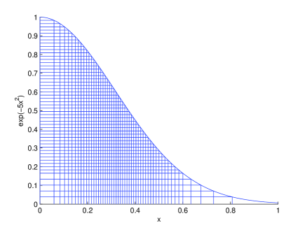
Figure 2: Adaptive grid for the sparse QCP interpolation.

The sparse interpolation in the QCP format requires the information of the function only at $M\,(\sim 2Lr)$ points instead of the information at the full set $2^{L}$ of grid points. The overall computational complexity of the algorithm is reduced dramatically and it is $O(M)$ per iteration step of the ALS algorithm. Here $M\ll N=2^{L}.$ In the above numerical example the sampling points were chosen randomly. Clearly, there are many strategies for adaptive selection of sampling points based on some a priori knowledge about the behavior of the underlying function, but this issue will not be discussed here in detail. Figure 2 shows an example of the adaptive choice of the interpolation grid for the function $e^{-5x^{2}}$. Notice that the so-called TT-cross approximation in the TT format [33] requires asymptotically smaller number of functional calls than $N$ in the case of large enough $N$.

6 Conclusions and future work

In this article, the ALS-type algorithms for approximation/interpolation of a function in QCP format have been described. The representation complexity of the rank-$r$ QCP format is estimated by $2Lr$. As commented in section 3, the condition numbers of the matrices appearing in each iteration of the ALS algorithm are large for large values of the rank $r.$ Complete data of the tensor has been used to obtain the CP approximation at the computational cost $O(2^{L-1})$ per iteration. This complexity is reduced if the approximation can be obtained using only a few data points, which can be viewed as the sparse interpolation of a given function in the QCP format.

The idea of obtaining CP approximation using only small number of functional calls is described and numerical examples are presented. In this case the overall computational complexity of the QCP approximation is only $O(2Lr)$ per iteration step of the algorithm, i.e., it is proportional to the number of representation parameters in the target QCP tensor. It is remarkable that the complexity of the QCP interpolation scales linearly in the CP rank and logarithmically in the full vector size.

A discussion of different strategies for clever choice of the sampling points as well as the error analysis of the method and the extension of the algorithm to functions of two or three variables is postponed to ongoing work. The QCP format can be used in the approximation of the solution of PDEs, integration of highly oscillating functions and to approximate functions where the calculation of function values is computationally expensive. This format can also be used to just represent functions that depend on many parameters.

Acknowledgements. KKN appreciates the support provided by the Max-Planck Institute for Mathematics in the Sciences (Leipzig, Germany) during his scientific visit in 2015. The authors are thankful to Dr. V. Khoromskaia (MPI MIS, Leipzig) for useful discussions.

Appendix

A1. Kronecker product

Let $A$ be an $m\times n$ matrix and $B$ be an $p\times q$ matrix, then the Kronecker product $A\otimes B$ is an $mp\times nq$ block matrix:

$$A\otimes B=\left[\begin{array}[]{cccc}a_{11}B&a_{12}B&...&a_{1n}B\\ a_{21}B&a_{22}B&...&a_{2n}B\\ \\ a_{m1}B&a_{m2}B&...&a_{mn}B\end{array}\right].$$

Properties of the Kronecker product

For matrices $B,C,D$ and $F$ of suitable sizes the following properties hold:

P1. $(B\otimes C)^{T}=B^{T}\otimes C^{T}.$
P2. $(B\otimes C)\otimes D=B\otimes(C\otimes D).$
P3. $(B\otimes C)(D\otimes F)=BD\otimes CF.$
P4. $(B\otimes C)^{-1}=B^{-1}\otimes C^{-1}.$

A2. Khatri-Rao product

Let $B=[\mathbf{b}_{1}|\mathbf{b}_{2}|\ldots|\mathbf{b}_{r}]\in\mathbb{R}^{n_{1}\times r},$ where $\mathbf{b}_{1},\mathbf{b}_{2},\ldots,\mathbf{b}_{r}$ are the columns of the matrix $B.$ Let $C=[\mathbf{c}_{1}|\mathbf{c}_{2}|\ldots|\mathbf{c}_{r}]\in\mathbb{R}^{n_{2}\times r}.$ The Khatri-Rao product of $B$ and $C$ is defined as the $n_{1}n_{2}\times r$ matrix $\displaystyle B\odot C=[\mathbf{b}_{1}\otimes\mathbf{c}_{1}|\mathbf{b}_{2}\otimes\mathbf{c}_{2}|\ldots|\mathbf{b}_{r}\otimes\mathbf{c}_{r}].$ Here $\mathbf{b}_{i}\times\mathbf{c}_{i}$ is $\displaystyle\mathbf{b}_{i}\otimes\mathbf{c}_{i}=\left[\begin{array}[]{c}b_{1i}\\ b_{2i}\\ \vdots\\ b_{n_{1}i}\end{array}\right]\otimes c_{i}=\left[\begin{array}[]{c}b_{1i}c_{i}\\ b_{2i}c_{i}\\ \vdots\\ b_{n_{1}i}c_{i}\end{array}\right]=\left[\begin{array}[]{c}b_{1i}c_{1i}\\ b_{1i}c_{2i}\\ \vdots\\ b_{1i}c_{n_{2}i}\\ b_{2i}c_{1i}\\ \vdots\\ b_{n_{1}i}c_{n_{2}i}\end{array}\right].$

$O(n_{1}n_{2}r)$ arithmetic operations are required to compute $B\odot C.$

A3. Rank 2 canonical approximation of a $4^{th}$ order tensor

Consider a $4^{th}$ order tensor. Imagine that the tensor is generated by reshaping a vector $\mathbf{x}=[\tau_{1},\,\tau_{2},\,\tau_{3},\ldots,\tau_{16}]^{T}$ of length 16. Let $\chi=reshape(\mathbf{x},2,2,2,2).$

We obtain a rank two canonical approximation to the tensor $\chi$ using ALS. The rank-2 approximation in canonical format is given by

$$\chi\cong\left(\begin{array}[]{c}a_{1}^{1}\\ a_{2}^{1}\end{array}\right)\otimes\left(\begin{array}[]{c}b_{1}^{1}\\ b_{2}^{1}\end{array}\right)\otimes\left(\begin{array}[]{c}c_{1}^{1}\\ c_{2}^{1}\end{array}\right)\otimes\left(\begin{array}[]{c}d_{1}^{1}\\ d_{2}^{1}\end{array}\right)+\left(\begin{array}[]{c}a_{1}^{2}\\ a_{2}^{2}\end{array}\right)\otimes\left(\begin{array}[]{c}b_{1}^{2}\\ b_{2}^{2}\end{array}\right)\otimes\left(\begin{array}[]{c}c_{1}^{2}\\ c_{2}^{2}\end{array}\right)\otimes\left(\begin{array}[]{c}d_{1}^{2}\\ d_{2}^{2}\end{array}\right).$$

To obtain the rank-2 canonical approximation, we minimize the functional $\mathcal{F}$

$$\mathcal{F}=\frac{1}{2}\left\|\chi-\left(\begin{array}[]{c}a_{1}^{1}\\ a_{2}^{1}\end{array}\right)\otimes\left(\begin{array}[]{c}b_{1}^{1}\\ b_{2}^{1}\end{array}\right)\otimes\left(\begin{array}[]{c}c_{1}^{1}\\ c_{2}^{1}\end{array}\right)\otimes\left(\begin{array}[]{c}d_{1}^{1}\\ d_{2}^{1}\end{array}\right)+\left(\begin{array}[]{c}a_{1}^{2}\\ a_{2}^{2}\end{array}\right)\otimes\left(\begin{array}[]{c}b_{1}^{2}\\ b_{2}^{2}\end{array}\right)\otimes\left(\begin{array}[]{c}c_{1}^{2}\\ c_{2}^{2}\end{array}\right)\otimes\left(\begin{array}[]{c}d_{1}^{2}\\ d_{2}^{2}\end{array}\right)\right\|_{F}^{2}$$

$$=\frac{1}{2}\,\left(\left(\tau_{1}-\!(a_{1}^{1}b_{1}^{1}c_{1}^{1}d_{1}^{1}\!+\!a_{1}^{2}b_{1}^{2}c_{1}^{2}d_{1}^{2})\right)^{2}+\!\left(\tau_{2}-\!(a_{2}^{1}b_{1}^{1}c_{1}^{1}d_{1}^{1}\!+\!a_{2}^{2}b_{1}^{2}c_{1}^{2}d_{1}^{2}\right)^{2}+\ldots+\!\left(\tau_{16}-\!(a_{2}^{1}b_{2}^{1}c_{2}^{1}d_{2}^{1}\!+\!a_{2}^{2}b_{2}^{2}c_{2}^{2}d_{2}^{2}\right)^{2}\right).$$

Let us denote

$$A=\left[\begin{array}[]{cc}a_{1}^{1}&a_{1}^{2}\\ a_{2}^{1}&a_{2}^{2}\end{array}\right],\,B=\left[\begin{array}[]{cc}b_{1}^{1}&b_{1}^{2}\\ b_{2}^{1}&b_{2}^{2}\end{array}\right],\,C=\left[\begin{array}[]{cc}c_{1}^{1}&c_{1}^{2}\\ c_{2}^{1}&c_{2}^{2}\end{array}\right]\,\,\textrm{and}\,\,D=\left[\begin{array}[]{cc}d_{1}^{1}&d_{1}^{2}\\ d_{2}^{1}&d_{2}^{2}\end{array}\right].$$

By ALS, $\mathcal{F}$ is minimized in an alternating way. ALS first fixes $B,\,C$ and $D$ to minimize for $A,$ then fixes $A,\,C$ and $D$ to minimize for $B$, then fixes $A,\,B$ and $D$ to minimize for $C$ and finally fixes $A,\,B$ and $C$ to minimize for $D.$ Since we are fixing all but one direction in each step of an iteration, the problem reduces to a linear least-squares problem. All the steps of one iteration are described below.

Step 1: Fix $B,C$ and $D$ and solve for $A.$ The minimization leads to the equations

$$\frac{\partial\mathcal{F}}{\partial a_{1}^{1}}=0,\frac{\partial\mathcal{F}}{\partial a_{1}^{2}}=0\quad\text{and}\quad\frac{\partial\mathcal{F}}{\partial a_{2}^{1}}=0,\frac{\partial\mathcal{F}}{\partial a_{2}^{2}}=0,$$

which give a decoupled diagonal system

$$\left[\begin{array}[]{cc}\hat{A}^{T}\hat{A}&0\\ 0&\hat{A}^{T}\hat{A}\end{array}\right]\left[\begin{array}[]{c}\left[\begin{array}[]{c}a_{1}^{1}\\ a_{1}^{2}\end{array}\right]\\ \left[\begin{array}[]{c}a_{2}^{1}\\ a_{2}^{2}\end{array}\right]\end{array}\right]=\left[\begin{array}[]{c}\hat{A}^{T}\chi(1,:,:,:)\\ \hat{A}^{T}\chi(2,:,:,:)\end{array}\right],$$ (59)

where (see A2)

$$\hat{A}=\left[\begin{array}[]{cc}d_{1}^{1}c_{1}^{1}b_{1}^{1}&\,\,\,d_{1}^{2}c_{1}^{2}b_{1}^{2}\\ d_{1}^{1}c_{1}^{1}b_{2}^{1}&\,\,\,d_{1}^{2}c_{1}^{2}b_{2}^{2}\\ d_{1}^{1}c_{2}^{1}b_{1}^{1}&\,\,\,d_{1}^{2}c_{2}^{2}b_{1}^{2}\\ d_{1}^{1}c_{2}^{1}b_{2}^{1}&\,\,\,d_{1}^{2}c_{2}^{2}b_{2}^{2}\\ d_{2}^{1}c_{1}^{1}b_{1}^{1}&\,\,\,d_{2}^{2}c_{1}^{2}b_{1}^{2}\\ d_{2}^{1}c_{1}^{1}b_{2}^{1}&\,\,\,d_{2}^{2}c_{1}^{2}b_{2}^{2}\\ d_{2}^{1}c_{2}^{1}b_{1}^{1}&\,\,\,d_{2}^{2}c_{2}^{2}b_{1}^{2}\\ d_{2}^{1}c_{2}^{1}b_{2}^{1}&\,\,\,d_{2}^{2}c_{2}^{2}b_{2}^{2}\end{array}\right]=D\odot C\odot B,\quad\chi(1,:,:,:)=\left[\begin{array}[]{c}\tau_{1}\\ \tau_{3}\\ \tau_{5}\\ \tau_{7}\\ \tau_{9}\\ \tau_{11}\\ \tau_{13}\\ \tau_{15}\end{array}\right],\quad\chi(2,:,:,:)=\left[\begin{array}[]{c}\tau_{2}\\ \tau_{4}\\ \tau_{6}\\ \tau_{8}\\ \tau_{10}\\ \tau_{12}\\ \tau_{14}\\ \tau_{16}\end{array}\right].$$ (84)

Step 2: Fix $A,C,D$ and solve for $B.$ Then the equations,

$$\frac{\partial\mathcal{F}}{\partial b_{1}^{1}}=0,\frac{\partial\mathcal{F}}{\partial b_{1}^{2}}=0\quad\textrm{and}\quad\frac{\partial\mathcal{F}}{\partial b_{2}^{1}}=0,\frac{\partial\mathcal{F}}{\partial b_{2}^{2}}=0$$

give the linear system

$$\left[\begin{array}[]{cc}\hat{B}^{T}\hat{B}&0\\ 0&\hat{B}^{T}\hat{B}\end{array}\right]\left[\begin{array}[]{c}\left[\begin{array}[]{c}b_{1}^{1}\\ b_{1}^{2}\end{array}\right]\\ \left[\begin{array}[]{c}b_{2}^{1}\\ b_{2}^{2}\end{array}\right]\end{array}\right]=\left[\begin{array}[]{c}\hat{B}^{T}\chi(:,1,:,:)\\ \hat{B}^{T}\chi(:,2,:,:)\end{array}\right]$$

with

$$\hat{B}=D\odot C\odot A\quad\text{and}\quad\chi(:,1,:,:)=\left[\begin{array}[]{c}\tau_{1}\\ \tau_{2}\\ \tau_{5}\\ \tau_{6}\\ \tau_{9}\\ \tau_{10}\\ \tau_{13}\\ \tau_{14}\end{array}\right],\quad\chi(:,2,:,:)=\left[\begin{array}[]{c}\tau_{3}\\ \tau_{4}\\ \tau_{7}\\ \tau_{8}\\ \tau_{11}\\ \tau_{12}\\ \tau_{15}\\ \tau_{16}\end{array}\right].$$ (104)

Step 3: Fix $A,B,D$ and solve for $C.$ Then the equations

$$\frac{\partial\mathcal{F}}{\partial c_{1}^{1}}=0,\frac{\partial\mathcal{F}}{\partial c_{1}^{2}}=0\quad\textrm{and}\quad\frac{\partial\mathcal{F}}{\partial c_{2}^{1}}=0,\frac{\partial\mathcal{F}}{\partial c_{2}^{2}}=0$$

give the linear system

$$\left[\begin{array}[]{cc}\hat{C}^{T}\hat{C}&0\\ 0&\hat{C}^{T}\hat{C}\end{array}\right]\left[\begin{array}[]{c}\left[\begin{array}[]{c}c_{1}^{1}\\ c_{1}^{2}\end{array}\right]\\ \left[\begin{array}[]{c}c_{2}^{1}\\ c_{2}^{2}\end{array}\right]\end{array}\right]=\left[\begin{array}[]{c}\hat{C}^{T}\chi(:,:,1,:)\\ \hat{C}^{T}\chi(:,:,2,:)\end{array}\right]$$

with

$$\hat{C}=D\odot B\odot A\quad\textrm{and}\quad\chi(:,:,1,:)=\left[\begin{array}[]{c}\tau_{1}\\ \tau_{2}\\ \tau_{3}\\ \tau_{4}\\ \tau_{9}\\ \tau_{10}\\ \tau_{11}\\ \tau_{12}\end{array}\right],\quad\chi(:,:,2,:)=\left[\begin{array}[]{c}\tau_{5}\\ \tau_{6}\\ \tau_{7}\\ \tau_{8}\\ \tau_{13}\\ \tau_{14}\\ \tau_{15}\\ \tau_{16}\end{array}\right].$$ (124)

Step 4: Fix $A,B,C$ and solve for $D.$ The equations

$$\frac{\partial\mathcal{F}}{\partial d_{1}^{1}}=0,\frac{\partial\mathcal{F}}{\partial d_{1}^{2}}=0\quad\textrm{and}\quad\frac{\partial\mathcal{F}}{\partial d_{2}^{1}}=0,\frac{\partial\mathcal{F}}{\partial d_{2}^{2}}=0$$

give the linear system

$$\left[\begin{array}[]{cc}\hat{D}^{T}\hat{D}&0\\ 0&\hat{D}^{T}\hat{D}\end{array}\right]\left[\begin{array}[]{c}\left[\begin{array}[]{c}d_{1}^{1}\\ d_{1}^{2}\end{array}\right]\\ \left[\begin{array}[]{c}d_{2}^{1}\\ d_{2}^{2}\end{array}\right]\end{array}\right]=\left[\begin{array}[]{c}\hat{D}^{T}\chi(:,:,:,1)\\ \hat{D}^{T}\chi(:,:,:,2)\end{array}\right]$$

with

$$\hat{D}=C\odot B\odot A\quad\textrm{and}\quad\chi(:,:,:,1)=\left[\begin{array}[]{c}\tau_{1}\\ \tau_{2}\\ \tau_{3}\\ \tau_{4}\\ \tau_{5}\\ \tau_{6}\\ \tau_{7}\\ \tau_{8}\end{array}\right],\quad\chi(:,:,:,2)=\left[\begin{array}[]{c}\tau_{9}\\ \tau_{10}\\ \tau_{11}\\ \tau_{12}\\ \tau_{13}\\ \tau_{14}\\ \tau_{15}\\ \tau_{16}\end{array}\right].$$ (144)

Here the matrices $\hat{A,}\hat{B,}\hat{C}$ and $\hat{D}$ are of size $8\times 2.$ This is $2^{4-1}\times r$ where $r=2.$ But the matrices like $\hat{A}^{T}A$ appearing in the decoupled linear systems are of very small size $2\times 2$ for $r=2.$ Also one can see that the matrices $\hat{A}^{T}\hat{A},\,\hat{B}^{T}\hat{B},\,\hat{C}^{T}\hat{C},\,\hat{D}^{T}\hat{D}$ are symmetric and positive definite.

References

- [1] P. Benner, S. Dolgov, V. Khoromskaia and B. N. Khoromskij, Fast iterative solution of the Bethe-Salpeter eigenvalue problem using low-rank and QTT tensor approximation, Journal of Computational Physics, 334, 221-239, 2017.
- [2] J. D. Carroll and J. J. Chang, Analysis of individual differences in multidimensional scaling via an N-way generalization of ‘Eckart-Young’ decomposition, Psychometrika, 35, 283–319, 1970.
- [3] P. Common, X. Luciani and A. L. F. de Almeida, Tensor decomposition, Alternating least squares and other tales, Journal of Chemometrics, 23, 393-405, 2009.
- [4] A. Cichocki, N. Lee, I. Oseledets, A.H. Phan, Q. Zhao and D.P. Mandic, Tensor Networks for Dimensionality Reduction and Large-scale Optimization: Part 1 Low-Rank Tensor Decompositions, Foundations and Trends in Machine Learning, 9 (4–5), 249–429, 2016.
- [5] S.V. Dolgov and B.N. Khoromskij, Two-level Tucker-TT-QTT format for optimized tensor calculus, SIAM J. on Matr. Anal. Appl., 34(2), 593-623, 2013.
- [6] Sergey Dolgov, Boris N. Khoromskij, Alexander Litvinenko, and Hermann G. Matthies. Computation of the Response Surface in the Tensor Train data format. SIAM/ASA J. Uncertainty Quantification, 2015, Vol. 3, pp. 1109-1135.
- [7] I. Domanov, Study of Canonical Polyadic decomposition of higher order tensors, Doctoral thesis, KU Leuven, 2013.
- [8] M. Espig, W. Hackbusch and A. Khachatryan, On the convergence of alternating least squares optimisation in tensor format representations, Preprint, 423, RWTH, Achen, May 2015.
- [9] G. H. Golub and C. F. Van Loan, Matrix computations, 4th edition, Johns Hopkins Studies in the Mathematical Sciences, 2013.
- [10] L. Grasedyck, D. Kressner and C. Tobler, A literature survey of low-rank tensor approximation techniques, GAMM-Mitteilungen, 36(1), 53-78, 2013.
- [11] W. Hackbusch, Tensor spaces and numerical tensor calculus, Springer, Berlin, 2012.
- [12] R. A. Harshman, Foundations of the PARAFAC procedure: Models and conditions for an “explanatory” multi-model factor analysis, UCLA Working Papers in Phonetics, 16, 1–84, 1970. http://publish.uwo.ca/ $sim$harshman/wpppfac0.pdf.
- [13] V. Kazeev, I. Oseledets, M. Rakhuba and Ch. Schwab, QTT-finite-element approximation for multiscale problems I: model problems in one dimension, Adv. Comput. Math., 43(2), 411-442, 2017.
- [14] V. Kazeev, O. Reichmann, and Ch. Schwab. Low-rank tensor structure of linear diffusion operators in the TT and QTT formats. Linear Algebra and its Applications, v. 438(11), 2013, 4204-4221.
- [15] T. G. Kolda and B. W. Bader, Tensor decompositions and applications, SIAM Review, 51(3), 455-500, 2009.
- [16] B.N. Khoromskij, -Quantics Approximation of - Tensors in High-Dimensional Numerical Modeling, J. Constr. Approx., 34(2), 257-289, 2011.
- [17] B.N. Khoromskij, Tensors-structured Numerical Methods in Scientific Computing: Survey on Recent Advances, Chemometr. Intell. Lab. Syst. 11, 1-19, 2012.
- [18] Boris N. Khoromskij. Tensor Numerical Methods for High-dimensional PDEs: Basic Theory and Initial Applications. ESAIM: Proceedings and Surveys, 2015, Vol. 48, p. 1-28.
- [19] B. N. Khoromskij and I. Oseledets, Quantics-TT Collocation approximation of parameter-dependent and stochastic elliptic PDEs, Comp. Meth. in Applied Math., 10(4), 376-394, 2010.
- [20] B. N. Khoromskij and I. Oseledets, Quantics-TT approximation of elliptic solution operators in higher dimensions, Russ. J. Numer. Anal. Math. Modelling, 26(3), 303-322, 2011.
- [21] B. N. Khoromskij and S. Repin, A fast iteration method for solving elliptic problems with quasiperiodic coefficients, Russ. J. Numer. Anal. Math. Modelling, 30 (6), 329-344, 2015. E-preprint arXiv:1510.00284, 2015.
- [22] B. N. Khoromskij and Ch. Schwab, Tensor-Structured Galerkin Approximation of Parametric and Stochastic Elliptic PDEs, SIAM J. Sci. Comput., 33(1), 1-25, 2011.
- [23] V. Khoromskaia and B. N. Khoromskij, Grid-based lattice summation of electrostatic potentials by assembled rank-structured tensor approximation, Comp. Phys. Comm., 185, 3162-3174, 2014.
- [24] V. Khoromskaia and B. N. Khoromskij, Tensor numerical methods in quantum chemistry: from Hartree-Fock to excitation energies, Phys. Chem. Chem. Phys., 17, 31491-31509, 2015.
- [25] V. Khoromskaia, B. N. Khoromskij and R. Schneider, QTT Representation of the Hartree and Exchange Operators in Electronic Structure Calculations, Comp. Meth. in Applied Math., 11(3), 327-341, 2011.
- [26] B.N. Khoromskij, S. Sauter, and A. Veit. Fast Quadrature Techniques for Retarded Potentials Based on TT/QTT Tensor Approximation. Comp. Meth. in Applied Math., v.11 (2011), No. 3, 342 - 362.
- [27] Na Li, S. Kindermann and C. Navasca, Some Convergence results on the regularized alternating least-squares method for tensor decomposition, Lin. Alg. and Appl., 438(2), 796-812, 2013 .
- [28] C. Navasca, L. D. Lathauwer and S. Kindermann, Swamp reducing technique for tensor decompositions, EUSIPCO 2008.
- [29] K.K. Naraparaju and J. Schneider, Literature survey on low rank approximation of matrices. Lin. Multilin. Alg., DOI 10.1080/03081087.2016.1267104
- [30] I. V. Oseledets, Approximation of matrices using tensor decomposition, SIAM J. Matrix Anal. Appl., 31(4), 2130-2145, 2010.
- [31] I. V. Oseledets, Tensor-Train decomposition, SIAM J. of Sci. Computing, 33(5), 2295-2317, 2011.
- [32] I.Oseledets, D. Savostyanov, E.Tyrtyshnikov, Linear algebra for tensor problems, Computing, 85 (2009), 169–188.
- [33] I.V. Oseledets, and E.E. Tyrtyshnikov. TT-Cross Approximation for Multidimensional arrays. Liner Algebra Appl. 432(1), 70-88 (2010).
- [34] Th. Rohwedder, S. Holtz, and R. Schneider, The alternation least square scheme for tensor optimisation in the TT-format. Preprint DGF-Schwerpunktprogramm 1234 71, 2010.
- [35] A. Uschmajew, Local convergence of the alternative least squares algorithm for canonical tensor approximation, SIAM J. Mat. Anal. App., 33(2), 639-652, 2012.
- [36] C. F. Van Loan, Lectures, http://issnla2010.ba.cnr.it/Course_Van_Loan.htm.