A local target-specific QBX method for Laplace’s equation in 3D multiply-connected domains.

A local target specific quadrature by expansion method for evaluation of layer potentials in 3D

Abstract

Accurate evaluation of layer potentials is crucial when boundary integral equation methods are used to solve partial differential equations. Quadrature by expansion (QBX) is a recently introduced method that can offer high accuracy for singular and nearly singular integrals, using truncated expansions to locally represent the potential. The QBX method is typically based on a spherical harmonics expansion which when truncated at order $p$ has $O(p^{2})$ terms. This expansion can equivalently be written with $p$ terms, however paying the price that the expansion coefficients will depend on the evaluation/target point. Based on this observation, we develop a target specific QBX method, and apply it to Laplace’s equation on multiply-connected domains. The method is local in that the QBX expansions only involve information from a neighborhood of the target point. An analysis of the truncation error in the QBX expansions is presented, practical parameter choices are discussed and the method is validated and tested on various problems.

Keywords: Layer potentials; integral equations; quadrature by expansion; exterior Dirichlet problem; spherical harmonics expansions; multiply-connected domain

1 Introduction

Numerical methods based on boundary integral equations have the advantage that only the boundaries of the domain must be discretized, which both simplifies the handling of the geometry and reduces the number of discretization points. The resulting linear system after discretization is however dense, and the evaluation of layer potentials requires accurate quadrature methods for singular and nearly singular integrals. Nearly singular integrals arise when evaluating solutions close to boundaries during a post-processing step, after the integral equation has already been solved. They also arise in problems involving multiply-connected domains, when the integral equation is to be solved and separate boundary components are nearly touching. Such problems are important in applications including, for example, electromagnetic scattering in media with multiple inclusions and particle Stokes flow.

With a discretization based on a second kind integral equation, the resulting matrix is well conditioned, with a condition number independent on the fineness of the discretization. The number of iterations in an iterative method such as GMRES hence stays constant as the discretization of the boundaries is refined, yielding a total cost of $O(N^{2})$ to solve the system, where $N$ is the number of unknowns. The $O(N^{2})$ comes from the cost of the matrix-vector multiply for a full matrix, and can be reduced to $O(N)$ or $O(N\log N)$ using a fast method, such as the fast multipole method (FMM) [12], or an FFT based method such as a fast Ewald method (commonly for periodic problems [24], recently also for non-periodic ones [16]).

Regarding efficient and accurate quadrature methods for the evaluation of singular and nearly singular integrals, excellent methods that utilize a complex variable formulation are available in two dimensions [4, 14, 26]. Considering arbitrary geometries in three dimensions, this remains a topic of current research where several methods have been introduced and contributed different advances [5, 7, 8, 31, 32, 33].

Quadrature by expansion (QBX) is a rather recent method [3, 21] for the numerical evaluation of singular and nearly singular integrals. It was introduced for the Helmholtz kernel in two dimensions, but the central principle of the method can be generalized to other kernels in both two and three dimensions. Noting that the layer potential is smooth away from the boundary, it can locally be represented using an expansion centered about a point or expansion center which is located just off the surface. Once the coefficients of this expansion have been computed, the potential can be evaluated at a target point closer to the surface, or even on the boundary [10] using this local expansion (see Figure 1). Such expansions are used also in the FMM, and it is hence attractive to integrate the QBX method into an FMM. In [28], a first such step is taken in two dimensions. There, the QBX method is “global”, meaning that all information from all boundaries will enter each QBX local expansion before evaluation. Localizing the QBX treatment by using only information from boundaries that are near the expansion center would reduce the cost, but introduces other algorithmical challenges, even more so in three dimensions.

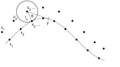
Figure 1: QBX with expansion centers $\mathbf{c}_{1},\mathbf{c}_{2},\ldots$ and targets $\mathbf{x}_{1},\mathbf{x}_{2},\ldots$. The domain of convergence for the expansion has radius $r_{c}$, and $\theta$ is defined in (19).

In [18], a QBX method was presented for spheroidal particles in three-dimensional Stokes flow. Whenever an evaluation point is on or close to a spheroidal surface, a QBX expansion is used to evaluate the layer potential over that surface. Contributions from different surfaces are kept separate, even if the surfaces are close. Once QBX centers have been chosen relative to the surface, precomputations can be made to strongly accelerate the computation of the QBX coefficients. Using the axisymmetry of the body, the storage need can be greatly reduced, and the same precomputed values can be used for all spheroids of the same shape. This method is combined with an FFT based Ewald summation method - the Spectral Ewald method [17, 23], and yields an $O(N\log N)$ method (with $N$ the total number of gridpoints) as the number of spheroids is increased while the resolution on each spheroid is kept fixed.

The error in the QBX method for evaluating a layer potential on or close to the boundary has two main sources: the error from truncation of the local series expansion and the computation of the expansion coefficients. The truncation error was analyzed by Epstein et al. [10] for the Laplace and Helmholtz kernels in two and three dimensions, assuming a “global” QBX approach. The error due to computations of the expansion coefficients is again a quadrature error in evaluating the integrals defining these coefficients. This was analyzed in [19] using a method based on contour integration and calculus of residues in two dimensions and for some three dimensional cases. Once a procedure for taking the panel shape into account is introduced, the error estimates in 2D are remarkably precise, and allow for the development of an adaptive QBX method where parameters are selected automatically, given an error tolerance [20].

In this paper, we consider the Laplace’s equation in multiply- connected domains in three dimensions, and we focus on the further development of a QBX based method. In contrast to [18], we assume no specific shapes of the boundaries other than that they are smooth, but we will not take on the daunting task of integrating QBX into a FMM framework for a general three dimensional problem. Instead, we view the QBX technique as a local correction. We divide the surface into panels, and only for panels close to the evaluation point will the QBX approach be applied, for other panels the integral is well resolved using regular quadrature. This local point of view is not new, and versions of a local QBX method have been developed for 2D problems in [3], [27]. In extending this idea to 3D, it is essential that the number of terms in the QBX expansion is as small as possible. We however do not need a separation between source and target in these expansions, which is essential e.g. for the FMM. Therefore, we will use a target specific QBX expansion, that will need $p$ terms to achieve the same accuracy as a spherical harmonics expansion with $p^{2}$ terms.

We refer to the method that we have developed as a local target-specific QBX method. Its main significance is that it can compute both singular and nearly singular integrals for general surfaces in 3D with high accuracy and $O(p\cdot N)$ complexity. Even though we are considering Laplace’s equation in this paper, the method may also be extended for the accurate evaluation of single and double layer potentials arising in other boundary value problems, such as potential flow, Stokes flow, electromagnetics, or elasticity. One main motivation for developing this method is to efficiently and accurately evaluate nearly singular integrals for a time-dependent geometry where precomputation is not possible (although the method presented here makes use of precomputation, it is not necessary). This can involve interacting drops, vesicles or blood cells, where the geometry is changing due to the movement and deformation of these objects, and where accurate evaluation of nearly singular integrals is needed to resolve close interactions.

The principal results justifying our use of a local QBX expansion scheme are the analyses of the two main sources of error, truncation and coefficient error, presented in Section 5. There, we provide new estimates for the truncation error of the series expansion of a local layer potential for the Laplace kernel in 3D (in contrast to the global layer potentials analyzed in [10]). We also make use of the analysis in [19] to quantify the quadrature error in computing the QBX expansion coefficients. This latter error will be called the coefficient error. Crucially, the estimates highlight the interplay between the grid size $h$, the distance $r_{c}$ of the expansion centers from the boundary, and the order of truncation $p$ on the accuracy of our method. The error estimates also give a rational basis for the choice of numerical parameters.

The method presented here can be made to have $O(N)$ complexity, where $N$ is the total number of target points, by scaling the size of the local correction patch so that it has a constant number of source points as $N$ grows. Optimal complexity is then achieved by combining our local QBX method with a fast hierarchical method, such as the Fast Multipole Method, to compute the contribution to the layer potential from source points that are outside of the local correction patch (see §6.3). One advantage of this approach is that by decoupling the FMM from the QBX expansions the algorithm allows for the use of pre-existing or standard FMM software, and is greatly simplified. We will see that for this scaling, the coefficient and truncation errors remain fixed as $N$ increases, but can be made controllably small. Used in this way our QBX method is not classically convergent, but has controlled precision [21]. A classically convergent scheme can be achieved by letting the number of local patch points grow (even slowly) with $N$, at the expense of optimal complexity.

The rest of this paper is as follows. We start by giving the problem statement and the integral equations in §2. Surprisingly enough, we could not find a derivation in the literature of a uniquely solvable second kind integral equation for the multiply-connected external Dirichlet problem in three dimensions, and we will here provide a brief derivation. In §3, we introduce the surface discretization and the regular quadrature rules, before we describe the local target specific QBX expansions in §4. Results from our error analysis are presented in §5. A description of the full algorithm is given in §6, before we turn to presenting the numerical results in §7.

2 Problem statement, layer potentials and the integral equations

Let $D_{1},\ldots,D_{M}$ be a collection of disjoint, bounded, and open regions in $\mathbb{R}^{3}$, each with $C^{2}$ connected boundary $\partial D_{j}$, and let $D=D_{1}\cup\ldots D_{M}$. We consider the Dirichlet problem for Laplace’s equation

$$\nabla^{2}u = 0~{}~{}~{}\mbox{in the interior or exterior of }D$$ (1)

$$u = f~{}~{}\mbox{on}~{}~{}\partial D$$ (2)

for continuous boundary data $f$. For the exterior problem, it is required that $u(\mathbf{x})\rightarrow 0$ uniformly in all directions.

It is well known that each of these boundary value problems has a unique solution which depends continuously on the boundary data. We now want to formulate the integral equations for solving both the interior and exterior Dirichlet problem. We wish to have a second kind integral equation which will yield a well-conditioned discrete problem. This is straight forward for the interior problem, but much less so for the exterior problem, and we therefore start by presenting this formulation. In doing so, we will need to introduce layer potentials and jump relations [22].

Let

$$G(\mathbf{x},\mathbf{y})=\frac{1}{4\pi}\frac{1}{|\mathbf{x}-\mathbf{y}|}$$

be the fundamental solution or free-space Green’s function for Laplace’s equation in $\mathbb{R}^{3}$. Given a function $\sigma$ which is continuous on the boundary $\partial D$ of a region $D$, the functions

$$u(\mathbf{x})=\mathcal{S}\sigma(\mathbf{x})=\int_{\partial D}\sigma(\mathbf{y})G(\mathbf{x},\mathbf{y})\ dS_{\mathbf{y}},~{}~{}~{}\mathbf{x}\in\mathbb{R}^{3}\backslash\partial D,$$ (3)

and

$$v(\mathbf{x})=\mathcal{D}\sigma(\mathbf{x})=\int_{\partial D}\sigma(\mathbf{y})\frac{\partial G(\mathbf{x},\mathbf{y})}{\partial\nu(\mathbf{y})}\ dS_{\mathbf{y}},~{}~{}~{}\mathbf{x}\in\mathbb{R}^{3}\backslash\partial D,$$ (4)

are called, respectively, the single layer and double layer potential with density $\sigma$. In the above, $\nu(\mathbf{x})$ is the outward normal at a point $\mathbf{x}\in\partial D$, that is, pointing into the exterior domain $\mathbb{R}^{3}\backslash\bar{D}$.

The single and double layer potentials represent harmonic functions in $D$ and $\mathbb{R}^{3}\backslash\bar{D}$. They are used to represent solutions to boundary value problems for Laplace’s equation, with the density $\sigma(\mathbf{y})$ determined by the boundary data. The solution to the Dirichlet problem can be written in terms of the double layer potential alone, while the single layer potential applies to the Neumann problem (there are also combined representations involving both the single and double layer). For concreteness, we focus on the Dirichlet problem and henceforth our QBX method will be described for the double layer potential. Analogous methods for the single layer potential follow with obvious modifications.

The layer potentials become singular on the boundary $\partial D$ and are difficult to evaluate accurately by a numerical method, not only when the evaluation or target point $\mathbf{x}$ is on the boundary $\partial D$, but also when it is close to the boundary and the integral is nearly singular. If we let $\mathbf{x}$ approach the boundary from either the interior or exterior domain for the double layer potential, the limits are different. This is expressed by the following jump relation [22] that will be used in our formulation:

Theorem 2.1.

Under the given assumptions on $\partial D$ and $\sigma$, the double layer potential $v$ with density $\sigma$ can be continuously extended from $D$ to $\bar{D}$ and from $\mathbb{R}^{3}\backslash\bar{D}$ to $\mathbb{R}^{3}\backslash{D}$ with limiting values

$$v_{\pm}(\mathbf{x})=\int_{\partial D}\sigma(\mathbf{y})\frac{\partial G(\mathbf{x},\mathbf{y})}{\partial\nu(\mathbf{y})}\ dS_{\mathbf{y}}\pm\frac{1}{2}\sigma(\mathbf{x}),~{}~{}~{}\mathbf{x}\in\partial D,$$ (5)

where

$$v_{\pm}(\mathbf{x})=\lim_{h\rightarrow 0}v(\mathbf{x}\pm h\nu(\mathbf{x}))),$$

$\nu(\mathbf{x})$ is the outward normal at a point $\mathbf{x}\in\partial D$, and the integral exists as an improper integral.

2.1 Integral equation formulation

Consider the exterior Dirichlet problem for a multiply-connected domain. Let $v(\mathbf{x})=\mathcal{D}\sigma(\mathbf{x})$, where $\mathcal{D}$ defines the double layer potential, as in (4). The jump relation (5) provides a second kind integral equation for the density $\sigma$

$$\frac{\sigma(\mathbf{x})}{2}+\mathcal{D}\sigma(\mathbf{x})=f(\mathbf{x})~{}~{}\mbox{for}~{}~{}\mathbf{x}\in\partial D,$$ (6)

where we associate the function $v_{+}(\mathbf{x})$ in (5) with the Dirichlet data $f$. The homogeneous version of this equation is

$$\left(\frac{1}{2}+\mathcal{D}\right)\sigma(\mathbf{x})=0~{}~{}\mbox{for}~{}~{}\mathbf{x}\in\partial D.$$ (7)

Unfortunately, the above equation has nontrivial solutions, for example, $\sigma_{k}=\chi_{k}$ where $\chi_{k}$ is the characteristic function on boundary component $\partial D_{k}$. For such $\sigma_{k}$, we have from a well-known result in classical potential theory [22] that ${\cal D}\sigma_{k}(\mathbf{x})=-1/2$ if $\mathbf{x}\in\partial D_{k}$, and it immediately follows that $\sigma_{k}$ satisfies (7). Moreover, it can be shown [22] that the $M$ linearly independent functions $\sigma_{k}$ for $k=1,\ldots,M$ provide a basis for the null space of the homogeneous equation. In other words, the dimension of the null space of the homogeneous operator in (7) is equal to the number of boundary components in our domain.

We will modify the second kind integral equation (6) so that it has a unique solution (see [22] for a modified equation in the case of a single boundary component $M=1$, and [11], [15] for a similar approach in 2D). Our approach is motivated by Tausch and White [30], who considered the so-called capacitance problem, which is the adjoint of the problem considered here. Let

$$A\sigma(\mathbf{x})=\sum_{k=1}^{M}\left(\frac{1}{\sqrt{|}S_{k}|}\int_{\partial D_{k}}\sigma(\mathbf{y})\ dS_{\mathbf{y}}\right)G(\mathbf{x}_{k},\mathbf{x}),$$ (8)

where $\mathbf{x}\in\partial D$ and we recall $G$ is the free-space Green’s function. Here $\mathbf{x}_{k}$ is any point in the interior of region $D_{k}$ and

$$\left|S_{k}\right|=\int_{\partial D_{k}}dS_{\mathbf{y}}$$

is the surface area of $D_{k}$. The modified second kind equation for the density $\sigma$ is

$$\left(\frac{1}{2}+\mathcal{D}+A\right)\sigma(\mathbf{x})=f(\mathbf{x})~{}~{}\mbox{for}~{}~{}\mathbf{x}\in\partial D.$$ (9)

For the modified equation we have

Theorem 2.2.

The second kind integral equation (9) has a unique solution. Moreover, $u=(\mathcal{D}+A)\sigma$ where $\sigma$ satisfies (9) is a solution to the exterior Dirichlet problem.

Proof.

The uniqueness theorem can be established by showing that the null space of the adjoint of the second-kind operator in (9) is $\left\{0\right\}$ (by the First Fredholm Alternative [22], the dimensions of the null space of an operator and its adjoint are the same). This result follows similarly to the proof of Theorem 2.1 in [30]. To get the solution to the exterior Dirichlet problem, note that $\tilde{\mathcal{D}}\sigma=\mathcal{D}\sigma+A\sigma$ satisfies the same jump condition as $\mathcal{D}\sigma$, so $u(\mathbf{x})=\tilde{\mathcal{D}}\sigma(\mathbf{x})$ for $\mathbf{x}\in\mathbb{R}^{3}\backslash\bar{D}$, where $\sigma$ is a solution to (9), is a solution to our problem. ∎

For the exterior problem we solve (9) for $\sigma$ and find the solution for $\mathbf{x}\in\mathbb{R}^{3}\backslash\bar{D}$ by $u=(\mathcal{D}+A)\sigma$.

For the interior Dirichlet problem we again let $u(\mathbf{x})=\mathcal{D}\sigma(\mathbf{x})$, now for $\mathbf{x}\in D$. Using the jump relation (5) for the double layer potential, we obtain the integral equation

$$-\frac{\sigma(\mathbf{x})}{2}+\mathcal{D}\sigma(\mathbf{x})=f(\mathbf{x})~{}~{}\mbox{for}~{}~{}\mathbf{x}\in\partial D.$$ (10)

The homogeneous version of this integral equation has no non-trivial solution and hence does not need to be modified. This is a second kind integral equation that we need to solve for $\sigma$, and then find the solution by $u(\mathbf{x})=\mathcal{D}\sigma(\mathbf{x})$ for $\mathbf{x}\in D$.

2.2 The discrete problem

To solve the integral equation for either the interior or exterior problem, we first need a method to numerically evaluate integrals over $\partial D$, the boundary of the (possibly multiply-connected) domain. We use the notation

$$I[f]=\int_{\partial D}f(\mathbf{y})dS_{\mathbf{y}},$$

which we numerically evaluate by a quadrature rule $Q_{N}$, that defines a set of $N$ nodes $\mathbf{y}_{i}$ and weights $w_{i}$ on $\partial D$, such that

$$I[f]\approx Q_{N}[f]=\sum_{i=1}^{N}f(\mathbf{y}_{i})w_{i}.$$ (11)

Details of the quadrature we actually use will be discussed in the following two sections. Let us indicate by a superscript $h$ a quantity that is computed using $Q_{N}$, e.g.

$$\mathcal{D}^{h}\sigma(\mathbf{x})=Q_{N}\left[\sigma(\cdot)K(\mathbf{x},\cdot)\right],$$

where $K(\mathbf{x},\mathbf{y})=\nu(\mathbf{y})\cdot\nabla_{\mathbf{y}}G(\mathbf{x},\mathbf{y})$ .

We apply the Nyström method, where the integral equation is enforced at the quadrature nodes, i.e., for $\mathbf{x}_{i}=\mathbf{y}_{i}$, $i=1,\ldots,N$. The boundary integral equation for the interior problem is approximated by the $N\times N$ linear system for the density values $\sigma(\mathbf{x}_{i})$,

$$-\frac{1}{2}\sigma(\mathbf{x}_{i})+\mathcal{D}^{h}\sigma(\mathbf{x}_{i})=f(\mathbf{x}_{i}),\quad i=1,\ldots,N.$$ (12)

and similarly for the exterior problem (9),

$$\frac{1}{2}\sigma(\mathbf{x}_{i})+\mathcal{D}^{h}\sigma(\mathbf{x}_{i})+A^{h}\sigma(\mathbf{x}_{i})=f(\mathbf{x}_{i}),\quad i=1,\ldots,N.$$ (13)

where $A$ is defined in (8).

After these discrete values of $\sigma$ have been determined, the solution can be computed at any point in the domain by

$$u^{h}(\mathbf{x})=\mathcal{D}^{h}\sigma(\mathbf{x}),\quad\mathbf{x}\in D,$$ (14)

for the interior problem, and

$$u^{h}(\mathbf{x})=(\mathcal{D}^{h}+A^{h})\sigma(\mathbf{x}),\quad\mathbf{x}\in\mathbb{R}^{3}\backslash\bar{D},$$ (15)

for the exterior problem.

The matrix for the linear system ((12) or (13)) is dense, and solving it directly would incur a cost of $O(N^{3})$. For these well-conditioned formulations, the number of iterations needed in an iterative solution method such as GMRES is independent of the discretization. The problem can hence be solved at $O(N^{2})$ cost, where the constant depends on the geometry of the problem. The $O(N^{2})$ cost arise from the matrix-vector multiply for a dense system, i.e. evaluating the discretization of $\mathcal{D}^{h}\sigma$. As discussed in the introduction, applying a fast method such as a fast multipole method, a treecode or a method based on FFTs, this cost can be further reduced to $O(N)$ or $O(N\log N)$ which means that the linear system can be solved in (essentially) linear time. In the numerical examples given in Section 7, we simply use the $O(N^{2})$ direct summation to perform the matrix-vector multiply in cases that involve only a few (one or two) domains $D_{k}$. For problems with more domains, we use the $O(N\log N)$ treecode algorithm described in [25]. Details are given in Section 6.3.

3 Direct quadrature based on surface panels

Before describing our QBX scheme, we introduce a direct surface integration method based on Gauss-Legendre quadrature that will be used by our scheme. In this work, we consider as our boundaries surfaces of genus 0, that each has a parameterization in spherical coordinates

$$\partial D_{k}=\left\{\mathbf{x}(\theta,\varphi):0\leq\theta\leq{\pi},0\leq\varphi<{2\pi}\right\},k=1,\ldots,M,$$

and an integral over the surface is written as

$$\int_{\partial D_{k}}f(\mathbf{y})\,dS_{\mathbf{y}}=\int_{0}^{2\pi}\int_{0}^{\pi}f(\mathbf{y}(\theta,\varphi))W(\theta,\varphi)\ d\theta d\varphi,$$ (16)

where $W(\theta,\varphi)=|\mathbf{y}_{\theta}(\theta,\varphi)\times\mathbf{y}_{\varphi}(\theta,\varphi)|$ denotes the surface area element.

For this discretization, the $(\theta,\varphi)$ plane is for each surface $\partial D_{k}$ divided so that the surface is tiled with $N^{k}_{P}=N^{k}_{\theta}\times N^{k}_{\varphi}$ surface panels, with a total of $N_{P}$ panels over all surfaces. On each panel, we use an $q$-point Gauss-Legendre quadrature rule in both coordinate directions, and hence $q\times q$ quadrature points over the patch. This gives us a total of $N=N_{P}\times q^{2}$ quadrature points on the surfaces.

For ease of notation we can let one index cover all the quadrature points $\mathbf{y}_{i}$ and weights $w_{i}$, where $i=1,\ldots,N=q^{2}N_{p}$. Then the quadrature rule is given by (11), with the weights $w_{i}$ being the product of the surface area element $W(\mathbf{y}_{i})$ and the Gauss-Legendre quadrature weights. This quadrature rule will be referred to as the direct quadrature. We will henceforth seek the solution $\sigma$ of the discretized integral equation (13) at the quadrature points of this direct quadrature. When applied to compute the double layer potential, the direct integration $Q_{N}\left[\sigma(\cdot)K(\mathbf{x},\cdot)\right]$ or its upsampled version described in §3.1 below can be sufficiently accurate if the target point is not too close to any source panel. If it gets too close, the QBX method will be applied as a local correction (see Figure 2).

For smooth integrals, it is often advantageous to let the whole surface be only one panel, and refine the grid by increasing $q$, thereby achieving spectral accuracy. We however want to keep a locality in our discretizations, since we will modify the direct quadrature locally close to a singular or nearly singular point. In our computations, $q$ is typically set to $7$ for the direct quadrature, which gives a high order quadrature rule on each panel (15th order), without each panel becoming too large.

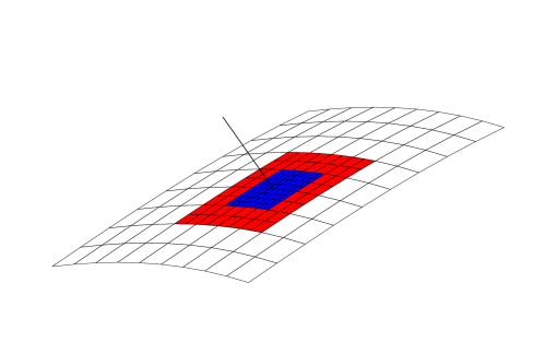
Figure 2: Tiling of the surface by Gauss-Legendre panels. In this example, ${\cal D}\sigma(\mathbf{x})$ is computed using direct quadrature over the white region, upsampled direct quadrature over the red region (with $\kappa=2$), and upsampled QBX over the blue region ($\kappa=4$).

3.1 Upsampling for quadrature

Assume that we want to evaluate an integral

$$\int_{\partial D_{k}}K(\mathbf{x},\mathbf{y})\sigma(\mathbf{y})\,dS_{\mathbf{y}}=\int_{0}^{2\pi}\int_{0}^{\pi}K(\mathbf{x},\mathbf{y}(\theta,\varphi))\sigma(\mathbf{y}(\theta,\varphi))W(\theta,\varphi)\ d\theta d\varphi,$$ (17)

where $K(\mathbf{x},\mathbf{y})$ is, e.g., the kernel of the double layer potential (4). Assume that the density $\sigma$ is known at the $N$ nodes of the direct quadrature rule. If the kernel $K$ varies rapidly and is not well resolved on that grid, a refinement can be made to increase the accuracy of the quadrature. The refinement is effective since the kernel is known analytically, but the density $\sigma$ must be interpolated and evaluated at these new points.

For a panel $P$, we denote the interpolant of $\sigma$ by $\Pi^{P}\sigma$. This interpolant is defined through the values of $\sigma$ at the $q\times q$ Gauss-Legendre points. Now, split the panel $P$ into $\kappa^{2}$ subpanels, each with $q^{2}$ Gauss-Legendre points. The values of $\Pi^{P}\sigma$ at these $\kappa^{2}q^{2}$ points can be evaluated using barycentric Lagrange interpolation [6].

We will refer to this interpolation procedure as an upsampling by a factor of $\kappa$. The upsampled quadrature of a function $f$ over a panel $P$ is a sum over all $\kappa^{2}$ sub-panels of $P$, for each one using the $q^{2}$ interpolated values of $f$. If the original quadrature over one panel is denoted $Q^{P}_{q}[f]$ then the upsampled quadrature is denoted by

$$Q^{P}_{q,\kappa}[f].$$ (18)

For the upsampled quadrature of the double layer potential $Q^{P}_{q,\kappa}[K\sigma]$, $K$ is known analytically, so as described above, this entails upsampling of $\sigma$.

4 Local expansions and the QBX method

The QBX method is used to accurately compute the double layer integrals when the source panel is close to the target point. It makes essential use of an expansion (Taylor’s, spherical harmonic, etc.) centered about a point that is located just off of the surface, but further away from the source panel than the target. To introduce the basic idea of the QBX method, we first consider expansions of the Green’s function. Introduce two points $\mathbf{x},\mathbf{y}\in{{\rm l}\kern-1.49994pt{\rm R}}^{3}$, and a point $\mathbf{c}\in{{\rm l}\kern-1.49994pt{\rm R}}^{3}$ such that $|\mathbf{x}-\mathbf{c}|<|\mathbf{y}-\mathbf{c}|$. Furthermore, let $\theta$ be the angle between $\mathbf{x}-\mathbf{c}$ and $\mathbf{y}-\mathbf{c}$ (see Figure 1). We then have the following expansion around the center $\mathbf{c}$,

$$\frac{1}{|\mathbf{x}-\mathbf{y}|}=\sum_{n=0}^{\infty}\frac{|\mathbf{x}-\mathbf{c}|^{n}\ \ }{|\mathbf{y}-\mathbf{c}|^{n+1}}P_{n}(\cos\theta),$$ (19)

where $P_{n}$ is the Legendre polynomial of degree $n$.

The addition theorem for Legendre polynomials, also called the spherical harmonics addition theorem reads

$$P_{n}(\cos\theta)=\frac{4\pi}{2n+1}\sum_{m=-n}^{n}Y_{n}^{m}(\theta_{y},\varphi_{y})Y_{n}^{-m}(\theta_{x},\varphi_{x}),$$ (20)

where $(\theta_{x},\varphi_{x})$ and $(\theta_{y},\varphi_{y})$ are the spherical coordinates of $\mathbf{x}-\mathbf{c}$ and $\mathbf{y}-\mathbf{c}$. Using this theorem, (19) can be further expanded as

$$\frac{1}{|\mathbf{x}-\mathbf{y}|}=\sum_{n=0}^{\infty}\frac{4\pi}{2n+1}\sum_{m=-n}^{n}\frac{|\mathbf{x}-\mathbf{c}|^{n}\ \ }{|\mathbf{y}-\mathbf{c}|^{n+1}}Y_{n}^{-m}(\theta_{x},\varphi_{x})Y_{n}^{m}(\theta_{y},\varphi_{y}),$$ (21)

where $Y_{n}^{m}$ is the spherical harmonic of degree $n$ and order $m$, and is defined as

$$Y_{n}^{m}(\theta,\phi)=\sqrt{\frac{2n+1}{4\pi}\cdot\frac{(n-|m|)!}{(n+|m|)!}}P_{n}^{|m|}(\cos\theta)e^{im\phi}$$ (22)

where $P_{n}^{m}$ is the associated Legendre function of degree $n$ and order $m$.

Consider now the double layer potential in (4). Using the spherical harmonics expansion (21), this can be written as

$$\mathcal{D}\sigma(\mathbf{x})=\sum_{n=0}^{\infty}\frac{4\pi}{2n+1}\sum_{m=-n}^{n}z_{nm}|\mathbf{x}-\mathbf{c}|^{n}Y_{n}^{-m}(\theta_{x},\varphi_{x}),$$ (23)

where

$$z_{nm}=\frac{1}{4\pi}\int_{\partial D}\sigma(\mathbf{y})\,\nu(\mathbf{y})\cdot\nabla_{\mathbf{y}}\left[\frac{1}{|\mathbf{y}-\mathbf{c}|^{n+1}}Y_{n}^{m}(\theta_{y},\varphi_{y})\right]dS_{\mathbf{y}}.$$ (24)

The domain of convergence for this local expansion is the ball centered at $\mathbf{c}$ with a radius $r_{c}$,

$$r_{c}=\min_{\mathbf{y}\in\partial D}|\mathbf{c}-\mathbf{y}|,$$ (25)

and as shown in Figure 1 includes the point where the ball touches the surface [10].

In the QBX method, such expansions are used to compute layer potentials when the target point $\mathbf{x}$ is such that the integral is singular or nearly singular. An expansion center $\mathbf{c}$ is placed further away from $\partial D$ than $\mathbf{x}$, and a truncated expansion is formed where coefficients are evaluated by numerical approximation of the integrals (24) defining them. High accuracy can be achieved if sufficiently many terms are kept in the expansion and care is taken in the evaluation of the coefficients.

4.1 Target specific QBX expansions

In the QBX method, one expansion center is usually associated with each discretization point on the boundary $\partial D$. This means that the number of target evaluations based on each expansion typically is small. Here, we view the QBX technique as a local correction, not to be built into an FMM. We also want to use the method in situations where geometry considerations do not allow for pre-computation to speed up the QBX evaluations (although we will use precomputation when it is applicable). In this case, it is important that the number of terms in the expansion is as small as possible, and that the coefficients can be computed efficiently. The separation between source and target that is achieved by the spherical harmonics expansion (21), meaning that the coefficients $z_{nm}$ in (24) are independent of the evaluation/target point, will not be of significant use. The number of coefficients to be computed in a 3D spherical harmonics expansion of degree $p-1$ is $p^{2}$. By considering instead the equivalent expansion using the original formulation (19), there are only $p$ terms, and in addition, we only have to work with the Legendre polynomials. This yields significant cost savings.

This target specific expansion for the double layer potential (4) can be written as

$$\mathcal{D}\sigma(\mathbf{x})=\sum_{n=0}^{\infty}z_{n}(\mathbf{x})|\mathbf{x}-\mathbf{c}|^{n},$$ (26)

where

$$z_{n}(\mathbf{x})=\frac{1}{4\pi}\int_{\partial D}\sigma(\mathbf{y})\,\mathbf{\nu}(\mathbf{y})\cdot\nabla_{\mathbf{y}}\left[\frac{1}{|\mathbf{y}-\mathbf{c}|^{n+1}}P_{n}(\cos\theta_{\mathbf{x},\mathbf{c},\mathbf{y}})\right]dS_{\mathbf{y}},$$ (27)

and the notation $\theta_{\mathbf{x},\mathbf{c},\mathbf{y}}$ is to emphasize that this is the angle between $\mathbf{x}-\mathbf{c}$ and $\mathbf{y}-\mathbf{c}$, and hence depends on the target.

We can also relate the expansion (19) to a Taylor expansion in Cartesian coordinates that with $\mathbf{k}=(k_{1},k_{2},k_{3})$, $k_{i}\in\mathbb{Z}_{\geq 0}$, reads

$$\frac{1}{|\mathbf{x}-\mathbf{y}|}=\sum_{\mathbf{k}}\left(\frac{1}{\mathbf{k}!}D_{x}^{\mathbf{k}}\frac{1}{|\mathbf{c}-\mathbf{y}|}\right)(\mathbf{x}-\mathbf{c})^{\mathbf{k}}=\sum_{\mathbf{k}}b_{\mathbf{k}}(\mathbf{c},\mathbf{y})(\mathbf{x}-\mathbf{c})^{\mathbf{k}}.$$ (28)

The coefficients $b_{\mathbf{k}}$ obey the following recursion relation [9, 25],

$$\|\mathbf{k}\|R^{2}b_{\mathbf{k}}-(2\|\mathbf{k}\|-1)\sum_{i=1}^{3}(y_{i}-c_{i})b_{\mathbf{k}-\mathbf{e}_{i}}+(\|\mathbf{k}\|-1)\sum_{i=1}^{3}b_{\mathbf{k}-2\mathbf{e}_{i}}=0,$$ (29)

where $\|\mathbf{k}\|=k_{1}+k_{2}+k_{3}$, $b_{0}=1/|\mathbf{y}-\mathbf{c}|$, and $R=|\mathbf{y}-\mathbf{c}|$. Any coefficient $b_{\mathbf{k}}$ with a negative index is set to $0$.

In Appendix B we show that the error incurred by truncating the Taylor expansion (28) after including all spherical shells such that $\|\mathbf{k}\|\leq p$ is the same as the error obtained when truncating the spherical harmonics expansion (21) at $n=p$, i.e., once all spherical harmonics up to degree $p$ have been included. Naturally, this is also the same as truncating the original expansion (19) at $n=p$.

As defined above, the coefficients $z_{n}$ are referred to as global, since they contain information from all of $\partial D$. In the following, we will introduce our local approach. For the surface discretization in Section 3, each surface is divided into panels. Only for panels close to the evaluation point will the QBX technique be applied, meaning that the integrals defining $z_{n}$ will only be over a part of $\partial D$ (see Figure 2).. For smooth geometries and layer densities, the total field produced by the layer potential is smooth, and the coefficients in a local expansion decay rapidly. If we consider the contribution only from a patch of the surface, then the field that this part produces will not be as smooth. The decay of the coefficients in the QBX expansion will depend on the ratio of the distance from the expansion center to the surface as compared to the distance from the center to the edge of the surface patch. This will be further discussed in Section 5.

4.2 Local target-specific QBX evaluation

When we use the QBX evaluation for a given target point $\mathbf{x}$, we want to do so including the contribution only from a set of panels close to $\mathbf{x}$. Assume that a set of panels have been selected, and denote the part of $\partial D$ that they constitute by ${\Gamma^{loc}(\mathbf{x})}$ (e.g., the blue panels in Figure 2).

We denote this local part of the double layer potential by $\mathcal{D}_{L}\sigma(\mathbf{x})$, and the expansion in (26) around the expansion center $\mathbf{c}$ is now modified to become

$$\mathcal{D}_{L}\sigma(\mathbf{x})=\sum_{n=0}^{\infty}z^{L}_{n}(\mathbf{x})|\mathbf{x}-\mathbf{c}|^{n},$$ (30)

where

$$z^{L}_{n}(\mathbf{x})=\frac{1}{4\pi}\int_{{\Gamma^{loc}(\mathbf{x})}}\sigma(\mathbf{y})\,\mathbf{\nu}(\mathbf{y})\cdot\nabla_{\mathbf{y}}\left[\frac{1}{|\mathbf{y}-\mathbf{c}|^{n+1}}P_{n}(\cos\theta_{\mathbf{x},\mathbf{c},\mathbf{y}})\right]dS_{\mathbf{y}}.$$ (31)

The difference between the definition of $z^{L}_{n}(\mathbf{x})$ and $z_{n}(\mathbf{x})$ in (27) is that the integral in the former is only over ${\Gamma^{loc}(\mathbf{x})}$ where as the integral in the definition of $z_{n}(\mathbf{x})$ is over all of $\partial D$.

We now give some details on the choice of the expansion centers. Let us introduce

$$r=|\mathbf{x}-\mathbf{c}|,\quad\alpha=(\mathbf{y}-\mathbf{c})\cdot(\mathbf{x}-\mathbf{c}),~{}~{}\mbox{and recall that}~{}~{}R=|\mathbf{y}-\mathbf{c}|.$$

We also further decompose the integral in (31) as $\int_{\Gamma^{loc}(\mathbf{x})}=\sum_{k}\int_{\Gamma^{loc}(\mathbf{x})\cap\partial D_{k}}$. The choice of expansion center $\mathbf{c}$ will depend on both the target point $\mathbf{x}$ and the boundary component $\partial D_{k}$ over which the integration is performed. In particular, the expansion center for $\mathbf{x}$ will be chosen such that

$$r=|\mathbf{x}-\mathbf{c}|<\min_{\mathbf{y}\in\partial D_{k}}|\mathbf{x}-\mathbf{y}|.$$ (32)

as depicted in Figure 3 of §5. An additional requirement on the choice of $\mathbf{c}$ is that $\mathbf{x}-\mathbf{c}$ be normal to the surface $\partial D_{k}$ at the point $\mathbf{y}$ which minimizes (32). The distance of the expansion center from the surface $\partial D_{k}$ is typically chosen to be similar to the (maximum) grid spacing for the direct, non-oversampled quadrature.

Expanding the derivative in (31) yields

$$\nabla_{\mathbf{y}}\left[\frac{1}{R^{n+1}}P_{n}\left(\frac{\alpha}{rR}\right)\right]=\frac{(n+1)(\mathbf{c}-\mathbf{y})}{R^{n+3}}P_{n}\left(\frac{\alpha}{rR}\right)+\left(\frac{(\mathbf{x}-\mathbf{c})}{rR}-\frac{\alpha(\mathbf{c}-\mathbf{y})}{rR^{3}}\right)\frac{1}{R^{n+1}}P_{n}^{\prime}\left(\frac{\alpha}{rR}\right).$$

Well-known recursion relations [1] can be used to efficiently compute the functions $P_{n}(x)$ and $P_{n}^{\prime}(x)$ which appear in the above equation.

Now note that each coefficient $z^{L}_{n}(\mathbf{x})$ is defined with a smooth kernel, even if the original integral was singular, allowing for discretization by regular quadrature. In the local target specific QBX evaluation, the expansion in (30) is truncated at $n=p$, and the coefficients $z^{L}_{n}(\mathbf{x})$ are evaluated using discrete quadrature. We denote the coefficients by $z^{L,h}_{n}(\mathbf{x})$ and evaluate

$$\mathcal{D}_{L}^{h}\sigma(\mathbf{x})=\sum_{n=0}^{p}z^{L,h}_{n}(\mathbf{x})|\mathbf{x}-\mathbf{c}|^{n}.$$ (33)

When $\mathbf{x}$ lies on the boundary component $\partial D_{k}$, one has the choice of using an expansion center that lies in the interior or exterior of $\partial D_{k}$, or taking an average of (33) over both centers. This is further discussed in Section 6.1.

Next we discuss the errors introduced by the local QBX procedure.

5 Errors in QBX evaluation

The error $E(\mathbf{x},\mathbf{c})=|\mathcal{D}_{L}\sigma(\mathbf{x})-\mathcal{D}_{L}^{h}\sigma(\mathbf{x})|$ with the two terms defined in (30) and (33), respectively, has three parts. The first part is that due to the truncation of the expansion at order $p$ and the second the error from discretization of the integrals when computing the expansion coefficients. There is a third part that arises when we upsample (interpolate) the density $\sigma$ to a finer grid, before the expansion coefficients are computed, which is of order $h^{q_{int}}$. If this becomes the dominating source of error, the underlying discretization must be refined before errors can be further decreased by improved quadrature treatment.

We use the triangle inequality to obtain

$$E(\mathbf{x},\mathbf{c}) \leq\left|\mathcal{D}_{L}\sigma(\mathbf{x})-\sum_{n=0}^{p}z^{L}_{n}(\mathbf{x})|\mathbf{x}-\mathbf{c}|^{n}\right|+\left|\sum_{n=0}^{p}z^{L}_{n}(\mathbf{x})|\mathbf{x}-\mathbf{c}|^{n}-\mathcal{D}_{L}^{h}\sigma(\mathbf{x})\right|$$

$$=E_{T}(\mathbf{x},\mathbf{c})+E_{Q}(\mathbf{x},\mathbf{c})$$ (34)

Using (30) and (33), this yields the truncation error

$$E_{T}=\left|\sum_{n=p+1}^{\infty}z^{L}_{n}(\mathbf{x})|\mathbf{x}-\mathbf{c}|^{n}\right|$$ (35)

and the coefficient error

$$E_{Q}=\left|\sum_{n=0}^{p}(z^{L}_{n}(\mathbf{x})-z^{L,h}_{n}(\mathbf{x}))|\mathbf{x}-\mathbf{c}|^{n}\right|$$ (36)

Error in the QBX coefficients

Consider first the coefficient error in (36). The error that is introduced by the discretization of the integrals defining the expansion coefficients in a QBX framework was analyzed by af Klinteberg and Tornberg in [19]. There, both the single layer Laplace and Helmholtz kernels are considered in two and three dimensions. For the three dimensional case, error estimates are derived for the single layer Laplace potential for two different cases, when the surface geometry is that of a spheroid and for a flat surface panel that is discretized by a $q\times q$ Gauss-Legendre quadrature rule. Assuming a flat panel of size $h\times h$, the error estimate that is derived for the single layer potential is

$$E_{Q}^{S,one\ panel}(\mathbf{x})\lesssim|\sigma(\mathbf{x})|\frac{h}{q}\sum_{l=0}^{p}\frac{2\pi^{3/2}(2l)!}{\Gamma(l+1/2)(l!)^{2}}\left(\frac{qr}{h}\right)^{l}e^{-4qr_{P}/h}$$ (37)

where $\Gamma$ is the Gamma function. The error from the closest panel dominates, and $r_{P}$ is the closest distance between the expansion center and that panel; we also recall that $r$ is the distance from the evaluation point $\mathbf{x}$ to the expansion center. The notation $a(q)\lesssim b(q)$ denotes “approximately less than or equal to” in the sense that there exists a $K(q)$ such that $a(q)\leq K(q)$ and $\lim_{q\rightarrow\infty}K(q)/b(q)=O(1)$. The estimate has been derived assuming that $q$ is large, but in practice it also works well for moderate $q$. The corresponding estimate for the double layer potential remains to be derived, but crucially, it is expected to contain the same exponential term. We make essential use of this below.

Truncation error

The truncation error was analyzed by Epstein et al. [10] assuming a “global” QBX approach. Here, we consider the truncation error for the local QBX evaluation in (35). The result is presented for the double layer potential. In Appendix B, we give a detailed derivation of the truncation error for the simpler case of the single layer potential. The derivation for the double layer potential is similar, and is left for the reader.

Assume that the local correction $\mathcal{D}_{L}\sigma(\mathbf{x})$ to the double layer potential given in (30), (31) involves integration over a smooth surface patch ${\Gamma^{loc}(\mathbf{x})}$. Normally ${\Gamma^{loc}(\mathbf{x})}$ is a set of surface panels, but for simplicity we assume here that ${\Gamma^{loc}(\mathbf{x})}$ has a smooth boundary, as shown in Figure 3. We assume that $\bar{\mathbf{x}}$ is the point on the surface ${\Gamma^{loc}(\mathbf{x})}$ that is closest to the expansion center $\mathbf{c}$, that is, if $B_{c}({\mathbf{c}})$ is a ball of radius $c$ about $\mathbf{c}$ then $\overline{B_{c}}(\mathbf{c})\cap{\Gamma^{loc}(\mathbf{x})}=\{\bar{\mathbf{x}}\}$. The surface patch ${\Gamma^{loc}(\mathbf{x})}$ is further assumed to be such that its projection $R_{\Gamma}$ onto the tangent plane at $\bar{\mathbf{x}}$ is a disk of radius $\bar{R}$. We place the origin $O$ of a Cartesian coordinate system at $\bar{\mathbf{x}}$, and assume the $x_{3}$ axis is directed along the line $\bar{\mathbf{x}}-\mathbf{c}$, i.e., normal to ${\Gamma^{loc}(\mathbf{x})}$ at $\bar{\mathbf{x}}$. We make the additional assumption that

$$\bar{R}^{2}<<|c|<<\bar{R}<<1.$$ (38)

The situation is illustrated in Figure 3.

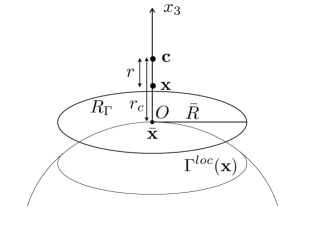
Figure 3: Surface patch ${\Gamma^{loc}(\mathbf{x})}$ and its projection $R_{\Gamma}$ onto the tangent plane at $\bar{\mathbf{x}}$. The expansion center is $\mathbf{c}$, target point is $\mathbf{x}$, and radius of $R_{\Gamma}$ is $\bar{R}$.

Our estimate for the truncation error of the double layer potential is the following:

Theorem 5.1.

Let $E_{T}$ be the truncation error of the local double layer potential $\mathcal{D}_{L}\sigma(\mathbf{x})$ evaluated by Taylor’s expansion of order $p$ about the point $\mathbf{c}=(0,0,c)$. Then under the above assumptions, $E_{T}$ evaluated at a target point $\mathbf{x}=(0,0,x_{3})$ inside the radius of convergence of the Taylor’s series satisfies the bound

$$E_{T}\leq C\ p\ \alpha_{p+1}\left|\sigma({\bf 0})\right|\frac{\left[(1+\sqrt{2})\ r\right]^{p+1}}{\left(\sqrt{c^{2}+{\bar{R}}^{2}}\right)^{p+1}}\left(1+O\left(\frac{c^{2}}{c^{2}+{\bar{R}}^{2}}\right)\right)\\ +O\left(\alpha_{p}\ p\ |\sigma({\bf 0})|\ {\cal H}{\bar{R}}\frac{r^{p+1}}{(\sqrt{c^{2}+{\bar{R}}^{2}})^{p+1}}\right),$$ (39)

where $r=|x_{3}-c|$, ${\cal H}$ is the mean curvature of ${\Gamma^{loc}(\mathbf{x})}$ at $\bar{\mathbf{x}}$, $C$ is a constant, and $\alpha_{p}$ is defined in Lemma 9.3, Appendix C.

The error estimates are chiefly used to assess the order of convergence for different relative orderings of the numerical parameters. We give some examples.

1. In the error expressions (37) and (39), we identify both $|c|$ and the minimum panel-to-center distance $r_{P}$ with $r_{c}$ (cf. (25)), and note that $r\leq r_{c}$. If we place the expansion center a distance $r_{c}=O(h^{1/2})$ from the surface and fix $\bar{R}$, then the truncation error is at most $O(h^{(p+1)/2})$. The dominant term in the coefficient error is $e^{-4qr_{c}/h}$ which is $O(e^{-1/h^{1/2}})$. The third source of error, i.e., the interpolation error from upsampling, is $O(h^{q_{int}})$. All the errors tend to zero, and high order can be achieved by choice of $p$ and $q_{int}$ (cf. Table 2, §7). In this case, the method is classically convergent.

2. We may also desire that the local QBX correction take $O(1)$ work per target as the grid is refined, so that its overall complexity is $O(N)$. This can be achieved by setting $\bar{R}=O(h)$. (Later, we will identify $\bar{R}$ with a numerical ‘distance’ parameter $d_{QBX}$.) The error estimates require that we also set $r_{c}=O(h)$, in which case the coefficient and truncation errors remain fixed, but controllably small, as $N$ increases. The total error then has the form $E=O(\epsilon+h^{q_{int}})$, where $\epsilon$ is the sum of the coefficient and truncation error, and $h^{q_{int}}$ is the interpolation error. In this case, our QBX method is not classically convergent, but converges with controlled precision (cf. Table 3, §7). This type of error is also discussed in [21].

3. Numerical parameters for most of the computational examples in §7 are chosen so that the quadrature and truncation errors are dominated by the $O(h^{q_{int}})$ interpolation error. We make the specific choice $q_{int}=7$.

6 Local QBX algorithm

6.1 On-surface evaluation

We describe in more detail our local QBX computation of the double layer potential in (30), (31). The process is different for target points on the surface, which makes use of a precomputation, then for target points that are nearby but off the surface, for which the QBX correction is computed ‘on the fly.’ We begin with the on-surface evaluation. We want to compute

$$u_{L}(\mathbf{x}_{i})=\mathcal{D}_{L}^{h}\sigma(\mathbf{x}_{i}),\quad i=1,\ldots,N$$ (40)

where $\mathcal{D}_{L}$ was defined in (30), and the superscript $h$ indicates that this is a numerically computed approximation. The target points $\mathbf{x}_{i}\in\partial D$ are the points for which we are enforcing (12),(13).

Let $\mathbf{x}_{i}\in\partial D_{k}$, and assume for now that ${\Gamma^{loc}(\mathbf{x})}$ includes a set of neighboring surface panels on $\partial D_{k}$, but no other parts of $\partial D$. We will call this set of panels the local patch. Denote the total number of discretization points within the local patch by $n_{\mathbf{x}_{i}}$, their locations by $\mathbf{x}_{q},\,q=1,\ldots n_{\mathbf{x}_{i}}$, and let $\mathbf{\Sigma}_{i}\in{{\rm l}\kern-1.49994pt{\rm R}}^{n_{\mathbf{x}_{i}}}$ contain $\{\sigma(\mathbf{x}_{q})\}_{q=1}^{n_{\mathbf{x}_{i}}}$.

Given an expansion center $\mathbf{c}_{i}$ and an expansion order $p$, we can precompute a vector $R_{i}\in{{\rm l}\kern-1.49994pt{\rm R}}^{n_{\mathbf{x}_{i}}}$ such that

$$u_{L}(\mathbf{x}_{i})=R_{i}\cdot\mathbf{\Sigma}_{i}.$$ (41)

The vector $R_{i}$ represents the resulting action after $i)$ upsampling the density $\sigma$ to a finer grid locally on each surface panel (upsampling factor $\kappa$), $ii)$ using the fine grid to compute the expansion coefficients (31) at the expansion center $\mathbf{c}_{i}$ up to order $p$, including only the surface panels in the local patch, and $iii)$ finally evaluating the expansion (30) (summing from $n=0$ to $p$) at $\mathbf{x}_{i}$.

The numbers in $R_{i}$ are the effective quadrature weights. They are however target specific, i.e. for each $\mathbf{x}_{i}$ we will in general find a different set of values. If the surface $\partial D_{k}$ is e.g. axisymmetric, or if there are multiple $D_{k}$’s with the same surface shape, then several target points can use the same $R_{i}$ values. Precomputation was also used in [18] for simulations of Stokes flow with axisymmetric spheroidal particles.

By scaling $n_{\mathbf{x}_{i}}$ to have $O(1)$ size as $N$ is increased, the dot product in (41) has $O(1)$ complexity per target, or a total complexity of $O(N)$ for the evaluation of (41) over all the targets.

The on-surface target points are the discretization points in the regular quadrature for $\partial D_{k}$, $k=1,\ldots,M$. Hence, we know the location of the target points and we precompute and store the vectors $R_{i}$ for all $\mathbf{x}_{i}$ on $\partial D$, $i=1,\ldots,N$. They can then be reused in each GMRES iteration.

By construction, QBX evaluates the one-sided limit of a layer potential as $\mathbf{x}$ approaches the boundary on the side of the expansion center. If this one-sided limit is the quantity of interest, then no further post-processing is needed. However, if the integral ${\cal D}\sigma(\mathbf{x})$ is desired for $\mathbf{x}$ on the boundary $\partial D$, then additional steps are necessary. One option is to add/subtract the relevant quantity from the one-sided limit, as in (5). A second option is to compute both one-sided limits using QBX and average, i.e.,

$${\cal D}\sigma(\mathbf{x})=\frac{1}{2}\left(\lim_{\mathbf{x}\rightarrow\partial D_{+}}{\cal D}\sigma(\mathbf{x})+\lim_{\mathbf{x}\rightarrow\partial D_{-}}{\cal D}\sigma(\mathbf{x})\right)$$

by two applications of QBX. The advantages and disadvantages of these approaches are discussed at length in [21]. Both options were investigated in the numerical examples reported in Section 7, with little or no difference in the results for the specified error tolerances.

6.2 Off-surface target points

Off-surface target points that are close to the surface (the nearly singular case) occur because another surface is close by as we are solving the integral equation for the exterior problem (9), or in the post-processing step when we want to compute the solution anywhere in the domain. If the locations of these target points are not known before hand, target specific quadrature weights cannot be precomputed. In addition, there is a limit to how many precomputed numbers are practical to store.

Hence, these computations are done on the fly, as they are determined to be necessary. For each target point $\mathbf{x}_{i}$, it needs to be determined what panels should be included in ${\Gamma^{loc}(\mathbf{x})}$. This is done efficiently utilizing a tree structure. The density $\sigma$ must then be upsampled to a finer grid locally on each panel such that expansion coefficients can be accurately computed. Here we use an adaptive strategy, where the distance from the patch to the target point will determine the upsampling factor $\kappa$. This will be further discussed in next section, where the full algorithm is discussed.

6.3 The full algorithm

Recall that each boundary component $\partial D_{k}$, $k=1,\ldots,M$ is tiled into $N_{\theta}^{k}\times N_{\varphi}^{k}$ surface panels, with $q^{2}$ Gauss-Legendre points on each, where we use the particular value $q=7$. We solve the second kind integral equation (12) or (13) for the interior or exterior problem, respectively, discretized by a Nyström method with GMRES to find the discrete values of the double layer density $\sigma$. Then for any given point $\mathbf{x}$ in the solution domain, we evaluate (14) or (15) to obtain the solution at that point.

When performing a matrix-vector multiply in a GMRES iteration, or in a post-processing step to find the solution $u$, the double layer potential $\mathcal{D}^{h}\sigma(\mathbf{x})$ must be computed. In the previous sections, we have described how the direct quadrature is not sufficient when the evaluation point $\mathbf{x}$ is either close to a boundary component, introducing a nearly singular integral, or actually on a boundary surface (singular integral). The on-surface treatment is done with QBX and was discussed in Section 6.1. The QBX evaluation for off-surface target points was discussed in Section 6.2. However, upsampling of panels can be sufficient by itself if the evaluation (target) point is not too close to the surface.

Denote by $d_{P}(\mathbf{x}_{i})$ the closest distance from target point $\mathbf{x}_{i}$ to panel $P$. Assume that we are given two distances $d_{up}$ and $d_{QBX}$ such that if $d_{P}(\mathbf{x}_{i})>d_{up}$, the direct quadrature on the original grid is sufficient, if $d_{QBX}<d_{P}(\mathbf{x}_{i})\leq d_{up}$ we want to use upsampling of the panel, and for $d_{P}(\mathbf{x}_{i})\leq d_{QBX}$ we will use the QBX treatment. Figure 4 provides an illustration.

The algorithm for evaluating $\mathcal{D}^{h}\sigma(\mathbf{x})$ then starts by evaluating $\mathcal{D}^{h}\sigma(\mathbf{x})$ with the direct (coarse grid) quadrature at all target points using a fast hierarchical algorithm (here we use the treecode algorithm in [25]). The incorporation of an FMM or treecode is therefore entirely standard, and a ‘black box’ algorithm can be used. However, this quadrature will not be accurate for panels that are close to each target point $\mathbf{x}_{i}$, and a local correction must then be done. We start by finding all panels P with $d_{P}(\mathbf{x}_{i})\leq d_{up}$ (using a tree structure), and for each panel in the set we subtract off the contribution based on the direct quadrature over that panel, $Q^{P}_{q}[\sigma K(\mathbf{x}_{i},.)]$, and subsequently add on a more accurate quadrature as described below.

Then as depicted in Figure 4:

• If $\mathbf{x}_{i}\in\partial D_{k}$ for some $k$, evaluate the QBX contribution from all panels in the local patch $\Gamma^{loc}(\mathbf{x}_{i})$ that are on the same surface component as $\mathbf{x}_{i}$, using the precomputed target specific weights (41).

• For all other panels such that $d_{QBX}<d_{P}\leq d_{up}$, add upsampled quadrature contribution $Q^{P}_{q,\kappa}[\sigma K(\mathbf{x}_{i},.)]$ (see (18)).

• For all panels in $\Gamma^{loc}(\mathbf{x}_{i})$ not yet included, pick a center $\mathbf{c}_{i}$ associated with $\mathbf{x}_{i}$ and evaluate the contributions to the QBX coefficients $z^{L,h}_{n}(\mathbf{x}_{i})$, $n=0,\ldots,p$, using upsampled quadrature (here we use with $q=15$). Form the sum (33) to evaluate the QBX expansion at $\mathbf{x}_{i}$.

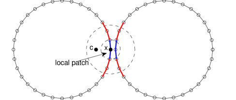
Figure 4: Computation of the local QBX correction at $\mathbf{x}$ using center $\mathbf{c}$. ${\cal D}_{L}^{h}\sigma(\mathbf{x})$ is computed over blue panels using QBX, and over red panels by direct upsampled quadrature. Spheres of radius $d_{up}$ and $d_{QBX}$ (with $d_{up}>d_{QBX}$) are shown.

There are several parameters that need to be set. Assume that the underlying discretization has been set, with a total of $N_{p}$ panels and $q^{2}$ quadrature points on each, such that $N=N_{P}\times q^{2}$. If the error saturates as we increase $d_{up}$, $d_{QBX}$, upsampling factors and expansion order $p$ for our quadrature method, we are seeing the error of the underlying discretization. Hence, if a smaller error is needed, $N$ must then be increased.

Now assume that we have a fine enough underlying discretization, and that we wish to set a tolerance for the relative quadrature error, and select the parameters for the quadrature method thereafter. Hence, we need to set $d_{up}$, $d_{QBX}$, $p$, $r_{c}$ (or a way to select the center $\mathbf{c}_{i}$ given a target $\mathbf{x}_{i}$), and we also need to set the upsampling rates, both for the direct upsampling as described below, and for the quadrature when computing the QBX coefficients.

At this point, we do not have explicit expressions for exactly how to set these parameters, although the estimates for the truncation and coefficient errors given in Section 5 guide our choice. In those error expressions (see (37) and (39)), we identify $\bar{R}$ with the parameter $d_{QBX}$, $r$ with the center-to-target distance $|c_{i}-\mathbf{x}_{i}|$, and as noted earlier both $|c|$ and the (minimum) panel-to-center distance $r_{P}$ with $r_{c}$ (cf. (25)). We typically choose $d_{QBX}$ and the center position $\mathbf{c}_{i}$ as described below so that $d_{QBX}$, $r$, and $r_{c}$ are proportional to the panel size $h$. As discussed in Example 3, Section 5, this has the effect of fixing the coefficient and truncation error at a small value as $h$ is reduced. Crucially, this scaling of parameters with $h$ also leads to the desired $O(1)$ work per target in the local correction step.

In the next section, we introduce the evaluation of the double layer potential over the unit sphere with the density $\sigma$ set as a spherical harmonic function $Y_{n}^{m}$. For this case, we have an analytical solution both for on-surface and off-surface target points. We will use this example to set our parameters.

We will first discuss how to set the parameters for the on-surface evaluation (Section 6.1). In $i)$ above, we have assumed that the target specific weights resulting from the QBX procedure have been precomputed, as we would do when we want to solve an integral equation. They could also of course be computed directly with the same parameter choices.

Now, let $\bar{h}$ denote a typical panel dimension. Given a collection of on-surface target points $\mathbf{x}_{i}$, $i=1,\ldots,N_{set}$, define the local patch for each target by the set of the surface panels for which the closest distance from $\mathbf{x}_{i}$ to the panel is less than $\bar{h}$. Then do the following:

• Set the expansion radius $r_{c}$ no larger than $\bar{h}/2$. The center $\mathbf{c}_{i}$ will then be set at a distance $r_{c}$ from the surface normally out from $\mathbf{x}_{i}$. Note that for the on-surface evaluation, $r=r_{c}$. We also set $d_{QBX}=r_{c}$, or a small multiple of it.

• Set a large upsampling ratio $\kappa$ for all panels in the local patch, and increase $p$ until the desired accuracy is reached for all targets. That sets the value of $p$.

• Now, with $r_{c}$ and $p$ selected, start to reduce $\kappa$. Pick the smallest value possible before it adversely starts to affect your accuracy.

• Adaptive reduction of $\kappa$. The minimum distance from the closest panel to the expansion center is $r_{c}$. Assume that the closest distance from panel $P$ is $r_{P}$. According to the error estimate for the coefficient error, the contribution of the error from panel $P$ will be comparable to the one from the closest panel if $\kappa_{P}r_{P}=\kappa r_{c}$, where $\kappa_{P}$ is the upsampling ratio for panel $P$. Hence, depending on the size of $r_{P}$, $\kappa$ could possibly be reduced (always to an integer value). This type of adaptive reduction is described in [21], and a similar version has been implemented here for the off-surface QBX evaluation.

We will now discuss the off-surface evaluation, starting with the standard upsampling. It is easy to test for off-surface points and find the limit $d_{up}$ up to which distance, but no closer, the direct quadrature is sufficiently accurate. According to the error estimate (37), if the upsampling ratio is doubled, the same accuracy can be retained for targets a distance $d_{up}/2$ from the surface. This gives a recipe to choose $\kappa$ at different distances. To keep it simple, we however take $\kappa$ in the whole upsampling region to be the $\kappa$ needed at the distance $d_{QBX}$. If the distance is smaller than $d_{QBX}$, we will switch to the QBX evaluation.

The off-surface QBX evaluation will use the value of $r_{c}$ and the number of expansion terms $p$ selected in the on-surface procedure. Here however, if a target point is at a distance $\tilde{r}_{c}$ from the surface, the center will be placed in the (approximately) normal direction, another distance $r_{c}$ away, yielding a distance from the center to the surface of approximately $\tilde{r}_{c}+r_{c}$. The integrals to evaluate for the QBX coefficients will hence typically require less resolution than for the on-surface evaluation (since they are not as nearly singular), but for target points extremely close to the surface, it will be essentially the same, and we will keep the same parameters as for the on-surface evaluation.

7 Validation/Numerical results

In this section, we illustrate the performance of the target specific QBX method in several examples. Table 1 reviews the main numerical parameters. Other than $d_{up}$, which is fixed at $2\cdot d_{QBX}$, the specific values of the parameters are given in each example below.

$N_{\theta}(=N_{\phi})$	no. panels on each $\partial D_{k}$ is $N_{\theta}\times N_{\phi}$	§3
$d_{QBX}$	QBX criteria $0<d_{P}(\mathbf{x})\leq d_{QBX}$	§6.3
$d_{up}(=2d_{QBX})$	direct upsampling criteria $d_{QBX}<d_{P}(\mathbf{x})\leq d_{up}$	§6.3
$\kappa$	upsampling factor	§3.1
$r_{c}$	minimum distance from expansion center to surface	§4, eq. (25)
$p$	truncation level	§4.2, eq. (33)

Table 1: Main numerical parameters, and the section where each is introduced. Here $d_{P}(\mathbf{x})$ is the minimum distance from the target point $\mathbf{x}$ to panel $P$.

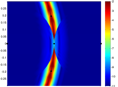
Figure 5: $l^{\infty}$ error in the potential ${\cal D}Y_{2}^{2}$ computed using 15 point Gauss-Legendre quadrature over $32^{2}$ panels, except in two small spheres $|\mathbf{x}-\mathbf{c}_{\pm}|\leq r_{c}$ centered at off-surface points $\mathbf{c}_{\pm}$ on either side of $\partial D$ a distance $r_{c}=0.3$ from the boundary. The potential in the spheres is computed using our local QBX method with parameters $N_{\theta}=16,\kappa=2,$ and $d_{QBX}=0.7$ Only a small portion of the boundary $\partial D$ is shown. The markers indicate the panel size and locations of $\mathbf{c}^{\pm}$.

7.1 Evaluation of layer potentials

We first validate our numerical method in calculations involving a single sphere using exact analytical formulae for eigenfunctions of the double layer potential and separation of variable solutions for the interior and exterior Dirichlet problems. For $D$ a unit sphere, it is straightforward to show that

$$\int_{\partial D}Y_{l}^{m}(\theta^{\prime},\phi^{\prime})\frac{\partial G(\mathbf{x}(\theta,\phi),\mathbf{y}(\theta^{\prime},\phi^{\prime}))}{\partial\nu(\mathbf{y}(\theta^{\prime},\phi^{\prime}))}W(\theta^{\prime},\phi^{\prime})~{}d\theta^{\prime}d\phi^{\prime}=-\frac{Y_{l}^{m}(\theta,\phi)}{4l+2},$$ (42)

i.e., the spherical harmonic function $Y_{l}^{m}$ is an eigenfunction of the double layer potential with eigenvalue $-(4l+2)^{-1}$. Furthermore, substituting $\sigma(\theta,\phi)=Y_{l}^{m}(\theta,\phi)$ into (5) and comparing with the separation of variables solution in spherical coordinates, we see that

$$u(\rho,\theta,\phi)={\cal D}Y_{l}^{m}(\rho,\theta,\phi)=\left\{\begin{array}[]{ll}&-\frac{l+1}{2l+1}\ \rho^{l}Y_{l}^{m}(\theta,\phi)~{}~{}\mbox{for}~{}~{}|\rho|<1,\\ &\frac{l}{2l+1}\ \rho^{-(l+1)}Y_{l}^{m}(\theta,\phi)~{}~{}\mbox{for}~{}~{}|\rho|>1,\end{array}\right.$$ (43)

is the solution to the interior and exterior Dirichlet problems with boundary data given by the respective solution in (43) evaluated at $\rho=1$.

Figure 5 provides an illustrative example of our method, by superimposing the errors from a QBX calculation of the double layer potential in an interior and exterior spherical region on top of an error plot from a computation of the potential using a standard Gauss-Legendre quadrature. The error in ${\cal D}\sigma$ computed by the QBX expansion is much smaller than the error of the standard computation throughout both spherical regions. These two regions are where the expansions about the centers $\mathbf{c}_{\pm}$ converge; it is here that the QBX method corrects the inaccuracies of the standard quadrature.

Our next example (Table 2) relates the error estimates in Section 5 to numerical results. We compute the double layer potential on the surface of the unit sphere using the eigenfunction density $\sigma=Y_{2}^{2}$, and compare with the analytical result (42). In the top two sets of entries, for $p=3$ and $7$, the distance of the expansion center from the interface is scaled as $r_{c}=O(h^{1/2}$). This is the scaling discussed in Example 1 of Section 5, for which the sum of the coefficient and truncation errors is $O(h^{(p+1)/2})$. Thus, the analysis predicts a second order method for $p=3$ and a fourth order method for $p=7$, and this is approximately observed in practice. The third set of entries is a high accuracy computation with $p=20$ and fixed $r_{c}$. In this example, the truncation and coefficient errors are small enough that the the total error is dominated by the interpolation of the density, which is $O(h^{q_{int}})$ with $q_{int}=7$. The numerical results are roughly consistent with this expected order of accuracy. Here and below, $h$ refers to the length of one side of a Gauss-Legendre panel in $(\theta,\phi)$; more precisely, the panel dimensions are $h\times 2h$ since we use the same number of panels in $\theta$ and $\phi$. In all subsequent examples, parameters are chosen so that the $O(h^{q_{int}})$ interpolation error is the dominant source of error.

$p$	$N_{\theta}(=N_{\phi})$	$r_{c}$	$l^{2}$ error	$l^{\infty}$ error	EOC
$3$	$4$	$0.2$	$3.1\times 10^{-2}$	$4.8\times 10^{-2}$	$-$
	$8$	$0.15$	$1.1\times 10^{-2}$	$1.2\times 10^{-2}$	$2.0$
	$16$	$0.1$	$1.9\times 10^{-3}$	$1.5\times 10^{-3}$	$3.0$
	$32$	$0.075$	$2.1\times 10^{-4}$	$3.0\times 10^{-4}$	$2.2$
$7$	$4$	$0.2$	$1.1\times 10^{-2}$	$1.2\times 10^{-2}$	$-$
	$8$	$0.15$	$3.2\times 10^{-4}$	$3.9\times 10^{-4}$	$4.9$
	$16$	$0.1$	$2.3\times 10^{-5}$	$1.6\times 10^{-5}$	$4.6$
	$32$	$0.075$	$3.8\times 10^{-7}$	$5.5\times 10^{-7}$	$4.8$
$20$	$4$	$0.2$	$1.8\times 10^{-5}$	$2.8\times 10^{-5}$	$-$
	$8$	$0.2$	$4.3\times 10^{-7}$	$5.7\times 10^{-7}$	$5.4$
	$16$	$0.2$	$5.8\times 10^{-9}$	$8.0\times 10^{-9}$	$6.2$
	$32$	$0.2$	$1.5\times 10^{-11}$	$2.5\times 10^{-11}$	$8.6$

Table 2: Relative $l^{2}$ and $l^{\infty}$ error in the computation of the on-surface double layer potential ${\cal D}Y_{2}^{2}$. EOC is the empirical order of convergence calculated using the $l^{2}$ error at the previous level of grid refinement. Other parameter values are $\kappa=2,d_{QBX}=0.35$ for $p=3,~{}7$ and $\kappa=8,d_{QBX}=0.7$ for $p=20$.

Figure 6 shows how the relative $l^{\infty}$ error varies with $p$ for the computation of the on-surface double layer potential ${\cal D}Y_{2}^{2}$ in Table 2. At small values of $p$ the curves for different resolution $N_{\theta}$ overlap, indicating that the error is dominated by the truncation error. For larger $p$ the interpolation error dominates, and thus the higher resolution computations are more accurate. The error estimates discussed in Section 5 suggest that the coefficient error grows with $p$ and can become dominant at sufficiently large $p$ when other parameters are held fixed. This is observed in the lowest resolution ($N_{\theta}=4$) curve, but is not seen in this $p$ range for the higher resolution computations.

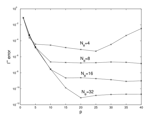
Figure 6: Relative $l^{\infty}$ error versus truncation $p$ in the computation of the on-surface double layer potential ${\cal D}Y_{2}^{2}$. Parameter values are $\kappa=8,~{}r_{c}=0.2,~{}d_{QBX}=0.7$.

Table 3 shows the same calculation of the on-surface double layer potential ${\cal D}Y_{2}^{2}$ as in Table 2 when $p=20$, but instead of fixing the cut-off parameter $d_{QBX}$ (as is done there) we now vary it with the scaling $d_{QBX}\sim r_{c}\sim h$ (cf. §5). In this and all subsequent computations using this scaling, we employ an upsampling layer with $d_{up}=2\ d_{QBX}$ and a factor $\kappa=2$. With these parameter scalings, the truncation and coefficient errors are fixed as the number of panels is increased. The parameter values are chosen so that these errors are negligible and the dominant source of error is the $O(h^{7})$ interpolation error. This is consistent with the data in Table 3.

$N_{\theta}(=N_{\phi})$	$d_{QBX}$	$r_{c}$	$l^{2}$ error	$l^{\infty}$ error	no. ops.	ops. ratio	EOC
$2$	$1.4$	$0.4$	$5.6\times 10^{-4}$	$6.0\times 10^{-4}$	$3.5\times 10^{4}$	$~{}~{}~{}~{}-$	$~{}~{}-$
$4$	$0.7$	$0.2$	$1.3\times 10^{-5}$	$1.3\times 10^{-5}$	$2.0\times 10^{5}$	5.7	5.5
$8$	$0.35$	$0.1$	$2.7\times 10^{-7}$	$1.8\times 10^{-7}$	$9.7\times 10^{5}$	4.9	5.6
$16$	$0.17$	$0.05$	$2.5\times 10^{-9}$	$1.53\times 10^{-9}$	$4.5\times 10^{6}$	4.6	6.8

Table 3: Relative $l^{2}$ and $l^{\infty}$ error in the computation of the on-surface double layer potential ${\cal D}Y_{2}^{2}$. The cut-off parameter $d_{QBX}$ and distance of the centers from the boundary $r_{c}$ are scaled as $d_{QBX}\sim r_{c}\sim h$. Parameter values are $\kappa=16$, $p=30$ for the QBX region, and $d_{up}=2\cdot d_{QBX}$, $\kappa=2$ for the local upsampling region. The number of operations in the dot product of the local QBX correction (41) is shown, as is the ratio of two of these values for $N_{\theta}$ and $2\cdot N_{\theta}$ panels.

The parameter scaling in Table 3 has the additional benefit of conferring an $O(N)$ complexity on the local QBX correction over all targets. To verify this, we show in the table the number of operations in the local QBX computation (41) over all targets, as well as the ratio of operations for $N_{\theta}$ and $2\cdot N_{\theta}$ panels. In principle this ratio should be $4$, since the number of targets increases by a factor of $4$ when $N_{\theta}=N_{\phi}$ is doubled. The observed ratio is not exactly $4$, due to the discrete (and nonuniform) panel sizes in physical space, but approaches $4$ asymptotically in $N_{\theta}$.

We turn now to computation of the double layer potential at targets points that are off, but close to, the surface. Figure 7 show an example calculation of the relative error in the off-surface computation of the double layer potential ${\cal D}\sigma$ using the same source density $\sigma=Y_{2}^{2}$. In the figure we evaluate the potential at a set of targets along the $x$-axis, i.e., at $\theta=\pi/2$, $\phi=0$ just outside the sphere. The figure compares computations using our QBX method with those using a local upsampling method in which the local correction (i.e., the correction to the double layer integral for source points close to the target) is computed directly, without any local expansion, using oversampled 15-point Gauss-Legendre quadrature. The two methods agree far enough away from the sphere, but the upsampling method starts to lose accuracy when the target point is about $4$ to $5$ grid points away from the boundary (based on the upsampled grid spacing). Sufficiently close to the boundary the error using upsampling alone is $O(1)$, regardless of the fineness of the grid. In contrast, the QBX method maintains accuracy all the way up to the boundary.

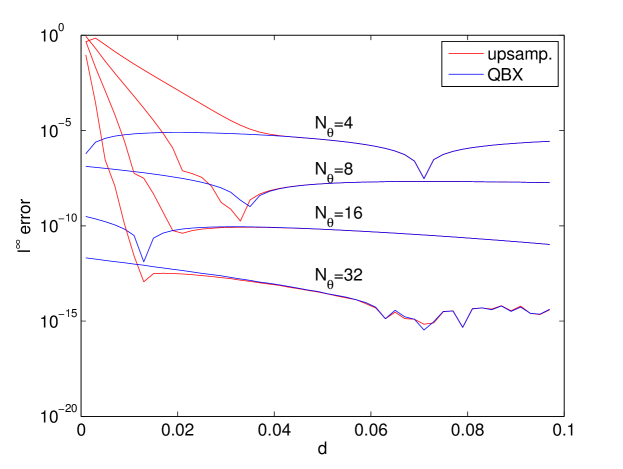
Figure 7: Comparison of relative $l^{\infty}$ error using the QBX method and a local upsampling method to compute ${\cal D}Y_{2}^{2}$ at a target point a distance $d$ from the surface of the unit sphere. The different curves correspond to different numbers of panels $N_{\theta}(=N_{\phi})$. Parameter values are as in Table 2 ($p=20$). The oversampling factor for the local upsampling method is $\kappa=8$.

7.2 Solution of the integral equation for different domains

7.2.1 Single sphere

A more involved test case is to solve the second kind integral equation (9) or (10) that arises in the Green’s function formulation of the Dirichlet problem. We use a Nyström method where the unknowns are the point values of the density $\sigma$ at the target nodes, and employ GMRES to solve the discrete equations (12) or (13) iteratively. At each iteration, the double layer potential is computed via the target-specific QBX method with precomputation. Except where noted, we set the GMRES tolerance to $10^{-10}$. After solving for $\sigma$, we use the double layer representation to evaluate the potential $u$ at a collection of target points.

As a first example, we specify boundary data on the unit sphere to be that generated by an exact solution from (43), and then compute the solution to the interior/exterior Dirichlet problem. The error in the computed solution can be assessed by comparison with the analytical solution. The results of some example computations are shown in Table 4. The magnitude of the errors are similar to those in the calculation of layer potentials alone. Note the number of iterations in the GMRES calculation typically decreases as the number of panels is increased, which is also observed in our other numerical tests.

side	$N_{\theta}(=N_{\phi})$	target $r_{*}$	$l^{2}$ error	$l^{\infty}$ error	its.
int	$4$	$\sigma$	$3.5\times 10^{-6}$	$5.0\times 10^{-6}$	7
		0.99	$6.6\times 10^{-6}$	$5.4\times 10^{-6}$
		0.5	$7.1\times 10^{-7}$	$2.9\times 10^{-7}$
	$8$	$\sigma$	$8.5\times 10^{-8}$	$1.0\times 10^{-7}$	11
		0.99	$4.5\times 10^{-8}$	$4.9\times 10^{-8}$
		0.5	$2.6\times 10^{-8}$	$1.3\times 10^{-8}$
	$16$	$\sigma$	$2.7\times 10^{-9}$	$3.5\times 10^{-9}$	4
		0.99	$4.2\times 10^{-10}$	$2.7\times 10^{-10}$
		0.5	$5.1\times 10^{-11}$	$2.4\times 10^{-11}$
ext	$4$	$\sigma$	$4.1\times 10^{-6}$	$6.2\times 10^{-6}$	6
		1.01	$7.9\times 10^{-6}$	$7.1\times 10^{-6}$
		1.5	$2.7\times 10^{-6}$	$9.9\times 10^{-7}$
	$8$	$\sigma$	$3.2\times 10^{-8}$	$7.3\times 10^{-8}$	5
		1.01	$1.7\times 10^{-7}$	$2.2\times 10^{-7}$
		1.5	$4.4\times 10^{-8}$	$2.7\times 10^{-8}$
	$16$	$\sigma$	$8.8\times 10^{-10}$	$1.1\times 10^{-9}$	3
		1.01	$1.6\times 10^{-9}$	$8.9\times 10^{-10}$
		1.5	$1.1\times 10^{-10}$	$5.5\times 10^{-11}$

Table 4: Errors in evaluating the solution to an interior/exterior Dirichlet problem at a set of targets on a sphere of radius $r_{*}$, via solving a second kind integral equation for the density $\sigma$. Boundary data is given by (43) with $l=m=2$ and $\rho=1$. A $\sigma$ in the $r_{*}$ column denotes that the errors are listed for $\sigma$. GMRES iteration counts are shown in the last column. Fixed parameter values are $\kappa=8,p=20,r_{c}=0.2,d_{QBX}=0.7$.

Another test of our method is shown in Table 5. For an exterior boundary value problem, we now generate an exact solution to Laplace’s equation by introducing a collection of point charges in the interior region. This exact solution is then used to provide Dirichlet data for our boundary value problem, which is solved using an integral equation. We test the accuracy of our solution at a collection of target points on a sphere of radius $r_{*}$ surrounding the domain $D$.

The results of this exterior calculation are shown in Table 5. For both of the examples in Tables 4 and 5, the error in solving the integral equation and evaluating the solution near the surface $\partial D$ is roughly the same order of magnitude as the error in evaluating the double layer potential alone (cf. Tables 2 and 3). We note that accuracy is maintained at a similar level when the target $r_{*}$ is even closer to $1$. This shows that the method can compute within a specified accuracy for target points that are arbitrarily close to the domain boundary.

side	$N_{\theta}(=N_{\phi})$	target $r_{*}$	$l^{2}$ error	$l^{\infty}$ error	its.
ext	$4$	$1.005$	$1.4\times 10^{-5}$	$1.9\times 10^{-5}$	10
		1.5	$2.8\times 10^{-6}$	$1.9\times 10^{-6}$
	$8$	$1.005$	$6.2\times 10^{-7}$	$8.0\times 10^{-7}$	9
		1.5	$8.9\times 10^{-8}$	$5.4\times 10^{-8}$
	$16$	$1.005$	$5.8\times 10^{-9}$	$7.2\times 10^{-9}$	8
		1.5	$1.5\times 10^{-10}$	$8.8\times 10^{-11}$

Table 5: Accuracy of exterior Dirichlet computation for a domain with a single sphere, when boundary data is generated by $49$ point charges spread around a spherical interior surface with radius $\rho=0.5$. Errors are evaluated at a set of targets on a sphere of radius $r_{*}$. Other parameter values are as in Table 4.

7.2.2 Nonspherical shape

Table 6 illustrates the accuracy of our method for some example nonspherical geometries. In (a) we consider a triaxial ellipsoid with semi-major axes lengths $1/2,1$, and $2$. In (b) we choose a shape with four-fold symmetry in the $\phi$-direction, whose boundary is described by $\mathbf{x}(\theta,\phi)=\rho_{s}(\theta,\phi){\boldsymbol{\omega}}(\theta,\phi)$ where $\rho_{s}(\theta,\phi)=1+\varepsilon\sin^{2}\theta\cos 4\phi$ and ${\boldsymbol{\omega}}(\theta,\phi)$ is the standard spherical-coordinate parameterization of a unit sphere, and we take $\varepsilon=0.3$. This form satisfies the requirement that $\rho_{s}$ is independent of $\phi$ at $\theta=0,\pi$ and that $\partial_{\theta}\rho_{s}(\theta=0,\phi)=\partial_{\theta}\rho_{s}(\theta=\pi,\phi)=0$, which is necessary for smoothness of the surface shape at the poles. We introduce a collection of unit point charges in the interior of each shape, spread over a spherical surface of radius $\rho=0.2$, and use the point charges to generate boundary data for the exterior problem. The boundary shapes and interior point charges are shown in Figure 8.

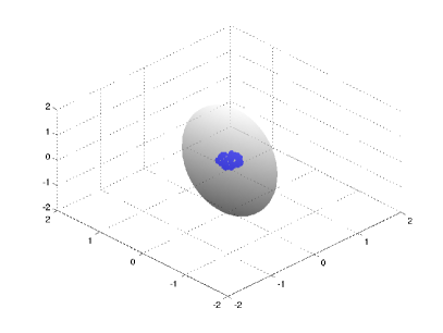
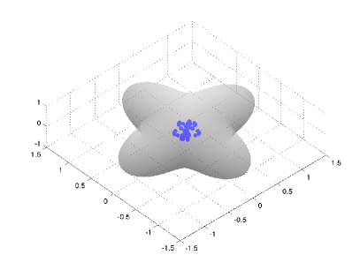
Figure 8: Boundary shapes and point charges for the tests of the solution to the exterior Dirichlet problem in Table 6. Left: Triaxial ellipsoid, right: four-fold symmetry.

In these examples, we employ the same scaling of parameters as in Table 3; namely $d_{QBX}\sim r_{c}\sim h$. The support of the region where the local QBX correction is made then shrinks for each increase in $N_{\theta}$, which gives a storage and computation cost of $O(1)$ per target.

The results are shown in Table 6. The decrease in error with $N_{\theta}$ for the triaxial ellipsoid is roughly similar to that which is observed for a spherical shape. For the four-fold symmetric shape, the error does not decay as rapidly with $N_{\theta}$. This is possibly due to the presence of both positive and negative signed curvature along the surface.

(a) Triaxial ellipsoid

$N_{\theta}(=N_{\phi})$	$\mbox{target}~{}r_{*}$	$d_{QBX}$	$r_{c}$	$l^{2}$ error	$l^{\infty}$ error	its.
$2$	$1.005$	$0.7$	$0.2$	$2.9\times 10^{-4}$	$1.4\times 10^{-3}$	16
	$2.5$			$9.7\times 10^{-5}$	$1.0\times 10^{-4}$
$4$	$1.005$	$0.7$	$0.2$	$3.3\times 10^{-6}$	$4.6\times 10^{-6}$	18
	$2.5$			$1.9\times 10^{-6}$	$2.9\times 10^{-6}$
$8$	$1.005$	$0.35$	$0.1$	$1.7\times 10^{-7}$	$1.9\times 10^{-7}$	17
	$2.5$			$3.8\times 10^{-9}$	$1.2\times 10^{-8}$
$16$	$1.005$	$0.17$	$0.05$	$4.0\times 10^{-9}$	$5.2\times 10^{-9}$	16
	$2.5$			$4.0\times 10^{-11}$	$5.9\times 10^{-11}$

(b) Four-fold symmetric shape $N_{\theta}(=N_{\phi})$ $\mbox{target}~{}r_{*}$ $d_{QBX}$ $r_{c}$ $l^{2}$ error $l^{\infty}$ error its. $2$ $1.005$ $1.4$ $0.4$ $9.4\times 10^{-2}$ $6.8\times 10^{-2}$ 17 $1.8$ $7.5\times 10^{-2}$ $5.1\times 10^{-2}$ $4$ $1.005$ $0.7$ $0.2$ $3.3\times 10^{-5}$ $3.2\times 10^{-5}$ 17 $1.8$ $8.1\times 10^{-5}$ $5.6\times 10^{-5}$ $8$ $1.005$ $0.35$ $0.1$ $2.0\times 10^{-6}$ $3.1\times 10^{-6}$ 17 $1.8$ $4.3\times 10^{-7}$ $3.2\times 10^{-7}$ $16$ $1.005$ $0.17$ $0.05$ $9.4\times 10^{-8}$ $7.9\times 10^{-8}$ 16 $1.8$ $3.5\times 10^{-10}$ $2.3\times 10^{-10}$

Table 6: Accuracy of exterior Dirichlet computation for nonspherical domains. Boundary data is generated by $49$ point charges spread on an interior spherical surface of radius $\rho=0.2$. Errors are evaluated at a set of targets on a larger surrounding surface of the same shape, but scaled by 1.005, and on a spherical surface of radius $r_{*}=2.5$ in (a) and $r_{*}=1.8$ in (b). Other parameters values are as in Table 3.

7.3 Two spheres close to touching

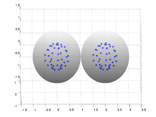
Figure 9: Boundary locations and point charges for the test of the solution in Table 7. The solution is evaluated at a set of targets on a spherical surface that surrounds $D_{1}$ and bisects the gap between the two spheres.

An example using the full target-specific QBX algorithm to solve an exterior Dirichlet problem for two nearly touching spheres is given in Table 7. Let $D_{1}$ and $D_{2}$ denote the two spherical regions, each with unit radius. We introduce point sources inside $D_{1}$ and $D_{2}$ at a radius $\rho=0.5$ with respect to each region’s center to generate boundary data. After solving the integral equation for the density $\sigma$, we evaluate the solution $u(\mathbf{x})$ at a collection of targets located on a spherical surface that surrounds $D_{1}$. The radius $r_{*}$ of the target surface is chosen to bisect the gap between $D_{1}$ and $D_{2}$. This is a challenging test case for our method.

side	$N_{\theta}(=N_{\phi})$	target $r_{*}$	$l^{2}$ error	$l^{\infty}$ error	its.
ext	$2$	$1.005$	$7.1\times 10^{-4}$	$5.5\times 10^{-4}$	31
	$4$	$1.005$	$6.6\times 10^{-6}$	$1.1\times 10^{-5}$	34
	$8$	$1.005$	$2.1\times 10^{-7}$	$3.1\times 10^{-7}$	27
	$16$	$1.005$	$1.7\times 10^{-9}$	$1.3\times 10^{-9}$	25

Table 7: Accuracy of exterior Dirichlet computation for a domain with two unit spheres, with centers a distance $d=2.01$ apart. Boundary data is generated by $49$ point charges located on a spherical surface inside each sphere with radius $r_{p}=0.5$. Errors are evaluated at a set of targets on a sphere of radius $r_{*}$ surrounding $D_{1}$. The number of panels $N_{\theta}$ is per sphere. Other parameter values are as in Table 3.

The error shows good convergence as the number of panels is increased. This demonstrates the accuracy of our method in computing solutions to boundary value problems for closely spaced surfaces.

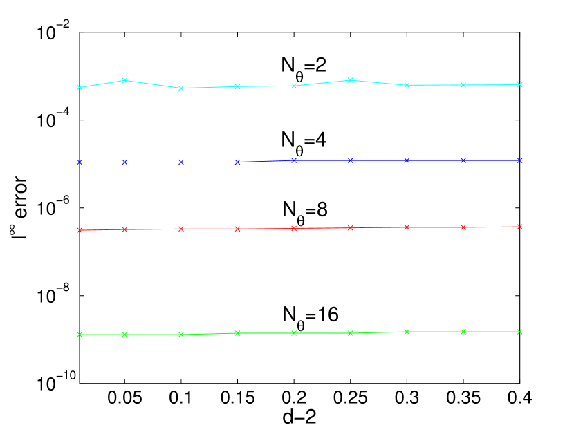
(a) $l^{\infty}$ error for the exterior Dirichlet computation with two unit spheres versus surface separation distance $d-2$. Boundary data, parameter values, and computation of error are as in Table 7.

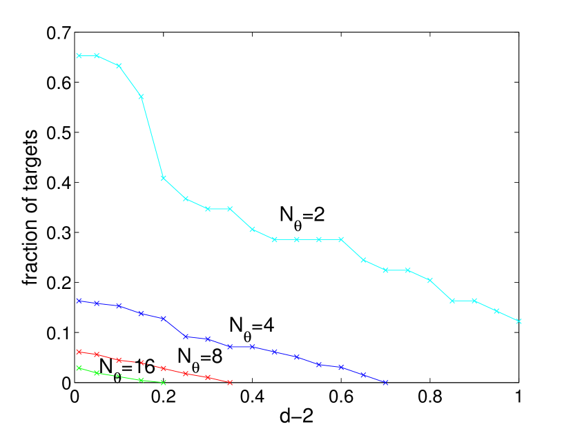
(b) Fraction of targets for which the on-the-fly local QBX correction is made, versus center separation distance $d$, for the two-sphere example in Table 7. Parameter values are the same as in Figure 7.

Figure 10: Effect of separation distance for two sphere problem

Figure 10(a) shows the $l^{\infty}$ error for the two-sphere calculation in Figure 9 as the surface separation distance $d$ is varied. The error is found to be uniform in the separation distance.

We comment on the efficiency of our method for nearly touching particles. When performing the on-surface computation for a single particle, or for multiple particles which are well-separated, there is no need to make the on-the-fly local QBX correction for the interaction of target and source points that lie on different particle surfaces. In this case, all of the local QBX corrections are for the interaction of target/source points that lie on the same surface. These can be precomputed, and the efficiency of the full method is about the same as for computing the global integral using the original grid.

In the computation for two nearly touching particles, however, the on-the-fly local QBX correction is made for target points on each particle that are near the other particle’s surface. Figure 10(b) shows the fraction of target points for which the on-the-fly local correction is made in the two-sphere example in Table 7, plotted versus separation distance $d$. At higher resolutions, the fraction of targets that require the local QBX correction decreases. This is because of the decrease in $d_{QBX}$ with increasing resolution. Thus, the fraction of CPU time spent making the on-the-fly local correction becomes negligible as resolution is increased. The fraction of corrected targets also decreases with increasing separation $d$, as expected.

7.4 A larger problem

Figure 11: Configuration of 40 spheres of unit radius for the exterior Dirichlet computation in Table 8. The distance between spheres is $0.01$.

No.  spheres	$l^{2}$ error	$l^{\infty}$ error	Its.
$4$	$2.0\times 10^{-5}$	$8.3\times 10^{-6}$	$45$
$10$	$6.8\times 10^{-5}$	$2.2\times 10^{-5}$	$66$
$20$	$3.6\times 10^{-6}$	$5.6\times 10^{-6}$	$96$
$30$	$3.7\times 10^{-6}$	$5.7\times 10^{-6}$	$154$
$40$	$2.5\times 10^{-5}$	$8.3\times 10^{-6}$	$267^{*}$

Table 8: Accuracy of exterior Dirichlet computation for multiple unit spheres. The number of panels is fixed at $N_{\theta}(=N_{\phi})=4$ per sphere, with other parameters as in Table 3. Generation of boundary data and location of target surface are as in Table 7. The asterisk denotes that the GMRES tolerance was raised from $10^{-10}$ to $10^{-8}$ for the computation with $40$ spheres.

Our last example considers the exterior Dirichlet problem for a domain with a larger number of unit spheres. We now fix the number of panels per sphere at $N_{\theta}(=N_{\phi})=4$, but vary the number of particles in the domain. For simplicity, the particles are arranged in a simple linear configuration (see figure 10(b)), with the distance between spheres fixed at $0.01$. The boundary Dirichlet data is generated in the same way as for the two-sphere example, i.e., by introducing point sources inside each sphere.

Here we use a treecode, the implementation of which closely follows [25], to compute the global double layer integral. The treecode algorithm divides interface points into a nested set of clusters and approximates velocity interactions between a point and a distant cluster using Taylor’s expansion. Interaction of nearby points is computed using direct summation. The treecode algorithm introduces two additional parameters, the order of the Taylor’s series expansion $p_{T}$, and a separation parameter $\epsilon_{T}$. For the particle-cluster interaction, the Taylor’s approximation is chosen over the direct sum when $\epsilon_{T}>R_{T}/D_{T}$, where $R_{T}$ is the radius of the cluster and $D_{T}$ is the distance from the target point to the cluster center. A decrease in $\epsilon_{T}$ improves the accuracy of the treecode, but slows the computations. Our computations use $\epsilon_{T}=0.2$ and $p_{T}=5$. For a small number of spheres, these values were found to give results that are indistinguishable from direct summation, for the selected number of panels.

The results of our computations are shown in Table 8. The observed accuracy, which is limited by the discretization error, is found to be roughly independent of the number of spheres, but the number of GMRES iterations grows due to ill-conditioning. In [18], a similar behavior is observed as the number of spheroidal particles grows, and the problem is alleviated by introducing a block diagonal preconditioner.

7.5 Operation count for TSQBX versus QBX

Truncating the expansions of the double layer potential at an expansion order $n=p$, the target specific QBX (TSQBX) expansion (33) has $p+1$ terms, where as the corresponding QBX expansion (cf. (23)) has $(p+1)^{2}$ terms. Hence, there will be more coefficients to compute and more terms to evaluate and sum in the general QBX expansion as compared to the target specific expansion. On the other hand, the coefficients in the general QBX expansion do not depend on the target point. Hence, several target points can use the same expansion for evaluation, if they fall within the radius of convergence of the expansion.

Let us choose a set $\tau=\{\mathbf{x}_{i}:i=1,\ldots T\}$ of $T$ targets inside a sphere of radius $r$ centered at a center $\mathbf{c}$, and ask for the value of $T$ at which the QBX computation of the double layer potential on $\tau$ is similar in cost to the the TSQBX computation.

The cost of evaluating the QBX expansion at $T$ targets equals the cost of computing the $(p+1)^{2}$ coefficients $z_{nm}^{h}$ plus the cost of evaluating the truncated sum of the form (23) at the targets:

$$QBX~{}complexity=c_{QBX}N_{Q}(p+1)^{2}+c_{T}T(p+1)^{2}.$$ (44)

Here $c_{QBX}N_{Q}$ is the cost of evaluating one of the coefficients $z_{nm}^{h}$ using the localized discrete version of (24), with $N_{Q}$ the total number of (upsampled) quadrature points, and $c_{T}$ is the cost of evaluating a single term in the sum (23), given the coefficients $z^{h}_{nm}$. By the same reasoning, the cost of evaluating the TSQBX expansion (33) at $T$ targets is

$$TSQBX~{}complexity=c_{TSQ}N_{Q}T(p+1)+c_{S}T(p+1).$$ (45)

Both terms are now proportional to $p+1$ instead of $(p+1)^{2}$, but on the other hand, the first term is proportional to $T$ as coefficients are recomputed for each target. Typically $c_{TSQ}N_{Q}>>c_{S}$ so we can neglect the second term in (45).

The number of targets $T$ for which the two methods have comparable complexity is then found by equating (44) and (45). The result is

$$T=\frac{c_{QBX}N_{Q}(p+1)}{c_{TSQ}N_{Q}-c_{T}(p+1)}.$$ (46)

A rough count of the number of operations to compute $z^{h}_{nm}$ and $z_{n}^{h}$ suggests that $c_{QBX}\approx 2c_{TSQ}$, for the same set of panels and quadrature points, due to the slightly more complicated integrand in (24) compared to (27). We also expect that we can neglect the second term in the denominator of (46) compared to the first term. Taking into account these simplifications, we have

$$T\sim 2(p+1).$$ (47)

When using QBX for on-surface evaluations, one center is often used per target point. Even if a few centers use the same expansion, it is clearly beneficial to use the target specific expansion. This is also true e.g. when the double layer potential is computed on nearly touching spheres as in our examples. On the other hand, if the solution is to be computed in a dense set of points close to a surface, such that the number of points per center/expansion grows past $2p$, it will be beneficial to use the original QBX expansion.

8 Conclusions

We have developed a local target specific QBX method to evaluate singular and nearly singular layer potentials in 3D, and have applied it to boundary value problems for Laplace’s equation in multiply-connected domains. Here, the approach to QBX is different from [28] in that our QBX algorithm is not designed to be integrated into the FMM or other hierarchical fast algorithm. Our method takes a local approach, and the QBX correction is only applied over those surface panels that are close to the evaluation point, for which a standard quadrature has large error. For other panels the integral is well resolved using standard quadrature, and the QBX correction is not necessary. We consider only domains with smooth boundaries, but the method can potentially be adapted to nonsmooth domains (e.g., with corners) by applying special quadratures [13].

Our local QBX method is designed to have $O(N)$ complexity for $N$ surface discretization points. This is achieved by (i) combining with a fast hierarchical method such as an FMM or treecode to compute the contribution to the layer potentials from source panels that are outside of the local correction patch, and (ii) scaling numerical parameters so that the local QBX correction at a given evaluation point can be computed with $O(1)$ complexity. We emphasize that the fast hierarchical algorithm in step (i) is decoupled from the QBX expansions, which simplifies the implementation of our method. A detailed error analysis developed here and in [19] aids in the selection of parameters for step (ii).

The QBX expansion coefficients are computed by oversampled Gauss-Legendre quadrature, which can be expensive, but our method is accelerated by several key choices. For one, we make use of a target specific expansion in Legendre polynomials, rather than the usual spherical harmonic or Taylor’s series expansions. The target specific expansion requires only $p$ terms to achieve the same accuracy as $O(p^{2})$ spherical harmonic expansion terms or $O(p^{3})$ terms of a Taylor’s expansion. Secondly, we precompute the contributions to the QBX expansion coefficients from panels that lie on the same surface as the evaluation point, which gives a significant speed-up. Contributions to the expansion coefficients from panels that lie on a different surface than the evaluation point are computed ’on-the-fly’. We do this with acceptable efficiency by employing the target specific expansion, designing an adaptive oversampling scheme, and making a judicious choice of numerical parameters.

Finally, although we consider the specific application to Laplace’s equation, the method developed here can be extended to other applications involving a boundary integral formulation. This includes problems in Stokes flow, potential flow, electromagnetics, and elasticity theory. We intend to apply our method to some of these applications, including those involving time-evolving interfaces, in future work.

Acknowledgments

This work has been supported by the Knut and Alice Wallenberg Foundation under grant no. KAW2014.0338 and is gratefully acknowledged. The authors also gratefully acknowledge support by the Göran Gustafsson Foundation for Research in the Natural Sciences (A.K.T.), and the National Science Foundation grant DMS-1412789 (M.S.).

9 Appendix A: Equivalence of Cartesian Taylor expansions and spherical harmonics expansions

In this appendix, we want to explicitly show the equivalence of the Cartesian Taylor expansion (28) and the spherical harmonics expansion (21) when they are truncated appropriately.

Consider the recursion relation (29) for the $b_{\mathbf{k}}$ coefficients. Introduce

$$B_{n}(\mathbf{c},\mathbf{x},\mathbf{y})=\sum_{\|\mathbf{k}\|=n}b_{\mathbf{k}}(\mathbf{c},\mathbf{y})(\mathbf{x}-\mathbf{c})^{\mathbf{k}},$$

such that

$$\frac{1}{|\mathbf{x}-\mathbf{y}|}=\sum_{n=0}^{\infty}B_{n}(\mathbf{c},\mathbf{x},\mathbf{y})$$ (48)

Now, multiply the recursion relation (29) by $(\mathbf{x}-\mathbf{c})^{\mathbf{k}}$ and sum over indices $\mathbf{k}$ with $\|\mathbf{k}\|=n$. This yields

$$nR^{2}\sum_{\|\mathbf{k}\|=n}b_{\mathbf{k}}(\mathbf{x}-\mathbf{c})^{\mathbf{k}}-(2n-1)\sum_{\|\mathbf{k}\|=n}\sum_{i=1}^{3}(y_{i}-(x_{c})_{i})b_{\mathbf{k}-\mathbf{e}_{i}}(\mathbf{x}-\mathbf{c})^{\mathbf{k}}$$ (49)

$$\hskip 170.71652pt+(n-1)\sum_{\|\mathbf{k}\|=n}\sum_{i=1}^{3}b_{\mathbf{k}-2\mathbf{e}_{i}}(\mathbf{x}-\mathbf{c})^{\mathbf{k}}=0,$$ (50)

which can be written as (omitting the argument of $B$),

$$nR^{2}B_{n}-(2n-1)B_{n-1}\sum_{i=1}^{3}((y_{i}-(x_{c})_{i})(\mathbf{x}-\mathbf{c})^{\mathbf{e}_{i}}+(n-1)B_{n-2}\sum_{i=1}^{3}(\mathbf{x}-\mathbf{c})^{2\mathbf{e}_{i}}=0,$$

and so

$$nR^{2}B_{n}-(2n-1)B_{n-1}(\mathbf{y}-\mathbf{c})\cdot(\mathbf{x}-\mathbf{c})+(n-1)B_{n-2}|\mathbf{x}-\mathbf{c}|^{2}=0.$$

Introduce $r=|\mathbf{x}-\mathbf{c}|$, $\alpha=(\mathbf{y}-\mathbf{c})\cdot(\mathbf{x}-\mathbf{c})$. With

$$B_{n}(\mathbf{x},\mathbf{c},\mathbf{y})=\frac{1}{R}\left(\frac{r}{R}\right)^{n}P_{n}\left(\frac{\alpha}{rR}\right),\quad P_{0}=1,$$ (51)

the recursion for $P_{n}$ becomes,

$$nP_{n}(z)-(2n-1)zP_{n-1}(z)+(n-1)P_{n-2}(z)=0,\quad n=1,2,\ldots$$

with $P_{0}=1$ and $P_{-1}=0$. This is the recursion for the Legendre polynomials, and hence $P_{n}(z)$ is the Legendre polynomial of degree $n$.

The spherical harmonics expansion about a center $\mathbf{c}$ is given in (21). This expansion is obtained from the expansion in Legendre polynomials (19) using the Legendre polynomial addition theorem. In the expansion with Legendre polynomials, $\theta$ is the angle between $\mathbf{x}-\mathbf{c}$ and $\mathbf{y}-\mathbf{c}$. In (51), we have

$$\frac{\alpha}{rR}=\frac{(\mathbf{y}-\mathbf{c})}{|\mathbf{y}-\mathbf{c}|}\cdot\frac{(\mathbf{x}-\mathbf{c})}{|\mathbf{x}-\mathbf{c}|}$$

and hence $\alpha/(rR)=\cos(\theta)$ with $\theta$ as above, and we have seen how to show the equivalence of the expansions (28) and (19).

From the above analysis we can conclude that the error incurred by truncating the Taylor expansion (28) after including all spherical shells such that $\|\mathbf{k}\|\leq p$ is the same as the error obtained when truncating the spherical harmonics expansion (21) at $n=p$, i.e. once all spherical harmonics up to degree $p$ have been included.

Appendix B: Truncation error estimates

We derive an expression for the truncation error in the case of the the single layer potential, with the result for the double layer potential in Theorem 5.1 following similarly. Consider first the simplified case in which the local correction to the single layer potential, which we denote by $\mathcal{S}_{L}\sigma(\mathbf{x})$, involves integration over a planar disk-shaped surface ${\Gamma^{loc}(\mathbf{x})}$ of radius $\bar{R}<<1$, i.e.,

$$\mathcal{S}_{L}\sigma(\mathbf{x})=\int_{\Gamma^{loc}(\mathbf{x})}\sigma(\mathbf{y})G(\mathbf{x},\mathbf{y})~{}dS_{\mathbf{y}}.$$ (52)

Let the origin $O$ of a Cartesian coordinate system $(x_{1},x_{2},x_{3})$ be located at the center of ${\Gamma^{loc}(\mathbf{x})}$, with the $x_{3}$ axis normal to the disk (see Figure 3). We will compute $\mathcal{S}_{L}\sigma(\mathbf{x})$ by expanding the Green’s function $G(\mathbf{x},\mathbf{y})=1/(4\pi|\mathbf{x}-\mathbf{y}|)$ in a Taylor’s series with respect to $\mathbf{x}$ about the point $\mathbf{c}=(0,0,c)$, which lies either above or below the center of the disk. We further assume that

$$\bar{R}^{2}<<|c|<<\bar{R}<<1.$$ (53)

Since ${\Gamma^{loc}(\mathbf{x})}$ is planar we set $y_{3}=0$ and in an abuse of notation denote $\mathbf{y}=(y_{1},y_{2})$ and $r_{y}=(y_{1}^{2}+y_{2}^{2})^{1/2}$. For convenience set $x_{1}=x_{2}=0$, and consider the target point to lie on the $x_{3}-$axis inside the radius of convergence for the Taylor’s series.

We define $t=(c-x_{3})/(c^{2}+r_{y}^{2})^{1/2}$ and $z=c/(c^{2}+r_{y}^{2})^{1/2}$ and write the Green’s function as

$$G(x_{3},r_{y})=\frac{1}{4\pi}\frac{1}{(c^{2}+r_{y}^{2})^{1/2}(1-2zt+t^{2})^{1/2}},$$

where we suppress the explicit dependence of $t$ and $z$ on $x_{3},r_{y}$. The Taylor’s series expansion of the Green’s function is provided by the generating function [2]

$$\frac{1}{(1-2zt+t^{2})^{1/2}}=\sum_{n=0}^{\infty}P_{n}(z)t^{n},$$ (54)

so that the error in truncating the Taylor’s series after $p$ terms is

$$E_{T}=\frac{1}{4\pi}\left|\int_{\Gamma^{loc}(\mathbf{x})}\frac{\sigma(\mathbf{y})}{(c^{2}+r_{y}^{2})^{1/2}}\sum_{n=p+1}^{\infty}P_{n}\left(\frac{c}{(c^{2}+r_{y}^{2})^{1/2}}\right)\left(\frac{c-x_{3}}{(c^{2}+r_{y}^{2})^{1/2}}\right)^{n}~{}dS_{\mathbf{y}}\right|.$$ (55)

We now assume the density $\sigma(\mathbf{y})$ is a smooth function of $\mathbf{y}$, and using standard multi-index notation, expand it in a Taylor’s series about $\mathbf{y}={\bf 0}$ for $|\mathbf{y}|<\bar{R}$:

$$\sigma(\mathbf{y})=\sum_{\|\mathbf{k}\|\geq 0}\frac{\mathbf{y}^{\mathbf{k}}}{\mathbf{k}!}\partial_{\mathbf{y}}^{\mathbf{k}}\sigma(\mathbf{y}={\bf 0}),$$

where $\mathbf{k}=(k_{1},k_{2})$ is an integer multi-index with all $k_{i}\geq 0$, and $\|\mathbf{k}\|=k_{1}+k_{2}$. Substituting this into (55) and writing the integral in polar coordinates yields

$$E_{T}=\frac{1}{4\pi}\left|\sum_{\|\mathbf{k}\|\geq 0}\frac{\partial_{\mathbf{y}}^{\mathbf{k}}\sigma(0)}{\mathbf{k}!}F(\mathbf{k})\right.\\ \left.\times\int_{0}^{\bar{R}}\frac{r_{y}^{\|\mathbf{k}\|+1}}{(c^{2}+r_{y}^{2})^{1/2}}\sum_{n=p+1}^{\infty}P_{n}\left(\frac{c}{(c^{2}+r_{y}^{2})^{1/2}}\right)\left(\frac{c-x_{3}}{(c^{2}+r_{y}^{2})^{1/2}}\right)^{n}dr_{y}\right|,$$ (56)

where

$$F(\mathbf{k})=\int_{0}^{2\pi}\cos^{k_{1}}\theta\sin^{k_{2}}\theta~{}d\theta$$

is the angle integral. This integral is zero unless $k_{1}$ and $k_{2}$ are both even, so we subsequently take them to be even. We now substitute the explicit representation of the Legendre function

$$P_{n}(z)=\frac{1}{2^{n}}\sum_{j=0}^{\lfloor\frac{n}{2}\rfloor}(-1)^{j}\binom{n}{j}\binom{2n-2j}{n}z^{n-2j},$$

where $\lfloor\cdot\rfloor$ is the floor function, into (56). After some rearrangement, we can write the error (56) as

$$E_{T}=\left|\sum_{\|\mathbf{k}\|\geq 0}a_{\mathbf{k}}\sum_{n=p+1}^{\infty}\frac{(c-x_{3})^{n}}{2^{n}}\sum_{j=0}^{\lfloor\frac{n}{2}\rfloor}(-1)^{j}\binom{n}{j}\binom{2n-2j}{n}c^{n-2j}\right.\\ \left.\times\int_{0}^{\bar{R}}r_{y}^{\|\mathbf{k}\|+1}\left(\frac{1}{(c^{2}+r_{y}^{2})^{1/2}}\right)^{2n-2j+1}\ dr_{y}\right|,$$ (57)

where $a_{\mathbf{k}}=\frac{1}{4\pi}\frac{\partial_{\mathbf{y}}^{\mathbf{k}}\sigma({\bf 0})}{\mathbf{k}!}F(\mathbf{k})$. The final step of the truncation error analysis for a planar surface is to compute the $r_{y}$ integral in the above equation.

To compute this integral, we carry out $s=\frac{\|\mathbf{k}\|}{2}+1$ integrations-by-parts, which yields

$$\int_{0}^{\bar{R}}r_{y}^{\|\mathbf{k}\|+1}\left(\frac{1}{(c^{2}+r_{y}^{2})^{1/2}}\right)^{2n-2j+1}\ dr_{y}=\\ -\sum_{m=1}^{s}\frac{\Pi_{i=1}^{m-1}\left\{\|\mathbf{k}\|-(2i-2)\right\}}{\Pi_{i=1}^{m}\left\{2n-2j-(2i-1)\right\}}\frac{{\bar{R}}^{\|\mathbf{k}\|-(2m-2)}}{(c^{2}+{\bar{R}}^{2})^{[2n-2j-(2m-1)]/2}}\\ +\frac{\Pi_{i=1}^{s-1}\left\{\|\mathbf{k}\|-(2i-2)\right\}}{\Pi_{i=1}^{s}\left\{2n-2j-(2i-1)\right\}}c^{-2n+2j+2s-1},$$ (58)

where we use the notation $\prod_{i=1}^{0}f(i)=1$. An explanation of the terms in this equation is as follows. The first $s-1$ integrations each give a boundary contribution at $r_{y}=\bar{R}$, which gives the first $s-1$ terms in the sum. There is zero boundary contribution at $r_{y}=0$, due to the power of $r_{y}$ in the integrand. The final integration gives both a boundary contribution at $r_{y}=\bar{R}$, which is the $m=s$ term in the sum, and a boundary contribution at $r_{y}=0$, which is the final term.

Together, equations (57) and (58) provide an exact representation of the truncation error for a planar surface. However, substituting (58) into (57) and combining like terms, we see that the $nth$ term in the sum has a factor of $c^{-n+2s-1}$, which is large for small $s$ and $|c|<<1$, coming from the expression in the third line of (58). The crux of the analysis is to overcome this large factor. The subsequent estimates rely on the following two lemmas on binomial coefficients, which are proven in Appendix C.

Lemma 9.1.

For any integers $1\leq m\leq\lfloor\frac{n}{2}\rfloor$ and $2\leq n<\infty$, the binomial coefficients satisfy the identity,

$$\sum_{j=0}^{\lfloor\frac{n}{2}\rfloor}\left\{\frac{(-1)^{j}\binom{n}{j}\binom{2n-2j}{n}}{\prod_{i=1}^{m}[2n-2j-(2i-1)]}\right\}=0$$ (59)

Lemma 9.2.

Let $d_{k}^{(n)}=(-1)^{k}\binom{n}{k}\binom{2n-2k}{n}/2^{n}$ be the coefficient of the monomial $z^{n-2k}$ in the Legendre polynomial $P_{n}(z)$. Then $d_{k}^{(n)}$ satisfies the bound $|d_{k}^{(n)}|\leq(1+\sqrt{2})^{n}$.

Continuing with the calculation, when $1\leq s\leq{\lfloor\frac{n}{2}\rfloor}$, then the contribution to the error (57) from the large factor (third line) in (58) sums to zero by Lemma 9.1. Since the remaining terms in (57), (58) are rather complicated, we simplify the result by presenting the leading order contribution to the error in the small parameters $c$, $\bar{R}$, and $c/\sqrt{c^{2}+\bar{R}^{2}}$. The leading order contribution to the error is given by the $\|\mathbf{k}\|=0$, $n=p+1$, and $j={\lfloor\frac{n}{2}\rfloor}$ term in the sum and is $O\left(\frac{\left[(1+\sqrt{2})|c-x_{3}|\right]^{p+1}}{\left(\sqrt{c^{2}+{\bar{R}}^{2}}\right)^{p}}\right)$ for $p$ odd (when $p$ is even there is an additional factor of $c/\sqrt{c^{2}+{\bar{R}}^{2}}$ in the leading order error). In making this estimate, we have used Lemma (9.2). When ${\lfloor\frac{n}{2}\rfloor}<s$ we can no longer use Lemma (9.1), but in this case the contribution to the sum (57) from the third line of (58) is at most $O\left(\left[(1+\sqrt{2})|c-x_{3}|\right]^{p+1}\right)$, which is smaller than the leading order contribution coming from the other terms. These remarks are summarized in the following:

Lemma 9.3.

Let ${\Gamma^{loc}(\mathbf{x})}$ be a planar disk of radius $0<\bar{R}<<1$, and let the origin of a Cartesian coordinate system $(x_{1},x_{2},x_{3})$ be at the center of the disk, with the $x_{3}$ axis normal to the disk. Let $E_{T}$ (see (57)) be the truncation error of the local single layer potential $\mathcal{S}_{L}\sigma(\mathbf{x})$ evaluated by Taylor’s expansion of order $p$ about the point $\mathbf{c}=(0,0,c)$, where ${\bar{R}}^{2}<<|c|<<{\bar{R}}$. Assume the target point $(0,0,x_{3})$ lies inside the radius of convergence of the Taylor’s series, i.e., $r\leq|c|$ where $r=|x_{3}-c|$. Then $E_{T}$ satisfies the bound

$$E_{T}\leq C\ \alpha_{p}\left|\sigma({\bf 0})\right|\frac{\left[(1+\sqrt{2})\ r\right]^{p+1}}{\left(\sqrt{c^{2}+{\bar{R}}^{2}}\right)^{p}}\left(1+O\left(\frac{c^{2}}{c^{2}+{\bar{R}}^{2}}\right)\right)\\ +O\left(\alpha_{p}\ {\bar{R}}^{2}\frac{r^{p+1}}{\left(\sqrt{c^{2}+{\bar{R}}^{2}}\right)^{p}}\sum_{\|\mathbf{k}\|=2}\left|\partial_{\mathbf{y}}^{\mathbf{k}}\sigma({\bf 0})\right|\right)$$ (60)

where $\alpha_{p}=1$ for $p$ odd and $c/\sqrt{c^{2}+{\bar{R}}^{2}}$ for $p$ even, and $C$ is a constant.

Proof: The leading order term follows from the comments preceding the lemma (the prefactor $\sigma(0)$ comes from $a_{0}$ in (57)). The next order corrections, correspond, respectively, to the $\|\mathbf{k}\|=0$, $n=p+1$, $j=\lfloor n/2\rfloor-1$ term in (57), (58) and the $\|\mathbf{k}\|=2$, $n=p+1$, $j=\lfloor n/2\rfloor$ term there.

We now generalize to the case in which the surface patch ${\Gamma^{loc}(\mathbf{x})}$ is nonplanar. We assume that ${\Gamma^{loc}(\mathbf{x})}$ is smooth, and that $\bar{\mathbf{x}}$ is a point on ${\Gamma^{loc}(\mathbf{x})}$ such that if $B_{c}({\mathbf{c}})$ is a ball of radius $c$ about the expansion center $\mathbf{c}$ then $\overline{B}_{c}(\mathbf{c})\cap{\Gamma^{loc}(\mathbf{x})}=\{\bar{\mathbf{x}}\}$. The surface patch ${\Gamma^{loc}(\mathbf{x})}$ is assumed to be such that its projection $R_{\Gamma}$ onto the tangent plane at $\bar{\mathbf{x}}$ is a disk of radius $\bar{R}$. We place the origin $O$ of a Cartesian coordinate system at $\bar{\mathbf{x}}$, and assume the $x_{3}$ axis is directed along the line $\bar{\mathbf{x}}-\mathbf{c}$, i.e., normal to ${\Gamma^{loc}(\mathbf{x})}$ at $\bar{\mathbf{x}}$. The situation is illustrated in Figure 3.

The local single layer potential is written as

$$\mathcal{S}_{L}\tilde{\sigma}(\mathbf{x})=\int_{R_{\Gamma}}\tilde{\sigma}(y_{1},y_{2})\ G(\mathbf{x},y_{1},y_{2},Y(y_{1},y_{2}))\ dy_{1}\ dy_{2}.$$

where we have parameterized the surface ${\Gamma^{loc}(\mathbf{x})}$ by $Y(y_{1},y_{2})$ in which $(y_{1},y_{2})$ varies over the planar region $R_{\Gamma}$ (this supposes that the surface is a graph in these coordinates). Additionally, we have introduced a modified density function $\tilde{\sigma}(y_{1},y_{2})=\sigma(y_{1},y_{2})(1+Y^{2}_{y_{1}}(y_{1},y_{2})+Y^{2}_{y_{2}}(y_{1},y_{2}))^{1/2}$ which incorporates the surface element. Following the analysis for the planar case, we compute $\mathcal{S}_{L}\tilde{\sigma}(\mathbf{x})$ by expanding the Green’s function in a Taylor’s series with respect to $\mathbf{x}$ about the point $\mathbf{c}=(0,0,c)$. We assume that the parameter scaling (38) holds, and as before, set $x_{1}=x_{2}=0$ and consider the target point to lie on the $x_{3}-$axis inside the radius of convergence for the Taylor’s series. If $G^{(p)}(x_{3},\mathbf{y})$ denotes the $p$-term Taylor’s expansion of $G(x_{3},\mathbf{y})$ in powers of $c-x_{3}$ (where now $\mathbf{y}=(y_{1},y_{2},Y(y_{1},y_{2})$), then the truncation error for a nonplanar surface is

$$E_{T} = \left|\int_{R_{\Gamma}}\tilde{\sigma}(y_{1},y_{2})\left(G(x_{3},\mathbf{y})-G^{(p)}(x_{3},\mathbf{y})\right)\ dy_{1}\ dy_{2}\right|$$ (61)

$$= \left|\sum_{n=p+1}^{\infty}c_{n}(c-x_{3})^{n}.\right|$$ (62)

where the $c_{n}$ are real. In the following analysis, we compute the leading order part of $c_{n}$ in the small parameters $c,~{}{\bar{R}}$, and $c/\sqrt{c^{2}+{\bar{R}}^{2}}$.

We rotate the $y_{1}$ and $y_{2}$ axes so that they are aligned with the directions of principal curvature of ${\Gamma^{loc}(\mathbf{x})}$ at $\bar{\mathbf{x}}$. Under our assumptions, the surface $Y(y_{1},y_{2})$ has a Taylor’s expansion about $(0,0)$ for $r_{y}<{\bar{R}}$ of the form

$$Y(y_{1},y_{2})=b_{1}y_{1}^{2}+b_{2}y_{2}^{2}+\sum_{\|\mathbf{k}\|\geq 3}b_{\mathbf{k}}y_{1}^{k_{1}}y_{2}^{k_{2}}.$$ (63)

where $b_{1},b_{2},b_{\mathbf{k}}$ are the Taylors coefficients and we recall $r_{y}=(y_{1}^{2}+y_{2}^{2})^{1/2}$. Note that $b_{1}$ and $b_{2}$ are also the principal curvatures of the surface ${\Gamma^{loc}(\mathbf{x})}$. The modified density function is also expanded about $(0,0)$, and subsequently we only consider the leading order term $\tilde{\sigma}(0,0)\equiv\tilde{\sigma}_{0}$, since it can be shown, as for the planar case, that higher order terms in the density give a higher order contribution to the truncation error.

Next, substitute $c+(x_{3}-c)-Y$ for $x_{3}-Y$ in the Green’s function, factor out $D^{1/2}(r_{y},x_{3})$ where $D(x_{3},r_{y})=c^{2}+r_{y}^{2}-2c(c-x_{3})+(c-x_{3})^{2}$ and apply the binomial expansion to obtain

$$G(x_{3},\mathbf{y})=\frac{1}{4\pi}\frac{1}{D^{1/2}}\sum_{l=0}^{\infty}\binom{-1/2}{l}\left[\frac{2(c-x_{3})Y-2cY+Y^{2}}{D}\right]^{l}$$ (64)

where we define $\binom{-1/2}{0}=1$. This expansion is justified by the assumption (38). Substitute the expansion (63) for $Y$ into (64) and represent the surface integral in polar coordinates as

$$\mathcal{S}_{L}\tilde{\sigma}(x_{3})\approx\tilde{\sigma}_{0}\int_{0}^{2\pi}\int_{0}^{\bar{R}}G(x_{3},r_{y},\theta)\ r_{y}\ dr_{y}\ d\theta.$$ (65)

where $G(x_{3},r_{y},\theta)$ is given by (64) and $Y(r_{y},\theta)$ by (63) with $y_{1}=r_{y}\cos\theta$ and $y_{2}=r_{y}\sin\theta$, and we have approximated $\sigma\approx\sigma_{0}$.

The truncation error (61) is calculated by expanding (64) in powers of $c-x_{3}$ using (54). It can be shown that the leading order contribution to the Taylor’s coefficient $c_{n}$ in (62) comes from the $l=0$ term in the sum (64), and the next order correction from the $l=1$ term, while the contributions from $l=2,3,\ldots$ are successively higher order. We will calculate the leading order $l=0$ and $1$ contributions to the truncation error. In doing so, we can neglect the $Y^{2}$ term in (64) and approximate $Y\approx b_{1}y_{1}^{2}+b_{2}y_{2}^{2}$, since the neglected terms give higher order contributions to $c_{n}$. After we substitute the $l=0$ and $1$ terms from (64) into (65), make the above approximations, and compute the angle integral, we obtain for the truncation error the expression

$$E_{T}\approx\frac{\sigma_{0}}{2}\left|\int_{0}^{\bar{R}}\left[\tilde{G}(x_{3},r_{y})-\tilde{G}^{(p)}(x_{3},r_{y})\right]r_{y}\ dr_{y}\right|,$$ (66)

where

$$\tilde{G}(x_{3},r_{y})=\frac{1}{D^{1/2}(x_{3},r_{y})}+\frac{\left(c+(x_{3}-c)\right){\cal H}r_{y}^{2}}{D^{3/2}(x_{3},r_{y})},$$ (67)

and ${\cal H}=(b_{1}+b_{2})/2$ is the mean curvature of ${\Gamma^{loc}(\mathbf{x})}$ at $\bar{\mathbf{x}}$. Here“$\approx$” means leading order in the sense of the largest contribution to the to the Taylor’s coefficients $c_{n}$ in our small parameters.

We still need to expand (66), (67) in powers of $c-x_{3}$. The first term in (67) is identical to one that arises in the single layer potential for a planar surface with constant density, and is expanded as above. The second term in (67) is integrated by parts. This gives a boundary contribution at $r_{y}={\bar{R}}$ and an integral term:

$$\tilde{\sigma}_{0}{\cal H}\left(c+(x_{3}-c)\right)\cdot\left(-\frac{{\bar{R}}^{2}}{2D^{1/2}(x_{3},{\bar{R}})}+\int_{0}^{\bar{R}}\frac{r_{y}}{D^{1/2}(x_{3},r_{y})}\ dr_{y}\right).$$

The first term above is Taylor expanded in $c-x_{3}$ using (54), after factoring out $(c^{2}+{\bar{R}}^{2})^{1/2}$. The second (integral) term is again identical to one which arises in the planar analysis, and is treated the same as there. We leave the details to the reader, and summarize the result:

Theorem 9.4.

Let ${\Gamma^{loc}(\mathbf{x})}$ be a smooth surface and $\bar{\mathbf{x}}$ a point on the surface such that the projection $R_{\Gamma}$ of ${\Gamma^{loc}(\mathbf{x})}$ onto the tangent plane at $\bar{\mathbf{x}}$ is a disk of radius ${\bar{R}}$. Let $\mathbf{c}$ be an expansion center with $\overline{B}_{c}(\mathbf{c})\cap{\Gamma^{loc}(\mathbf{x})}=\left\{\bar{\mathbf{x}}\right\}$. Let the origin of a Cartesian coordinate system $(x_{1},x_{2},x_{3})$ be at $\bar{\mathbf{x}}$, and let the $x_{3}$ axis be directed along the line $\bar{\mathbf{x}}-\mathbf{c}$. Let $E_{T}$ be the truncation error defined in Lemma 9.3 for center point $\mathbf{c}=(0,0,c)$, and assume ${\bar{R}}^{2}<<|c|<<{\bar{R}}<<1$. Then for any target point $(0,0,x_{3})$ inside the radius of convergence of the Taylor’s series, $E_{T}$ satisfies the bound

$$E_{T}\leq C\ \alpha_{p}\left|\sigma({\bf 0})\right|\frac{\left[(1+\sqrt{2})\ r\right]^{p+1}}{\left(\sqrt{c^{2}+{\bar{R}}^{2}}\right)^{p}}\left(1+O\left(\frac{c^{2}}{c^{2}+{\bar{R}}^{2}}\right)\right)\\ +O\left(\alpha_{p+1}\ |\sigma({\bf 0})|\ {\cal H}{\bar{R}}^{2}\frac{r^{p+1}}{(\sqrt{c^{2}+{\bar{R}}^{2}})^{p+1}}\right)$$ (68)

where $\alpha_{p}$ and $r$ are as in Lemma 9.3, ${\cal H}$ is the mean curvature of ${\Gamma^{loc}(\mathbf{x})}$ at $\bar{\mathbf{x}}$, and $C$ is a constant.

Note that the leading order truncation error for the single layer potential is a factor of ${\bar{R}}$ smaller than the truncation error of the double layer potential in Theorem 5.1. The truncation error estimates have been derived assuming the scaling (38), but they are expected to hold for $|c|/{\bar{R}}$ sufficiently small that the expansions above are valid, e.g. if $|c|/\bar{R}$ tends to a small constant as the panel size $h\rightarrow 0$.

Appendix C: Proofs of Lemmas 9.1 and 9.2

The proof of Lemma 9.1 makes use of the following identity from Corollary 2 in [29]:

$$\sum_{j=0}^{n}(-1)^{j}\binom{n}{j}Q(j)=0,$$ (69)

where $Q(z)$ is any polynomial of degree less than $n$, and $n>0$. We first prove the lemma for the special case $m=\lfloor n/2\rfloor$. Write out the binomial coefficients, cancel common factors, and factor out a power of $2$ to obtain

$$\sum_{j=0}^{\lfloor\frac{n}{2}\rfloor}\left\{\frac{(-1)^{j}\binom{n}{j}\binom{2n-2j}{n}}{\prod_{i=1}^{\lfloor n/2\rfloor}[2n-2j-(2i-1)]}\right\} = 2^{\lceil n/2\rceil}\sum_{j=0}^{\lfloor n/2\rfloor}\frac{(-1)^{j}}{j!(\lfloor n/2\rfloor-j)!},$$

$$= \frac{2^{\lceil n/2\rceil}}{\lfloor n/2\rfloor!}\sum_{j=0}^{\lfloor n/2\rfloor}\binom{\lfloor n/2\rfloor}{j}(-1)^{j},$$

$$= 0,$$

where $\lceil\cdot\rceil$ is the ceiling function, and in the last equality we have used the identity (69) with $Q(z)=1$. To prove the lemma for $1\leq m<\lfloor n/2\rfloor$, we write

$$\sum_{j=0}^{\lfloor\frac{n}{2}\rfloor}\left\{\frac{(-1)^{j}\binom{n}{j}\binom{2n-2j}{n}}{\prod_{i=1}^{m}[2n-2j-(2i-1)]}\right\} = \sum_{j=0}^{\lfloor\frac{n}{2}\rfloor}\left\{\frac{(-1)^{j}\binom{n}{j}\binom{2n-2j}{n}}{\prod_{i=1}^{\lfloor n/2\rfloor}[2n-2j-(2i-1)]}\right\}$$

$$~{}~{}~{}~{}~{}\times\prod_{i=m+1}^{\lfloor n/2\rfloor}(2n-2j-(2i-1)),$$

$$= \frac{2^{\lceil n/2\rceil}}{\lfloor n/2\rfloor!}\sum_{j=0}^{\lfloor n/2\rfloor}\binom{\lfloor n/2\rfloor}{j}(-1)^{j}Q_{\lfloor n/2\rfloor-m}(j),$$

$$= 0$$

where $Q_{\lfloor n/2\rfloor-m}(j)$ is a polynomial of degree $\lfloor n/2\rfloor-m$ in $j$. The last identity follows from (69).

We next consider the proof of Lemma 9.2. The $n$th degree Legendre polynomial is

$$P_{n}(z)=\frac{1}{2^{n}}\sum_{k=0}^{\lfloor n/2\rfloor}(-1)^{k}\binom{n}{k}\binom{2n-2k}{n}z^{n-2k}.$$

Let $a_{j}^{(n)}$ be the coefficient of the monomial $z^{j}$ in $P_{n}(z).$ We seek a uniform in $j$ bound on the magnitude of the coefficients $a_{j}^{(n)}$, that is, we find a constant $b\geq 1$ such that $|a_{j}^{(n)}|\leq b^{n}$ for any $n$ and $0\leq j\leq n$. To do this, we make use of the recursion formula

$$(n+1)P_{n+1}(z)=(2n+1)zP_{n}(z)-nP_{n-1}(z).$$

for $n\geq 1$ with $P_{0}(z)=1$, from which it is easy to see that

$$\left|a_{j+1}^{(n+1)}\right|\leq 2\left|a_{j}^{(n)}\right|+\left|a_{j+1}^{(n-1)}\right|,~{}~{}\mbox{for}~{}0\leq j\leq n,$$

and $|a_{0}^{(n+1)}|\leq|a_{0}^{(n-1)}|.$ To find a suitable (smallest) $b$, set $b^{n+1}=2b^{n}+b^{n-1}$, which gives $b=1+\sqrt{2}$.

References

- [1] M. Abramowitz and I. A. Stegun. Handbook of mathematical functions: with formulas, graphs, and mathematical tables, volume 55. Courier Corporation, 1964.
- [2] G. B. Arfken and H. J. Weber. Mathematical methods for physicists. AAPT, 1999.
- [3] A. Barnett. Evaluation of layer potentials close to the boundary for Laplace and Helmholtz problems on analytic planar domains. SIAM J. Sci. Comput., 36(2):A427–A451, 2014.
- [4] A. Barnett, B. Wu, and S. Veerapaneni. Spectrally accurate quadratures for evaluation of layer potentials close to the boundary for the 2D Stokes and Laplace equations. SIAM J. Sci. Comput., 37(4):B519–B542, 2015.
- [5] J. T. Beale. A grid-based boundary integral method for elliptic problems in three dimensions. SIAM J. Num. Anal., 42(2):599–620, 2004.
- [6] J.-P. Berrut and L. N. Trefethen. Barycentric Lagrange interpolation. SIAM Review, 46(3):501–517, 2004.
- [7] J. Bremer and Z. Gimbutas. A Nystrom method for weakly singular integral operators on surfaces. J. Comput. Phys., 231(14):4885–4903, 2012.
- [8] J. Bremer and Z. Gimbutas. On the numerical evaluation of the singular integrals of scattering theory. J. Comput. Phys., 251(C):327–343, 2013.
- [9] Z.-H. Duan and R. Krasny. An Ewald summation based multipole method. J. Chem. Phys., 113(9):3492–3495, 2000.
- [10] C. L. Epstein, L. Greengard, and A. Klöckner. On the convergence of local expansions of layer potentials. SIAM J. Numer. Anal., 51(5):2660–2679, 2013.
- [11] A. Greenbaum, L. Greengard, and G. B. McFadden. Laplace’s equation and the Dirichlet-Neumann map in multiply-connected domains. J. Comp. Phys., 105(2):267–278, 1993.
- [12] L. Greengard and V. Rokhlin. A new version of the Fast Multipole Method. Acta. Numer., 6:229, 1997.
- [13] J. Helsing and A. Karlsson. Determination of normalized electric eigenfields in microwave cavities with sharp edges. J. Comput. Phys., 304(5):465–486, 2016.
- [14] J. Helsing and R. Ojala. On the evaluation of layer potentials close to their sources. J. Comput. Phys., 227(5):2899–2921, 2008.
- [15] J. Helsing and E. Wadbro. Laplace’s equation and the Dirichlet-Neumann map: a new mode for Mikhlin’s method. J. Comput. Phys., 202:391–410, 2005.
- [16] L. af Klinteberg, D.S. Shamshirgar, and A.-K. Tornberg. Fast Ewald summation for free-space Stokes potentials. Res. Math. Sci., 4:1, 2017.
- [17] L. af Klinteberg and A.-K. Tornberg. Fast Ewald summation for Stokesian particle suspensions. Int. J. for Numer. Methods Fluids, 76(10):669–698, 2014.
- [18] L. af Klinteberg and A.-K. Tornberg. A fast integral equation method for solid particles in viscous flow using quadrature by expansion. J. Comput. Phys., 326:420–445, 2016.
- [19] L. af Klinteberg and A.-K. Tornberg. Error estimation for quadrature by expansion in layer potential evaluation. Adv. Comput. Math., 43:195–234, 2017.
- [20] L. af Klinteberg and A.-K. Tornberg. Adaptive quadrature by expansion for layer potential evaluation in two dimensions. SIAM J. Sci. Comput., to appear, 2018.
- [21] A. Klöckner, A. Barnett, L. Greengard, and M. O’Neil. Quadrature by Expansion. J. Comput. Phys., 252:332–349, 2013.
- [22] R. Kress, V. Maz’ya, and V. Kozlov. Linear integral equations, volume 82. Springer, 1989.
- [23] D. Lindbo and A.-K. Tornberg. Spectrally accurate fast summation for periodic Stokes potentials. J. Comput. Phys., 229(23):8994–9010, 2010.
- [24] D. Lindbo and A.-K. Tornberg. Spectral accuracy in fast Ewald-based methods for particle simulations. J. Comput. Phys., 230(24):8744–8761, 2011.
- [25] K. Lindsay and R. Krasny. A particle method and adaptive treecode for vortex sheet motion in three-dimensional flow. J. Comp. Phys., 172(2):879–907, 2001.
- [26] R. Ojala and A.-K. Tornberg. An accurate integral equation method for simulating multi-phase Stokes flow. J. Comput. Phys., 298:145–160, 2015.
- [27] M. Rachh. Integral equation methods for problems in electrostatics, elastostatics, and visous flow. PhD thesis, NYU, 2015.
- [28] M. Rachh, A. Kloeckner, and M. O’Neil. Fast algorithms for Quadrature by Expansion I: Globally valid expansions. J. Comput. Phys., 345:706–731, 2017.
- [29] S. M. Ruiz. An algebraic identity leading to Wilson’s theorem. The Mathematical Gazette, 80(489):579–582, 1996.
- [30] J. Tausch and J. White. Second-kind integral formulations of the capacitance problem. Adv. Comput. Math, 9:217–232, 1998.
- [31] S. Tlupova and J. T. Beale. Nearly Singular Integrals in 3D Stokes Flow. Commun. Comput. Phys., 14(5):1207–1227, 2013.
- [32] L. Ying, G. Biros, and D. Zorin. A high-order 3D boundary integral equation solver for elliptic PDEs in smooth domains. J. Comput. Phys., 219(1):247–275, 2006.
- [33] H. Zhao, A. H. G. Isfahani, L. N. Olson, and J. B. Freund. A spectral boundary integral method for flowing blood cells. J. Comput. Phys., 229(10):3726–3744, 2010.