[C i], [C ii] and CO emission lines as a probe for $\alpha$ variations at low and high redshifts

Abstract

The offsets between the radial velocities of the rotational transitions of carbon monoxide and the fine structure transitions of neutral and singly ionized carbon are used to test the hypothetical variation of the fine structure constant, $\alpha$. From the analysis of the [C i] and [C ii] fine structure lines and low $J$ rotational lines of ¹²CO and ¹³CO, emitted by the dark cloud L1599B in the Milky Way disk, we find no evidence for fractional changes in $\alpha$ at the level of $|\Delta\alpha/\alpha|<3\times 10^{-7}$. For the neighbour galaxy M33 a stringent limit on $\Delta\alpha/\alpha$ is set from observations of three H ii zones in [C ii] and CO emission lines: $|\Delta\alpha/\alpha|<4\times 10^{-7}$. Five systems over the redshift interval $z=5.7-6.4$, showing CO $J=6-5$, $J=7-6$ and [C ii] 158 $\mu$m emission, yield a limit on $|\Delta\alpha/\alpha|<1.3\times 10^{-5}$. Thus, a combination of the [C i], [C ii], and CO emission lines turns out to be a powerful tool for probing the stability of the fundamental physical constants over a wide range of redshifts not accessible to optical spectral measurements.

1 Introduction

The variability of dimensionless physical constants such as the electron-to-proton mass ratio, $\mu=m_{\rm e}/m_{\rm p}$, and the fine structure constant, $\alpha=e^{2}/\hbar c$, remains an active area of theoretical and experimental studies (e.g., Bainbridge et al. 2017; Levshakov & Kozlov 2017; Martins & Pinho 2017; Thompson 2017; Hojjati et al. 2016; Levshakov 2016). In the Standard Model (SM) of particle physics, $\alpha$ and $\mu$ are not supposed to vary in space and time. Any such variation would be a violation of the Einstein Equivalence Principle (EEP) and an indication of physics beyond the SM (e.g., Liberati 2013; Uzan 2011; Kostelecký et al. 2003). Thus, laboratory and astrophysical studies aimed at measuring the relative deviation in the fine structure constant and/or in the electron-to-proton mass ratio from the current value, $\Delta\alpha/\alpha$ and/or $\Delta\mu/\mu$, are the most important tools to test new theories against observations.

The validity of EEP and general relativity was recently confirmed at high precision both in laboratory experiments with atomic clocks and in astrophysical observations. The atomic clock measurements at time scales of the order of one year restrict the temporal rate of change in $\alpha$ at the level of $\dot{\alpha}/\alpha<10^{-17}$ yr^-1 (Godun et al. 2014; Leefer et al. 2013; Rosenband et al. 2008). For a shorter period ($t\;\raise 1.29167pt\hbox{$<$\kern-7.5pt\raise-4.73611pt\hbox{$\sim$}}\;1000$ s), a fractional frequency uncertainty in atomic clocks is $\Delta\omega/\omega\sim 10^{-18}$ (Huntemann et al. 2016; Nisbet-Jones et al. 2016; Nicholson et al. 2015), which can provide even tighter constraints on $\dot{\alpha}/\alpha$ with longer time intervals.

In agreement with these laboratory experiments, the stability of $\alpha$ over the past $2\times 10^{9}$ yr follows from the Oklo phenomenon – the uranium mine in Gabon, which provides the tightest terrestrial bound on $\alpha$ variation: $\dot{\alpha}/\alpha<5\times 10^{-18}$ yr^-1 (Davis & Hamdan 2015). We note that the age $2\times 10^{9}$ yr corresponds to the cosmological epoch at redshift $z=0.16$ if a cosmology with $H_{0}=70$ km s^-1 Mpc^-1, $\Omega_{\Lambda}=0.7$, and $\Omega_{m}=0.3$ is adopted.

In astrophysical tests, the EEP was validated over the redshift range $z=0.03-0.9$ from measurements of time delays between different energy bands observed from blazar flares, gamma-ray bursts, and fast radio bursts (Petitjean et al. 2016; Wei et al. 2016; Gao et al. 2015). These experiments set limits on the numerical coefficients of the parameterized post-Newtonian formalism, in particular, on the parameter $\gamma$ accounting for how much space-curvature is produced by unit rest mass. The general relativity predicts $\gamma\equiv 1$, which was confirmed at a level of $\sim 10^{-8}$.

Traditional spectral line observations of Galactic and extragalactic objects provide us with independent constraints. Thus, from metal absorption-line spectra of quasars the variation in $\alpha$ was limited at a few $10^{-6}$ in the redshift range $z\sim 1-3$ (Kotu$\check{\rm s}$ et al. 2017; Murphy et al. 2017; Evans et al. 2014; Molaro et al. 2013; Agafonova et al. 2011; Levshakov et al. 2006; Quast et al. 2004).

From optical observations of the Lyman and Werner systems of H₂ and HD and the forth positive system of CO in quasar absorption-line spectra the fractional changes in the electron-to-proton mass ratio $\Delta\mu/\mu$ were determined to an accuracy of $8\times 10^{-6}$ at $z=4.2$ (Bagdonaite et al. 2015) and to the same order of magnitude over the redshift range $z=2.3-3.0$ (Daprà et al. 2017b,c; Vasquez et al. 2014; Rahmani et al. 2013; Wendt & Molaro 2012; King et al. 2011; King et al. 2008; Wendt & Reimers 2008).

A more stringent limit was obtained for $\Delta\mu/\mu$ from radio observations of molecular absorption lines of NH₃, CS, H₂CO, and CH₃OH which lead to the $1\sigma$ constraint $|\Delta\mu/\mu|<(1-2)\times 10^{-7}$ at $z\sim 0.7-0.9$ (Marshall et al. 2017; Kanekar et al. 2015; Bagdonaite et al. 2013a,b; Ellingsen et al. 2012; Kanekar 2011; Henkel et al. 2009).

High-resolution spectral observations of molecular emission lines of NH₃, HC₃N, HC₅N, HC₇N, and several CH₃OH transitions towards dark clouds in the Milky Way disk are consistent with zero $\Delta\mu/\mu$ at an order of magnitude deeper level of $0.7\times 10^{-8}$ (Levshakov et al. 2013) and $(2-3)\times 10^{-8}$ (Daprà et al. 2017a; Levshakov et al. 2011). These new results improve earlier constraints on $\Delta\mu/\mu$ based on spectral observations of molecular absorption lines of H₂, HD, and CO in high-redshift intervening systems by almost three orders of magnitude and are competitive with precise laboratory measurements (see a review by Kozlov & Levshakov 2013). The most precise constraints on variations of the mentioned above physical constants are summarized in Table  1.

Since radio observations provide an essential progress in testing $\Delta\mu/\mu$ at a deeper level as compared with optical measurements, a question arises as to whether the non-variability of $\alpha$ in space and time can be proved in the radio sector with a better precision than $10^{-6}$ — the optical limit. We note that the fine structure constant is expected to vary at most at the $10^{-7}$ level within the framework of models of modified gravity of the chameleon type (e.g., Brax 2014) or $f(T)$ gravity models (e.g., Nunes et al. 2017), but corresponding observational constraints are still missing.

The improvement of the optical limit on $\Delta\alpha/\alpha$ by an order of magnitude seems to be possible through the analysis of far infrared (FIR) and sub-mm lines observed in extragalactic objects. For instance, the fine structure (FS) [C ii] 158 $\mu$m line — one of the main cooling agents of the interstellar medium (ISM) — is widely observed in distant galaxies (e.g., Hemmati et al. 2017). The sensitivity of this FS line to small changes in $\alpha$ is about 30 times higher than that of ultra-violet (UV) lines of atoms and ions employed in optical spectroscopy (Kozlov et al. 2008). Weaker, but also prominent are the FS lines of neutral carbon, [C i] 609, 370 $\mu$m. A comparison between the observed frequencies of the [C ii] or [C i] FS lines and the pure rotational CO transitions is sensitive to changes in the ratio $F=\alpha^{2}/\mu$ (Levshakov et al. 2008):

$$\frac{\Delta F}{F}\equiv\frac{\Delta V}{c}=2\frac{\Delta\alpha}{\alpha}-\frac{\Delta\mu}{\mu}\ ,$$ (1)

where $\Delta V=V_{\rm rot}-V_{\rm fs}$ is the difference between the radial velocities of the CO rotational line and the [C ii] or [C i] FS lines. $c$ is the speed of light.

The velocity offset $\Delta V$ in this equation can be represented by the sum of two components:

$$\Delta V=\Delta V_{F}+\Delta V_{D}\ ,$$ (2)

where $\Delta V_{F}$ is the shift due to $F$-variation, whereas $\Delta V_{D}$ is the Doppler noise, which is a random component caused by local effects, since different tracers may arise from different parts of gas clouds, at different radial velocities. The Doppler noise may either mimic or obliterate a real signal. However, if these offsets are random, the signal $\Delta V_{F}$ can be estimated statistically by averaging over a data sample:

$$\langle\Delta V\rangle=\langle\Delta V_{F}\rangle,\,\,\,{\rm Var}(\Delta V)={\rm Var}(\Delta V_{F})+{\rm Var}(\Delta V_{D}),$$ (3)

where the noise component is assumed to have a zero mean and a finite variance (Levshakov et al. 2010).

This technique was used to analyze the $\alpha^{2}/\mu$ ratio for two high-redshift [C ii]/CO systems at $z=6.42$ with $\Delta F/F=(0.1\pm 1.0)\times 10^{-4}$, and at $z=4.69$ with $\Delta F/F=(1.4\pm 1.5)\times 10^{-4}$ (Levshakov et al. 2008), five Galactic molecular clouds with $\Delta F/F=(0.7\pm 2.7_{\rm stat}\pm 1.1_{\rm sys})\times 10^{-7}$ (Levshakov, Molaro & Reimers 2010), eight [C i]/CO systems over $z=2.3-4.1$ with $\Delta F/F=(-3.6\pm 8.5)\times 10^{-5}$ (Curran et al. 2011), one [C i]/CO system at $z=5.2$ with $\Delta F/F=(0.3\pm 1.5)\times 10^{-5}$ (Levshakov et al. 2012), and one [C i]/CO system at $z=2.79$ with $\Delta F/F=(6.9\pm 3.7)\times 10^{-6}$ (Weiß et al. 2012).

Theory predicts that the variation of $\mu$ should be larger than that of $\alpha$ (e.g. Langacker et al. 2002; Flambaum 2007), but observational confirmation of this suggestion is still missing, so that potential variations in $\alpha$ still need to be checked. Taking into account that the limit on $\Delta\mu/\mu$ is about $10^{-8}$ in Galactic dark clouds and that dark clouds in nearby galaxies exhibit the same physical properties as those in the Milky Way disk (i.e., gas densities, kinetic and excitation temperatures, masses etc.), we may suppose that the results on $\Delta\mu/\mu$ from Galactic dark clouds hold for the entire local Universe and neglect the second term in the right hand side of Eq.(1) re-writing this equation in the form:

$$\frac{\Delta\alpha}{\alpha}=\frac{\Delta V}{2c}\ .$$ (4)

As long as the neglected term imposes an error of the order of $10^{-8}$, this approximation is justified in the interval $10^{-7}\;\raise 1.29167pt\hbox{$<$\kern-7.5pt\raise-4.73611pt\hbox{$\sim$}}\;|\Delta\alpha/\alpha|\;\raise 1.29167pt\hbox{$<$\kern-7.5pt\raise-4.73611pt\hbox{$\sim$}}\;10^{-6}$ of putative variations of $\alpha$.

In this approach, CO rotational transitions (being independent on $\alpha$) serve as an anchor and reference position of the radial velocity scale, and the variation in $\alpha$ manifests as a velocity offset between the observed positions of the fine structure and CO transitions when compared to rest frame frequencies. The described procedure is an analog to the Fine Structure Transition (FST) method proposed in Levshakov & Kozlov (2017).

Here, we will apply this method to the [C i], [C ii] and CO emission lines, observed in nearby galaxies with orbital observatories and ground-based radio telescopes. We also update our previous results on molecular clouds in the Milky Way and on quasar systems at redshifts $z>5.7$.

Table 1: The most precise differential measurements of the dimensionless physical constants $\alpha$, $\mu$, and $\gamma$ ($1\sigma$ upper bounds). Listed are, respectively, the method used, the parameter being constrained and the time or redshift interval, and the original references. The time and the redshift scales are shown in Fig. 3.

atomic clocks	$\dot{\alpha}/\alpha<10^{-17}$ yr-1	Godun et al. 2014
		Leefer et al. 2013
		Rosenband et al. 2008
Oklo phenomenon	$\dot{\alpha}/\alpha<5\times 10^{-18}$ yr-1	Davis & Hamdan 2015
$\gamma$ parameter in	$\Delta\gamma/\gamma<10^{-8}$	Petitjean et al. 2016
post-Newtonian	at $z=0.03-0.9$	Wei et al. 2016
models	($\gamma\equiv 1$ in general relativity)	Gao et al. 2015
quasar	$\Delta\alpha/\alpha<$ a few $10^{-6}$	Kotu$\check{\rm s}$ et al. 2017
absorption-line	at $z\sim 1-3$	Murphy et al 2017
spectra		Evans et al. 2014
		Molaro et al. 2013
		Agafonova et al. 2011
		Levshakov et al. 2006
		Quast et al. 2004
H2, HD, CO	$\Delta\mu/\mu<$ a few $10^{-6}$	Bagdonaite et al. 2015
absorption	at $z=4.2$	Daprà et al. 2017b,c
lines in	and at $z\sim 2-3$	Vasquez et al. 2014
quasar		Rahmani et al. 2013
spectra		Wendt & Molaro 2012
		King et al. 2011, 2008
		Wendt & Reimers 2008
NH3, CS, H2CO,	$\Delta\mu/\mu<(1-2)\times 10^{-7}$	Marshall et al. 2017
CH3OH	at $z\sim 0.7-0.9$	Kanekar et al. 2015
absorption		Bagdonaite et al. 2013a,b
lines in		Ellingsen et al. 2012
galaxies		Kanekar 2011
		Henkel et al. 2009
NH3, HC3N,	$\Delta\mu/\mu<0.7\times 10^{-8}$	Levshakov et al. 2013
HC5N, HC7N,	and	Daprà et al. 2017a
CH3OH	$\Delta\mu/\mu<(2-3)\times 10^{-8}$	Levshakov et al. 2011
emission lines	at $z=0$
in dark clouds of
the Galactic disk

2 Analysis and results

The major cooling lines of the ISM in galaxies — [C i], [C ii], and [O i] — trace the transition regions between the atomic and molecular gas. [C ii] emission can arise in the diffuse warm ionized medium, H ii regions, and mostly neutral photon dominated regions (PDRs) because of the low ionization potential of carbon (11.26 eV versus 13.60 eV for hydrogen). Observations with high angular resolution show similarity in shape between the [C ii] and CO profiles (e.g., de Blok et al. 2016; Braine et al. 2012). This allows us to compare the radial velocities of the [C ii] FS line and the CO rotational lines at different positions within a given galaxy and to average a sample of the offsets $\Delta V=V_{\rm rot}-V_{\rm fs}$ to minimize the Doppler noise — random shifts of the measured spectral positions caused by deviations from co-occurrence in space between these species.

The rest frame frequency of the [C ii] ²P_3/2–²P_1/2 line is $\omega=1900536.9$ MHz, known to within an uncertainty of $\sigma_{\omega}=1.3$ MHz, i.e. $\sigma_{v}$([C ii]) = 0.2 km s^-1 (Cooksy et al. 1986a), whereas the rest frame frequency of, for example, the CO $J=2$–1 line is $\omega=230538.000$ MHz and its uncertainty is only $\sigma_{\omega}=0.5$ kHz, i.e. $\sigma_{v}$(CO(2-1)) = 0.007 km s^-1 (Endres et al. 2016). Therefore, the utmost sensitivity of the FST method for the combination of the [C ii] FS and CO(2-1) transitions is mainly restricted by the quoted error $\sigma_{v}$[C ii] and equals to $\sigma^{lim}_{\Delta\alpha/\alpha}\simeq 3\times 10^{-7}$.

To collect a sample of $\Delta V$ offsets, we apply the following selection criteria: ($i$) the [C ii] and CO emission are observed with approximately similar angular and spectral resolutions, ($ii$) the lines are clearly detected ($\;\raise 1.29167pt\hbox{$>$\kern-7.5pt\raise-4.73611pt\hbox{$\sim$}}\;5\sigma$), and ($iii$) the line profiles are symmetric.

2.1 The Milky Way dark cloud L1599B

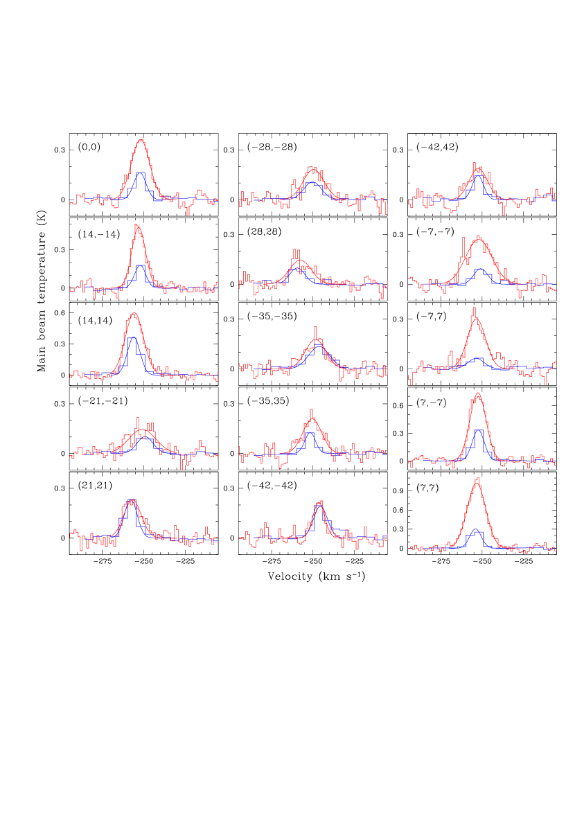
Figure 2: Same as Fig. 1, but for selected positions in the BCLMP302 region.

In this subsection we consider a source with narrow [C ii], [C i] and CO emission lines observed in the Milky Way — the dark cloud L1599B which is a portion of the molecular ring at $\simeq 27$ pc from the star $\Lambda$ Ori located at a distance of 425 pc (Goldsmith et al. 2016). Observations of the [C ii] FS line were obtained with the SOFIA (Stratospheric Observatory for Infrared Astronomy) airborne observatory, while the [C i] $J=1$–0, ¹²CO and ¹³CO $J=1$–0 and 2–1, and ¹²CO $J=3$–2 data were collected with the Purple Mountain Observatory and APEX (Atacama Pathfinder EXperiment) telescopes. The line profiles shown in Fig. 2 of Goldsmith et al. (2016) allow us to select symmetric lines observed towards two positions O3 and O1 within the L1599B cloud. Their local standard of rest (LSR) radial velocities are listed in Table 2. The ¹³CO(2-1) line towards O1 was not detected.

Table 2 also includes the [C i] ³P₁–³P₀ transition at $\omega=492160.651(55)$ MHz (Yamamoto & Saito 1991). The corresponding uncertainty $\sigma_{v}$([C i]) = 0.034 km s^-1 is almost six times lower than that of [C ii] and, thus, the combination of [C ii] + [C i] imposes the same systematic error on $\Delta\alpha/\alpha$ as does the [C ii] line alone, i.e. $\sigma_{\rm sys}=3\times 10^{-7}$. In Table 2, the rest frame frequency of the ¹²CO $J=3-2$ transition is $\omega=345795.9899(5)$ MHz, and $\omega=220398.70056(12)$ MHz for the strongest among the hyper-fine structure (HFS) lines of ¹³CO $J=2-1$, $F=5/2-3/2$ (Endres et al. 2016). We note that the three HFS lines of the ¹³CO $J=2-1$ transition are split by 0.11 km s^-1 between the strongest and the weakest ($F=3/2-3/2$) lines which bracket this interval. The intensity of the weakest line is about 10 times lower as compared with the strongest component, whereas the middle line with $F=3/2-1/2$ and half the intensity of the strongest component is split from the latter by only 0.045 km s^-1. These HFS lines are not resolved in observations of the O3 and O1 regions since their widths (FWHM) are larger than 0.5 km s^-1.

According to Goldsmith et al. (2016), the listed emission lines were observed with the following angular resolutions (FWHM): $\theta$([C ii]) = $15^{\prime\prime}$, $\theta$([C i]) = $12.4^{\prime\prime}$, $\theta$(¹²CO_3-2) = $17.5^{\prime\prime}$, and $\theta$(¹²CO_2-1) = $\theta$(¹³CO_2-1) = $27^{\prime\prime}$–$28^{\prime\prime}$. The ¹²CO(1-0) line was not included in Table 2 since it was observed with a beam size $\theta=50^{\prime\prime}$ albeit its radial velocity is consistent with the other data.

At first, for each dataset O3 and O1, we average the radial velocities of CO transitions and compare their mean weighted values with $V_{\rm[C\,II]}$. The results obtained by averaging with weights inversely proportional to $\sigma^{2}_{\scriptscriptstyle{\Delta V}}$ are $\langle V_{\rm CO}\rangle=8.75\pm 0.04$ km s^-1 (O3), and $\langle V_{\rm CO}\rangle=11.40\pm 0.01$ km s^-1 (O1). This leads to the following constraints on variations in $\alpha$: $\Delta\alpha/\alpha=(1\pm 2_{\rm stat}\pm 3_{\rm sys})\times 10^{-7}$ (O3), and $\Delta\alpha/\alpha=(7\pm 2_{\rm stat}\pm 3_{\rm sys})\times 10^{-7}$ (O1).

Then, we calculate the mean radial velocities for the combination [C ii] + [C i]: $\langle V_{\rm[C\,II]+[C\,I]}\rangle=8.889\pm 0.016$ km s^-1 (O3), and $\langle V_{\rm[C\,II]+[C\,I]}\rangle=11.25\pm 0.07$ km s^-1 (O1). This combination gives slightly lower random errors: $\Delta\alpha/\alpha=(-2.3\pm 0.7_{\rm stat}\pm 3.0_{\rm sys})\times 10^{-7}$ (O3), and $\Delta\alpha/\alpha=(2.5\pm 1.2_{\rm stat}\pm 3.0_{\rm sys})\times 10^{-7}$ (O1). Both results are consistent with zero fractional changes in $\alpha$ at the level restricted by the laboratory error of the [C ii] FS transition.

The same order of magnitude bound on $\alpha$ variation can be obtained from the analysis of the five Galactic molecular clouds where the mean velocity offset $\langle\Delta V\rangle=0.022\pm 0.082_{\rm stat}\pm 0.034_{\rm sys}$ km s^-1 between the [C i] $J=1-0$ and ¹³CO $J=1-0$, $J=2-1$ transitions was found in Levshakov, Molaro & Reimers (2010). When interpreted in terms of $\alpha$ variation, it gives $\Delta\alpha/\alpha=(0.4\pm 1.4_{\rm stat}\pm 0.6_{\rm sys})\times 10^{-7}$. The advantage of the combination of the [C i] and CO transitions is in a lower systematic error. Thus, $\Delta\alpha/\alpha$ is restricted to a few $10^{-7}$ in the Milky Way and, as we will see below, also in the nearby galaxy M33.

Table 2: Radial velocities $V_{\scriptscriptstyle\rm LSR}$ (in km s^-1) and their $1\sigma$ errors measured at the selected positions O3 and O1 towards L1599B (Goldsmith et al. 2016).

Spectral Line	O3		O1		Beam size
					(FWHM),
					arcsec
[C ii] 2P3/2–2P1/2	8.70$\pm$	0.12	11.0$\pm$	0.1	15
12CO $J$=2–1	8.93$\pm$	0.03	11.39$\pm$	0.01	27-28
12CO $J$=3–2	8.73$\pm$	0.01	11.41$\pm$	0.01	17.5
13CO $J$=2–1	8.76$\pm$	0.02	$-$		27-28
[C i] 3P1–3P0	8.89$\pm$	0.01	11.27$\pm$	0.03	12.4

2.2 The galaxy M33

For the recent years, the Herschel observatory explored a large number of nearby galaxies in the FS [C ii] 158 $\mu$m line. In this section, we use results of the precise measurements of [C ii] emission in the nearby Triangulum galaxy M33 located at a distance of about $D\sim 800$ kpc (McConnachie et al. 2009; Brunthaler et al. 2005), namely, three H ii regions located either near the centre of M33 or a few kpc to the north.

The CO(2-1) emission towards the disk of M33 was mapped at the 30m IRAM (Institute for Radio Astronomy in the Millimeter Range) telescope with a resolution $12^{\prime\prime}\times 2.6$ km s^-1 (Gratier et al. 2010). The H ii regions BCLMP691 and BCLMP302 (3.3 kpc and 2 kpc to the north of the dynamical centre of M33, respectively) and the centre of M33 itself were mapped in the [C ii] line with the HIFI (Heterodyne Instrument for the Far Infrared) spectrometer onboard the Herschel satellite with the same $12^{\prime\prime}$ angular resolution and 1.2 km s^-1 spectral resolution after smoothing (Mookerjea et al. 2016; Braine et al. 2012).

Table 3 gives the positions of the spectra (first two columns) with respect to the (0,0) offsets which are (J2000) RA = 01:34:16.40, Dec = 30:51:54.6 for the BCLMP691 region (Braine et al. 2012), RA = 01:33:48.20, Dec = 30:39:21.4 for the central region, and RA = 01:34:06.30, Dec = 30:47:25.3 for the BCLMP302 region, respectively (Mookerjea et al. 2016). Columns 3 and 4 give the LSR radial velocities and their uncertainties indicated in parentheses which are results of one-component Gaussian fits provided by the CLASS fitting routine. The data for the BCLMP691 region are taken from Table 1 in Braine et al. (2012), whereas the line positions and their errors for the central region and BCLMP302 are calculated in the present paper and the one-component Gaussian fits are shown in Figs. 1 and 2. The velocity offsets $\Delta V=V_{\rm rot}-V_{\rm fs}$ are given in the last column 5.

In total, Table 3 lists 46 positions where velocity offsets are known with different uncertainties, $\sigma_{\scriptscriptstyle{\Delta V}}$. Being averaged with weights inversely proportional to $\sigma^{2}_{\scriptscriptstyle{\Delta V}}$, the mean offset is equal to $\langle\Delta V\rangle=-0.01\pm 0.14$ km s^-1. Using Eq.(4), one gets $\Delta\alpha/\alpha=(-0.1\pm 2.4_{\rm stat}\pm 3.0_{\rm sys})\times 10^{-7}$. The result obtained shows no changes in $\alpha$ at the sensitivity level which is determined by the currently available precision of the laboratory frequencies.

Table 3: Selected positions observed in [C ii] and CO(2-1) emission towards M33. Given in parentheses are statistical errors $(1\sigma)$.

$x(^{\prime\prime})$		$y(^{\prime\prime})$		$V_{\rm[C\,II]}$	$V_{\rm CO}$	$\Delta V$
				km s-1	km s-1	km s-1
BCLMP691
$-1$.	9	$-4$.	6	$-269.6(0.2)$	$-269.5(0.2)$	0.1(0.3)
6.	5	2.	7	$-268.9(0.2)$	$-268.9(0.2)$	0.0(0.3)
4.	6	$-1$.	9	$-269.0(0.3)$	$-269.0(0.2)$	0.0(0.4)
$-2$.	7	6.	5	$-268.8(0.2)$	$-268.6(0.2)$	0.2(0.3)
$-3$.	8	$-9$.	2	$-268.9(0.6)$	$-269.0(0.3)$	$-0.1(0.7)$
3.	8	9.	2	$-269.2(0.7)$	$-269.1(0.5)$	0.1(0.9)
$-6$.	5	$-2$.	7	$-269.3(0.2)$	$-269.3(0.4)$	0.0(0.4)
$9$.	2	$-3$.	8	$-265.1(0.4)$	$-266.9(0.1)$	$-1.8(0.4)$
$-9$.	2	3.	8	$-268.3(0.5)$	$-268.2(0.7)$	0.1(0.9)
2.	7	$-6$.	5	$-269.4(0.2)$	$-269.4(0.2)$	0.0(0.3)
1.	9	4.	6	$-269.1(0.2)$	$-269.3(0.2)$	$-0.2(0.3)$
13.	9	$-5$.	7	$-265.1(0.4)$	$-266.1(0.2)$	$-1.0(0.4)$
$-4$.	6	1.	9	$-269.1(0.2)$	$-269.4(0.2)$	$-0.3(0.3)$
9.	6	23.	1	$-267.5(0.7)$	$-267.2(0.4)$	0.3(0.8)
18.	5	$-7$.	7	$-266.7(0.7)$	$-265.9(0.4)$	0.8(0.8)
0.	0	0.	0	$-269.4(0.1)$	$-269.9(0.2)$	$-0.5(0.2)$
M33 centre
0.	0	0.	0	$-165.8(0.2)$	$-165.1(0.3)$	0.7(0.4)
$-12$.	0	$-28$.	0	$-157.2(0.6)$	$-158.8(0.3)$	$-1.6(0.7)$
$12$.	0	$28$.	0	$-185.8(0.2)$	$-182.9(0.8)$	$2.9(0.8)$
$-15$.	0	$-37$.	0	$-155.0(0.3)$	$-156.0(0.2)$	$-1.0(0.4)$
$15$.	0	$37$.	0	$-189.6(0.2)$	$-190.5(0.1)$	$-0.9(0.2)$
$-19$.	0	$-46$.	0	$-154.4(0.2)$	$-153.5(0.3)$	$0.9(0.4)$
$19$.	0	$46$.	0	$-195.6(0.4)$	$-193.4(0.2)$	$2.2(0.4)$
$-23$.	0	$-55$.	0	$-150.9(0.5)$	$-149.9(0.3)$	$1.0(0.6)$
$23$.	0	$55$.	0	$-195.2(0.7)$	$-196.6(0.2)$	$-1.4(0.7)$
$44$.	0	$12$.	0	$-169.4(0.5)$	$-171.0(0.9)$	$-1.6(1.0)$
$-4$.	0	$-9$.	0	$-164.0(0.6)$	$-162.8(0.5)$	1.2(0.8)
$4$.	0	$9$.	0	$-170.9(0.2)$	$-168.5(0.1)$	2.4(0.2)
$53$.	0	$8$.	0	$-170.6(0.3)$	$-170.5(0.2)$	0.1(0.4)
62.	0	4.	0	$-170.6(0.2)$	$-170.1(0.3)$	0.5(0.4)
72.	0	0.	0	$-169.7(0.5)$	$-167.0(0.7)$	2.7(0.9)
BCLMP302
0.	0	0.	0	$-252.0(0.2)$	$-252.3(0.4)$	$-0.3(0.4)$
14.	0	$-14$.	0	$-253.1(0.2)$	$-252.2(0.4)$	0.9(0.4)
14.	0	14.	0	$-255.7(0.2)$	$-256.1(0.1)$	$-0.4(0.2)$
$-21$.	0	$-21$.	0	$-250.9(0.7)$	$-249.2(0.5)$	1.7(0.9)
$21$.	0	$21$.	0	$-256.8(0.3)$	$-257.9(0.3)$	$-1.1(0.4)$
$-28$.	0	$-28$.	0	$-249.6(0.7)$	$-250.2(0.4)$	$-0.6(0.8)$
$28$.	0	$28$.	0	$-257.7(0.6)$	$-259.5(0.5)$	$-1.8(0.8)$
$-35$.	0	$-35$.	0	$-248.5(0.5)$	$-246.3(0.4)$	$2.2(0.6)$
$-35$.	0	$35$.	0	$-250.5(0.5)$	$-251.7(0.5)$	$-1.2(0.7)$
$-42$.	0	$-42$.	0	$-246.5(0.4)$	$-245.5(0.2)$	$1.0(0.4)$
$-42$.	0	$42$.	0	$-252.3(0.6)$	$-252.6(0.2)$	$-0.3(0.6)$
$-7$.	0	$-7$.	0	$-252.1(0.5)$	$-250.9(0.7)$	$1.2(0.9)$
$-7$.	0	7.	0	$-253.5(0.3)$	$-253.7(0.7)$	$-0.2(0.8)$
7.	0	$-7$.	0	$-252.6(0.2)$	$-252.4(0.2)$	0.2(0.3)
7.	0	7.	0	$-253.5(0.1)$	$-254.1(0.1)$	$-0.6(0.1)$

2.3 High-redshift [C ii]/CO systems

Here we take up a sample of five $z>5.7$ quasars with detected [C ii] FS and CO rotational transitions. As mentioned in Sect. 1, the electron-to-proton mass ratio is stable to an accuracy of a few $10^{-6}$ up to redshift $z\sim 4$. In this case, the FST method can be applied for estimating changes in $\alpha$ within the interval $10^{-5}\;\raise 1.29167pt\hbox{$<$\kern-7.5pt\raise-4.73611pt\hbox{$\sim$}}\;|\Delta\alpha/\alpha|\;\raise 1.29167pt\hbox{$<$\kern-7.5pt\raise-4.73611pt\hbox{$\sim$}}\;10^{-4}$.

At present, the accuracy of the high-$z$ estimates of $\Delta\alpha/\alpha$ by the FST method is about two orders of magnitude lower as compared with the local Universe because high-redshift objects are fainter, signal-to-noise ratios are lower, and spectral resolution is moderate. Nevertheless, this method has a perspective since it enables us to test $\alpha$ at cosmological epochs which are not accessible to optical spectroscopy.

The selected sources showing symmetric emission line profiles are listed in Table 4. Column 1 provides the quasar names, columns 2 and 3 give the measured redshifts of the [C ii] 158 $\mu$m and CO lines as described below, and the velocity offsets $\Delta V=V_{\rm CO}-V_{\rm[C\,II]}=c(z_{\rm CO}-z_{\rm[C\,II]})/(1+\bar{z})$ are presented in column 4 (here $\bar{z}$ is the mean redshift).

J0129–0035. The [C ii] line was observed at $z=5.8$ with the Atacama Large Millimeter/submillimeter Array (ALMA) at $0.57^{\prime\prime}\times 0.49^{\prime\prime}$ resolution (Fig. 5 in Wang et al. 2013), while the CO(6-5) line was observed at 3 mm with the IRAM Plateau de Bure Interferometer (PdBI) at $\sim 5^{\prime\prime}$ resolution (Fig. 2 in Wang et al. 2011). Table 4 gives the host galaxy redshifts measured with the [C ii] and CO(6-5) lines.

J2310+1855. Both the [C ii] and CO(6-5) lines were detected at $z=6.0$ by Wang et al. (2013). [C ii] was observed with ALMA at $0.72^{\prime\prime}\times 0.51^{\prime\prime}$ resolution, while the CO(6-5) line was observed with the PdBI at the beam size $5.4^{\prime\prime}\times 3.9^{\prime\prime}$ (Figs. 1 and 5 in Wang et al. 2013). The measured redshifts of these lines are listed in Table 4.

J2054–0005. The [C II] emission line was observed at $z=6.0$ with ALMA at $0.64^{\prime\prime}\times 0.58^{\prime\prime}$ resolution (Fig. 5 in Wang et al. 2013), while CO(6-5) was detected with the PdBI at $\sim 5^{\prime\prime}$ resolution (Fig. 1 in Wang et al. 2010). The redshifts of these lines are given in Table 4.

J1319+0950. The [C ii] emission line was observed at $z=6.1$ with a synthesized beam size of $0.69^{\prime\prime}\times 0.49^{\prime\prime}$ using ALMA (Fig. 5 in Wang et al. 2013). Wang et al. (2011) show in their Fig. 1 the observed profile of the CO(6-5) line which was obtained with the 3 mm receiver on the PdBI at $\sim 3.5^{\prime\prime}$ resolution The measured redshifts are presented in Table 4.

J1148+5251. The CO(7-6) and (6-5) emission lines were detected at $z=6.4$ by Bertoldi et al. (2003) using the PdBI at $\sim 5^{\prime\prime}$ resolution. The observed spectra of CO(7-6) and (6-5) are shown in their Fig. 1. The measured redshifts of $z_{\rm CO(7-6)}=6.4192\pm 0.0009$ and $z_{\rm CO(6-5)}=6.4187\pm 0.0006$ yield the mean value $\langle z_{\rm CO}\rangle=6.4190\pm 0.0005$ which is listed in Table 4. The [C ii] line emission redshifted to $z=6.4189\pm 0.0006$ was observed by Maiolino et al. (2005) with the IRAM 30m telescope at $9.6^{\prime\prime}$ resolution (see their Fig. 1). On the other hand, Walter et al. (2009) who used the PdBI at $\sim 0.3^{\prime\prime}$ resolution determined a central velocity of the [C ii] line of $3\pm 12$ km s^-1 relative to the CO redshift of $z=6.419$ (see their Fig. 2), which leads to $z_{\rm[C\,II]}=6.4189\pm 0.0003$. Both results yield the mean $\langle z_{\rm[C\,II]}\rangle=6.4189\pm 0.0003$ given in Table 4.

These five velocity offsets $\Delta V$, being averaged with weights inversely proportional to their uncertainties squared, yield $\langle\Delta V\rangle=0\pm 8$ km s^-1, and thus $|\Delta\alpha/\alpha|<1.3\times 10^{-5}$ at redshift $z=5.7-6.5$. The result obtained improves by five times our previous constraint on $\Delta\alpha/\alpha$ at $z=6.4$ (Levshakov et al. 2008). Thus, we may conclude that $\alpha$ does not vary at the level of $\sim 10^{-5}$ up to $z=6.5$, corresponding to 5% of the age of the Universe today.

To complete this section we note that the [C ii] 158 $\mu$m emission was observed towards a number of distant quasars and galaxies with $z>6$ where the CO lines have not yet been detected. These objects are listed in Table 5. The redshifts for some of them were also determined from the Mg ii $\lambda 2798$ Å low ionization line, and it is tempting to use the measured redshifts $z_{\rm Mg\,II}$ and $z_{\rm[C\,II]}$ to put constraints on $\Delta\alpha/\alpha$, for the ratio of frequencies of the FS to the optical gross-structure transitions is proportional to $\alpha$ squared (FST method, see Sect. 1). However, for the $z>6$ objects, it was found that the peaks of the Mg ii and [C ii] or CO lines show significant offsets from each other with the Mg ii line being blueshifted by $\Delta V=-480\pm 630$ km s^-1 (Venemans et al. 2016), which inhibits accurate measurements of $\Delta\alpha/\alpha$ using optical spectra. We can only hope that other molecular lines which closely trace the [C ii] 158 $\mu$m emission will be detected in the future. Then more stringent limits than our $10^{-5}$ value on $\Delta\alpha/\alpha$ could be obtained by radio methods for this early cosmological epoch.

Table 4: Velocity offsets $\Delta V=c(z_{\rm CO}-z_{\rm[C\,II]})/(1+\bar{z})$ for the $z>5.7$ quasars. Given in parentheses are statistical errors $(1\sigma)$. References: (1) Wang et al. 2013, (2) Wang et al. 2011, (3) Wang et al. 2010, (4) Bertoldi et al. 2003, (5) Maiolino et al. 2005, (6) Walter et al. 2009.

Name	$z_{\rm[C\,II]}$	$z_{\rm CO}$	$\Delta V$, km s-1
J0129–0035	5.7787(1)1	5.7794(8)2	31$\pm$	35
J2310+1855	6.0031(2)1	6.0025(7)1	$-30$$\pm$	30
J2054–0005	6.0391(1)1	6.0379(22)3	$-50$$\pm$	90
J1319+0950	6.1330(7)1	6.1321(12)2	$-40$$\pm$	60
J1148+5251	6.4189(3)5,6	6.4190(5)4	4$\pm$	12

Table 5: [C ii] measurements for the $z>6$ quasars and galaxies without detected CO lines. Given in parentheses are statistical errors $(1\sigma)$. References: (1) Willott et al. 2015a, (2) Willott et al. 2015b, (3) Jones et al. 2017, (4) Willott et al. 2013, (5) Venemans et al. 2016, (6) Brada$\check{c}$ et al. 2017, (7) Smit et al. 2017, (8) Venemans et al. (2017).

Name	$z_{\rm[C\,II]}$	Name	$z_{\rm[C\,II]}$
J0055+0146	6.0060(8)1	RXJ1347:1216	6.7655(5)6
WMH 5	6.0695(3)2,3	J0109–3047	6.7909(4)5
J2229+1457	6.1517(5)1	COS2987030247	6.8076(2)7
CLM 1	6.1657(3)2	COS3018555981	6.8540(3)7
J0210–0456	6.4323(5)4	J2348–3054	6.9018(7)5
J0305–3150	6.6145(1)5	J1120+0641	7.0851(5)8

3 Summary and Conclusions

In this work, we present an analysis of [C i], [C ii], and CO lines of one molecular cloud in the disk of the Milky Way, three H ii zones in the neighbour galaxy M33, and five quasar systems at $z=5.7-6.5$.

To obtain a limit on $\Delta\alpha/\alpha$ by the Fine Structure Transition (FST) method (Levshakov & Kozlov 2017), we used recently published observations with the Herschel and SOFIA observatories, the Purple Mountain Observatory, APEX, ALMA, and IRAM telescopes.

At low redshifts, the FST method produces results which agree quantitatively with those obtained by other methods. However, at high redshifts, it has the distinct advantage over optical spectral observations which are applicable to cosmological tests of $\Delta\alpha/\alpha$ only up to $z\;\raise 1.29167pt\hbox{$<$\kern-7.5pt\raise-4.73611pt\hbox{$\sim$}}\;4$. The comparison between optical and radio constraints on $\Delta\alpha/\alpha$ based on the most accurate recent observations is shown in Fig. 3.

Our main conclusions are as follows:

• Using a combination of the [C ii] and [C i] fine structure (FS) lines, ¹²CO(2-1), (3-2), and ¹³CO(2-1) being observed towards two positions of the dark molecular cloud L1599B in our Galaxy, we set a limit on $|\Delta\alpha/\alpha|<3\times 10^{-7}$. This limit is in agreement with $|\Delta\alpha/\alpha|<2\times 10^{-7}$ resulting from the analysis of five Galactic molecular clouds using [C i] FS, and ¹³CO(2-1), (1-0) lines (Levshakov, Molaro & Reimers 2010).

• From the relative positions of the [C ii] FS and CO(2-1) emission lines observed towards three H ii regions of M33, we find the most stringent constraint to date on $\alpha$ variation of $|\Delta\alpha/\alpha|<4\times 10^{-7}$ for the neighbour galaxy.

• The most distant quasar systems from the redshift range $z=5.7-6.5$ with detected [C ii] FS and CO(6-5), (7-6) emission show no changes in $\alpha$ at the level of $|\Delta\alpha/\alpha|<1.3\times 10^{-5}$.

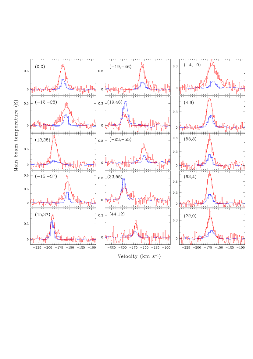
Figure 1: Shown by histograms are the [C ii] (red) and CO(2-1) (blue) spectra at selected positions in the centre of M33. The one-component Gaussians of the corresponding colours are the fits to the observed spectra. The selected positions in arcsec are indicated in parentheses. The same positions are listed in Table 3.

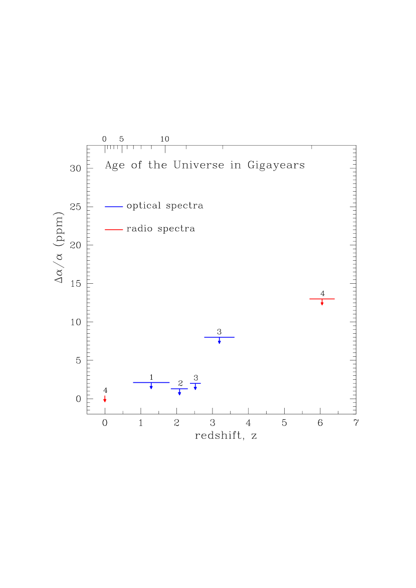
Figure 3: The observational constraints on $\Delta\alpha/\alpha$ in parts per million (ppm) from optical (blue) and radio (red) observations plotted versus redshift, $z$. The age of the Universe in Gigayears is shown on the top axis. The horizontal bars indicate the covered redshift ranges where the $1\sigma$ upper bounds were calculated. The redshift range of the low redshift radio constraints (Milky Way and M33) is unresolved at the scale of this plot. The plot illustrates that all available optical constraints are restricted by $z\;\raise 1.29167pt\hbox{$<$\kern-7.5pt\raise-4.73611pt\hbox{$\sim$}}\;4$. References: 1 – Evans et al. 2014; 2 – Murphy et al. 2017; 3 – King et al. 2012; 4 – this paper.

References

- (1) Agafonova I. I., Molaro P., Levshakov S. A., Hou J. L., 2011, A&A, 529, 28
- (2) Bagdonaite J., Ubachs W., Murphy M. T., Whitmore J. B. 2015, PRL, 114, 071301
- (3) Bagdonaite J., Jansen P., Henkel C., Bethlem H. L., Menten K. M., Ubachs W., 2013a, Sci., 339, 46
- (4) Bagdonaite J., Daprà M., Jansen P., Bethlem H. L., Ubachs W., Muller S., Henkel C., Menten K. M., 2013b, PRL, 111, 231101
- (5) Bainbridge M. B., Barstow M. A., Reindl N., Tchang-Brillet W.-Ü., Ayres T., Webb J., Barrow J., Hu J., et al., 2017, Univese, 3, 32
- (6) Bertoldi F., Cox P., Neri R., Carilli C. L., Walter F., Omont A., Beelen A., Henkel C., et al., 2003, A&A, 409, L47
- (7) Brada M., Garcia-Appadoo D., Huang K.-H., Vallini L., Finney E. Q., Hoag A., Lemaux B. C., Schmidt K. B., et al., 2017, ApJ, 836, L2
- (8) Braine J., Gratier P., Kramer C., Israel F. P., van der Tak F., Mookerjea B., Boquien M., Tabatabaei F., et al., 2012, A&A, 544, A55
- (9) Brax P., 2014, PhRvD, 90, 023505
- (10) Brunthaler A., Reid M. J., Falcke H., Greenhill L. J., Henkel C., 2005, Sci., 307, 1440
- (11) Cooksy A. L., Blake G. A., Saykally R. J., 1986a, ApJL, 305, L89
- (12) Curran S. J., Tanna A., Koch F. E., Berengut J. C., Webb J. K., Stark A. A., Flambaum V. V., 2011, A&A, 533, A55
- (13) Daprà M., Henkel C., Levshakov S. A., Menten K. M., Muller S., Bethlem H. L., Leurini S., Lapinov A. V., Ubachs W., 2017a, MNRAS (submit.)
- (14) Daprà M., van der Laan M., Murphy M. T., Ubachs W. 2017b, MNRAS, 465, 4057
- (15) Daprà M., Noterdaeme P., Vonk M., Murphy M. T., Ubachs W., 2017c, MNRAS, 467, 3848
- (16) Davis E. D., Hamdan L., 2015, PhRvC, 92, 014319
- (17) de Blok W. J. G., Walter F., Smith J.-D. T., et al., 2016, AJ, 152, 51
- (18) Ellingsen S. P., Voronkov M. A., Breen S. L., Lovell J. E. J., 2012, ApJ, 747, L7
- (19) Endres C. P., Schlemmer S., Schilke P., Stutzki J., Müller H. S. P., 2016, J. Mol. Spectrosc., 327, 95
- (20) Evans T. M., Murphy M. T., Whitmore J. B., Misawa T., Centurión M., D’Odorico S., Lopez S., Martins C. J. A. P., et al., 2014, MNRAS, 445, 128
- (21) Flambaum V. V. 2007, Int. J. Mod. Phys. A, 22, 4937
- (22) Gao H., Wu X. F., Mészáros P., 2015, ApJ, 810, 121
- (23) Godun R. M., Nisbet-Jones P. B. R., Jones J. M., King S. A., Johnson L. A. M., Margolis H. S., Szymaniec K., Lea S. N., et al., 2014, PhRvL, 113, 210801
- (24) Goldsmith P. F., Pineda J. L., Langer W. D., Liu T., Requena-Torres M., Ricken O., Riquelme D., 2016, ApJ, 824, 141
- (25) Gratier P., Braine J., Rodriguez-Fernandez N. J., Schuster K. F., Kramer C., Xilouris E. M., Tabatabaei F. S., Henkel C., et al. 2010, A&A, 522, A3
- (26) Hemmati S., Yan L., Diaz-Santos T., Armus L., Capak P., Faisst A., Masters D., 2017, ApJ, 834, 36
- (27) Henkel C., Menten K. M., Murphy M. T., Jethava N., Flambaum V. V., Braatz J. A., Muller S., Ott J., Mao R. O., 2009, A&A, 500, 725
- (28) Hojjati A., Plahn, A., Zucca A., Pogosian L., Brax P., Davis A.-C., Zhao G.-B., 2016, PhRvD, 93, 043531
- (29) Huntemann N., Sanner C., Lipphardt B., Tamm C., Peik E., 2016, PhRvL, 116, 063001
- (30) Jones G. C., Willott C. J., Carilli C. L., A. Ferrara A., Wang R., Wagg J., 2017, eprint arXiv: 1706.09968
- (31) Kanekar N., 2011, ApJ, 728, L12
- (32) Kanekar N., Ubachs W., Menten K. M., Bagdonaite J., Brunthaler A., Henkel C., Muller S., Bethlem H. L., Daprà M., 2015, MNRAS, 448, L104
- (33) King, J. A., Webb, J. K., Murphy, M. T., Flambaum, V. V., Carswell, R. F., Bainbridge, M. B., Wilczynska, M. R., Koch, F. E., 2012, MNRAS, 422, 3370
- (34) King J. A., Murphy M. T., Ubachs W., Webb, J. K., 2011, MNRAS, 417, 3010
- (35) King J. A., Webb J. K., Murphy M. T., Carswell R. F., 2008, PRL, 101, 251304
- (36) Kostelecký V. A., Lehnert R., Perry M. J., 2003, PhRvD, 68, 123511
- (37) Kotu S. M., Murphy M. T., Carswell R. F., 2017, MNRAS, 464, 3679
- (38) Kozlov M. G., Levshakov S. A., 2013, Ann. Phys., 525, 452
- (39) Kozlov M. G., Porsev S. G., Levshakov S. A., Reimers D., Molaro P., 2008, PhRvA, 77, 032119
- (40) Langacker P., Segrè G., Strassler J., 2002, Phys. Lett. B, 528, 121
- (41) Leefer N., Weber C. T. M., Cingöz A., Torgerson J. R., Budker D., 2013, PhyRvL, 111, 060801
- (42) Levshakov S. A., 2016, in Proceed. of the conf. Radiation mechanisms of astrophysical objects: classics today, eprint arXiv: 1603.01262
- (43) Levshakov S. A., Kozlov M. G. 2017, MNRAS, 469, L16
- (44) Levshakov S. A., Reimers D., Henkel C., Winkel B., Mignano A., Centurión M., Molaro P., 2013, A&A, 559, A91
- (45) Levshakov S. A., Combes F., Boone F., Agafonova I. I., Reimers D., Kozlov M. G., 2012, A&A, 540, L9
- (46) Levshakov S. A., Kozlov M. G., Reimers D., 2011, ApJ, 738, 26
- (47) Levshakov S. A., Molaro P., Reimers D., 2010, A&A, 516, A113
- (48) Levshakov S. A., Reimers D., Kozlov M. G., Porsev S. G., Molaro P., 2008, A&A, 479, 719
- (49) Levshakov S. A., Centurión M., Molaro P., D’Odorico S., Reimers D., Quast R., Pollmann M., 2006, A&A, 449, 879
- (50) Liberati S., 2013, Class. Quant. Grav., 30, 133001
- (51) Maiolino R., Cox P., Caselli P., Beelen A., Bertoldi F., Carilli C. L., Kaufman M. J., Menten K. M., et al., 2005, A&A, 440, L51
- (52) Marshall M. A., Ellingsen S. P., Lovell J. E. J., Dickey J. M., Voronkov M. A., Breen S. L., 2017, MNRAS, 466, 2450
- (53) Martins C. J. A. P., Pinho A. M. M., 2017, PhRvD, 95, 023008
- (54) McConnachie A. W., Irwin M. J., Ibata R. A., Dubinski J., Widrow L. M., Nicolas F., Cté P., Dotter A. L., et al., 2009, Nat., 461, 66
- (55) Molaro P., Centurión M., Whitmore J. B., Evans T. M., Murphy M. T., Agafonova I. I., Bonifacio P., D’Odorico S., et al., 2013, A&A, 555, A68
- (56) Mookerjea B., Israel F., Kramer C., Nikola T., Braine J., Ossenkopf V., Röllig M., Henkel C., et al., 2016, A&A, 586, A37
- (57) Murphy M. T., Malec A. L., Prochaska J. X., 2017, MNRAS, 464, 2609
- (58) Nicholson T. L., Campbell S. L., Hutson R. B., Marti G. E., Bloom B. J., McNally R. L., Zhang W., Barrett M. D., et al., 2015, Nat. Comm., 6, 6896
- (59) Nisbet-Jones P. B. R., King S. A., Jones J. M., Godun R. M., Baynham C. F. A., Bongs K., Doleal M., Balling P., Gill P., 2016, Applied Phys. B, 122, 57
- (60) Nunes R. C., Bonilla A., Pan S., Saridakis E. N. 2017, Eur. Phys. J. C, 77, 230
- (61) Petitjean P., Wang F. Y., Wu X. F., Wei J. J., 2016, SpScRv, 202, 195
- (62) Quast R., Reimers D., Levshakov S. A., 2004, A&A, 415, L7
- (63) Rahmani H., Wendt M., Srianand R., Noterdaeme P., Petitjean P., Molaro P., Whitmore J. B., Murphy M. T., et al. 2013, MNRAS, 435, 861
- (64) Rosenband T., Hume D. B., Schmidt P. O., Chou C. W., Brusch A., Lorini L., Oskay W. H., Drullinger R. E., et al., 2008, Science, 319, 1808
- (65) Smit, R., Bouwens, R. J., Carniani, S., Oesch, P. A., Labbé, I., Illingworth, G. D., van der Werf, P., Bradley, L. D., et al. 2017, eprint arXiv: 1706.0461
- (66) Thompson R., 2017, MNRAS, 467, 4558
- (67) Uzan J.-P., 2011, Living Rev. Relativity 14, 2
- (68) Vasquez F. A., Rahamani H., Noterdaeme N., Petitjean P., Srianand R. Ledoux, C., 2014, A&A, 562, A88
- (69) Venemans B. P., Walter F., Decarli R., Baados E., Hodge J., Hewett P., McMahon R. G., Mortlock D. J., Simpson C., 2017, ApJ, 837, 146
- (70) Venemans B. P., Walter F., Zschaechner L., Decarli R., De Rosa G., Findlay J. R., McMahon R. G., Sutherland W. J., 2016, ApJ, 816, 37
- (71) Walter F., Riechers D., Cox P., Neri R., Carilli C., Bertoldi F., Weiss A., Maiolono R., 2009, Nature, 457, 699
- (72) Wang R., Wagg J., Carilli C. L., Walter F., Lentati L., Fan X., Riechers D. A., Bertoldi F., et al., 2013, ApJ, 773, 44
- (73) Wang R., Wagg J., Carilli C. L., Neri R., Walter F., Omont A., Riechers D. A., Bertoldi F., et al., 2011, AJ, 142, 101
- (74) Wang R., Carilli C. L., Neri R., Riechers D. A., Wagg J., Walter F., Bertoldi F., Menten K. M., et al., 2010, ApJ, 714, 699
- (75) Wei J. J., Wang J. S., Gao H., Wu X. F., 2016, ApJ, 818, L2
- (76) Wendt M., Molaro P., 2012, A&A, 541, A69
- (77) Wendt M., Reimers D., 2008, EPJ Special Topics, 163, 197206
- (78) Weiß A., Walter F., Downes D., Carrili C. L., Henkel C., Menten K. M., Cox P., 2012, ApJ, 753, 102
- (79) Willott C. J., Bergeron J., Omont A., 2015a, ApJ, 801, 123
- (80) Willott C. J., Carilli C. L., Wagg J., Wang R. 2015b, ApJ, 807, 180
- (81) Willott C. J., Omont A., Bergeron J., 2013, ApJ, 770, 13
- (82) Yamamoto S., Saito, S., 1991, ApJ, 370, L103