Elastic three-sphere microswimmer in a viscous fluid

Abstract

We discuss the dynamics of a generalized three-sphere microswimmer in which the spheres are connected by two elastic springs. The natural length of each spring is assumed to undergo a prescribed cyclic change. We analytically obtain the average swimming velocity as a function of the frequency of the cyclic change in the natural length. In the low-frequency region, the swimming velocity increases with the frequency and its expression reduces to that of the original three-sphere model by Najafi and Golestanian. In the high-frequency region, conversely, the average velocity decreases with increasing the frequency. Such a behavior originates from the intrinsic spring relaxation dynamics of an elastic swimmer moving in a viscous fluid.

Microswimmers are tiny machines that swim in a fluid such as sperm cells or motile bacteria, and are expected to be applied to microfluidics and microsystems Lauga092 . By transforming chemical energy into mechanical work, microswimmers change their shape and move in viscous environments. Over the length scale of microswimmers, the fluid forces acting on them are governed by the effect of viscous dissipation. According to Purcell’s scallop theorem Purcell77 , time-reversal body motion cannot be used for locomotion in a Newtonian fluid Lauga11 . As one of the simplest models exhibiting broken time-reversal motion, Najafi and Golestanian proposed a three-sphere swimmer Golestanian04 ; Golestanian08 , where three in-line spheres are linked by two arms of varying length. This model is suitable for analytical analysis because it is sufficient to consider only the translational motion and the tensorial structure of the fluid motion can be neglected. Recently, such a swimmer has been experimentally realized by using ferromagnetic particles at an air-water interface and applying an oscillating magnetic field Grosjean .

The original Najafi–Golestanian model has been further extended to various different cases such as when one of the spheres has a larger radius Golestanian2008 , or when three spheres are arranged in a triangular configuration Aguilar12 . Montino and DeSimone considered the case in which one arm is periodically actuated while the other is replaced by a passive elastic spring Montino15 . It was shown that such a swimmer exhibits a delayed mechanical response of the passive spring with respect to the active arm. More recently, they analyzed the motion of a three-sphere swimmer whose arms have active viscoelastic properties mimicking muscular contraction Montino17 .

Another way of extending the Najafi–Golestanian model is to consider the arm motions to occur stochastically GolestanianAjdari08 ; Golestanian10 , rather than assuming a prescribed sequence of deformations Golestanian04 ; Golestanian08 . In these models, the configuration space of a swimmer generally consists of finite number of distinct states. A similar idea was employed by Sakaue et al. who discussed propulsion of molecular machines or active proteins in the presence of hydrodynamic interactions Sakaue10 . Later Huang et al. considered a modified three-sphere swimmer in a two-dimensional viscous fluid Huang12 . In their model, the spheres are connected by two springs whose lengths are assumed to depend on the discrete states that are cyclically switched. As a result, the dynamics of a swimmer consists of the spring relaxation processes which follow after each switching event.

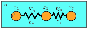
Figure 1: Elastic three-sphere microswimmer in a viscous fluid characterized by the shear viscosity $\eta$. Three identical spheres of radius $a$ are connected by two harmonic springs whose elastic constants are $K_{\rm A}$ and $K_{\rm B}$. The natural lengths of the springs, $\ell_{\rm A}(t)$ and $\ell_{\rm B}(t)$, depend on time and are assumed to undergo cyclic change [see Eqs. (6) and (7)]. The time-dependent positions of the spheres are denoted by $x_{1}(t)$, $x_{2}(t)$, and $x_{3}(t)$ in a one-dimensional coordinate.

In this letter, we discuss a generalized three-sphere swimmer in which the spheres are simply connected by two harmonic springs. The main difference compared with the previous models is that the natural length of each spring depends on time and is assumed to undergo a prescribed cyclic change. Whereas the arms in the Najafi–Golestanian model undergo a prescribed motion regardless of the force exerted by the fluid, the sphere motion in our model is determined by the natural spring lengths representing internal states of a swimmer, and also by the force exerted by the fluid. In this sense, our model is more realistic to study the locomotion of active microswimmers. We analytically obtain the average swimming velocity as a function of the frequency of the cyclic change in the natural length. In order to better illustrate our result, we first explain the case when the two spring constants are identical, and also the two oscillation amplitudes of the natural lengths are the same. Then we shall argue a general case when these quantities are different and when the phase mismatch between the natural lengths is arbitrary.

The introduction of harmonic springs between the spheres leads to an intrinsic time scale of an elastic swimmer that characterizes its internal relaxation dynamics. When the frequency of the cyclic change in the natural lengths is smaller than this characteristic time, the swimming velocity increases with the frequency as in the previous works Golestanian08 . In the high-frequency region, on the other hand, the motion of spheres cannot follow the change in the natural length, and the average swimming velocity decreases with increasing the frequency. Such a situation resembles to the dynamics of the Najafi–Golestanian three-sphere swimmer in a viscoelastic medium Yasuda17 . We also show that, due to the elasticity that has been introduced, the proposed micromachine can swim even if the change in the natural lengths is reciprocal as long as its structural symmetry is violated. Although the considered swimmer appears to be somewhat trivial, it can be regarded as a generic model for microswimmers or protein machines since the behaviors of the previous models can be deduced from our model by taking different limits.

We generalize the Najafi–Golestanian three-sphere swimmer model to take into account the elasticity in the sphere motion. As schematically shown in Fig. 1, the present model consists of three hard spheres of the same radius $a$ connected by two harmonic springs A and B whose spring constants are $K_{\rm A}$ and $K_{\rm B}$, respectively. We assume that the natural lengths of these springs, denoted by $\ell_{\rm A}(t)$ and $\ell_{\rm B}(t)$, undergo cyclic time-dependent change. Their explicit time dependences will be specified later. The total energy of an elastic swimmer is then given by

$$E=\frac{K_{\rm A}}{2}(x_{2}-x_{1}-\ell_{\rm A})^{2}+\frac{K_{\rm B}}{2}(x_{3}-x_{2}-\ell_{\rm B})^{2},$$ (1)

where $x_{i}(t)$ ($i=1,2,3$) are the positions of the three spheres in a one-dimensional coordinate. We also assume $x_{1}<x_{2}<x_{3}$ without loss of generality. Owing to the hydrodynamic interaction, each sphere exerts a force on the viscous fluid of shear viscosity $\eta$ and experiences an opposite force from it. In general, the surrounding medium can be viscoelastic Yasuda17 , but such an effect is not considered in this letter.

Denoting the velocity of each sphere by $\dot{x}_{i}$, we can write the equations of motion of the three spheres as

$$\dot{x}_{1} =\frac{K_{\rm A}}{6\pi\eta a}(x_{2}-x_{1}-\ell_{\rm A})-\frac{K_{\rm A}}{4\pi\eta}\frac{(x_{2}-x_{1}-\ell_{\rm A})}{x_{2}-x_{1}}+\frac{K_{\rm B}}{4\pi\eta}\frac{(x_{3}-x_{2}-\ell_{\rm B})}{x_{2}-x_{1}}-\frac{K_{\rm B}}{4\pi\eta}\frac{(x_{3}-x_{2}-\ell_{\rm B})}{x_{3}-x_{1}},$$ (2)

$$\dot{x}_{2} =\frac{K_{\rm A}}{4\pi\eta}\frac{(x_{2}-x_{1}-\ell_{\rm A})}{x_{2}-x_{1}}-\frac{K_{\rm A}}{6\pi\eta a}(x_{2}-x_{1}-\ell_{\rm A})+\frac{K_{\rm B}}{6\pi\eta a}(x_{3}-x_{2}-\ell_{\rm B})-\frac{K_{\rm B}}{4\pi\eta}\frac{(x_{3}-x_{2}-\ell_{\rm B})}{x_{3}-x_{2}},$$ (3)

$$\dot{x}_{3} =\frac{K_{\rm A}}{4\pi\eta}\frac{(x_{2}-x_{1}-\ell_{\rm A})}{x_{3}-x_{1}}-\frac{K_{\rm A}}{4\pi\eta}\frac{(x_{2}-x_{1}-\ell_{\rm A})}{x_{3}-x_{2}}+\frac{K_{\rm B}}{4\pi\eta}\frac{(x_{3}-x_{2}-\ell_{\rm B})}{x_{3}-x_{2}}-\frac{K_{\rm B}}{6\pi\eta a}(x_{3}-x_{2}-\ell_{\rm B}),$$ (4)

where we have used the Stokes’ law for a sphere and the Oseen tensor in a three-dimensional viscous fluid. The swimming velocity of the whole object can be obtained by averaging the velocities of the three spheres:

$$V=\frac{1}{3}(\dot{x}_{1}+\dot{x}_{2}+\dot{x}_{3}).$$ (5)

One of the advantages of the present formulation is that the motion of the spheres is simply described by coupled ordinary differential equations. Moreover, the force-free condition for the whole system Golestanian04 ; Golestanian08 is automatically satisfied in the above equations.

Next we assume that the two natural lengths of the springs undergo the following periodic changes:

$$\ell_{\rm A}(t) =\ell+d_{\rm A}\cos(\Omega t),$$ (6)

$$\ell_{\rm B}(t) =\ell+d_{\rm B}\cos(\Omega t-\phi).$$ (7)

In the above, $\ell$ is the common constant length, $d_{\rm A}$ and $d_{\rm B}$ are the amplitudes of the oscillatory change, $\Omega$ is the common frequency, and $\phi$ is the mismatch in the phases between the two cyclic changes. The time-reversal symmetry of the spring dynamics is present only when $\phi=0$ or $\pi$, otherwise the time-reversal symmetry is broken. In the following analysis, we generally assume that $d_{\rm A},d_{\rm B},a\ll\ell$ and focus on the leading order contribution. It is convenient to introduce a characteristic time scale $\tau=6\pi\eta a/K_{\rm A}$. Then we use $\ell$ to scale all the relevant lengths ($x_{i}$, $a$, $d_{\rm A}$, $d_{\rm B}$), and employ $\tau$ to scale the frequency, i.e., $\hat{\Omega}=\Omega\tau$. By further defining the ratio between the two spring constants as $\lambda=K_{\rm B}/K_{\rm A}$, the coupled Eqs. (2)–(4) can be made dimensionless.

In order to present the essential outcome of the present model, we shall first consider the simplest symmetric case, i.e., $\lambda=1$, $d_{\rm A}=d_{\rm B}=d$, and $\phi=\pi/2$. Hence Eq. (7) now reads $\ell_{\rm B}(t)=\ell+d\sin(\Omega t)$. For our later calculation, it is useful to introduce the following spring lengths with respect to $\ell$:

$$u_{\rm A}=x_{2}-x_{1}-\ell,~{}~{}~{}~{}~{}u_{\rm B}=x_{3}-x_{2}-\ell.$$ (8)

Notice that these quantities are related to the sphere velocities in Eqs. (2)–(4) as

$$\dot{u}_{\rm A}=\dot{x}_{2}-\dot{x}_{1},~{}~{}~{}~{}~{}\dot{u}_{\rm B}=\dot{x}_{3}-\dot{x}_{2}.$$ (9)

Using Eqs. (2)–(4) and solving Eq. (9) in the frequency domain, we obtain after the inverse Fourier transform as

$$u_{\rm A}(t) \approx\frac{9-3\hat{\Omega}+5\hat{\Omega}^{2}+\hat{\Omega}^{3}}{9+10\hat{\Omega}^{2}+\hat{\Omega}^{4}}d\cos(\Omega t)$$

$$+\frac{6\hat{\Omega}-4\hat{\Omega}^{2}+2\hat{\Omega}^{3}}{9+10\hat{\Omega}^{2}+\hat{\Omega}^{4}}d\sin(\Omega t),$$ (10)

$$u_{\rm B}(t) \approx-\frac{6\hat{\Omega}+4\hat{\Omega}^{2}+2\hat{\Omega}^{3}}{9+10\hat{\Omega}^{2}+\hat{\Omega}^{4}}d\cos(\Omega t)$$

$$+\frac{9+3\hat{\Omega}+5\hat{\Omega}^{2}-\hat{\Omega}^{3}}{9+10\hat{\Omega}^{2}+\hat{\Omega}^{4}}d\sin(\Omega t),$$ (11)

where we have used $a/\ell\ll 1$.

According to the calculation by Golestanian and Ajdari Golestanian08 , the average swimming velocity of a three-sphere swimmer can generally be expressed up to the leading order in $u_{\rm A}/\ell$ and $u_{\rm B}/\ell$ as

$$\overline{V}=\frac{7a}{24\ell^{2}}\langle u_{\rm A}\dot{u}_{\rm B}-\dot{u}_{\rm A}u_{\rm B}\rangle,$$ (12)

where the averaging $\langle\cdots\rangle$ is performed by time integration in a full cycle. The above expression indicates that the average velocity is determined by the area enclosed by the orbit of the periodic motion in the configuration space Golestanian08 . Using Eqs. (10) and (11) for an elastic microswimmer with $d/\ell,a/\ell\ll 1$, we obtain the lowest order contribution as

$$\overline{V}=\frac{7d^{2}a}{24\ell^{2}\tau}\frac{3\hat{\Omega}(3+\hat{\Omega}^{2})}{9+10\hat{\Omega}^{2}+\hat{\Omega}^{4}},$$ (13)

which is an important result of this letter.

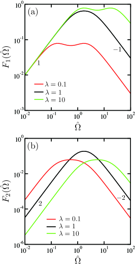
Figure 2: Plots of the scaling functions (a) $F_{1}(\hat{\Omega};\lambda)$ and (b) $F_{2}(\hat{\Omega};\lambda)$ defined in Eqs. (22) and (23), respectively, as a function of $\hat{\Omega}=\Omega\tau$ for $\lambda=K_{\rm B}/K_{\rm A}=0.1,1,$ and $10$. The numbers indicate the slope representing the exponent of the power-law behaviors.

We first consider the small-frequency limit of $\hat{\Omega}\ll 1$. Physically, this limit corresponds to the case when the spring constant $K_{\rm A}$ is very large. We easily obtain

$$u_{\rm A}(t)\approx d\cos(\Omega t),~{}~{}~{}~{}~{}u_{\rm B}(t)\approx d\sin(\Omega t),$$ (14)

and

$$\overline{V}\approx\frac{7d^{2}a\Omega}{24\ell^{2}},$$ (15)

which exactly coincides with the average velocity of the Najafi-Golestanian swimmer with equal spheres Golestanian04 ; Golestanian08 . This is reasonable because the two spring lengths $u_{\rm A}$ and $u_{\rm B}$ are in phase with their respective natural lengths $\ell_{\rm A}$ and $\ell_{\rm B}$, as we see from Eqs. (6), (7), and (14). Notice that the average velocity increases as $\overline{V}\sim\Omega$ in this limit, while it does not depend on the fluid viscosity $\eta$ Golestanian04 ; Golestanian08 .

In the opposite large-frequency limit of $\hat{\Omega}\gg 1$, on the other hand, we have

$$u_{\rm A}(t) \approx\frac{\sqrt{5}d}{\Omega\tau}\cos[\Omega t-\arctan 2],$$ (16)

$$u_{\rm B}(t) \approx\frac{\sqrt{5}d}{\Omega\tau}\sin[\Omega t-(\pi-\arctan 2)],$$ (17)

where $\arctan 2\approx 1.107$ and

$$\overline{V}\approx\frac{21d^{2}a}{24\ell^{2}\Omega\tau^{2}}.$$ (18)

We see here that $u_{\rm A}$ and $u_{\rm B}$ are out of phase with respect to the natural lengths $\ell_{\rm A}$ and $\ell_{\rm B}$, while the average velocity decreases as $\overline{V}\sim\Omega^{-1}$ when $\Omega$ is increased. When the spring constant $K_{\rm A}$ is small, it takes time for a spring to relax to its natural length, which leads to a delay in the mechanical response. The crossover frequency between the above two regimes is determined by $\hat{\Omega}\sim 1$. The general frequency dependence of Eq. (13) is shown in Fig. 2(a) for $\lambda=1$ (black line). It shows a maximum around $\hat{\Omega}\sim 1$, as expected.

Recently, we have investigated the motion of the Najafi-Golestanian three-sphere swimmer in a viscoelastic medium Yasuda17 . We derived a relation that connects the average swimming velocity and the frequency-dependent viscosity of the surrounding medium. In this relation, the viscous contribution can exist only when the time-reversal symmetry is broken, whereas the elastic contribution is present only when the structural symmetry of the swimmer is broken. In particular, we calculated the average swimming velocity when the surrounding viscoelastic medium is described by a simple Maxwell fluid with a characteristic time scale $\tau_{\rm M}$. It was show that the viscous term increases as $\overline{V}\sim\Omega$ for $\Omega\tau_{\rm M}\ll 1$, while it decreases as $\overline{V}\sim\Omega^{-1}$ for $\Omega\tau_{\rm M}\gg 1$. This is a unique feature of a swimmer in a viscoelastic medium Yasuda17 ; Lauga09 ; Curtis13 , and such a reduction occurs simply because the medium responds elastically in the high-frequency regime. We note that the frequency dependence of $\overline{V}$ for an elastic three-sphere swimmer, as obtained in Eqs. (13), is analogous to the Najafi-Golestanian swimmer in a Maxwell fluid. In other words, an elastic microswimmer in a viscous fluid exhibits “viscoelastic” effects as a whole.

Having discussed the simplest situation of the proposed elastic swimmer, we now show the result for a general case when $K_{\rm A}\neq K_{\rm B}$ (or $\lambda\neq 1$), $d_{\rm A}\neq d_{\rm B}$ and the phase mismatch $\phi$ in Eq. (7) is arbitrary. By repeating the same calculation as before, the spring lengths in Eq. (8) now become

$$u_{\rm A}(t)\approx \frac{1}{9\lambda^{2}+2(2+\lambda+2\lambda^{2})\hat{\Omega}^{2}+\hat{\Omega}^{4}}$$

$$\times \biggl{\{}[9\lambda^{2}+(4+\lambda)\hat{\Omega}^{2}]d_{\rm A}\cos(\Omega t)$$

$$+2(3\lambda^{2}+\hat{\Omega}^{2})\hat{\Omega}d_{\rm A}\sin(\Omega t)$$

$$-2\lambda(1+\lambda)\hat{\Omega}^{2}d_{\rm B}\cos(\Omega t-\phi)$$

$$-\lambda(-3\lambda+\hat{\Omega}^{2})\hat{\Omega}d_{\rm B}\sin(\Omega t-\phi)\biggr{\}},$$ (19)

$$u_{\rm B}(t)\approx \frac{1}{9\lambda^{2}+2(2+\lambda+2\lambda^{2})\hat{\Omega}^{2}+\hat{\Omega}^{4}}$$

$$\times \biggl{\{}-2(1+\lambda)\hat{\Omega}^{2}d_{\rm A}\cos(\Omega t)$$

$$+(3\lambda-\hat{\Omega}^{2})\hat{\Omega}d_{\rm A}\sin(\Omega t)$$

$$+\lambda[9\lambda+(1+4\lambda)\hat{\Omega}^{2}]d_{\rm B}\cos(\Omega t-\phi)$$

$$+2\lambda(3+\hat{\Omega}^{2})\hat{\Omega}d_{\rm B}\sin(\Omega t-\phi)\biggr{\}},$$ (20)

respectively, where we have used $a/\ell\ll 1$. Using again Eq. (12), we finally obtain the lowest order general expression of the average velocity as

$$\overline{V} =\frac{7d_{\rm A}d_{\rm B}a}{24\ell^{2}\tau}F_{1}(\hat{\Omega};\lambda)\sin\phi$$

$$-\frac{7(\lambda-1)d_{\rm A}d_{\rm B}a}{12\ell^{2}\tau}F_{2}(\hat{\Omega};\lambda)\cos\phi$$

$$+\frac{7(d_{\rm A}^{2}-d_{\rm B}^{2}\lambda)a}{24\ell^{2}\tau}F_{2}(\hat{\Omega};\lambda),$$ (21)

where the two scaling functions are defined by

$$F_{1}(\hat{\Omega};\lambda) =\frac{3\lambda\hat{\Omega}(3\lambda+\hat{\Omega}^{2})}{9\lambda^{2}+2(2+\lambda+2\lambda^{2})\hat{\Omega}^{2}+\hat{\Omega}^{4}},$$ (22)

$$F_{2}(\hat{\Omega};\lambda) =\frac{3\lambda\hat{\Omega}^{2}}{9\lambda^{2}+2(2+\lambda+2\lambda^{2})\hat{\Omega}^{2}+\hat{\Omega}^{4}}.$$ (23)

In Fig. 2, we plot the above scaling functions as a function of $\hat{\Omega}$ for different $\lambda$ values.

When $\lambda=1$, $d_{\rm A}=d_{\rm B}$, and $\phi=\pi/2$, only the first term remains, and Eq. (21) reduces to Eq. (13) as it should. When $\lambda\neq 1$, on the other hand, the second term is present even if $\phi=0$. The third term is also present when $d_{\rm A}^{2}\neq d_{\rm B}^{2}\lambda$ regardless of the phase mismatch $\phi$. Notice that both the second and the third terms reflect the structural asymmetry of an elastic three-sphere swimmer, whereas the first term represents the broken time-reversal symmetry for $\phi\neq 0$ Yasuda17 . It is interesting to note that the frequency dependence of the second and the third terms in Eq. (21), represented by $F_{2}(\hat{\Omega},\lambda)$, is different from that of the first term, represented by $F_{1}(\hat{\Omega},\lambda)$. According to Eq. (23), $\overline{V}$ due to the second and the third terms increases as $\overline{V}\sim\Omega^{2}$ for $\hat{\Omega}\ll 1$, whereas it decreases as $\overline{V}\sim\Omega^{-2}$ for $\hat{\Omega}\gg 1$. In general, the overall swimming velocity depends on various structural parameters and exhibits a complex frequency dependence. For example, we point out that $F_{1}(\hat{\Omega},\lambda)$ in Fig. 2(a) exhibits non-monotonic frequency dependence (two maxima) for $\lambda=0.1$ or $10$ (namely, when $\lambda\neq 1$). On the other hand, an important common feature in all the terms in Eq. (21) is that $\overline{V}$ decreases for $\hat{\Omega}\geq 1$, which is characteristic for elastic swimmers.

We confirm again that Eq. (21) reduces to the result by Golestanian and Ajdari Golestanian08 , i.e., $\overline{V}=7d_{\rm A}d_{\rm B}a\Omega\sin\phi/(24\ell^{2})$, when the two spring constants are infinitely large $K_{\rm A},K_{\rm B}\rightarrow\infty$ and $\lambda=1$. The third term in Eq. (21) vanishes even if $d_{\rm A}\neq d_{\rm B}$ because $\hat{\Omega}\rightarrow 0$ holds in this limit. In the modified three-sphere swimmer model considered by Montino and DeSimone, one of the two arms was replaced by a passive elastic spring Montino15 . Their model can be obtained from the present model simply by setting one of the spring constants to be infinitely large, say $K_{\rm A}\rightarrow\infty$, and by regarding the natural length of the other spring as a constant, say $\ell_{\rm B}=\ell$ (or $d_{\rm B}=0$). The continuous changes of the natural lengths introduced in Eqs. (6) and (7) are straightforward generalization of cyclically switched discrete states considered in the previous studies GolestanianAjdari08 ; Golestanian10 ; Sakaue10 ; Huang12 . We finally note that a similar model to the present one was considered in Ref. Dunkel09 , although they focused only in the small-frequency region and did not discuss the entire frequency dependence. Using coupled Langevin equations, they mainly investigated the interplay between self-driven motion and diffusive behavior Dunkel09 , which is also an important aspect of microswimmers.

To summarize, we have discusses the locomotion of a generalized three-sphere microswimmer in which the spheres are connected by two elastic springs and the natural length of each spring is assumed to undergo a prescribed cyclic change. As shown in Eqs. (13) and (21), we have analytically obtained the average swimming velocity $\overline{V}$ as a function of the frequency $\Omega$ of the cyclic change in the natural length. In the low-frequency region, the swimming velocity increases with the frequency and reduces to the original three-sphere model by Najafi and Golestanian Golestanian04 ; Golestanian08 . In the high-frequency region, conversely,, the velocity is a decreasing function. This property reflects the intrinsic spring relaxation dynamics of an elastic swimmer in a viscous fluid.

S.K. and R.O. acknowledge support from a Grant-in-Aid for Scientific Research on Innovative Areas “Fluctuation and Structure” (Grant No. 25103010) from the Ministry of Education, Culture, Sports, Science, and Technology of Japan and from a Grant-in-Aid for Scientific Research (C) (Grant No. 15K05250) from the Japan Society for the Promotion of Science (JSPS).

References

- (1) E. Lauga and T. R. Powers, Rep. Prog. Phys. 72 096601 (2009).
- (2) E. M. Purcell, Am. J. Phys. 45, 3 (1977).
- (3) E. Lauga, Soft Matter 7, 3060 (2011).
- (4) A. Najafi and R. Golestanian, Phys. Rev. E 69, 062901 (2004).
- (5) R. Golestanian and A. Ajdari, Phys. Rev. E 77, 036308 (2008).
- (6) G. Grosjean, M. Hubert, G. Lagubeau, and N. Vandewalle, Phys. Rev. E 94, 021101(R) (2016).
- (7) R. Golestanian, Eur. Phys. J. E 25, 1 (2008).
- (8) R. Ledesma-Aguilar, H. Löwen, and J. M. Yeomans, Eur. Phys. J. E 35, 70 (2012).
- (9) A. Montino and A. DeSimone, Eur. Phys. J. E 42, 38 (2015).
- (10) A. Montino and A. DeSimone, Acta Appl. Math. 149, 53 (2017).
- (11) R. Golestanian and A. Ajdari, Phys. Rev. Lett. 100, 038101 (2008).
- (12) R. Golestanian, Phys. Rev. Lett. 105, 018103 (2010).
- (13) T. Sakaue, R. Kapral, and A. S. Mikhailov, Eur. Phys. J. B 75, 381 (2010).
- (14) M.-J. Huang, H.-Y. Chen, and A. S. Mikhailov, Eur. Phys. J. E 119, 35 (2012).
- (15) K. Yasuda, R. Okamoto, and S. Komura, J. Phys. Soc. Jpn. 86, 043801 (2017).
- (16) E. Lauga, EPL 86, 64001 (2009).
- (17) M. P. Curtis and E. A. Gaffney, Phys. Rev. E 87, 043006 (2013).
- (18) J. Dunkel and I. M. Zaid, Phys. Rev. E 80, 021903 (2009).