A Helicity-Based Method to Infer the CME Magnetic Field Magnitude in Sun and Geospace: Generalization and Extension to Sun-Like/M-Dwarf Stars and Implications for Exoplanet Habitability

1 Introduction

Knowledge of the magnetic field of coronal mass ejections (CMEs), both near the Sun, and further away at 1 AU, is a key parameter toward understanding their structure, evolution, energetics, and geoeffectiveness. For example, the energy stored in non-potential CME magnetic fields is more than sufficient to counterbalance their mechanical energy (e.g. Forbes, 2000; Vourlidas et al., 2000). In addition, the magnitude of the southward interplanetary (IP) magnetic field associated with CMEs reaching 1 AU is arguably the most important parameter for determining the magnitude of the associated geomagnetic storms (e.g. Wu and Lepping, 2005). In stellar obsevations, the recent detections of superflares with energies of up to $10^{4}$ times the energy of “typical” solar flares, on Sun-like stars (e.g. Maehara et al., 2012; Shibayama et al., 2013), and their possible association with stellar CMEs, may have significant implications for the physical conditions and the eventual habitability of exoplanets orbiting super-flaring stars (e.g. Khodachenko et al., 2007; Lammer et al., 2007; Vidotto et al., 2013; Armstrong et al., 2016; Kay, Opher, and Kornbleuth, 2016). The stellar CME magnetic field at exoplanet orbit is an important parameter for its habitability since it enters into the calculation of the exoplanet magnetosphere size.

Unfortunately, few direct determinations of near-Sun CME magnetic fields currently exist, not to mention stellar CMEs, (e.g. Bastian et al., 2001; Jensen and Russell, 2008; Tun and Vourlidas, 2013; Hariharan et al., 2016; Howard et al., 2016; Kooi et al., 2016). These determinations occur from non-routine, exceptional observations in the radio domain (e.g. Faraday rotation, moving type IV bursts).

In parallel, methods for CME magnetic field inference have emerged (Kunkel and Chen, 2010; Savani et al., 2015). We have recently developed a novel method to infer the near-Sun and 1 AU magnetic field magnitude. For the remainder of this article, and for brevity, by CME magnetic field we will mean CME magnetic field magnitude. (Patsourakos et al., 2016; Patsourakos and Georgoulis, 2016). In a nutshell, our method is based on the principle of magnetic helicity conservation applied to CMEs. It uses analytical relationships connecting the CME magnetic field with its magnetic helicity $H_{\textrm{m}}$, and a set of its geometrical parameters (e.g. CME length, radius). Magnetic helicity is a signed quantity, depending on its handedness. For the remainder of this article, and for brevity, when referring to magnetic helicity we will refer to its magnitude.

CME magnetic helicity and geometrical parameters can be routinely deduced from photospheric and coronal observations, respectively. Invoking the magnetic helicity conservation property (e.g. Berger, 1984), therefore, allows to infer the CME near-Sun magnetic field. Finally, radial power-law extrapolation of the inferred near-Sun CME magnetic field allows to calculate its value at 1 AU. We applied our method to an observed case-study in Patsourakos et al. (2016), corresponding to a super-fast CME which gave rise to one of the most intense geomagnetic storms of Solar Cycle 24. In Patsourakos and Georgoulis (2016) we performed a parametric study of our method, based on the observed distributions of its input parameters (CME magnetic helicity and geometrical parameters). We used one of the most common flux-rope CME models (Lundquist 1950).

In the present study we extend our initial work in two meaningful ways: first, we generalize our parametric study on an array of proposed theoretical CME models, thereby further constraining the radial field evolution of the modeled CMEs in the interplanetary medium (Sections 2 and 3). Second, we extend our framework to non-solar cases, particularly to stars hosting superflares, and determine the magnetic fields of possible stellar CMEs associated with these extreme events. This allows us to infer some rough limits on magnetosphere size of exoplanets orbiting such stars and to cast some preliminary implications for their habitability (Section 4). We conclude with a summary and a discussion of our results, as well as possible avenues for future research (Section 5).

2 The Helicity-Based Method to Infer the Near-Sun and 1 AU CME Magnetic FIeld

We briefly describe here our framework for inferring the near-Sun and 1 AU magnetic field of CMEs, in Sections 2.1 and 2.2, respectively, and its parametrization, in Section 2.3. More details can be found in Patsourakos et al. (2016) and Patsourakos and Georgoulis (2016).

2.1 Determination of CME Near-Sun Magnetic Field

First, we infer the near-Sun CME magnetic field as follows:

1. Determine the magnetic helicity $H_{\textrm{m}}$ of the CME solar source region using various methods based on theory and photospheric observations (Pariat et al., 2006; Régnier and Canfield, 2006; Georgoulis, Tziotziou, and Raouafi, 2012; Valori, Démoulin, and Pariat, 2012; Moraitis et al., 2014, among others).

2. Attribute the source-region $H_{\textrm{m}}$ to the analyzed CME.

3. Determine a set of CME geometrical parameters (e.g. radius $R$, length $L$) from forward-modeling geometrical fits of multi-view coronal observations of the analyzed CME (Section A of Appendix). Such observations are achieved by coronagraphs typically covering the outer corona.

4. Plug the magnetic and geometrical parameters of the CME deduced in the previous two steps into theoretical formulations, such as the models described in Sections B-G of Appendix, and deduce the corresponding near-Sun magnetic field magnetic field $B_{*}$ at heliocentric distance $r_{*}$.

2.2 Extrapolation of Near-Sun CME Magnetic Field to 1 AU

Next, we extrapolate $B_{*}$ from $r_{*}$, where coronagraphic observations of the CME geometrical properties are taken, outward in the IP space and eventually to 1 AU. We assume that its radial evolution is described by a power-law in the heliocentric radial distance $r$:

$$B_{0}(r)=B_{*}{(r/r_{*})}^{{\alpha}_{B}}.\ilabel{eq:scaleb}$$ (1)

In Equation (eq:scaleb) we assume that the power-law index ${\alpha}_{B}$ varies in the range [-2.7, -1.0]. This results from various theoretical and observational studies (e.g. Patzold et al., 1987; Kumar and Rust, 1996; Bothmer and Schwenn, 1998; Vršnak, Magdalenić, and Zlobec, 2004; Liu, Richardson, and Belcher, 2005; Forsyth et al., 2006; Leitner et al., 2007; Démoulin and Dasso, 2009; Möstl et al., 2012; Poomvises et al., 2012; Mancuso and Garzelli, 2013; Good et al., 2015; Winslow et al., 2015). Notice here that most of these studies do not fully cover the range we are considering here, but typically subsets thereof, either near-Sun or inner heliospheric. We considered 18 equidistant ${\alpha}_{B}$-values and a step of 0.1. In Patsourakos et al. (2016) we applied our method to an observed super-fast CME which gave rise to one of the most intense geomagnetic storms of Solar Cycle 24. We found that a rather steep CME magnetic field evolution of the inferred near-Sun CME magnetic magnetic field in the IP space, with an index ${\alpha}_{B}\simeq-2$, was consistent with the range of the associated interplanerary CME (ICME) magnetic field values as observed in-situ at $\approx$1 AU (i.e. at the L1 Lagrangian libration point).

2.3 Parametric Study of the Helicity-Based Method

In Patsourakos and Georgoulis (2016) we performed a parametric study of our method. We carried out Monte-Carlo simulations of ${10}^{4}$ synthetic CMEs and used the frequently-used Lundquist model (Section B of Appendix). Our simulations randomly sampled ${10}^{4}$ values of active region (AR) $H_{\textrm{m}}$, CME aspect ratio $k$ and angular half-width $w$ from the observed distributions of 42 ARs (Tziotziou, Georgoulis, and Raouafi, 2012) and 65 CMEs (Thernisien, Vourlidas, and Howard, 2009; Bosman et al., 2012), respectively. Using the randomly selected CME aspect ratio and angular half-width in Equations (eq:cmer) and (eq:cmelength), the CME radius and length, respectively, were deduced, and finally, the CME magnetic field was determined via Equations (eq:hm) and (eq:alpha). As a result, $10^{4}$ $B_{*}$ values at $r_{*}=10\,\mathrm{R_{\odot}}$ were calculated. These near-Sun magnetic fields were then extrapolated to 1 AU, therefore leading to 180,000 1 AU CME magnetic field values, resulting from the matrix of ${10}^{4}$ $B_{*}$ and 18 ${\alpha}_{B}$ values discussed in Sections 2.1 and 2.2. We found that an index ${\alpha}_{B}$ = -1.6 $\pm 0.2$ led to a ballpark, statistical agreement between the model-predicted ICME magnetic field distributions and actual ICME observations at 1 AU.

3 Parametric Study of the Helicity-Based Method for Different CME Models

In this Section we extend and generalize the parametric study of Patsourakos and Georgoulis (2016) to six different CME models, including the Lundquist model used in that study. These models, described in Sections B-G of Appendix, make different assumptions about the CME shape (cylindrical segment, toroidal, spheromac), the nature of their currents (linear/nonlinear force-free, non force-free) and the distribution of twist (uniform, non-uniform), thereby allowing maximum flexibility in our method’s application.

As in Patsourakos and Georgoulis (2016), we perform Monte-Carlo simulations picking up ${10}^{4}$ random deviates from the observed distributions of the input magnetic ($H_{\textrm{m}}$) and geometrical ($k$ and $w$) parameters of our method and determine ${10}^{4}B_{*}$ values for each considered model using the corresponding equations per model (Sections B-G of Appendix). Depending on the specific model assumptions, extra geometrical parameters are used (e.g. CME minor and major radius in Equation (9); number of turns in Equations (11) and (13)). For each considered model we calculate the probability density function (PDF) of: (1) the extrapolated to 1 AU CME magnetic fields, ${w{B}_{\textrm{1 AU}}}$, for the ${10}^{4}$ $B_{*}$ values and for each of the 18 considered ${\alpha}_{B}$ values, $\textrm{{PDF}}_{\textrm{mod}}$; and (2) the magnetic fields, $B_{\textrm{MC}}$, for 162 magnetic clouds (MCs) observed at 1 AU as resulting from their linear force-free fits (Lynch et al., 2003; Lepping et al., 2006), and $\textrm{{PDF}}_{\textrm{obs}}$.

We compare the results of our Monte-Carlo simulations for the six different employed models with MC observations in Figures fig:fig1 and fig:fig2. In Figure fig:fig1 we display the correlation coefficient of $\textrm{{PDF}}_{\textrm{mod}}$ and $\textrm{{PDF}}_{\textrm{obs}}$ as a function of ${\alpha}_{\textrm{B}}$, whereas in Figure fig:fig2 we diplay the fraction $\textrm{{frac}}_{\textrm{MC}}$ of ${B_{\textrm{1 AU}}}$ values falling within the observed $B_{\textrm{MC}}$ range, namely [4,45] nT, as a function of ${\alpha}_{B}$.

Several remarks can be now made:

1. Both $\rm{{PDF}}_{\textrm{mod}}$ versus $\rm{{PDF}}_{\textrm{obs}}$ correlation coefficients and $\textrm{{frac}}_{\textrm{MC}}$ exhibit well-defined peaks, and cover similar ${\alpha}_{B}$-ranges of $\approx$ [-1.85, -1.2] and [-2.0,-1.3], respectively, for all considered models. For the cases of the toroidal and spheromak linear force-free models there are secondary peaks for ${\alpha}_{B}<-2$ (Figure fig:fig1). However these peaks are not supported by high $\textrm{{frac}}_{\textrm{MC}}$-values.

2. Similar (relatively high) peak values can be found in both Figures fig:fig1 ($\approx$ 0.9) and fig:fig2 ($\approx$ 0.7) for all considered models. The full width at half maximum (FWHM) of the curves of Figures fig:fig1 and fig:fig2 is $\approx$ [0.3,0.5] and [0.7,0.8], respectively, in the ${\alpha}_{\textrm{B}}$-range.

3. The linear and nonlinear force-free, cylindrical, flux-rope models, black and red lines, respectively, in both Figures fig:fig1 and fig:fig2, place the median of the considered models.

Figure fig:fig3 displays the model-averaged $\textrm{{PDF}}_{\textrm{mod}}$ versus $\textrm{{PDF}}_{\textrm{obs}}$ correlation coefficient and $\textrm{{frac}}_{\textrm{MC}}$ as a function of ${\alpha}_{B}$. These plots encapsulate the overall performance of all considered models. The corresponding curves peak at ${\alpha}_{B}\approx-1.6$ and ${\alpha}_{B}\approx-1.8$ for the $\textrm{{PDF}}_{\textrm{mod}}$ versus $\textrm{{PDF}}_{\textrm{obs}}$ correlation coefficient and $\textrm{{frac}}_{\textrm{MC}}$, respectively. Both peaks correspond to relatively high values of $\approx$0.6.

4 Extension to Stellar CMEs

Existing stellar observations lack the spatial resolution to directly image possible stellar CMEs, not to mention their source regions. Therefore, we have to rely on indirect observational inferences for stellar CMEs (e.g. Houdebine, Foing, and Rodono, 1990; Leitzinger et al., 2011; Osten et al., 2013; Leitzinger et al., 2014). Solar observations suggest that with increasing flare magnitude, the probability of an associated CME is also increasing, with GOES-class flares $\gtrsim$X3 essentially associated one-to-one to fast or superfast CMEs (e.g. Andrews, 2003; Yashiro et al., 2005; Nindos et al., 2015; Harra et al., 2016). Therefore, it is possible that stars with superflares could have enhanced rates of superfast CMEs associated to them. Stars hosting superflares are generally characterized by enhanced magnetic activity, as inferred from their larger chromospheric emissions (e.g. Karoff et al., 2016). A common practice in studies of stellar flares and CMEs is to extrapolate empirical relationships derived from solar studies to the stellar context (e.g. Aarnio, Matt, and Stassun, 2012; Drake et al., 2013; Osten and Wolk, 2015).

Therefore, in order to determine the $H_{\textrm{m}}$ associated with stellar CMEs, we rely on a recently discovered empirical relationship connecting the free coronal magnetic energy $E_{\textrm{f}}$ and $H_{\textrm{m}}$ of solar active regions. Tziotziou, Georgoulis, and Raouafi (2012) inferred the following best fit for 42 solar ARs and 162 snapshots thereof:

$$\textrm{log}|H_{\textrm{m}}|=53.4-0.0524{(\textrm{log}(E_{\textrm{f}}))^{0.653}}\textrm{exp}(\frac{97.45}{\textrm{log}(E_{\textrm{f}})}).\ilabel{eq:hmefree}$$ (2)

Equation (eq:hmefree) was applied to an $\rm{E_{f}}$ interval of ${10}^{30}-{10}^{33}\mathrm{erg}$. We consider stellar eruptive flares (i.e. assosiated with stellar CMEs) with energies in the range ${10}^{32}-10^{36}\mathrm{erg}$, and cover this interval with a logarithmic step of 0.1 leading to 41(=$N_{E_{\textrm{f}}}$) bins in $E_{\textrm{f}}$. The employed interval includes both solar flares and stellar superflares (e.g. Shibayama et al., 2013); stellar superflares have a most probable energy of few times ${10}^{34}$ erg. Notice that typically the quoted superflare energies are bolometric, i.e. correspond to the wavelength-integrated radiated energy (e.g. Maehara et al., 2012; Shibayama et al., 2013). For each considered flare energy we assume an equal free magnetic energy. This assumption imposes a lower limit on the free magnetic energy of the host active region, since we know that the largest flare in an active region releases a relatively small percentage (typically 10 – 20 %) of the free magnetic energy stored in the region (e.g. Lynch et al., 2008; Sun et al., 2012; Tziotziou, Georgoulis, and Raouafi, 2012; Tziotziou, Georgoulis, and Liu, 2013).

Having determined the magnetic helicities that could be associated with stellar CMEs, we then adopt typical values for $k$ (=0.3) and $w$ (=20 degrees) as resulting from solar studies of CMEs (e.g. Thernisien, Vourlidas, and Howard, 2009; Bosman et al., 2012) and determine their near-star stellar CME magnetic field values at 10 $\mathrm{R_{\odot}}$ by applying the Lundquist model (Section B of Appendix). Next, adopting the radial power-law CME magnetic field evolution of Equation (eq:scaleb), we extrapolate the derived near-star stellar CME magnetic fields in the range [0.05,1.5] AU, which spans the habitable zone (HZ) of exoplanet candidates (Kane et al., 2016). HZ is typically defined as the distance from a mother star at which water could exist in a liquid form (e.g. Kasting, Whitmire, and Reynolds, 1993; Selsis et al., 2007; Khodachenko et al., 2007). This obviously corresponds to a minimum requirement for life-sustaining conditions in exoplanets. The HZ migrates closer to the mother star when moving from Sun-like stars to M-dwarfs (e.g. see Figure 3 in Selsis et al., 2007).

We cover the above-mentioned radial distance interval with a radial step of 0.003 AU, leading to 480($=N_{r}$) bins in radial distance. We assume that this interval is populated with exoplanets having a magnetosphere. For the extrapolation we employ an index ${\alpha}_{B}=-1.6$ since it corresponds to the “best-fit” for the Lundquist model for the solar-terestrial case (Patsourakos and Georgoulis, 2016). We therefore calculate a two-dimensional, $41\times 480$ $N_{\textrm{{r}}}$ versus $N_{E_{\textrm{{f}}}}$ grid of extrapolated stellar CME magnetic fields, at the locations of hypothetical exoplanets and for the employed stellar flare energies. We finally determine the magnetopause radius of hypothetical exoplanets at the considered distance from a pressure-balance equation, balancing the stellar CME magnetic pressure at the exoplanet’s vicinity with the magnetic pressure of the intrinsic, assumed dipolar, planetary magnetic field (e.g. Chapman and Ferraro, 1930):

$$\frac{B_{\textrm{CME}}^{2}}{8\pi}=\frac{B_{\textrm{eq}}^{2}}{8\pi}{(\frac{1}{r_{\textrm{mpause}}})}^{6}.\ilabel{eq:mpause}$$ (3)

In Equation (eq:mpause), $B_{\textrm{CME}}$ is the extrapolated stellar CME magnetic field at the vicinity of the exoplanet, $B_{\textrm{eq}}$ is the planetary equatorial magnetic field, and $r_{\textrm{mpause}}$ is the magnetopause radius, assumed a dimensionless number in planetary radius ($R_{\textrm{p}}$) units. In writing Equation (eq:mpause) we assume a spherical magnetosphere. Given CMEs are magnetically-dominated structures, neglecting their thermal and ram pressure in Equation (eq:mpause) can be justified.

In Figure fig:fig4 we depict a color representation of the exoplanet magnetopause radius as a function of exoplanet distance and stellar flare magnitude. Given that current knowledge of magnetic fields in exoplanets is incomplete, we first assume that $B_{\textrm{eq}}$ is equal to the (current-day) terrestrial equatorial magnetic field ($B_{\textrm{E}}$=0.333 G). Values of $r_{\textrm{mpause}}$ smaller than 2 $R_{\textrm{p}}$ are saturated with black. This threshold corresponds to the minimum magnetosphere size that could prevent atmospheric erosion from stellar CME impacts (Khodachenko et al., 2007; Lammer et al., 2007; Scalo et al., 2007) and may be viewed as an additional, necessary condition for habitability. The maximum $r_{\textrm{mpause}}$ is $\approx 10R_{\textrm{p}}$, close to the unperturbed value for the terrestrial magnetosphere. From Figure fig:fig4 we notice that for exoplanets at distances $\lesssim$ 0.1 AU, practically all considered flare energies lead to magnetospheric compression below the 2 $R_{\textrm{p}}$ “habitability threshold” discussed above. Exoplanets at distances $\gtrsim$ 0.4 AU have $r_{\textrm{mpause}}\gtrsim 2R_{\textrm{p}}$ for all considered flare energies.

Moreover, exoplanets that are relatively close to their mother star could be subject to tidal locking, i.e. synchronization between their rotational and orbital periods, and generally a decrease in their rotation rate (e.g. Gladman et al., 1996). Slowing-down of an exoplanet leads to a decrease of its magnetic field (e.g. Grießmeier et al., 2004, 2005). In Figures fig:fig5 and fig:fig6 we calculated $r_{\textrm{mpause}}$ for two more cases, $B_{\textrm{eq}}=0.25B_{\textrm{E}}$ and $B_{\textrm{eq}}=0.061B_{\textrm{E}}$, respectively. These values correspond to calculations of planetary magnetic moments of Earth-like exoplanets in the close vicinity of M-type dwarf stars subject to tidal-locking (Khodachenko et al., 2007). The maximum $r_{\textrm{mpause}}$ is $\approx 6R_{\textrm{p}}$ and $\approx 4R_{\textrm{p}}$, for Figure fig:fig5 and fig:fig6, respectively. Decrease of the exoplanet magnetic field leads to further compression of its magnetopause radius for a given stellar flare energy, with exoplanets at distances $\lesssim$ 0.2 and $\lesssim$ 0.4 AU, for 0.25 $B_{\textrm{E}}$ and 0.061 $B_{\textrm{E}}$, respectively, with $r_{\textrm{mpause}}<2R_{\textrm{p}}$. In the case corresponding to 0.25 $B_{\textrm{E}}$ (Figure fig:fig5) exoplanets at distances $\gtrsim$ 1 AU have $r_{\textrm{mpause}}>2R_{p}$ for all considered flare energies. Moreover, in the case corresponding to 0.061 $B_{\textrm{E}}$ (Figure fig:fig6), only stellar flares with energies up ten times the lower limit ($={10}^{33}$ erg) of superflares could result in $r_{\textrm{mpause}}>2R_{\textrm{p}}$ for exoplanets at distances $\gtrsim$ 0.7 AU. Exoplanets at 1 AU experience magnetospheric compression below 2 $R_{\textrm{p}}$ only in the case of the smallest considered exoplanet magnetic field resulting from tidal locking (Figure fig:fig6).

Figures fig:fig4 – fig:fig6 include two case-studies of recently detected exoplanets orbiting stars hosting superflares. These are Kepler 438b (Torres et al., 2015; Armstrong et al., 2016) and Proxima b (Anglada-Escudé et al., 2016; Davenport et al., 2016), orbiting M-type dwarfs Kepler 438 and Proxima Centauri, respectively. Kepler 438b (Proxima b) have orbits with semi-major axis of 0.16 (0.04) AU and their mother stars exhibit superflares with energies 1.4$\times{10}^{33}$ (${10}^{33}$) erg. Kepler 438b and Proxima b have the highest Earth Similarity Index (ESI), 0.88 and 0.87, respectively, amongst the detected exoplanets to date. The ESI of a given exoplanet is a metric of its degree of resemblance with Earth in terms of mass, radius etc. An ESI equal to 1 suggests a perfect match of the exoplanet with Earth. From Figures fig:fig4 – fig:fig6 we gather that for all considered stellar flare energies and planetary magnetic fields, the hypothesized stellar CMEs result in severe magnetospheric compression, below $2R_{\textrm{p}}$ for both Kepler 438b and Proxima b. This appears to be a strong constraint against habitability of these exoplanets.

We finally investigate the effect of CMEs associated with potential solar superflares on the terrestrial magnetosphere. Based on our current understanding of solar dynamo and magnetic fields, geological and historical records, and super-flares observed in Sun-like stars one may not exclude the rare (i.e. over timescales of several centuries or more) occurrence of relatively small superflares (energies of up to $\approx{10}^{34}$) on the Sun (e.g. Shibata et al., 2013; Usoskin et al., 2013; Nogami et al., 2014; Toriumi et al., 2017), although such possibility has been contested (e.g. Schrijver et al., 2012; Aulanier et al., 2013; Cliver et al., 2014). Inspection of Figure fig:fig4, more specifically by considering a vertical cut at a distance equal to 1 AU, shows that solar superflares with energies exceeding ${10}^{33}$ and ${10}^{34}$ $\mathrm{erg}$ could lead to significant compression of the terrestrial magnetosphere at $\approx$ 6 and 5 Earth radii, respectively, in the case $\alpha_{B}=-1.6$ (Figure fig:fig7). For a steeper index $\alpha_{B}=-1.9$, the magnetopause distance stays above 6 Earth radii for a superflare with energy ${10}^{34}$ $\mathrm{erg}$ (Figure fig:fig8). Importantly, in no case does the magnetopause distance become smaller than 2 Earth radii, even for a “worst-case” superflare with energy ${10}^{36}$ erg.

5 Discussion and Conclusions

5.1 Summary of our Findings and Outlook

In this work, we (a) perform a parametric study of inferring the near-Sun and 1 AU magnetic field of CMEs using an array of analytical CME models, and (b) apply our method to stars hosting superflares. A summary of findings is as follows:

1. All considered CME models lead to predicted CME magnetic fields at 1 AU which largely recover the distribution and fall within the range of magnetic cloud observations at 1 AU, as shown in Figures fig:fig1 and fig:fig2, respectively.

2. The best agreement between the predicted and observed CME magnetic fields at 1 AU is achieved in a different $\alpha_{B}$-range for each model. For all considered models this range corresponds to $\alpha_{B}\in[-2.0,-1.2]$. No model appears to significantly outperform the others in terms of agreement between extrapolated CME fields and observations at L1.

3. Stellar CMEs associated with flares and superflares with energies ${10}^{32}\,-\,{10}^{36}$ erg could compress the magnetosphere of exoplanets with terrestrial magnetic field orbiting at $<0.1$ AU below the magnetopause-distance threshold of 2 planetary radii (Figure fig:fig4). This threshold signals a CME-induced atmospheric erosion. This zone of severe compression shifts to $<0.3$ AU for flare energies of ${10}^{34}$ erg.

4. A CME associated with a solar superflare of ${10}^{34}$ erg may compress our magnetosphere to a magnetopause distance of $\approx$ 5 Earth radii (Figure fig:fig7), about half of its unperturbed value. Even an extreme superflare of ${10}^{36}$ erg cannot push the magnetopause distance to a value lower than 2 Earth radii.

5. For exoplanets with weaker magnetic fields than Earth, particularly tidally locked ones, a superflare can cause severe magnetospheric compression below the 2 planetary radii limit at asterocentric distances $<$ 0.3 and 0.4 AU (Figures fig:fig5 and fig:fig6, respectively).

6. Severe compressions of potential magnetospheres below 2 planetary radii are obtained for exoplanets Kepler 438b and Proxima b (Figures fig:fig4 – fig:fig6). The close distance of these exoplanets to mother stars Kepler 438 and Proxima Centauri, respectively, is the main reason for this rather strict constraint on these exoplanet’s habitability.

Our major conclusion is that all employed CME models, in spite of differences in key properties (distribution of electric currents, geometry etc.) perform similarly at 1 AU, if applied following the corresponding “best-fit” ${\alpha}_{B}$ ranges. This suggests that, for statistical space-weather forecasting purposes, any of these models can be applied. For a more detailed treatment between models, aiming toward an improved understanding of the CME-ICME transition and physical state, one needs detailed model comparisons on a case-by-case basis at 1 AU (e.g. Riley et al., 2004; Al-Haddad et al., 2013). Inner heliospheric and coronal in-situ and imaging observations are also in high demand, hence anticipation is mounting for the upcoming Solar Orbiter and Solar Probe Plus missions.

A core assumption of the solar-IP part of our analysis is that the entire source-region helicity is attributed to the corresponding CMEs. This overestimates the helicity shed by CMEs, since one can rather reasonably expect that only a fraction of the available $H_{\textrm{m}}$ is expelled in single CME events. If the entire helicity content of the source active region was shed in a single event, that would mean zero remaining free energy, which would be untenable with the essentially unchanged, line-tied photosphere. Further, there may not be enough time to build-up from zero the helicity expelled in homologous eruptions. CMEs shedding only a fraction of the source-region $H_{\textrm{m}}$ can also be reached by statistical considerations: for instance, the eruptive AR $H_{\textrm{m}}$ distributions have most probable values $>{10}^{43}\mathrm{{Mx}^{2}}$, (e.g. Nindos and Andrews, 2004; Tziotziou, Georgoulis, and Liu, 2013), while the MC ones at 1 AU are about an order of magnitute smaller (e.g. Lynch et al., 2005). In addition, analysis of the cumulative $H_{\textrm{m}}$ shed by CMEs over long intervals covering large fractions of (or entire) solar cycles, combined with CME occurrence rates, AR characteristics and MC $H_{\textrm{{m}}}$ values at 1 AU, leads to the conclusion that on average a CME expells $\approx 10-20\,\%$ of the AR $H_{\textrm{m}}$ (DeVore, 2000; Georgoulis et al., 2009; Démoulin, Janvier, and Dasso, 2016). Next, a handful of case-studies monitored eruption-associated $H_{\textrm{{m}}}$ changes in the lower solar atmosphere and/or compared the source region $H_{\textrm{{m}}}$ with the $H_{\textrm{{m}}}$ of the associated MC at 1 AU, and found that the observed CMEs expel $\approx 10-70\,\%$ of the available $H_{\textrm{{m}}}$ (e.g. Démoulin et al., 2002; Green et al., 2002; Nindos, Zhang, and Zhang, 2003; Luoni et al., 2005; Mandrini et al., 2005; Kazachenko et al., 2009; Nakwacki et al., 2011; Tziotziou, Georgoulis, and Liu, 2013). In practice, however, most of these studies showed that eruption-related $H_{\textrm{{m}}}$ changes amount to only $\approx 10-40\,\%$ of the available $H_{\textrm{{m}}}$, notwithstanding the significant uncertainties due to the various methods and $H_{\textrm{{m}}}$ determinations. Finally, magnetohydrodynamical (MHD) models of CMEs based on largely different initiation scenarios show that $\approx 10-40\,\%$ of the available $H_{\textrm{{m}}}$ leaves the corresponding computational boxes with the simulated CMEs (e.g. MacNeice et al., 2004; Gibson and Fan, 2008; Kliem, Rust, and Seehafer, 2011; Moraitis et al., 2014).

From the discussion above, and bearing in mind the corresponding uncertainties, it is reasonable to assume that CMEs, on average, shed $\approx 10-40\,\%$ of the source region $H_{\textrm{m}}$. To investigate this, we repeat the calculations of Sections 2 and 3, using this time CME $H_{\textrm{{m}}}$ values randomly selected from 10 – 40 % of the employed AR $H_{\textrm{{m}}}$ (step 2 in Section 2.1). In Figure fig:fig9, we display the resulting model-averaged $\textrm{{PDF}}_{\textrm{mod}}$ – $\textrm{{PDF}}_{\textrm{obs}}$ correlation coefficient and $\textrm{{frac}}_{\textrm{MC}}$ as a function of ${\alpha}_{B}$. Comparison of the results of Figure fig:fig9 and Figure fig:fig3, corresponding to the assumption that the entire AR $H_{\textrm{{m}}}$ is attributed to the associated CME, shows that the curves of Figure fig:fig9 are shifted towards larger (i.e. flatter) ${\alpha}_{B}$-values by $\approx 0.3$, for both $\textrm{{PDF}}_{\textrm{mod}}$ – $\textrm{{PDF}}_{\textrm{obs}}$ and $\textrm{{frac}}_{\textrm{MC}}$. Requiring flatter ${\alpha}_{B}$-values for smaller $H_{\textrm{{m}}}$ is reasonably anticipated. This further leads to smaller near-Sun CME magnetic fields, and therefore the CME magnetic field should evolve less abruptly with radial distance to match the MC observations at 1 AU. Besides this displacement, the overall shapes, peak values and widths of the curves reported in Figures fig:fig3 and fig:fig9 are similar.

Several improvements can be envisioned for both the solar and the stellar part of our study. For example, currently our method does not incorporate CME orientation and rotation in the interplanetary space en route to 1 AU, thereby preventing the calculation of the vector magnetic field in CMEs. Rather straightforward-to-implement recipies to incorporate this element exist (e.g. Thernisien, Vourlidas, and Howard, 2009; Wood, Howard, and Socker, 2010; Kay, Opher, and Evans, 2013; Isavnin, Vourlidas, and Kilpua, 2014; Savani et al., 2015). In addition, eruption-related helicity changes as found in Tziotziou, Georgoulis, and Liu (2013), are more appropriate to use on a case-by-case application of our method, as performed in Patsourakos et al. (2016). The contribution of magnetic helicity associated with magnetic reconnection of the erupting flux with its surroundings could be also important (Priest, Longcope, and Janvier, 2016). Better statistics of eruption-related changes are clearly needed.

In the stellar application of our method, a major, largely unconstrained working hypothesis is that the Tziotziou, Georgoulis, and Raouafi (2012) relationship between AR helicity and free-magnetic energy (Equation (eq:hmefree)), derived for solar ARs, can be extended to stellar ARs. This requires futher investigation. For example, one may derive some rough estimates of stellar AR helicities by using observations of starspot size and magnetic flux as derived by Zeeman-Doppler imaging techniques (e.g. Semel, 1989; Donati et al., 2008; Vidotto et al., 2013). Such estimates could be then linked to worst-case flare-energy scenarios triggered in these stars. Finally, better constraints, both modeling and observational, of exoplanet magnetic fields, are required in order to predict more reliably the influence of stellar CME impacts, and of stellar winds in general, on exoplanet magnetospheres.

5.2 Connection to Previous Studies

Let us now briefly discuss pertinent, complementary efforts to assess the size of exoplanet magnetospheres around M-dwarf and Sun-like stars. Khodachenko et al. (2007) found that the ram-pressure of stellar CMEs could significantly compress (altitudes $<1000$ km) the magnetosphere of Earth-like exoplanets, subject to tidal locking, at distances $<0.1$ AU around active M stars. By extrapolating surface magnetic fields of 15 active dM stars, as derived by Zeeman-Doppler imaging, at locations of exoplanets in their HZ, Vidotto et al. (2013) found that Earth-like exoplanets would require stronger intrinsic magnetic fields than the terrestrial case, in order to have a magnetosphere with a radius comparable to that of Earth. Using models and empirical relationships described in See et al. (2014) and Vidotto et al. (2014), Armstrong et al. (2016) found that the extrapolated Kepler 438 to Kepler 438 b stellar wind and magnetic field pressure leads to a magnetospheric radius for Kepler 438b that is similar to the terrestrial one. They, however, assumed that Kepler 438b has a magnetic field equal to the terrestrial case, an assumption which possibly overestimates the magnetopause radius of Kepler 438b, since its semi-major axis is small ($\approx 0.16$ AU), so it may experience tidal locking and a decrease in its magnetic field.

Extrapolation of surface magnetic fields combined with stellar wind models, and extrapolation of assumed stellar CME magnetic fields, to close-orbit exoplanets around M dwarfs showed that exoplanet fields of a few tens to hundreds of Gauss, significantly higher than the terrestrial one, are required to maintain a magnetopause radius of 2$R_{\textrm{p}}$ (Kay, Opher, and Kornbleuth, 2016). The bulk of these studies, including ours, in spite of different settings and assumptions, essentially reach the same basic conclusion, namely, that exoplanets in the close proximity of their mother stars, could experience significant compression due to stellar wind and CMEs that may further hamper their habitability. An example along these lines in our solar system is the recent finding from the Mars Atmosphere and Volatile Evolution (MAVEN) mission team that ICMEs interacting with the Martian magnetosphere in the early history of the planet may have played an important role in the planet’s atmospheric erosion (Jakosky et al., 2015). Here, of course, it is not the planet’s heliocentric distance – which is larger than Earth’s – but its weak magnetic field, that has been the major cause for this development. In a related study, See et al. (2014) studied the effect of stellar winds on the sizes of a hypothetical Earth, around 124 Sun-like stars. They found that in most cases, the magnetospheric radius takes values $>$ 5 terrestrial radii. This is probably a lower limit, because the ram and magnetic pressure of stellar CMEs is not taken into account.

Recent work on the astrosphere of Proxima Centauri and the intrinsic magnetic field of Proxima b suggest significant compression of their potential magnetospheres, fully aligned with our results. 3D MHD stellar wind and magnetic field models around Proxima Centauri, show that the total stellar wind pressure at Proxima b, could be 2000 times higher than the corresponding one at Earth (Garraffo, Drake, and Cohen, 2016). In addition, planetary evolution models, scaled to Proxima b, predict a current-day magnetic moment of Proxima b of $\approx$ 0.32 of the current terrestrial one (Zuluaga and Bustamante, 2016). Finally, recent work by Airapetian et al. (2017) and Dong et al. (2017), using MHD simulations, demonstrated the realism of very significant atmospheric losses in Proxima b.

Notice here that tidal locking is achieved for Earth-like exoplanets around G-M type stars at distances smaller than $\approx 0.4-0.7$ AU (e.g. see Figure 2 of Grießmeier et al., 2005). Such calculations include only the effect of gravitational tides. Inclusion of thermal tides linked to the existence of a planetary atmosphere, internal dissipation effects, eccentric orbits etc, could bring exoplanets into asynchronous rotation (e.g. Cunha, Correia, and Laskar, 2015; Leconte et al., 2015). However, this applies mostly to exoplanets not very close to their mother stars. Cunha, Correia, and Laskar (2015) found for a set of 90 Earth-sized exoplanets with major semi-axes in the range 0.004-0.54 AU that they are largely synchronized (see their Table 1).

Disclosure of Potential Conflicts of Interest

The authors declare that they have no conflicts of interest.

Appendix A Deducing CME Geometrical Parameters from the GCS Model

To obtain the geometrical parameters $R$ and $L$ we adopt the Graduated Cylindrical Shell (GCS) forward fitting model of Thernisien, Vourlidas, and Howard (2009). This is a geometrical flux-rope model routinely used to fit the large-scale appearance of flux-rope CMEs in multi-viewpoint observations acquired by coronagraphs onboard the Solar and Heliospheric Observatory (SOHO) and Solar Terrestrial Relations Observatory (STEREO) spacecraft. The GCS user modifies a set of free parameters (CME height, half-angular width $w$, aspect ratio $k$, tilt angle, central longitude and latitude) to achieve a best-fit agreement between the model and observations. A detailed description can be found in Thernisien, Vourlidas, and Howard (2009).

In the framework of the GCS model, the CME radius $R$ at a heliocentric distance $r$ is given by the following Equation:

$$R(r)=kr.\ilabel{eq:cmer}$$ (4)

To assess the flux-rope length $L$, it is assumed that the CME front is a cylindrical section (see Figure 1 of Démoulin and Dasso (2009)) with an angular width provided by the geometrical fitting. One may then write

$$L=2wr_{\textrm{mid}},\ilabel{eq:cmelength}$$ (5)

where $r_{\textrm{mid}}$ is the heliocentric distance half-way through the model’s cross section, along its axis of symmetry. The half-angular width $w$ is given in radians.

Appendix B Cylindrical Linear Force-Free Model

The Lundquist flux-rope model (Lundquist, 1950) is arguably the most commonly used flux-rope model and corresponds to a cylindrical force-free solution.

From Dasso et al. (2006) we get for a Lundquist flux rope:

$$H_{\textrm{m}}=\frac{4\pi{B_{0}}^{2}L}{\alpha}\int_{0}^{R}{J_{1}}^{2}(\alpha R)\textrm{d}r,\ilabel{eq:hm}$$ (6)

with $L$ and $R$ the flux-rope length and radius, respectively, $J_{1}$ the Bessel function of the first kind, $B_{0}$ the maximum axial field, and $\alpha$ the force-free parameter. Making the common assumption of a purely axial (azimuthal) magnetic field at the flux-rope axis (edge) we get:

$$\alpha R=2.405.\ilabel{eq:alpha}$$ (7)

Appendix C Cylindrical Nonlinear Force-Free Model

This cylindrical nonlinear force-free flux-rope model was proposed by Gold and Hoyle (1960). From Dasso et al. (2006) we have:

$$H_{\textrm{m}}=L(\frac{8\pi[\ln(1+U^{2}/4)]^{2}}{U^{2}})B_{0}^{2}R^{4}{\tau}_{0},$$ (8)

with $U=2\tau_{0}R$ and $\tau_{0}=\frac{1}{2}\alpha$.

Appendix D Toroidal Linear Force-Free Model

This toroidal force-free model was proposed by Vandas and Romashets (2016):

$$H_{\textrm{m}}=(2\pi H)\frac{B_{0}^{2}\pi{H}^{3}}{4{\alpha}_{0}}[8-(1+\frac{1}{{\alpha}_{0}^{2}})\frac{R^{2}}{H^{2}}]J_{1}^{2}(\alpha_{0}),$$ (9)

with $H=r_{\textrm{{mid}}}$ and $R$ the torus major and minor axis, respectively, and $\alpha_{0}=2.405$. R and $r_{\textrm{{mid}}}$ are the same as in Equation (4).

Appendix E Linear Force-Free Model Spheromac

This linear force-free spheromac model was proposed by Kataoka et al. (2009):

$$H_{\textrm{m}}=0.045{r_{\textrm{mid}}^{4}}B_{0}^{2},$$ (10)

and corresponds to a Sun-centered sphere with radius $r_{\textrm{{mid}}}$ meant to approximate a spherical magnetic cloud. The value of $r_{\textrm{{mid}}}$ is the same as in Equation (4).

Appendix F Cylindrical Constant Current Non Force-Free Model

This cylindrical constant current non-force model was proposed by Hidalgo et al. (2000) and generalized by Nieves-Chinchilla et al. (2016).

From Dasso et al. (2006) we have that:

$$H_{\textrm{m}}=\frac{7\pi}{30}\tau_{0}LR^{4}B_{0}^{2},\ilabel{eq:b2}$$ (11)

where ${\tau}_{0}$ is the is the twist per unit length at the flux-rope axis. The twist parameter ${\tau}_{0}$ can be written as:

$${\tau}_{0}=\frac{N_{\textrm{turns}}}{L},$$ (12)

with $N_{\textrm{turns}}$ the total number of field turns along the flux-rope axis. To estimate ${\tau}_{0}$ we use $L$ as calculated in Section A of Appendix and assume that $N_{turns}$ is equal to 0.5 and 10, corresponding to the extreme cases between a weakly and a strongly twisted (multi-turn) flux-rope, respectively. The number of $N_{\textrm{{turns}}}$ covering this interval can be deduced from solar imaging and magnetic field observations (via photospheric magnetic field extrapolations) (e.g. Vrsnak et al., 1993; Gary and Moore, 2004; Guo et al., 2013; Chintzoglou, Patsourakos, and Vourlidas, 2015) and MC fits at 1 AU (e.g. Hu et al., 2014; Wang et al., 2016).

Appendix G Cylindrical Linear Azimuthal Current Non Force-Free Model

This cylindrical linear azimuthal current non force-free model was proposed by Cid et al. (2002) and generalized by Nieves-Chinchilla et al. (2016). In this model the azimuthal current increases with distance from the flux-rope axis.

From Dasso et al. (2006) we get:

$$H_{\textrm{m}}=\frac{\pi}{3}\tau_{0}LR^{4}B_{0}^{2}.\ilabel{eq:b3}$$ (13)

Like in the cylindrical constant current non force-free case, we assume that $N_{\textrm{turns}}$ is equal to 0.5 and 10.

Figure 1.: Correlation coefficient of the PDFs for the predicted $B_{\textrm{1AU}}$ and observed $B_{\textrm{MC}}$ values at L1 as a function of ${\alpha}_{B}$ for the various employed models. fig:fig1

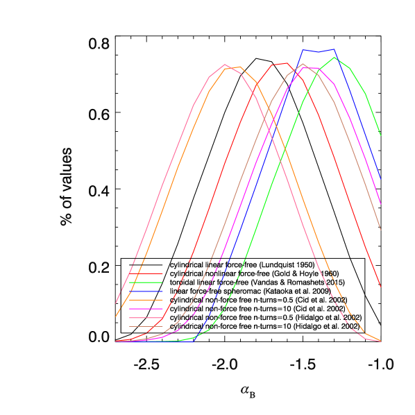
Figure 2.: Fraction of ${B_{\textrm{1 AU}}}$ values falling within the observed $B_{\textrm{MC}}$ range of 4 – 45 nT as a function of ${\alpha}_{B}$ for the various employed models.fig:fig2

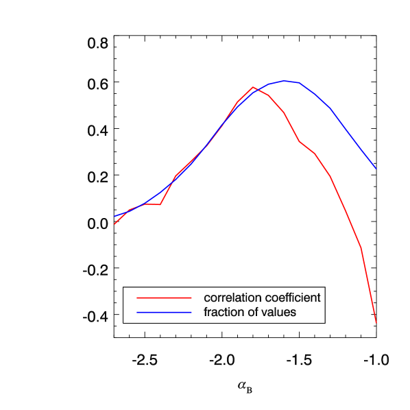
Figure 3.: Model-averaged correlation coefficient of the PDF for the predicted $B_{\textrm{1AU}}$ and observed $B_{\textrm{MC}}$ values at L1 as a function of ${\alpha}_{B}$ (red curve). Also shown is the respective fraction of ${B_{\textrm{1 AU}}}$ values (blue curve) falling within the observed $B_{\textrm{MC}}$ range. Both curves correspond to the respective averages of the various employed models as displayed in Figures fig:fig1 and fig:fig2.fig:fig3

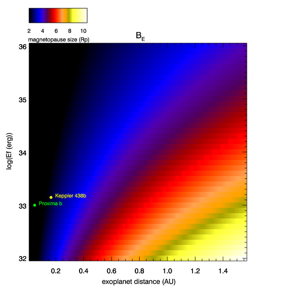
Figure 4.: Exoplanet magnetopause radius (in units of planet radius) required to counterbalance the magnetic pressure of a CME arriving at its vicinity as a function of the exoplanet distance to, and the associated flare energy of, the planet’s mother star. Magnetopause sizes smaller than 2, representing a lower limit of magnetospheric size to avoid atmospheric erosion, are saturated with black. The index ${\alpha}_{B}$ is assumed equal to be -1.6 and the Lundquist model is used. The yellow and green circles correspond to two case-studies of exoplanets Kepler 438b and Proxima b, orbiting stars exhibiting superflares. It is assumed that the exoplanets have an equatorial magnetic field equal to the terrestrial one, $B_{E}$ $\approx 0.333$ G.fig:fig4

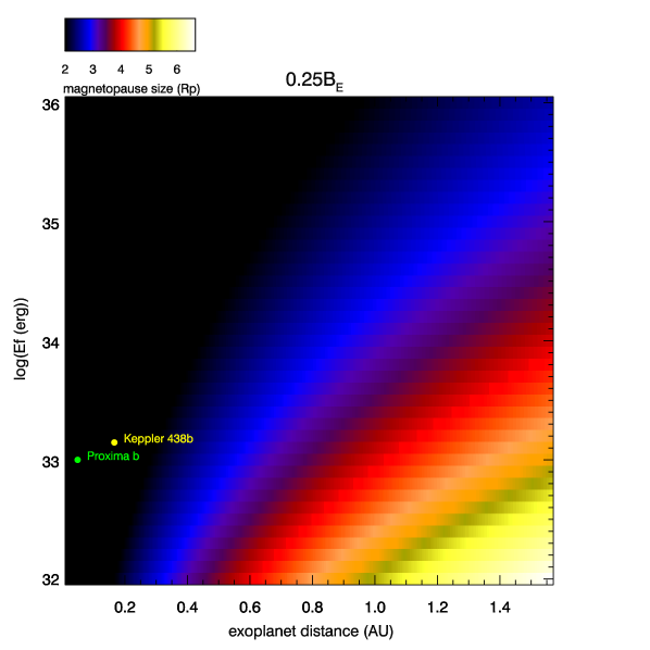
Figure 5.: Same as Figure fig:fig4, but for an exoplanet equatorial magnetic field of $\approx 0.083$ G, which is $\approx$ 25% of the terrestrial value.fig:fig5

Figure 6.: Same as Figure fig:fig4, but for an exoplanet equatorial magnetic field of $\approx 0.020$ G, $\approx$ 6.1% of the terrestrial value.fig:fig6

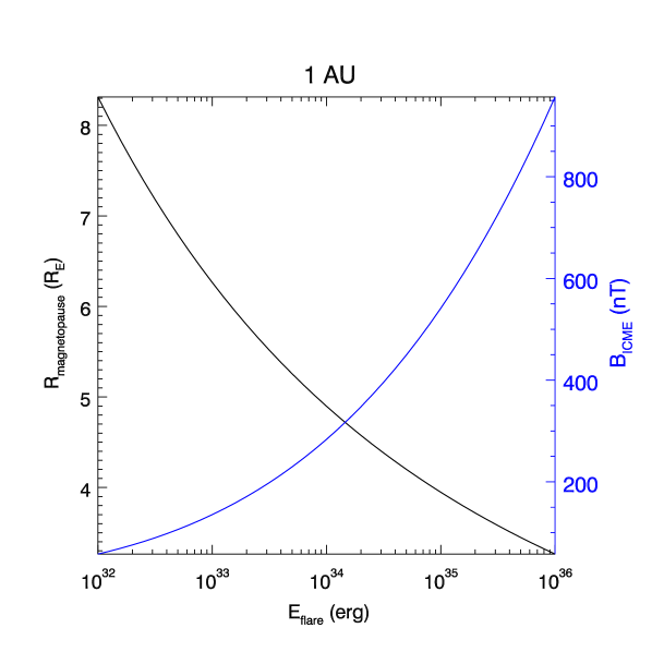
Figure 7.: Terrestrial magnetopause radius size (black) and ICME magnetic field magnitude at 1 AU (blue) as a function of flare energy. The index ${\alpha}_{B}$ is equal to -1.6 and the Lundquist model is used.fig:fig7

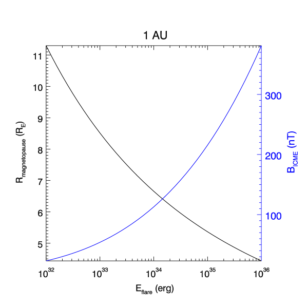
Figure 8.: Terrestrial magnetopause radius size (black) and ICME magnetic field magnitude at 1 AU (blue) as a function of flare energy. The index ${\alpha}_{B}$ is equal to -1.9 and the Lundquist model is used.fig:fig8

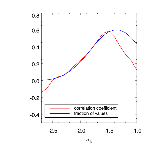
Figure 9.: Model-averaged correlation coefficient of the PDF for the predicted $B_{\textrm{1AU}}$ and observed $B_{\textrm{MC}}$ values at L1 as a function of ${\alpha}_{B}$ (red curve). Also shown is the respective fraction of ${B_{\textrm{1 AU}}}$ values (blue curve) falling within the observed $B_{\textrm{MC}}$ range. Calculations shown here are the same as in Figure fig:fig3 but use a randomly selected CME $H_{\textrm{m}}$ value in the range $10-40\%$ of the AR $H_{\textrm{m}}$ value (a fixed $100\%$ of the AR $H_{\textrm{m}}$ is used in Figure fig:fig3).fig:fig9

References

- Aarnio, Matt, and Stassun (2012) Aarnio, A.N., Matt, S.P., Stassun, K.G.: 2012, Mass Loss in Pre-main-sequence Stars via Coronal Mass Ejections and Implications for Angular Momentum Loss. ApJ 760, 9. DOI. ADS.
- Airapetian et al. (2017) Airapetian, V.S., Glocer, A., Khazanov, G.V., Loyd, R.O.P., France, K., Sojka, J., Danchi, W.C., Liemohn, M.W.: 2017, How Hospitable Are Space Weather Affected Habitable Zones? The Role of Ion Escape. ApJ 836, L3. DOI. ADS.
- Al-Haddad et al. (2013) Al-Haddad, N., Nieves-Chinchilla, T., Savani, N.P., Möstl, C., Marubashi, K., Hidalgo, M.A., Roussev, I.I., Poedts, S., Farrugia, C.J.: 2013, Magnetic Field Configuration Models and Reconstruction Methods for Interplanetary Coronal Mass Ejections. Sol. Phys. 284, 129. DOI. ADS.
- Andrews (2003) Andrews, M.D.: 2003, A Search for CMEs Associated with Big Flares. Sol. Phys. 218, 261. DOI. ADS.
- Anglada-Escudé et al. (2016) Anglada-Escudé, G., Amado, P.J., Barnes, J., Berdiñas, Z.M., Butler, R.P., Coleman, G.A.L., de La Cueva, I., Dreizler, S., Endl, M., Giesers, B., Jeffers, S.V., Jenkins, J.S., Jones, H.R.A., Kiraga, M., Kürster, M., López-González, M.J., Marvin, C.J., Morales, N., Morin, J., Nelson, R.P., Ortiz, J.L., Ofir, A., Paardekooper, S.-J., Reiners, A., Rodríguez, E., Rodríguez-López, C., Sarmiento, L.F., Strachan, J.P., Tsapras, Y., Tuomi, M., Zechmeister, M.: 2016, A terrestrial planet candidate in a temperate orbit around Proxima Centauri. Nature 536, 437. DOI. ADS.
- Armstrong et al. (2016) Armstrong, D.J., Pugh, C.E., Broomhall, A.-M., Brown, D.J.A., Lund, M.N., Osborn, H.P., Pollacco, D.L.: 2016, The host stars of Kepler’s habitable exoplanets: superflares, rotation and activity. MNRAS 455, 3110. DOI. ADS.
- Aulanier et al. (2013) Aulanier, G., Démoulin, P., Schrijver, C.J., Janvier, M., Pariat, E., Schmieder, B.: 2013, The standard flare model in three dimensions. II. Upper limit on solar flare energy. A&A 549, A66. DOI. ADS.
- Bastian et al. (2001) Bastian, T.S., Pick, M., Kerdraon, A., Maia, D., Vourlidas, A.: 2001, The Coronal Mass Ejection of 1998 April 20: Direct Imaging at Radio Wavelengths. ApJ 558, L65. DOI. ADS.
- Berger (1984) Berger, M.A.: 1984, Rigorous new limits on magnetic helicity dissipation in the solar corona. Geophys. Astrophys. Fluid Dyn. 30, 79. DOI. ADS.
- Bosman et al. (2012) Bosman, E., Bothmer, V., Nisticò, G., Vourlidas, A., Howard, R.A., Davies, J.A.: 2012, Three-Dimensional Properties of Coronal Mass Ejections from STEREO/SECCHI Observations. Sol. Phys. 281, 167. DOI. ADS.
- Bothmer and Schwenn (1998) Bothmer, V., Schwenn, R.: 1998, The structure and origin of magnetic clouds in the solar wind. Annales Geophysicae 16, 1. DOI. ADS.
- Chapman and Ferraro (1930) Chapman, S., Ferraro, V.C.A.: 1930, A New Theory of Magnetic Storms. Nature 126, 129. DOI. ADS.
- Chintzoglou, Patsourakos, and Vourlidas (2015) Chintzoglou, G., Patsourakos, S., Vourlidas, A.: 2015, Formation of Magnetic Flux Ropes during a Confined Flaring Well before the Onset of a Pair of Major Coronal Mass Ejections. ApJ 809, 34. DOI. ADS.
- Cid et al. (2002) Cid, C., Hidalgo, M.A., Nieves-Chinchilla, T., Sequeiros, J., Viñas, A.F.: 2002, Plasma and Magnetic Field Inside Magnetic Clouds: a Global Study. Sol. Phys. 207, 187. DOI. ADS.
- Cliver et al. (2014) Cliver, E.W., Tylka, A.J., Dietrich, W.F., Ling, A.G.: 2014, On a Solar Origin for the Cosmogenic Nuclide Event of 775 A.D. ApJ 781, 32. DOI. ADS.
- Cunha, Correia, and Laskar (2015) Cunha, D., Correia, A.C.M., Laskar, J.: 2015, Spin evolution of Earth-sized exoplanets, including atmospheric tides and core-mantle friction. International Journal of Astrobiology 14, 233. DOI. ADS.
- Dasso et al. (2006) Dasso, S., Mandrini, C.H., Démoulin, P., Luoni, M.L.: 2006, A new model-independent method to compute magnetic helicity in magnetic clouds. A&A 455, 349. DOI. ADS.
- Davenport et al. (2016) Davenport, J.R.A., Kipping, D.M., Sasselov, D., Matthews, J.M., Cameron, C.: 2016, MOST Observations of Our Nearest Neighbor: Flares on Proxima Centauri. ApJ 829, L31. DOI. ADS.
- Démoulin and Dasso (2009) Démoulin, P., Dasso, S.: 2009, Causes and consequences of magnetic cloud expansion. A&A 498, 551. DOI. ADS.
- Démoulin, Janvier, and Dasso (2016) Démoulin, P., Janvier, M., Dasso, S.: 2016, Magnetic Flux and Helicity of Magnetic Clouds. Sol. Phys. 291, 531. DOI. ADS.
- Démoulin et al. (2002) Démoulin, P., Mandrini, C.H., van Driel-Gesztelyi, L., Thompson, B.J., Plunkett, S., Kovári, Z., Aulanier, G., Young, A.: 2002, What is the source of the magnetic helicity shed by CMEs? The long-term helicity budget of AR 7978. A&A 382, 650. DOI. ADS.
- DeVore (2000) DeVore, C.R.: 2000, Magnetic Helicity Generation by Solar Differential Rotation. ApJ 539, 944. DOI. ADS.
- Donati et al. (2008) Donati, J.-F., Morin, J., Petit, P., Delfosse, X., Forveille, T., Aurière, M., Cabanac, R., Dintrans, B., Fares, R., Gastine, T., Jardine, M.M., Lignières, F., Paletou, F., Ramirez Velez, J.C., Théado, S.: 2008, Large-scale magnetic topologies of early M dwarfs. MNRAS 390, 545. DOI. ADS.
- Dong et al. (2017) Dong, C., Lingam, M., Ma, Y., Cohen, O.: 2017, Is Proxima Centauri b habitable? – A study of atmospheric loss. ArXiv e-prints. ADS.
- Drake et al. (2013) Drake, J.J., Cohen, O., Yashiro, S., Gopalswamy, N.: 2013, Implications of Mass and Energy Loss due to Coronal Mass Ejections on Magnetically Active Stars. ApJ 764, 170. DOI. ADS.
- Forbes (2000) Forbes, T.G.: 2000, A review on the genesis of coronal mass ejections. J. Geophys. Res. 105, 23153. DOI. ADS.
- Forsyth et al. (2006) Forsyth, R.J., Bothmer, V., Cid, C., Crooker, N.U., Horbury, T.S., Kecskemety, K., Klecker, B., Linker, J.A., Odstrcil, D., Reiner, M.J., Richardson, I.G., Rodriguez-Pacheco, J., Schmidt, J.M., Wimmer-Schweingruber, R.F.: 2006, ICMEs in the Inner Heliosphere: Origin, Evolution and Propagation Effects. Report of Working Group G. Space Sci. Rev. 123, 383. DOI. ADS.
- Garraffo, Drake, and Cohen (2016) Garraffo, C., Drake, J.J., Cohen, O.: 2016, The Space Weather of Proxima Centauri b. ApJ 833, L4. DOI. ADS.
- Gary and Moore (2004) Gary, G.A., Moore, R.L.: 2004, Eruption of a Multiple-Turn Helical Magnetic Flux Tube in a Large Flare: Evidence for External and Internal Reconnection That Fits the Breakout Model of Solar Magnetic Eruptions. ApJ 611, 545. DOI. ADS.
- Georgoulis, Tziotziou, and Raouafi (2012) Georgoulis, M.K., Tziotziou, K., Raouafi, N.-E.: 2012, Magnetic Energy and Helicity Budgets in the Active-region Solar Corona. II. Nonlinear Force-free Approximation. ApJ 759, 1. DOI. ADS.
- Georgoulis et al. (2009) Georgoulis, M.K., Rust, D.M., Pevtsov, A.A., Bernasconi, P.N., Kuzanyan, K.M.: 2009, Solar Magnetic Helicity Injected into the Heliosphere: Magnitude, Balance, and Periodicities Over Solar Cycle 23. ApJ 705, L48. DOI. ADS.
- Gibson and Fan (2008) Gibson, S.E., Fan, Y.: 2008, Partially ejected flux ropes: Implications for interplanetary coronal mass ejections. J. Geophys. Res. Space Phys. 113, A09103. DOI. ADS.
- Gladman et al. (1996) Gladman, B., Quinn, D.D., Nicholson, P., Rand, R.: 1996, Synchronous Locking of Tidally Evolving Satellites. Icarus 122, 166. DOI. ADS.
- Gold and Hoyle (1960) Gold, T., Hoyle, F.: 1960, On the origin of solar flares. MNRAS 120, 89. DOI. ADS.
- Good et al. (2015) Good, S.W., Forsyth, R.J., Raines, J.M., Gershman, D.J., Slavin, J.A., Zurbuchen, T.H.: 2015, Radial Evolution of a Magnetic Cloud: MESSENGER, STEREO, and Venus Express Observations. ApJ 807, 177. DOI. ADS.
- Green et al. (2002) Green, L.M., López fuentes, M.C., Mandrini, C.H., Démoulin, P., Van Driel-Gesztelyi, L., Culhane, J.L.: 2002, The Magnetic Helicity Budget of a cme-Prolific Active Region. Sol. Phys. 208, 43. DOI. ADS.
- Grießmeier et al. (2004) Grießmeier, J.-M., Stadelmann, A., Penz, T., Lammer, H., Selsis, F., Ribas, I., Guinan, E.F., Motschmann, U., Biernat, H.K., Weiss, W.W.: 2004, The effect of tidal locking on the magnetospheric and atmospheric evolution of “Hot Jupiters”. A&A 425, 753. DOI. ADS.
- Grießmeier et al. (2005) Grießmeier, J.-M., Stadelmann, A., Motschmann, U., Belisheva, N.K., Lammer, H., Biernat, H.K.: 2005, Cosmic Ray Impact on Extrasolar Earth-Like Planets in Close-in Habitable Zones. Astrobiology 5, 587. DOI. ADS.
- Guo et al. (2013) Guo, Y., Ding, M.D., Cheng, X., Zhao, J., Pariat, E.: 2013, Twist Accumulation and Topology Structure of a Solar Magnetic Flux Rope. ApJ 779, 157. DOI. ADS.
- Hariharan et al. (2016) Hariharan, K., Ramesh, R., Kathiravan, C., Wang, T.J.: 2016, Simultaneous Near-Sun Observations of a Moving Type IV Radio Burst and the Associated White-Light Coronal Mass Ejection. Sol. Phys. 291, 1405. DOI. ADS.
- Harra et al. (2016) Harra, L.K., Schrijver, C.J., Janvier, M., Toriumi, S., Hudson, H., Matthews, S., Woods, M.M., Hara, H., Guedel, M., Kowalski, A., Osten, R., Kusano, K., Lueftinger, T.: 2016, The Characteristics of Solar X-Class Flares and CMEs: A Paradigm for Stellar Superflares and Eruptions? Sol. Phys. 291, 1761. DOI. ADS.
- Hidalgo et al. (2000) Hidalgo, M.A., Cid, C., Medina, J., Viñas, A.F.: 2000, A new model for the topology of magnetic clouds in the solar wind. Sol. Phys. 194, 165. DOI. ADS.
- Houdebine, Foing, and Rodono (1990) Houdebine, E.R., Foing, B.H., Rodono, M.: 1990, Dynamics of flares on late-type dMe stars. I - Flare mass ejections and stellar evolution. A&A 238, 249. ADS.
- Howard et al. (2016) Howard, T.A., Stovall, K., Dowell, J., Taylor, G.B., White, S.M.: 2016, Measuring the Magnetic Field of Coronal Mass Ejections Near the Sun Using Pulsars. ApJ 831, 208. DOI. ADS.
- Hu et al. (2014) Hu, Q., Qiu, J., Dasgupta, B., Khare, A., Webb, G.M.: 2014, Structures of Interplanetary Magnetic Flux Ropes and Comparison with Their Solar Sources. ApJ 793, 53. DOI. ADS.
- Isavnin, Vourlidas, and Kilpua (2014) Isavnin, A., Vourlidas, A., Kilpua, E.K.J.: 2014, Three-Dimensional Evolution of Flux-Rope CMEs and Its Relation to the Local Orientation of the Heliospheric Current Sheet. Sol. Phys. 289, 2141. DOI. ADS.
- Jakosky et al. (2015) Jakosky, B.M., Grebowsky, J.M., Luhmann, J.G., Connerney, J., Eparvier, F., Ergun, R., Halekas, J., Larson, D., Mahaffy, P., McFadden, J., Mitchell, D.F., Schneider, N., Zurek, R., Bougher, S., Brain, D., Ma, Y.J., Mazelle, C., Andersson, L., Andrews, D., Baird, D., Baker, D., Bell, J.M., Benna, M., Chaffin, M., Chamberlin, P., Chaufray, Y.-Y., Clarke, J., Collinson, G., Combi, M., Crary, F., Cravens, T., Crismani, M., Curry, S., Curtis, D., Deighan, J., Delory, G., Dewey, R., DiBraccio, G., Dong, C., Dong, Y., Dunn, P., Elrod, M., England, S., Eriksson, A., Espley, J., Evans, S., Fang, X., Fillingim, M., Fortier, K., Fowler, C.M., Fox, J., Gröller, H., Guzewich, S., Hara, T., Harada, Y., Holsclaw, G., Jain, S.K., Jolitz, R., Leblanc, F., Lee, C.O., Lee, Y., Lefevre, F., Lillis, R., Livi, R., Lo, D., Mayyasi, M., McClintock, W., McEnulty, T., Modolo, R., Montmessin, F., Morooka, M., Nagy, A., Olsen, K., Peterson, W., Rahmati, A., Ruhunusiri, S., Russell, C.T., Sakai, S., Sauvaud, J.-A., Seki, K., Steckiewicz, M., Stevens, M., Stewart, A.I.F., Stiepen, A., Stone, S., Tenishev, V., Thiemann, E., Tolson, R., Toublanc, D., Vogt, M., Weber, T., Withers, P., Woods, T., Yelle, R.: 2015, MAVEN observations of the response of Mars to an interplanetary coronal mass ejection. Science 350, 0210. DOI. ADS.
- Jensen and Russell (2008) Jensen, E.A., Russell, C.T.: 2008, Faraday rotation observations of CMEs. Geophys. Res. Lett. 35, L02103. DOI. ADS.
- Kane et al. (2016) Kane, S.R., Hill, M.L., Kasting, J.F., Kopparapu, R.K., Quintana, E.V., Barclay, T., Batalha, N.M., Borucki, W.J., Ciardi, D.R., Haghighipour, N., Hinkel, N.R., Kaltenegger, L., Selsis, F., Torres, G.: 2016, A Catalog of Kepler Habitable Zone Exoplanet Candidates. ApJ 830, 1. DOI. ADS.
- Karoff et al. (2016) Karoff, C., Knudsen, M.F., De Cat, P., Bonanno, A., Fogtmann-Schulz, A., Fu, J., Frasca, A., Inceoglu, F., Olsen, J., Zhang, Y., Hou, Y., Wang, Y., Shi, J., Zhang, W.: 2016, Observational evidence for enhanced magnetic activity of superflare stars. Nature Communications 7, 11058. DOI. ADS.
- Kasting, Whitmire, and Reynolds (1993) Kasting, J.F., Whitmire, D.P., Reynolds, R.T.: 1993, Habitable Zones around Main Sequence Stars. Icarus 101, 108. DOI. ADS.
- Kataoka et al. (2009) Kataoka, R., Ebisuzaki, T., Kusano, K., Shiota, D., Inoue, S., Yamamoto, T.T., Tokumaru, M.: 2009, Three-dimensional MHD modeling of the solar wind structures associated with 13 December 2006 coronal mass ejection. J. Geophys. Res. Space Phys. 114, A10102. DOI. ADS.
- Kay, Opher, and Evans (2013) Kay, C., Opher, M., Evans, R.M.: 2013, Forecasting a Coronal Mass Ejection’s Altered Trajectory: ForeCAT. ApJ 775, 5. DOI. ADS.
- Kay, Opher, and Kornbleuth (2016) Kay, C., Opher, M., Kornbleuth, M.: 2016, Probability of CME Impact on Exoplanets Orbiting M Dwarfs and Solar-like Stars. ApJ 826, 195. DOI. ADS.
- Kazachenko et al. (2009) Kazachenko, M.D., Canfield, R.C., Longcope, D.W., Qiu, J., Des Jardins, A., Nightingale, R.W.: 2009, Sunspot Rotation, Flare Energetics, and Flux Rope Helicity: The Eruptive Flare on 2005 May 13. ApJ 704, 1146. DOI. ADS.
- Khodachenko et al. (2007) Khodachenko, M.L., Ribas, I., Lammer, H., Grießmeier, J.-M., Leitner, M., Selsis, F., Eiroa, C., Hanslmeier, A., Biernat, H.K., Farrugia, C.J., Rucker, H.O.: 2007, Coronal Mass Ejection (CME) Activity of Low Mass M Stars as An Important Factor for The Habitability of Terrestrial Exoplanets. I. CME Impact on Expected Magnetospheres of Earth-Like Exoplanets in Close-In Habitable Zones. Astrobiology 7, 167. DOI. ADS.
- Kliem, Rust, and Seehafer (2011) Kliem, B., Rust, S., Seehafer, N.: 2011, Helicity transport in a simulated coronal mass ejection. In: Bonanno, A., de Gouveia Dal Pino, E., Kosovichev, A.G. (eds.) Advances in Plasma Astrophysics, IAU Symposium 274, 125. DOI. ADS.
- Kooi et al. (2016) Kooi, J.E., Fischer, P.D., Buffo, J.J., Spangler, S.R.: 2016, VLA Measurements of Faraday Rotation through Coronal Mass Ejections. ArXiv e-prints. ADS.
- Kumar and Rust (1996) Kumar, A., Rust, D.M.: 1996, Interplanetary magnetic clouds, helicity conservation, and current-core flux-ropes. J. Geophys. Res. 101, 15667. DOI. ADS.
- Kunkel and Chen (2010) Kunkel, V., Chen, J.: 2010, Evolution of a Coronal Mass Ejection and its Magnetic Field in Interplanetary Space. ApJ 715, L80. DOI. ADS.
- Lammer et al. (2007) Lammer, H., Lichtenegger, H.I.M., Kulikov, Y.N., Grießmeier, J.-M., Terada, N., Erkaev, N.V., Biernat, H.K., Khodachenko, M.L., Ribas, I., Penz, T., Selsis, F.: 2007, Coronal Mass Ejection (CME) Activity of Low Mass M Stars as An Important Factor for The Habitability of Terrestrial Exoplanets. II. CME-Induced Ion Pick Up of Earth-like Exoplanets in Close-In Habitable Zones. Astrobiology 7, 185. DOI. ADS.
- Leconte et al. (2015) Leconte, J., Wu, H., Menou, K., Murray, N.: 2015, Asynchronous rotation of Earth-mass planets in the habitable zone of lower-mass stars. Science 347, 632. DOI. ADS.
- Leitner et al. (2007) Leitner, M., Farrugia, C.J., MöStl, C., Ogilvie, K.W., Galvin, A.B., Schwenn, R., Biernat, H.K.: 2007, Consequences of the force-free model of magnetic clouds for their heliospheric evolution. J. Geophys. Res. Space Phys. 112, A06113. DOI. ADS.
- Leitzinger et al. (2011) Leitzinger, M., Odert, P., Ribas, I., Hanslmeier, A., Lammer, H., Khodachenko, M.L., Zaqarashvili, T.V., Rucker, H.O.: 2011, Search for indications of stellar mass ejections using FUV spectra. A&A 536, A62. DOI. ADS.
- Leitzinger et al. (2014) Leitzinger, M., Odert, P., Greimel, R., Korhonen, H., Guenther, E.W., Hanslmeier, A., Lammer, H., Khodachenko, M.L.: 2014, A search for flares and mass ejections on young late-type stars in the open cluster Blanco-1. MNRAS 443, 898. DOI. ADS.
- Lepping et al. (2006) Lepping, R.P., Berdichevsky, D.B., Wu, C.-C., Szabo, A., Narock, T., Mariani, F., Lazarus, A.J., Quivers, A.J.: 2006, A summary of WIND magnetic clouds for years 1995-2003: model-fitted parameters, associated errors and classifications. Annales Geophysicae 24, 215. DOI. ADS.
- Liu, Richardson, and Belcher (2005) Liu, Y., Richardson, J.D., Belcher, J.W.: 2005, A statistical study of the properties of interplanetary coronal mass ejections from 0.3 to 5.4 AU. Planet. Space Sci. 53, 3. DOI. ADS.
- Lundquist (1950) Lundquist, S.: 1950,. Ark. Fys. 2(361).
- Luoni et al. (2005) Luoni, M.L., Mandrini, C.H., Dasso, S., van Driel-Gesztelyi, L., Démoulin, P.: 2005, Tracing magnetic helicity from the solar corona to the interplanetary space. Journal of Atmospheric and Solar-Terrestrial Physics 67, 1734. DOI. ADS.
- Lynch et al. (2003) Lynch, B.J., Zurbuchen, T.H., Fisk, L.A., Antiochos, S.K.: 2003, Internal structure of magnetic clouds: Plasma and composition. J. Geophys. Res. Space Phys. 108, 1239. DOI. ADS.
- Lynch et al. (2005) Lynch, B.J., Gruesbeck, J.R., Zurbuchen, T.H., Antiochos, S.K.: 2005, Solar cycle-dependent helicity transport by magnetic clouds. J. Geophys. Res. Space Phys. 110, A08107. DOI. ADS.
- Lynch et al. (2008) Lynch, B.J., Antiochos, S.K., DeVore, C.R., Luhmann, J.G., Zurbuchen, T.H.: 2008, Topological Evolution of a Fast Magnetic Breakout CME in Three Dimensions. ApJ 683, 1192. DOI. ADS.
- MacNeice et al. (2004) MacNeice, P., Antiochos, S.K., Phillips, A., Spicer, D.S., DeVore, C.R., Olson, K.: 2004, A Numerical Study of the Breakout Model for Coronal Mass Ejection Initiation. ApJ 614, 1028. DOI. ADS.
- Maehara et al. (2012) Maehara, H., Shibayama, T., Notsu, S., Notsu, Y., Nagao, T., Kusaba, S., Honda, S., Nogami, D., Shibata, K.: 2012, Superflares on solar-type stars. Nature 485, 478. DOI. ADS.
- Mancuso and Garzelli (2013) Mancuso, S., Garzelli, M.V.: 2013, Radial profile of the inner heliospheric magnetic field as deduced from Faraday rotation observations. A&A 553, A100. DOI. ADS.
- Mandrini et al. (2005) Mandrini, C.H., Pohjolainen, S., Dasso, S., Green, L.M., Démoulin, P., van Driel-Gesztelyi, L., Copperwheat, C., Foley, C.: 2005, Interplanetary flux rope ejected from an X-ray bright point. The smallest magnetic cloud source-region ever observed. A&A 434, 725. DOI. ADS.
- Moraitis et al. (2014) Moraitis, K., Tziotziou, K., Georgoulis, M.K., Archontis, V.: 2014, Validation and Benchmarking of a Practical Free Magnetic Energy and Relative Magnetic Helicity Budget Calculation in Solar Magnetic Structures. Sol. Phys. 289, 4453. DOI. ADS.
- Möstl et al. (2012) Möstl, C., Farrugia, C.J., Kilpua, E.K.J., Jian, L.K., Liu, Y., Eastwood, J.P., Harrison, R.A., Webb, D.F., Temmer, M., Odstrcil, D., Davies, J.A., Rollett, T., Luhmann, J.G., Nitta, N., Mulligan, T., Jensen, E.A., Forsyth, R., Lavraud, B., de Koning, C.A., Veronig, A.M., Galvin, A.B., Zhang, T.L., Anderson, B.J.: 2012, Multi-point Shock and Flux Rope Analysis of Multiple Interplanetary Coronal Mass Ejections around 2010 August 1 in the Inner Heliosphere. ApJ 758, 10. DOI. ADS.
- Nakwacki et al. (2011) Nakwacki, M.S., Dasso, S., Démoulin, P., Mandrini, C.H., Gulisano, A.M.: 2011, Dynamical evolution of a magnetic cloud from the Sun to 5.4 AU. A&A 535, A52. DOI. ADS.
- Nieves-Chinchilla et al. (2016) Nieves-Chinchilla, T., Linton, M.G., Hidalgo, M.A., Vourlidas, A., Savani, N.P., Szabo, A., Farrugia, C., Yu, W.: 2016, A Circular-cylindrical Flux-rope Analytical Model for Magnetic Clouds. ApJ 823, 27. DOI. ADS.
- Nindos and Andrews (2004) Nindos, A., Andrews, M.D.: 2004, The Association of Big Flares and Coronal Mass Ejections: What Is the Role of Magnetic Helicity? ApJ 616, L175. DOI. ADS.
- Nindos, Zhang, and Zhang (2003) Nindos, A., Zhang, J., Zhang, H.: 2003, The Magnetic Helicity Budget of Solar Active Regions and Coronal Mass Ejections. ApJ 594, 1033. DOI. ADS.
- Nindos et al. (2015) Nindos, A., Patsourakos, S., Vourlidas, A., Tagikas, C.: 2015, How Common Are Hot Magnetic Flux Ropes in the Low Solar Corona? A Statistical Study of EUV Observations. ApJ 808, 117. DOI. ADS.
- Nogami et al. (2014) Nogami, D., Notsu, Y., Honda, S., Maehara, H., Notsu, S., Shibayama, T., Shibata, K.: 2014, Two sun-like superflare stars rotating as slow as the Sun*. PASJ 66, L4. DOI. ADS.
- Osten and Wolk (2015) Osten, R.A., Wolk, S.J.: 2015, Connecting Flares and Transient Mass-loss Events in Magnetically Active Stars. ApJ 809, 79. DOI. ADS.
- Osten et al. (2013) Osten, R., Livio, M., Lubow, S., Pringle, J.E., Soderblom, D., Valenti, J.: 2013, Coronal Mass Ejections as a Mechanism for Producing IR Variability in Debris Disks. ApJ 765, L44. DOI. ADS.
- Pariat et al. (2006) Pariat, E., Nindos, A., Démoulin, P., Berger, M.A.: 2006, What is the spatial distribution of magnetic helicity injected in a solar active region? A&A 452, 623. DOI. ADS.
- Patsourakos and Georgoulis (2016) Patsourakos, S., Georgoulis, M.K.: 2016, Near-Sun and 1 AU magnetic field of coronal mass ejections: a parametric study. A&A 595, A121. DOI. ADS.
- Patsourakos et al. (2016) Patsourakos, S., Georgoulis, M.K., Vourlidas, A., Nindos, A., Sarris, T., Anagnostopoulos, G., Anastasiadis, A., Chintzoglou, G., Daglis, I.A., Gontikakis, C., Hatzigeorgiu, N., Iliopoulos, A.C., Katsavrias, C., Kouloumvakos, A., Moraitis, K., Nieves-Chinchilla, T., Pavlos, G., Sarafopoulos, D., Syntelis, P., Tsironis, C., Tziotziou, K., Vogiatzis, I.I., Balasis, G., Georgiou, M., Karakatsanis, L.P., Malandraki, O.E., Papadimitriou, C., Odstrčil, D., Pavlos, E.G., Podlachikova, O., Sandberg, I., Turner, D.L., Xenakis, M.N., Sarris, E., Tsinganos, K., Vlahos, L.: 2016, The Major Geoeffective Solar Eruptions of 2012 March 7: Comprehensive Sun-to-Earth Analysis. ApJ 817, 14. DOI. ADS.
- Patzold et al. (1987) Patzold, M., Bird, M.K., Volland, H., Levy, G.S., Seidel, B.L., Stelzried, C.T.: 1987, The mean coronal magnetic field determined from HELIOS Faraday rotation measurements. Sol. Phys. 109, 91. DOI. ADS.
- Poomvises et al. (2012) Poomvises, W., Gopalswamy, N., Yashiro, S., Kwon, R.-Y., Olmedo, O.: 2012, Determination of the Heliospheric Radial Magnetic Field from the Standoff Distance of a CME-driven Shock Observed by the STEREO Spacecraft. ApJ 758, 118. DOI. ADS.
- Priest, Longcope, and Janvier (2016) Priest, E.R., Longcope, D.W., Janvier, M.: 2016, Evolution of Magnetic Helicity During Eruptive Flares and Coronal Mass Ejections. Sol. Phys. 291, 2017. DOI. ADS.
- Régnier and Canfield (2006) Régnier, S., Canfield, R.C.: 2006, Evolution of magnetic fields and energetics of flares in active region 8210. A&A 451, 319. DOI. ADS.
- Riley et al. (2004) Riley, P., Linker, J.A., Lionello, R., Mikić, Z., Odstrcil, D., Hidalgo, M.A., Cid, C., Hu, Q., Lepping, R.P., Lynch, B.J., Rees, A.: 2004, Fitting flux ropes to a global MHD solution: a comparison of techniques. Journal of Atmospheric and Solar-Terrestrial Physics 66, 1321. DOI. ADS.
- Savani et al. (2015) Savani, N.P., Vourlidas, A., Szabo, A., Mays, M.L., Richardson, I.G., Thompson, B.J., Pulkkinen, A., Evans, R., Nieves-Chinchilla, T.: 2015, Predicting the magnetic vectors within coronal mass ejections arriving at Earth: 1. Initial architecture. Space Weather 13, 374. DOI. ADS.
- Scalo et al. (2007) Scalo, J., Kaltenegger, L., Segura, A.G., Fridlund, M., Ribas, I., Kulikov, Y.N., Grenfell, J.L., Rauer, H., Odert, P., Leitzinger, M., Selsis, F., Khodachenko, M.L., Eiroa, C., Kasting, J., Lammer, H.: 2007, M Stars as Targets for Terrestrial Exoplanet Searches And Biosignature Detection. Astrobiology 7, 85. DOI. ADS.
- Schrijver et al. (2012) Schrijver, C.J., Beer, J., Baltensperger, U., Cliver, E.W., Güdel, M., Hudson, H.S., McCracken, K.G., Osten, R.A., Peter, T., Soderblom, D.R., Usoskin, I.G., Wolff, E.W.: 2012, Estimating the frequency of extremely energetic solar events, based on solar, stellar, lunar, and terrestrial records. J. Geophys. Res. Space Phys. 117, A08103. DOI. ADS.
- See et al. (2014) See, V., Jardine, M., Vidotto, A.A., Petit, P., Marsden, S.C., Jeffers, S.V., do Nascimento, J.D.: 2014, The effects of stellar winds on the magnetospheres and potential habitability of exoplanets. A&A 570, A99. DOI. ADS.
- Selsis et al. (2007) Selsis, F., Kasting, J.F., Levrard, B., Paillet, J., Ribas, I., Delfosse, X.: 2007, Habitable planets around the star Gliese 581? A&A 476, 1373. DOI. ADS.
- Semel (1989) Semel, M.: 1989, Zeeman-Doppler imaging of active stars. I - Basic principles. A&A 225, 456. ADS.
- Shibata et al. (2013) Shibata, K., Isobe, H., Hillier, A., Choudhuri, A.R., Maehara, H., Ishii, T.T., Shibayama, T., Notsu, S., Notsu, Y., Nagao, T., Honda, S., Nogami, D.: 2013, Can Superflares Occur on Our Sun? PASJ 65, 49. DOI. ADS.
- Shibayama et al. (2013) Shibayama, T., Maehara, H., Notsu, S., Notsu, Y., Nagao, T., Honda, S., Ishii, T.T., Nogami, D., Shibata, K.: 2013, Superflares on Solar-type Stars Observed with Kepler. I. Statistical Properties of Superflares. ApJS 209, 5. DOI. ADS.
- Sun et al. (2012) Sun, X., Hoeksema, J.T., Liu, Y., Wiegelmann, T., Hayashi, K., Chen, Q., Thalmann, J.: 2012, Evolution of Magnetic Field and Energy in a Major Eruptive Active Region Based on SDO/HMI Observation. ApJ 748, 77. DOI. ADS.
- Thernisien, Vourlidas, and Howard (2009) Thernisien, A., Vourlidas, A., Howard, R.A.: 2009, Forward Modeling of Coronal Mass Ejections Using STEREO/SECCHI Data. Sol. Phys. 256, 111. DOI. ADS.
- Toriumi et al. (2017) Toriumi, S., Schrijver, C.J., Harra, L.K., Hudson, H., Nagashima, K.: 2017, Magnetic Properties of Solar Active Regions That Govern Large Solar Flares and Eruptions. ApJ 834, 56. DOI. ADS.
- Torres et al. (2015) Torres, G., Kipping, D.M., Fressin, F., Caldwell, D.A., Twicken, J.D., Ballard, S., Batalha, N.M., Bryson, S.T., Ciardi, D.R., Henze, C.E., Howell, S.B., Isaacson, H.T., Jenkins, J.M., Muirhead, P.S., Newton, E.R., Petigura, E.A., Barclay, T., Borucki, W.J., Crepp, J.R., Everett, M.E., Horch, E.P., Howard, A.W., Kolbl, R., Marcy, G.W., McCauliff, S., Quintana, E.V.: 2015, Validation of 12 Small Kepler Transiting Planets in the Habitable Zone. ApJ 800, 99. DOI. ADS.
- Tun and Vourlidas (2013) Tun, S.D., Vourlidas, A.: 2013, Derivation of the Magnetic Field in a Coronal Mass Ejection Core via Multi-frequency Radio Imaging. ApJ 766, 130. DOI. ADS.
- Tziotziou, Georgoulis, and Liu (2013) Tziotziou, K., Georgoulis, M.K., Liu, Y.: 2013, Interpreting Eruptive Behavior in NOAA AR 11158 via the Region’s Magnetic Energy and Relative-helicity Budgets. ApJ 772, 115. DOI. ADS.
- Tziotziou, Georgoulis, and Raouafi (2012) Tziotziou, K., Georgoulis, M.K., Raouafi, N.-E.: 2012, The Magnetic Energy-Helicity Diagram of Solar Active Regions. ApJ 759, L4. DOI. ADS.
- Usoskin et al. (2013) Usoskin, I.G., Kromer, B., Ludlow, F., Beer, J., Friedrich, M., Kovaltsov, G.A., Solanki, S.K., Wacker, L.: 2013, The AD775 cosmic event revisited: the Sun is to blame. A&A 552, L3. DOI. ADS.
- Valori, Démoulin, and Pariat (2012) Valori, G., Démoulin, P., Pariat, E.: 2012, Comparing Values of the Relative Magnetic Helicity in Finite Volumes. Sol. Phys. 278, 347. DOI. ADS.
- Vandas and Romashets (2016) Vandas, M., Romashets, E.: 2016, Toroidal linear force-free magnetic fields with axial symmetry. A&A 585, A108. DOI. ADS.
- Vidotto et al. (2013) Vidotto, A.A., Jardine, M., Morin, J., Donati, J.-F., Lang, P., Russell, A.J.B.: 2013, Effects of M dwarf magnetic fields on potentially habitable planets. A&A 557, A67. DOI. ADS.
- Vidotto et al. (2014) Vidotto, A.A., Gregory, S.G., Jardine, M., Donati, J.F., Petit, P., Morin, J., Folsom, C.P., Bouvier, J., Cameron, A.C., Hussain, G., Marsden, S., Waite, I.A., Fares, R., Jeffers, S., do Nascimento, J.D.: 2014, Stellar magnetism: empirical trends with age and rotation. MNRAS 441, 2361. DOI. ADS.
- Vourlidas et al. (2000) Vourlidas, A., Subramanian, P., Dere, K.P., Howard, R.A.: 2000, Large-Angle Spectrometric Coronagraph Measurements of the Energetics of Coronal Mass Ejections. ApJ 534, 456. DOI. ADS.
- Vrsnak et al. (1993) Vrsnak, B., Ruzdjak, V., Rompolt, B., Rosa, D., Zlobec, P.: 1993, Kinematics and evolution of twist in the eruptive prominence of August 18, 1980. Sol. Phys. 146, 147. DOI. ADS.
- Vršnak, Magdalenić, and Zlobec (2004) Vršnak, B., Magdalenić, J., Zlobec, P.: 2004, Band-splitting of coronal and interplanetary type II bursts. III. Physical conditions in the upper corona and interplanetary space. A&A 413, 753. DOI. ADS.
- Wang et al. (2016) Wang, Y., Zhuang, B., Hu, Q., Liu, R., Shen, C., Chi, Y.: 2016, On the twists of interplanetary magnetic flux ropes observed at 1 AU. J. Geophys. Res. Space Phys. 121, 9316. DOI. ADS.
- Winslow et al. (2015) Winslow, R.M., Lugaz, N., Philpott, L.C., Schwadron, N.A., Farrugia, C.J., Anderson, B.J., Smith, C.W.: 2015, Interplanetary coronal mass ejections from MESSENGER orbital observations at Mercury. J. Geophys. Res. Space Phys. 120, 6101. DOI. ADS.
- Wood, Howard, and Socker (2010) Wood, B.E., Howard, R.A., Socker, D.G.: 2010, Reconstructing the Morphology of an Evolving Coronal Mass Ejection. ApJ 715, 1524. DOI. ADS.
- Wu and Lepping (2005) Wu, C.-C., Lepping, R.P.: 2005, Relationships for predicting magnetic cloud-related geomagnetic storm intensity. Journal of Atmospheric and Solar-Terrestrial Physics 67, 283. DOI. ADS.
- Yashiro et al. (2005) Yashiro, S., Gopalswamy, N., Akiyama, S., Michalek, G., Howard, R.A.: 2005, Visibility of coronal mass ejections as a function of flare location and intensity. J. Geophys. Res. Space Phys. 110, A12S05. DOI. ADS.
- Zuluaga and Bustamante (2016) Zuluaga, J.I., Bustamante, S.: 2016, Geomagnetic properties of Proxima Centauri b analogues. ArXiv e-prints, Submitted to ApJL. ADS.