Crystalline evolutions with rapidly oscillating forcing terms

Abstract.

We consider the evolution by crystalline curvature of a planar set in a stratified medium, modeled by a periodic forcing term. We characterize the limit evolution law as the period of the oscillations tends to zero. Even if the model is very simple, the limit evolution problem is quite rich, and we discuss some properties such as uniqueness, comparison principle and pinning/depinning phenomena.

1. Introduction

In this paper we are interested in the asymptotic behaviour of motions of planar curves according to the law

(1) $$v=\kappa_{\varphi}+g\left(\frac{x}{\varepsilon}\right),$$

where $v$ is the normal velocity, $\kappa_{\varphi}$ is the crystalline square curvature (see Definition 2.1 for precise definitions), $g:\mathbb{R}\to\mathbb{R}$ is a forcing term depending only on the horizontal variable $x$, and $\varepsilon>0$ is a small parameter modeling the rapidly oscillating medium where the curve evolves. For simplicity, we shall assume that $g$ is 1-periodic and takes only two values $\alpha<0<\beta$, with average $\frac{\alpha+\beta}{2}$.

Crystalline evolutions play an important role in many models of phase transitions and Materials Science (see [28, 32] and references therein) and have been significantly studied in recent years (see for instance [1, 25, 6, 7, 23]). The term $g\left(\frac{x}{\varepsilon}\right)$ models a heterogeneous layered medium, which we assume periodic exactly in one of the direction orthogonal to the Wulff shape of the crystalline perimeter (in our case, for simplicity, the $x$-direction). Our aim is understanding the effect of the oscillations in the asymptotic limit $\varepsilon\to 0$, which is a typical homogenization problem.

We will show that, at scale $\varepsilon$, the curves may undergo a microscopic ‘facet breaking’ phenomenon, with small segments of length proportional to $\varepsilon$ being created and reabsorbed. After dealing with this aspect, we show that the motion of a limit of curves satisfying (1) can be characterized by different laws of motion in the $x$ and $y$ directions: the portions of the curve moving in the vertical direction travel with a velocity equal to $\kappa_{\varphi}+\frac{\alpha+\beta}{2}$, whereas the portions moving in the horizontal direction are either pinned or travel with velocity equal to $\langle\kappa_{\varphi}+g\rangle$, where $\langle\cdot\rangle$ denotes the harmonic mean (see Theorem 4.7). Note that such law does not correspond to a forced crystalline evolution.

Our analysis can be set in a large class of variational evolution problems dealing with limits of motions driven by functionals $F_{\varepsilon}$ depending on a small parameter [10]. In some cases, the limit motion can be directly related to the $\Gamma$-limit of $F_{\varepsilon}$ (see, e.g., [31, 20, 12, 14]), but in general this is not the case. For oscillating functionals, the energy landscape of the energies $F_{\varepsilon}$ can be quite different from that of their $\Gamma$-limit and the related motions can be influenced by the presence of local minima which may give rise to ‘pinning’ phenomena (motions may be attracted by those local minima) or to effective homogenized velocities [30, 13]. In the case of geometric motions, a general understanding of the effects of microstructure is still missing. Recently, some results have been obtained for (two-dimensional) crystalline energies, for which a simpler description can be sometimes given in terms of a system of ODEs. Such results include discrete approximations of crystalline energies, which can be understood as a simple way to introduce a periodic dependence, corresponding to that of an underlying square lattice [13, 15, 11, 16]. Such discrete energies correspond to continuum inhomogeneous perimeter energies of the form

$$F_{\varepsilon}(E)=\int_{\partial E}a\Bigl{(}\frac{x}{\varepsilon},\frac{y}{\varepsilon}\Bigr{)}\bigl{(}|\nu_{1}^{E}|+|\nu_{2}^{E}|\bigr{)}\,d\mathcal{H}^{1},\qquad E\subset\mathbb{R}^{2},$$

converging to the square perimeter in the sense of $\Gamma$-convergence [9, 3], and the corresponding geometric motions can be studied using the minimizing-movement approach introduced by Almgren, Taylor and Wang [2]. The suitably defined limit motions [10] correspond to modified crystalline flows.

In our case, equation (1) corresponds to the $L^{2}$-gradient flow for the energy functional

$$F_{\varepsilon}(E)=\int_{\partial E}\bigl{(}|\nu_{1}^{E}|+|\nu_{2}^{E}|\bigr{)}\,d\mathcal{H}^{1}+\int_{E}g\Bigl{(}\frac{x}{\varepsilon}\Bigr{)}\ d\mathcal{L}^{2},\qquad E\subset\mathbb{R}^{2},$$

where we identify the evolving curve with the boundary of a set $E$. Notice that, since the volume term converges to $\frac{\alpha+\beta}{2}\mathcal{L}^{2}(E)$, the ($\Gamma$-)limit as $\varepsilon\to 0$ of the functionals $F_{\varepsilon}$ is the functional

$$\overline{F}(E)=\int_{\partial E}\bigl{(}|\nu_{1}^{E}|+|\nu_{2}^{E}|\bigr{)}\,d\mathcal{H}^{1}+\dfrac{\alpha+\beta}{2}\mathcal{L}^{2}(E).$$

As a consequence of our analysis, it turns out that the asymptotic behavior as $\varepsilon\to 0$ of the evolutions corresponding to (1) does not coincide with the gradient flow of $\overline{F}$, which is $v=\kappa_{\varphi}+\frac{\alpha+\beta}{2}$. Even in the case $\alpha+\beta=0$ the limit motion cannot be derived as a gradient flow of a modified (crystalline) perimeter.

Note that, if the crystalline curvature is replaced by the usual curvature and the evolving curve is a unbounded graph in the vertical direction, so that it never travels horizontally, the analogous homogenization problem have been studied in [18], where it is proved that the limit evolution law is indeed the curvature flow with a constant forcing term. However, if the curve is a graph in the horizontal direction the problem is more complicated and a general convergence result is still not available. In this respect, our work is a step in that direction. We mention, however, that a complete analysis of the asymptotic behavior of the semlinear problem

$$u_{t}=u_{xx}+g\left(\frac{u}{\varepsilon}\right),$$

can be found in [17]. That problem has some features in common with our geometric evolution, as can be seen as the linearization of the isotropic version of (1).

The plan of the paper is the following: in Section 2 we introduce the notion of crystalline curvature and the evolution problem we want to study. In Section 3 we introduce the notion of calibrable edge, that is, an edge of the curve which does not break during the evolution, and we characterize the calibrability of an edge in terms of its length and of the position of its endpoints. Finally, in Section 4 we characterize the limit evolution law as $\varepsilon\to 0$ first for rectangular sets, then for polyrectangles, and eventually for more general sets, including bounded convex sets.

2. Setting of the problem

2.1. Notation

Given $\xi$ $\eta\in\mathbb{R}^{2}$, we denote by $\xi\cdot\eta$ the usual scalar product between $\xi$ and $\eta$ and by ${]\!]\xi,\eta[\![}$ (respectively, ${[\![\xi,\eta]\!]}$) the open (respectively, closed) segment joining $\xi$ with $\eta$. The canonical basis of $\mathbb{R}^{2}$ will be denoted by $e_{1}=(1,0)$, $e_{2}=(0,1)$.

The 1–dimensional Hausdorff measure and the 2–dimensional Lebesgue measure in $\mathbb{R}^{2}$ will be denoted by $\mathcal{H}^{1}$ and $\mathcal{L}^{2}$, respectively.

We say that a set $E\subseteq\mathbb{R}^{2}$ is a Lipschitz set if $E$ is open and $\partial E$ can be written, locally, as the graph of a Lipschitz function (with respect to a suitable orthogonal coordinate system). The outward normal to $\partial E$ at $\xi$, that exists $\mathcal{H}^{1}$–almost everywhere on $\partial E$, will be denoted by $\nu^{E}(\xi)=(\nu_{1}^{E},\nu_{2}^{E})$.

The Hausdorff distance between the two sets $E,\ F\in\mathbb{R}^{2}$ will be denoted by $d_{H}(E,F)$.

2.2. The crystalline square curvature

We briefly recall how to give a notion of mean curvature $\kappa^{E}$ which is consistent with the requirement that a geometric evolution $E(t)$ that reduces as fast as possible the energy functional

$$P(E)=\int_{\partial E}\bigl{(}|\nu_{1}^{E}|+|\nu_{2}^{E}|\bigr{)}\,d\mathcal{H}^{1}$$

has normal velocity $\kappa^{E(t)}$ $\mathcal{H}^{1}$–almost everywhere on $\partial E(t)$.

The functional $P(E)$ turns out to be the perimeter associated to the norm $\varphi(x,y)=\max\{|x|,|y|\}$, $(x,y)\in\mathbb{R}^{2}$, that is the Minkowski content derived by considering $(\mathbb{R}^{2},\varphi)$ as a normed space. The density $\varphi^{\circ}(x,y)=|x|+|y|$ is the polar function of $\varphi$, defined by $\varphi^{\circ}(\xi^{\circ}):=\sup\{\xi\cdot\xi^{\circ},\ \varphi(\xi)\leq 1\}$.

The sublevel sets (or Wulff shapes) $\{\phi(\xi)\leq 1\}$ and $\{\phi^{\circ}(\xi)\leq 1\}$ are the square $K=[-1,1]^{2}$, and the square with corners at $(\pm 1,0)$ and $(0,\pm 1)$, respectively.

Given a nonempty compact set $E\subseteq\mathbb{R}^{2}$, we denote by $d_{\varphi}^{E}$ the oriented $\varphi$–distance function to $\partial E$, negative inside $E$, that is

$$d_{\varphi}^{E}(\xi)=\inf_{\eta\in E}\varphi(\xi-\eta)-\inf_{\eta\not\in E}\varphi(\xi-\eta),\qquad\xi\in\mathbb{R}^{2}.$$

The function $d_{\varphi}^{E}$ is Lipschitz, $\varphi^{\circ}(\nabla d_{\varphi}^{E}(\xi))=1$ at each its differentiability point $\xi$, and

$$\nabla d_{\varphi}^{E}(\xi)=\frac{\nu_{E}(\xi)}{\varphi^{\circ}(\nu_{E}(\xi))}$$

at every $\xi\in\partial E$ where $\nu_{E}$ is well defined.

Due to the lack of uniqueness of the projection on $\partial E$ with respect to the distance $d_{\varphi}^{E}$, the intrinsic normal direction is not uniquely determined, in general, even if the set $E$ is smooth. It is known that the normal cone at $\xi\in\partial E$ is well defined whenever $\xi$ is a differentiability point for $d_{\varphi}^{E}$ and it is given by $T_{\phi^{\circ}}\bigl{(}\nabla d_{\varphi}^{E}(\xi)\bigr{)}$, where

$$T_{\varphi^{\circ}}(\xi^{\circ}):=\{\xi\in\mathbb{R}^{2},\xi\cdot\xi^{\circ}=(\varphi^{\circ}(\xi))^{2}\},\quad\xi^{\circ}\in\mathbb{R}^{2}\,.$$

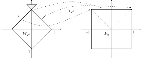
Figure 1. The square crystalline norm $\varphi$ and the map $T_{\varphi^{\circ}}$

If $\varphi^{\circ}(\xi^{\circ})=1$, a direct computation gives

(2) $$T_{\varphi^{\circ}}(\xi^{\circ})=\begin{cases}(1,1)&\xi^{\circ}\in{]\!]e_{1},e_{2}[\![}\\ (1,-1)&\xi^{\circ}\in{]\!]e_{1},-e_{2}[\![}\\ (-1,-1)&\xi^{\circ}\in{]\!]e_{2},-e_{1}[\![}\\ (-1,1)&\xi^{\circ}\in{]\!]-e_{2},-e_{1}[\![}\end{cases}\qquad\begin{cases}T_{\varphi^{\circ}}(e_{1})&={[\![(1,1),(1,-1)]\!]},\\ T_{\varphi^{\circ}}(e_{2})&={[\![(-1,1),(1,1)]\!]},\\ T_{\varphi^{\circ}}(-e_{1})&={[\![(-1,1),(-1,-1)]\!]},\\ T_{\varphi^{\circ}}(-e_{2})&={[\![(-1,-1),(1,-1)]\!]}.\end{cases}$$

(see Figure 1).

The notion of intrinsic curvature in $(\mathbb{R}^{2},\varphi)$ is based on the existence of regular selections of $T_{\phi^{\circ}}\bigl{(}\nabla d_{\varphi}^{E}\bigr{)}$ on $\partial E$.

Definition 2.1 ($\varphi$–regular set, Cahn–Hoffmann field, mean $\varphi$–curvature).

We say that an open set $E\subseteq\mathbb{R}^{2}$ is $\varphi$–regular if $\partial E$ is a compact Lipschitz curve, and there exists a vector field $n_{\varphi}\in\textrm{Lip}(\partial E;\mathbb{R}^{2})$ such that $n_{\varphi}\in T_{\varphi^{\circ}}(\nabla d_{\varphi}^{E})$ $\mathcal{H}^{1}$–almost everywhere in $\partial E$.

Any such a selection of the multivalued function $T_{\varphi^{\circ}}(\nabla d_{\varphi}^{E})$ on $\partial E$ is called a Cahn–Hoffmann vector field for $\partial E$ associated to $\varphi$, and $\kappa_{\varphi}=\operatorname{div}n_{\varphi}$ is the related mean $\varphi$–curvature (crystalline square mean curvature) of $\partial E$.

Remark 2.2.

Notice that, unlike the outer (euclidean) unit normal $\nu^{E}$, a Cahn–Hoffmann field is defined everywhere on $\partial E$.

Remark 2.3.

Any Cahn–Hoffmann vector field $n_{\varphi}$ has gradient orthogonal to the normal direction, so that $\operatorname{div}n_{\varphi}$ equals the tangential divergence of the field.

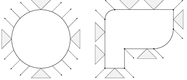
Figure 2. A non $\varphi$–regular set (left) and a $\varphi$–regular set (right)

Remark 2.4 (Edges and vertices).

The boundary of a $\varphi$–regular set $E$ is given by a finite number of closed arcs with the property that $T_{\varphi^{\circ}}(\nabla d_{\varphi}^{E})$ is a fixed set $T_{A}$ in the interior of each arc $A$ (see Figure 2). This set $T_{A}$ is either a singleton, if the arc $A$ is not a horizontal or vertical segment, or one of the closed convex cones described in (2). The arcs of $\partial E$ which are straight horizontal or vertical segments will be called edges, and the endpoints of every arc will be called vertices of $\partial E$.

Remark 2.5.

The requirement of Lipschitz continuity keeps the value of every Cahn–Hoffmann vector field fixed at vertices. Hence, in order to exhibit a Cahn–Hoffmann vector field $n_{\varphi}$ on $\partial E$ it is enough to construct a field $n_{A}\in\textrm{Lip}(A;\mathbb{R}^{2})$ on each arc $A$, with the correct values at the vertices, and satisfying the constraint $n_{A}\in T_{A}$. In what follows, with a little abuse of notation, we shall call $n_{A}$ the Cahn–Hoffmann vector field on the arc $A$.

2.3. Forced crystalline curvature flow

The appropriate way for describing a geometric evolution $E(t)$, starting from a given $\varphi$–regular set $E$, and trying to reduce as fast as possible the energy functional

$$F(E(t))=P_{\varphi}(E(t))+V(E(t))=\int_{\partial E(t)}\bigl{(}|\nu_{1}^{E}(t)|+|\nu_{2}^{E}(t)|\bigr{)}\,d\mathcal{H}^{1}+\int_{E(t)}f\ d\mathcal{L}^{2},$$

is a suitable weak version of the law

$$v=\kappa_{\varphi}+f,\qquad\text{on}\ E(t)$$

where $v$ is the scalar velocity of $\partial E(t)$ along the normal direction.

Definition 2.6.

Given $T>0$, we say that a family $E(t)$, $t\in[0,T]$, is a crystalline mean curvature flow in $[0,T)$ with forcing term $f\in L^{\infty}(\mathbb{R}^{2})$ if

• $E(t)\subseteq\mathbb{R}^{2}$ is a Lipschitz set for every $t\in[0,T)$;

• there exists an open set $A\subseteq\mathbb{R}^{2}\times[0,T)$ such that $\bigcup_{t\in[0,T)}\partial E(t)\times\{t\}\subseteq A$, and the function $d(\xi,t)\doteq d^{E(t)}_{\varphi}(\xi)$ is locally Lipschitz in $A$;

• there exists a function $n\in L^{\infty}(A,\mathbb{R}^{2})$, with $\operatorname{div}n\in L^{\infty}(A)$, such that the restriction of $n(t,\cdot)$ to $\partial E(t)$ is a Cahn–Hoffmann vector field for $\partial E(t)$ for every $t\in[0,T]$;

• $\partial_{t}d-\operatorname{div}n\in[f^{-},f^{+}]$ $\mathcal{H}^{1}$–almost everywhere in $\partial E(t)$ and for all $t\in[0,T)$, where

  $$f^{+}(\xi)=\text{ess}\limsup_{\eta\to\xi}f(\eta),\qquad f^{-}(\xi)=\text{ess}\liminf_{\eta\to\xi}f(\eta),\qquad\xi\in\mathbb{R}^{2}.$$

As underlined in Remark 2.5, the Cahn–Hoffmann vector field $n(t)$ on $\partial E(t)$ is obtained by gluing suitable fields constructed on each arc of the boundary. If an arc $A\subseteq\partial E(t)$ is not a edge, the Cahn–Hoffmann vector field $n(t)$ is uniquely determined by the geometry of $A$, and the $\varphi$–mean curvatures of at each point of $A$ is zero. On the other hand, there are infinitely many choices for the vector field in the interior of the edges on $\partial E(t)$, and hence infinitely many different $\varphi$–mean curvatures associated. Most of these choices are meaningless for the point of view of the geometric evolution. In order to overcome this ambiguity we fix the choice by a variational selection principle which turns out to be consistent with the curve shortening flow (see [6], [7], [8], [26], [27]).

Definition 2.7 (Variational forced crystalline curvature flow).

A variational forced crystalline curvature flow is a forced crystalline curvature flow $E(t)$, $t\in[0,T)$, such that for every $t\in[0,T)$ and for every edge $L$ of $\partial E(t)$ the Cahn–Hoffmann vector field $n_{L}$ is the unique minimum of the functional

$$\mathcal{N}_{L}(n)=\int_{L}|f-\operatorname{div}n|^{2}\,d\mathcal{H}^{1}$$

in the set

$$D_{L}=\left\{n\in L^{\infty}(L,\mathbb{R}^{2}),n\in T_{L},\operatorname{div}n\in L^{\infty}(L),n(p)=n_{0},n(q)=n_{1}\right\}$$

where $p$, $q$ are the endpoints of $L$ and $n_{0}$, $n_{1}$ are the values at the vertices $p$, $q$ assigned to every Cahn–Hoffmann vector field (see Remark 2.5).

Remark 2.8.

If the minimum $n_{L}$ in $D_{L}$ of the functional $\mathcal{N}_{L}$ satisfies the strict constraint $n_{L}(\xi)\in\operatorname{int}T_{L}$ for every $\xi\in L$, then the velocity $f-\operatorname{div}n_{L}$ is constant along the edge, that is the flat arc remains flat under the evolution. This is always the case when $f=0$, since the unique minimum is the interpolation of the assigned values at the vertices of $L$, and the constant value of the mean $\varphi$–curvature is given by

(3) $$\kappa_{\varphi}^{L}=\chi_{L}\frac{2}{\ell}\ \text{on}\ L,$$

where $\ell$ is the length of the edge $L$ and $\chi_{L}$ is a convexity factor: $\chi_{L}=1,-1,0$, depending on whether $E(t)$ is locally convex at $L$, locally concave at $L$, or neither.

We refer to [19, 24, 5] for some existence and uniqueness results for variational forced crystalline curvature flow, when the forcing term $f$ is a Lipschitz function. To the best of our knowledge, there is no general results for discontinuous forcing terms.

The easiest example of variational forced crystalline curvature flow is the one starting from a coordinate rectangle $R$ (rectangle with edges parallel to the coordinate axes), and with constant forcing term $f(\xi)=\gamma\in\mathbb{R}$.

Ordering the vertices of $\partial E$ clockwise starting from the left–upper corner, $P_{i}$, $i=1,\dots,4$, we have

$$n_{\varphi}(P_{1})=(-1,1),\quad n_{\varphi}(P_{2})=(1,1),\quad n_{\varphi}(P_{3})=(1,-1),\quad n_{\varphi}(P_{4})=(-1,-1),$$

and hence the variational Cahn–Hoffmann vector field on the sides is

$$n_{\varphi}(\xi)=n_{\varphi}(P_{i})+\frac{2(-1)^{i+1}}{\ell_{i}}(\xi-P_{i}),\qquad\xi\in L_{i},\ i=1,\dots,4,$$

where $L_{i}$ is the edge of the rectangle starting from $P_{i}$, and $\ell_{i}$ is its length.

The $\varphi$–curvature associated to this field is constant on each edge $L_{i}$, and

$$\kappa_{\varphi}^{i}=\frac{2(-1)^{i+1}}{\ell_{i}}\ \text{on}\ L_{i},\ i=1,\dots,4.$$

As a consequence the evolution of $R$ is given by rectangles $R(t)$, and the description of the flow reduces to the analysis of a system of ODE’s solved by the length $\ell_{1}(t)$ and $\ell_{2}(t)$ of the horizontal and the vertical edges of $R(t)$:

(4) $$\begin{cases}\ell_{1}^{\prime}=-\dfrac{4}{l_{2}}-2\gamma\,,\\[8.0pt] \ell_{2}^{\prime}=-\dfrac{4}{l_{1}}-2\gamma\,.\end{cases}$$

(see [1] and [25]). Hence, if $\gamma>0$, $\ell_{1}$ and $\ell_{2}$ are decreasing and we have finite–time extinction (see the phase portrait in the left–hand side of Figure 3), while if $\gamma<0$ the evolution is the one depicted in the right–hand side of Figure 3. The square of side length $\ell^{0}=-2/\gamma$ is the unique equilibrium of the system. Moreover, the function

$$U(\ell_{1},\ell_{2})=4(\log(\ell_{2})-\log(\ell_{1}))+2\gamma(\ell_{2}-\ell_{1})$$

is a constant of motion for the system (4). The squares starting with a side length shorter than $l^{0}$ shrink to a point, while the squares starting with a side length longer than $l^{0}$ expand with asymptotic velocity $-\gamma$ on each side as the side length diverges. The rectangles can shrink to a point, converge to the equilibrium or expand, depending on the starting length of the edges.

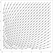
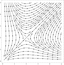
Figure 3. Phase portraits of (4) for $\gamma>0$ and for $\gamma<0$.

In general, in presence of a spatially inhomogeneous forcing term, the selfsimilarity of the evolution of coordinate rectangles may fail, due to the possibility of edge breaking/bending phenomena (see [26], [27]).

2.4. The oscillating forcing term

In what follows we will consider a prototypical case of oscillating layered forcing term: given two constants $\alpha<0<\beta$, let

(5) $$g(x)=\begin{cases}\alpha,&\text{if}\ \text{dist}(x,\mathbb{Z})\leq\dfrac{1}{4},\\ \beta,&\text{otherwise},\end{cases}$$

and let us denote by $\mathcal{I}$ the set of discontinuity lines of the function $g$:

$$\mathcal{I}:=\left\{(x,y),\ x\in\dfrac{1}{4}+\dfrac{1}{2}\mathbb{Z},\ y\in\mathbb{R}\right\}.$$

In order to distinguish the two families of discontinuity lines for $g$, depending on the position of the phases $\alpha$ and $\beta$ with respect to the interface, we will use the notation

$$\begin{split}\mathcal{I}_{\alpha,\beta}&:=\left\{(x,y),\ y\in\mathbb{R},\ x\in\mathbb{R}\ \text{such that}\ g(s,y)=\beta\ \forall s\in(x,x+1/2)\right\}\\ \mathcal{I}_{\beta,\alpha}&:=\left\{(x,y),\ y\in\mathbb{R},\ x\in\mathbb{R}\ \text{such that}\ g(s,y)=\alpha\ \forall s\in(x,x+1/2)\right\}.\end{split}$$

Given $\varepsilon>0$ we consider the function $g_{\varepsilon}$ defined by

$$g_{\varepsilon}(x,y):=g\left(\frac{x}{\varepsilon}\right).$$

(with an abuse of notation, we will often write $g_{\varepsilon}(x)$ instead of $g_{\varepsilon}(x,y)$). Setting

(6) $$x_{N}:=\left(N+\frac{1}{4}\right)\varepsilon,\qquad N\in\mathbb{N},$$

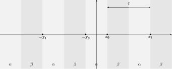
Figure 4. The oscillating forcing term $g_{\varepsilon}$

we have that

(7) $$g_{\varepsilon}(x,y)=\begin{cases}\alpha,&x\in\left(x_{N}-\dfrac{\varepsilon}{2},x_{N}\right),\ y\in\mathbb{R},\\[10.0pt] \beta,&x\in\left(x_{N},x_{N}+\dfrac{\varepsilon}{2}\right),\ y\in\mathbb{R},\end{cases}$$

that is $\{x=x_{N}\}\subseteq\varepsilon\mathcal{I}_{\alpha,\beta}$ and $\{x=-x_{N}\}\subseteq\varepsilon\mathcal{I}_{\beta,\alpha}$ for every $N\in\mathbb{N}$ (see Figure 4).

Finally, we define the multifunction

$$G_{\varepsilon}(x,y)=\begin{cases}g_{\varepsilon}(x,y),&\text{if}\ (x,y)\not\in\varepsilon\mathcal{I},\\ [\alpha,\beta],&\text{if}\ (x,y)\in\varepsilon\mathcal{I},\end{cases}$$

in such a way a variational crystalline mean curvature flow $E(t)$ with forcing term $g_{\varepsilon}$ has to have normal velocity $v(t)\in\operatorname{div}n(t)+G_{\varepsilon}$ on $\partial E(t)$.

3. Calibrable edges

In this section we keep $\varepsilon>0$ fixed, and we focus our attention on the effect of the forcing term $g_{\varepsilon}$ along a horizontal or vertical edge $L$.

Definition 3.1.

An edge $L$ of a $\varphi$–regular set $E$ is calibrable if there exists a Cahn–Hoffmann vector field $n$ for $\partial E$, and a constant $v\in\mathbb{R}$ such that $v\in\operatorname{div}n+G_{\varepsilon}$ on $L$. In this case we say that $v$ is a (normal) velocity of the edge $L$.

Remark 3.2.

In view of Remark 2.5, in order to show that an edge $L$ of $\partial E$ is calibrable it is enough to show that there exists a vector field $n$ on $L$, such that $n(\xi)\in T_{L}$ for every $\xi\in\operatorname{int}L$ and agrees with assigned values (prescribed by the geometry of $\partial E$) at the endpoints of $L$, .

In what follows, the length of an edge $L$ will be denoted by $\ell$.

3.1. Vertical edges

Every vertical edge is calibrable. Namely, if $x=\overline{x}\in\mathbb{R}$ is the straight line containing $L$, there exists a constant selection $\gamma_{\varepsilon}(\overline{x})$ of $G_{\varepsilon}$ on $L$, and hence the Cahn-Hoffman field given by the linear interpolation of the extreme values satisfies all the requirements. The related velocity of the edge is given by

(8) $$v=\frac{2}{\ell}\chi_{L}+\gamma_{\varepsilon}(\overline{x}),$$

where $\chi_{L}$ is the convexity factor defined in Remark 2.8. Hence the velocity of the edge is uniquely determined if $L$ is not a subset of the jump set $\varepsilon\mathcal{I}$ of $g_{\varepsilon}$, while, for $\overline{x}$ belonging to an interface we can freely choose any fixed value $v$ such that

$$v\in\left[\frac{2}{\ell}\chi_{L}+\alpha,\frac{2}{\ell}\chi_{L}+\beta\right].$$

In particular, a vertical edge $L\subseteq\varepsilon\mathcal{I}$ with zero $\varphi$–curvature is allowed to have velocity zero, since we can choose $\gamma_{\varepsilon}=0$ on $L$. Similarly, a vertical edge $L\subseteq\varepsilon\mathcal{I}$ either with positive $\varphi$–curvature and length $\ell\geq-2/\alpha$, or with negative $\varphi$–curvature and length $\ell\geq 2/\beta$ is allowed to have velocity zero, since we can choose $\gamma_{\varepsilon}=-2/\ell$ or $\gamma_{\varepsilon}=2/\ell$ on $L$, respectively.

3.2. Horizontal edges

Let $L$ be a horizontal edge. A Cahn–Hoffman vector field $n_{\varphi}$ on $L$ belongs to $T_{\varphi^{\circ}}(\nabla d_{\varphi}^{E})=T_{\varphi^{\circ}}(\pm e_{2})$, so that its second component is fixed (see (2)). In what follows we consider only its first component, by using the abuse of notation $n_{\varphi}=(n(x),\pm 1)$ on $L$.

Hence $L=[p,q]\times\{\overline{y}\}$ turns out to be calibrable if there exists a Lipschitz function

(9) $$n\colon[p,q]\to[-1,1],$$

such that

(10) $$n^{\prime}+g_{\varepsilon}=\chi_{L}\frac{2}{\ell}+\frac{1}{\ell}\int_{L}g\left(\dfrac{s}{\varepsilon}\right)\,ds\qquad\text{a.e.\ in}\ [p,q],$$

and with the following prescribed values at the endpoints

(11) $$(BC)=\begin{cases}n(p)=n(q)=n_{0}\in\{\pm 1\}&\text{if}\ \chi_{L}=0;\\ n(p)=-1,\ n(q)=1,&\text{if}\ \chi_{L}=1;\\ n(p)=1,\ n(q)=-1,&\text{if}\ \chi_{L}=-1.\end{cases}$$

Denoting by $\ell_{\alpha}$, $\ell_{\beta}\in[0,\varepsilon/2]$ the non–negative lengths given by the conditions

(12) $$\ell-\varepsilon\left\lfloor\dfrac{\ell}{\varepsilon}\right\rfloor=\ell_{\alpha}+\ell_{\beta},\qquad\int_{L}g_{\varepsilon}(s)\,ds=\frac{\alpha+\beta}{2}\left(\ell-\ell_{\alpha}-\ell_{\beta}\right)+\alpha\ell_{\alpha}+\beta\ell_{\beta},$$

the necessary condition (10) prescribes the value of $n^{\prime}$ outside the jump set of $g_{\varepsilon}$:

(13) $$n^{\prime}(x)=\begin{cases}\dfrac{1}{2\ell}\left(4\chi_{L}+(\beta-\alpha)(\ell-\ell_{\alpha}+\ell_{\beta})\right)&\text{if}\ g_{\varepsilon}(x)=\alpha,\\[10.0pt] \dfrac{1}{2\ell}\left(4\chi_{L}-(\beta-\alpha)(\ell+\ell_{\alpha}-\ell_{\beta})\right),&\text{if}\ g_{\varepsilon}(x)=\beta.\end{cases}$$

and the velocity of the edge $L$:

(14) $$v_{L}=\chi_{L}\frac{2}{\ell}+\frac{\alpha+\beta}{2}+\frac{\beta-\alpha}{2\ell}(\ell_{\beta}-\ell_{\alpha}).$$

In conclusion, the calibrability conditions (10) and (11) determine univocally a candidate field $n$ (and the related velocity of the edge), which is continuous and affine with given slope in each phase of $g_{\varepsilon}$. This field $n$ is the Cahn–Hoffman field which calibrates $L$ with velocity (14) if and only if it satisfies the constraint $|n(x)|\leq 1$ for every $x\in[p,q]$.

Remark 3.3.

If $\ell>\varepsilon$, by (13) the variation of $n$ in a period $\varepsilon$ is

(15) $$\Delta_{\varepsilon}n=n(x+\varepsilon)-n(x)=\frac{\varepsilon}{2\ell}\left(4\chi_{L}+(\beta-\alpha)(\ell_{\beta}-\ell_{\alpha})\right).$$

In what follows we will assume

(16) $$0<\varepsilon<\frac{8}{\beta-\alpha}.$$

In particular, (16) implies that $\Delta_{\varepsilon}n$ has the same sign of $\chi_{L}$, and hence the constraint $|n|\leq 1$ is fulfilled in $[p,q]$ if it is satisfied in a suitable neighborhood of the extreme points $p$ and $q$.

The calibrability of a horizontal edge $L$ will depend on its length and on the position of its endpoints. We start by characterizing the calibrable horizontal edges with zero $\varphi$–curvature.

Proposition 3.4 (Horizontal edges with zero $\varphi$–curvature).

Let $L=[p,q]\times\{\overline{y}\}$ be a horizontal edge with zero $\varphi$–curvature, let $\ell_{\alpha}$, $\ell_{\beta}$ be the lengths defined in (12), and let $n_{0}\in\{\pm 1\}$ be the given value of the Cahn–Hoffmann vector field at the endpoints of $L$. Then the following hold.

• If $\ell=\ell_{\alpha}+\ell_{\beta}<\varepsilon$, $L$ is calibrable with velocity $v_{L}=\dfrac{\alpha\ell_{\alpha}+\beta\ell_{\beta}}{\ell_{\alpha}+\ell_{\beta}}$ if and only if

  • $n_{0}=1$, and either $g_{\varepsilon}(p)=\beta$, $g_{\varepsilon}(q)=\alpha$, or with an endpoint on $\varepsilon\mathcal{I}_{\alpha,\beta}$ ;

  • $n_{0}=-1$, and either $g_{\varepsilon}(p)=\alpha$, $g_{\varepsilon}(q)=\beta$, or with an endpoint on $\varepsilon\mathcal{I}_{\beta,\alpha}$ .

• If $\ell\geq\varepsilon$, $L$ is calibrable with velocity $v_{L}=\dfrac{\alpha+\beta}{2}$ if and only if

  • $n_{0}=1$, and $(p,\overline{y})$, $(q,\overline{y})\in\varepsilon\mathcal{I}_{\alpha,\beta}$;

  • $n_{0}=-1$, and $(p,\overline{y})$, $(q,\overline{y})\in\varepsilon\mathcal{I}_{\beta,\alpha}$.

Proof.

We prove the case $n_{0}=1$, the other one being similar. By (13), the unique candidate field $n$ is strictly monotone increasing in every $\alpha$ phase, and strictly monotone decreasing in every $\beta$ phase, and, in order to satisfy the constraint $|n|\leq 1$ on $L$, the edge needs to be the union of three consecutive segments $L=L_{\beta}\cup L_{c}\cup L_{\alpha}$, with $L_{\beta}=[p,p+\ell_{\beta}]\times\{\overline{y}\}$, $L_{c}=[p+\ell_{\beta},q-\ell_{\alpha}]\times\{\overline{y}\}$, $L_{\alpha}=[q-\ell_{\alpha},q]\times\{\overline{y}\}$, with $p+\ell_{\beta}$, $q-\ell_{\alpha}\in\varepsilon\mathcal{I}_{\beta,\alpha}$. If $L_{c}=\emptyset$, then the constraint $|n|\leq 1$ is satisfied on $L$ if and only if

$$-\ell_{\beta}\frac{\beta-\alpha}{2(\ell_{\alpha}+\ell_{\beta})}(\ell+\ell_{\alpha}-\ell_{\beta})=-\ell_{\beta}\ell_{\alpha}\frac{\beta-\alpha}{(\ell_{\alpha}+\ell_{\beta})}\geq-2.$$

Under the assumption (16) this is always the case, since

$$(\beta-\alpha)\ell_{\alpha}\ell_{\beta}\leq\frac{8}{\varepsilon}\ell_{\alpha}\ell_{\beta}\leq 4\min\{\ell_{\alpha},\ell_{\beta}\}\leq 2(\ell_{\alpha}+\ell_{\beta}),$$

proving (i).

On the other hand, if $L_{c}\neq\emptyset$, by (15) we have

$$n(p+\varepsilon)-n(p)=\frac{\varepsilon}{2\ell}(\beta-\alpha)(\ell_{\beta}-\ell_{\alpha})=n(q)-n(q-\varepsilon),$$

and hence, since $n(p)=n(q)=1$, the constraint $|n|\leq 1$ is not satisfied if $\ell_{\alpha}\neq\ell_{\beta}$. Finally, if $\ell_{\alpha}=\ell_{\beta}$, then

$$n^{\prime}(x)=\begin{cases}\dfrac{\beta-\alpha}{2}&\text{if}\ g_{\varepsilon}(x)=\alpha,\\[10.0pt] \dfrac{\alpha-\beta}{2}&\text{if}\ g_{\varepsilon}(x)=\beta,\end{cases}$$

and a Canh–Hoffmann vector field with this derivative exists only if $\ell_{\alpha}=\ell_{\beta}=\varepsilon/2$, otherwhise

$$n(p+\ell_{\beta}+\varepsilon/2)=1+\frac{\beta-\alpha}{2}\left(\frac{\varepsilon}{2}-\ell_{\beta}\right)>1.$$

In conclusion, $L$ is calibrable with velocity $v_{L}=(\alpha+\beta)/2$ if and only if $(p,\overline{y})$, $(q,\overline{y})\in\varepsilon\mathcal{I}_{\alpha,\beta}$. ∎

Remark 3.5.

If $L=[x_{N},x_{N}+\delta]\times\{\overline{y}\}$, with $\overline{y}\in\mathbb{R}$, $\delta\in(0,\varepsilon)$, and $x_{N}$ defined in (6), is a horizontal edge with zero $\varphi$–curvature (see Figure 5, right), then $L$ is calibrable by Proposition 3.4(i). More precisely, if $\delta\leq\varepsilon/2$, then $g_{\varepsilon}=\beta$ on $L$, and we can take $n$ constant on $L$, so that $L$ has constant velocity $v_{L}=\beta$. On the other hand, if $\delta>\varepsilon/2$, then the field

(17) $$n(x)=n(x_{N})+\frac{\frac{\varepsilon}{2}\beta+\left(\delta-\frac{\varepsilon}{2}\right)\alpha}{\delta}(x-x_{N})-\int_{x_{N}}^{x}g_{\varepsilon}\left(\frac{s}{\varepsilon}\right)\,ds$$

calibrates the edge $L$ with velocity

(18) $$v_{L}=\frac{\frac{\varepsilon}{2}\beta+\left(\delta-\frac{\varepsilon}{2}\right)\alpha}{\delta},\qquad\delta\in(\varepsilon/2,\varepsilon).$$

Concerning the edges with non zero $\varphi$–curvature, the following result shows that the edge is always calibrable when the curvature term is dominant.

Proposition 3.6.

Every horizontal edge $L$ such that

• $\chi_{L}=1$, and $\ell+\ell_{\alpha}-\ell_{\beta}\leq 4/(\beta-\alpha)$;

• $\chi_{L}=-1$, and $\ell-\ell_{\alpha}+\ell_{\beta}\leq 4/(\beta-\alpha)$;

is calibrable with velocity $v_{L}$ given by (14).

Proof.

By (13), in both cases the candidate field $n$ varies monotonically between the two extreme values: in the case ($C_{+}$) it is a increasing function from $-1$ to $1$, while in the case ($C_{-}$) it is a decreasing function from $1$ to $-1$. This ensures that the constraint (9) is satisfied. ∎

When the forcing term dominates the curvature term, the calibrability may fail (see Proposition 3.10 below). Nevertheless, the edges with endpoints on suitable interfaces are always calibrable, as we show in the following result.

Proposition 3.7.

Let $L=[p,q]\times\{\overline{y}\}$ be a horizontal edge with $\ell\geq\varepsilon$. Then the following hold.

• If $\chi_{L}=1$, $p\in\varepsilon\mathcal{I}_{\beta,\alpha}$, $q\in\varepsilon\mathcal{I}_{\alpha,\beta}$, then $L$ is calibrable with velocity

  $$v_{L}=\frac{2}{\ell}+\frac{\alpha+\beta}{2}-\frac{(\beta-\alpha)\varepsilon}{4\ell}.$$

• If $\chi_{L}=-1$, $p\in\varepsilon\mathcal{I}_{\alpha,\beta}$, $q\in\varepsilon\mathcal{I}_{\beta,\alpha}$, then $L$ is calibrable with velocity

  $$v_{L}=-\frac{2}{\ell}+\frac{\alpha+\beta}{2}+\frac{(\beta-\alpha)\varepsilon}{4\ell}.$$

Proof.

Assume that $\chi_{L}=1$, $p\in\varepsilon\mathcal{I}_{\beta,\alpha}$, $q\in\varepsilon\mathcal{I}_{\alpha,\beta}$, so that $n(p)=-1$, $n(q)=1$, $\ell_{\alpha}=\varepsilon/2$, and $\ell_{\beta}=0$. Then, by (13), we have that the candidate Cahn-Hoffmann field $n$ is increasing in $[p,p+\varepsilon/2]$, and, by (15) and 16,

$$n(p+\varepsilon)-n(p)=\frac{\varepsilon}{4\ell}\left(8-(\beta-\alpha)\varepsilon\right)>0.$$

Similarly, we have that $n$ satisfies the constraint also in $[q-\varepsilon,q]$, and, again by (15), we conclude that $|n|\leq 1$ on $L$ so that $L$ is calibrable with velocity $v_{L}$ given by (i). The proof of (ii) is similar. ∎

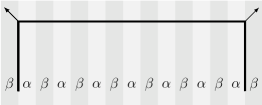
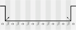
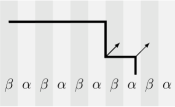
Figure 5. The calibrable edges in Propositions 3.7(i), 3.7(ii), and 3.4(ia)

Definition 3.8 ($\mathcal{C}$–edges).

We say that a horizontal edge $L=[p,q]\times\{\overline{y}\}$ is a $\mathcal{C}$–edge if is of one of the following types.

• $\chi_{L}=1,\ (p,\overline{y})\in\varepsilon\mathcal{I}_{\beta,\alpha},\ (q,\overline{y})\in\varepsilon\mathcal{I}_{\alpha,\beta}$.

• $\chi_{L}=-1,\ (p,\overline{y})\in\varepsilon\mathcal{I}_{\alpha,\beta},(q,\overline{y})\in\varepsilon\mathcal{I}_{\beta,\alpha}$.

• $\chi_{L}=0$, and either $n_{0}=1$, and $(p,\overline{y})$, $(q,\overline{y})\in\varepsilon\mathcal{I}_{\alpha,\beta}$, or $n_{0}=-1$, and $(p,\overline{y})$, $(q,\overline{y})\in\varepsilon\mathcal{I}_{\beta,\alpha}$.

By Propositions 3.4 and 3.7, every $\mathcal{C}$–edge is calibrable.

Remark 3.9 (Symmetric $\mathcal{C}$–edges).

When $L$ has positive $\varphi$–curvature, and $L=[-x_{N},x_{N}]\times\{\overline{y}\}$, with $\overline{y}\in\mathbb{R}$ and $x_{N}$ defined in (6), the velocity of $L$ is given by

(19) $$v_{L}=\frac{1}{x_{N}}+\frac{\alpha+\beta}{2}-\frac{(\beta-\alpha)\varepsilon}{8x_{N}}.$$

On the other hand, if $L$ has negative $\varphi$–curvature, and $L=[-x_{N}-\varepsilon/2,x_{N}+\varepsilon/2]\times\{\overline{y}\}$, setting $\overline{x}=x_{N}+\varepsilon/2$, the velocity of $L$ is given by

(20) $$v_{L}=-\frac{1}{\overline{x}}+\frac{\alpha+\beta}{2}+\frac{(\beta-\alpha)\varepsilon}{8\overline{x}}.$$

The general result concerning the long edges with positive $\varphi$–curvature is the following.

Proposition 3.10.

Let $L=[p,q]\times\{\overline{y}\}$ be a horizontal edge with positive $\varphi$–curvature, and such that $\ell+\ell_{\alpha}-\ell_{\beta}>4/(\beta-\alpha)$. Then the following hold.

• If either $g_{\varepsilon}(p)=\beta$, or $g_{\varepsilon}(q)=\beta$, or $p\in\varepsilon\mathcal{I}_{\alpha,\beta}$, or $q\in\varepsilon\mathcal{I}_{\beta,\alpha}$, then $L$ is not calibrable.

• If $g_{\varepsilon}(p)=g_{\varepsilon}(q)=\alpha$, let $\sigma_{1}$, $\sigma_{2}\in(0,\varepsilon/2)$ be such that $p+\varepsilon/2+\sigma_{1}\in\varepsilon\mathcal{I}_{\beta,\alpha}$ and $q-\varepsilon/2-\sigma_{2}\in\varepsilon\mathcal{I}_{\alpha,\beta}$, and let $\tilde{\ell}$ be the length of the interval $[p+\varepsilon/2+\sigma_{1},q-\varepsilon/2-\sigma_{2}]$. Setting

  $$m=\varepsilon\frac{\beta-\alpha}{(\beta-\alpha)(\tilde{\ell}+\varepsilon/2)+4},\qquad h=\frac{\varepsilon}{2}\frac{(\beta-\alpha)(\tilde{\ell}+\varepsilon/2)-4}{(\beta-\alpha)(\tilde{\ell}+\varepsilon/2)+4},$$

  and

  $$\Sigma=\left\{m\sigma_{2}+h\leq\sigma_{1}\leq\frac{1}{m}\sigma_{2}-\frac{h}{m}\right\},$$

  we have $m\in(0,1)$, $\Sigma\cap[0,\varepsilon/2]^{2}\neq\emptyset$, and $L$ is calibrable with velocity

  $$v_{L}=\frac{2}{\ell}+\frac{\alpha+\beta}{2}+\frac{\beta-\alpha}{2\ell}\left(\frac{\varepsilon}{2}-\sigma_{1}-\sigma_{2}\right)$$

  if and only if $(\sigma_{1},\sigma_{2})\in\Sigma$.

• if $g_{\varepsilon}(p)=\alpha$, and $q\in\varepsilon\mathcal{I}_{\alpha,\beta}$ (resp. $p\in\varepsilon\mathcal{I}_{\beta,\alpha}$, and $g_{\varepsilon}(q)=\alpha$), let $\sigma\in(0,\varepsilon/2)$ be such that $p+\sigma+\varepsilon/2\in\varepsilon\mathcal{I}_{\beta,\alpha}$, let $\ell^{*}$ be the length of the interval $[p+\varepsilon/2+\sigma,q]$ ( resp. of $[p,q-\varepsilon/2-\sigma]$), and let

  $$\sigma^{*}=\frac{\varepsilon}{2}\frac{(\beta-\alpha)(\ell^{*}+\varepsilon/2)-4}{(\beta-\alpha)(\ell^{*}-\varepsilon/2)+4}.$$

  Then $L$ is calibrable if and only if $\sigma\geq\sigma^{*}$.

Proof.

If $\ell+\ell_{\alpha}-\ell_{\beta}>4/(\beta-\alpha)$, by (13) the candidate Cahn–Hoffmann field $n$ is strictly decreasing in the $\beta$ phase. Hence, under the assumptions in (i), $n$ does not satisfy the constraint $|n|\leq 1$ at least near an endpoint, and $L$ is not calibrable.

Assume now that both the endpoints belong to the $\alpha$ phase, and let $\sigma_{1}$, $\sigma_{2}\in(0,\varepsilon/2)$ be such that $p+\varepsilon/2+\sigma_{1}\in\varepsilon\mathcal{I}_{\beta,\alpha}$ and $q-\varepsilon/2-\sigma_{2}\in\varepsilon\mathcal{I}_{\alpha,\beta}$. Then, by (13), we have

$$n(p+\varepsilon/2+\sigma_{1})-n(p)=\sigma_{1}\left(\frac{2}{\ell}+\frac{\beta-\alpha}{2\ell}(\ell+\ell_{\beta}-\ell_{\alpha})\right)+\frac{\varepsilon}{2}\left(\frac{2}{\ell}-\frac{\beta-\alpha}{2\ell}(\ell+\ell_{\alpha}-\ell_{\beta})\right).$$

In this case we have $\ell_{\beta}-\ell_{\alpha}=\varepsilon/2-\sigma_{1}-\sigma_{2}$, and $\ell=\tilde{\ell}+\varepsilon+\sigma_{1}+\sigma_{2}$, so that

$$\begin{split}n(p+\varepsilon/2+\sigma_{1})&-n(p)\\ &=\sigma_{1}\left(\frac{2}{\ell}+\frac{\beta-\alpha}{2\ell}\left(\tilde{\ell}+\frac{3}{2}\varepsilon\right)\right)+\frac{\varepsilon}{2}\left(\frac{2}{\ell}-\frac{\beta-\alpha}{2\ell}\left(\tilde{\ell}+\frac{\varepsilon}{2}+2\sigma_{1}+2\sigma_{2}\right)\right)\\ &=\frac{1}{2\ell}\left[\sigma_{1}\left(4+(\beta-\alpha)\left(\tilde{\ell}+\frac{\varepsilon}{2}\right)\right)+\frac{\varepsilon}{2}\left(4-(\beta-\alpha)\left(\tilde{\ell}+\frac{\varepsilon}{2}+2\sigma_{2}\right)\right)\right].\end{split}$$

Hence, if $\sigma_{2}\geq\sigma_{1}\geq m\sigma_{2}+h$, we have

$$n(q-\varepsilon/2-\sigma_{2})-n(q)\geq n(p+\varepsilon/2+\sigma_{1})-n(p)\geq 0,$$

and $n$ satisfies the constraint both in $[p,p+\varepsilon/2+\sigma_{1}]$ and in $[q-\varepsilon/2-\sigma_{2},q]$. By Remark 3.3, we obtain that $|n|\leq 1$ on $L$, and hence $L$ is calibrable. By symmetry, we obtain the same result when $\sigma_{1}\geq\sigma_{2}\geq m\sigma_{1}+h$, and the conclusion follows.

Finally, we have that $m\sigma_{2}+h=\sigma_{1}=\frac{1}{m}\sigma_{2}-\frac{h}{m}$ for $\sigma_{1}=\sigma_{2}=\tilde{\sigma}$, where

(21) $$\tilde{\sigma}:=\frac{\varepsilon}{2}\frac{(\beta-\alpha)(\tilde{\ell}+\varepsilon/2)-4}{(\beta-\alpha)(\tilde{\ell}-\varepsilon/2)+4},$$

and $\tilde{\sigma}\in(0,\varepsilon/2)$ under the assumption $\ell+\ell_{\alpha}-\ell_{\beta}>4/(\beta-\alpha)$, so that $\Sigma\cap[0,\varepsilon/2]^{2}\neq\emptyset$.

The proof of (iii) follows the same arguments. ∎

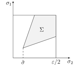
Figure 6. The calibrability set $\Sigma$ in Proposition 3.10

Remark 3.11 (Calibrability threshold).

In the special case when $\sigma_{1}=\sigma_{2}=\sigma>0$, Proposition 3.10(ii) implies that $L$ is calibrable if and only if $\sigma\geq\tilde{\sigma}$, where $\tilde{\sigma}$ is the quantity defined in (21). When $\sigma=\tilde{\sigma}$, the edge $L$ is calibrated by a Cahn–Hoffmann vector field $n$ such that $n(p)=n(p+\varepsilon/2+\tilde{\sigma})$ and $n(q)=n(q-\varepsilon/2-\tilde{\sigma})$. As a consequence, the same field calibrates both the edges $[p,p+\varepsilon/2+\tilde{\sigma}]\times\{\overline{y}\}$ and $[q-\varepsilon/2-\tilde{\sigma},q]\times\{\overline{y}\}$ (as edges with zero $\varphi$–curvature, see Proposition 3.4), and the edge $[p+\varepsilon/2+\tilde{\sigma},q-\varepsilon/2-\tilde{\sigma}]\times\{\overline{y}\}$ (as edges with positive $\varphi$–curvature, see Proposition 3.7) with the same velocity.

Similarly, in the case (iii) Proposition 3.10, when $\sigma=\sigma^{*}$, the edge $L$ is calibrated by a Cahn–Hoffmann vector field $n$ such that $n(p)=n(p+\varepsilon/2+\sigma^{*})$, and the same field calibrates both the edge $[p,p+\varepsilon/2+\sigma^{*}]\times\{\overline{y}\}$ (as edge with zero $\varphi$–curvature), and the edge $[p+\varepsilon/2+\tilde{\sigma},q]\times\{\overline{y}\}$ (as edges with positive $\varphi$–curvature) with the same velocity.

Remark 3.12 (Symmetric edges with positive $\varphi$–curvature).

If $L=[-\ell/2,\ell/2]\times\{\overline{y}\}$, $\ell>0$, $\overline{y}\in\mathbb{R}$, is a horizontal edge with positive $\varphi$–curvature, the previous results reed as follows. Setting $x_{N}=(N+1/4)\varepsilon$, $N\in\mathbb{N}$, let us define $\overline{N}_{\varepsilon}\in\mathbb{N}$ by

(22) $$\left(2x_{N}+\frac{\varepsilon}{2}\right)>\frac{4}{\beta-\alpha},\qquad\forall\ N\geq\overline{N}_{\varepsilon},$$

and $\delta(N)\in(0,\varepsilon)$ by

(23) $$\delta(N)=\dfrac{x_{N}(\beta-\alpha)\varepsilon}{2+\left(2x_{N}-\dfrac{\varepsilon}{2}\right)\dfrac{(\beta-\alpha)}{2}},$$

then $\delta(N)>\varepsilon/2$ if and only if $N\geq\overline{N}_{\varepsilon}$. Hence, if $\ell/2=x_{N_{\varepsilon}(\ell)}+\delta(\ell)$, with $0\leq\delta(\ell)<\varepsilon$, and

(24) $$N_{\varepsilon}(\ell)=\left\lfloor\dfrac{\ell}{2\varepsilon}-\dfrac{1}{4}\right\rfloor,$$

the following hold.

• If $N_{\varepsilon}(\ell)<\overline{N}_{\varepsilon}$, then the edge $L$ is calibrable.

• If $N_{\varepsilon}(\ell)\geq\overline{N}_{\varepsilon}$ then the edge $L$ is calibrable if and only if $\delta(\ell)\geq\delta(N_{\varepsilon}(\ell))$.

The analogous of Proposition 3.10 concerning the long edges with negative $\varphi$–curvature is the following.

Proposition 3.13.

Let $L=[p,q]\times\{\overline{y}\}$ be a horizontal edge with negative $\varphi$–curvature, and such that $\ell+\ell_{\beta}-\ell_{\alpha}>4/(\beta-\alpha)$. Then the following hold.

• If either $g_{\varepsilon}(p)=\alpha$, or $g_{\varepsilon}(q)=\alpha$, or $p\in\varepsilon\mathcal{I}_{\beta,\alpha}$, or $q\in\varepsilon\mathcal{I}_{\alpha,\beta}$, then $L$ is not calibrable.

• If $g_{\varepsilon}(p)=g_{\varepsilon}(q)=\beta$, let $\sigma_{1}$, $\sigma_{2}\in(0,\varepsilon/2)$ be such that $p+\varepsilon/2+\sigma_{1}\in\varepsilon\mathcal{I}_{\alpha,\beta}$ and $q-\varepsilon/2-\sigma_{2}\in\varepsilon\mathcal{I}_{\beta,\alpha}$, and let $\tilde{\ell}$ be the length of the interval $[p+\varepsilon/2+\sigma_{1},q-\varepsilon/2-\sigma_{2}]$.

  Then there exist $m\in(0,1)$ and $h>0$ such that $L$ is calibrable with velocity

  $$v_{L}=-\frac{2}{\ell}+\frac{\alpha+\beta}{2}-\frac{\beta-\alpha}{2\ell}\left(\frac{\varepsilon}{2}-\sigma_{1}-\sigma_{2}\right)$$

  if and only if $(\sigma_{1},\sigma_{2})\in\left\{m\sigma_{2}+h\leq\sigma_{1}\leq\frac{1}{m}\sigma_{2}-\frac{h}{m}\right\}$.

• if $g_{\varepsilon}(p)=\beta$, and $q\in\varepsilon\mathcal{I}_{\beta,\alpha}$ (resp. $p\in\varepsilon\mathcal{I}_{\alpha,\beta}$, and $g_{\varepsilon}(q)=\beta$), let $\sigma\in(0,\varepsilon/2)$ be such that $p+\sigma+\varepsilon/2\in\varepsilon\mathcal{I}_{\alpha,\beta}$, let $\ell^{*}$ be the length of the interval $[p+\varepsilon/2+\sigma,q]$ ( resp. of $[p,q-\varepsilon/2-\sigma]$), and let

  $$\sigma^{*}=\frac{\varepsilon}{2}\frac{(\beta-\alpha)(\ell^{*}+\varepsilon/2)-4}{(\beta-\alpha)(\ell^{*}-\varepsilon/2)+4}.$$

  Then $L$ is calibrable if and only if $\sigma\geq\sigma^{*}$.

4. Effective motion as $\varepsilon\to 0$

4.1. Evolution of rectangles

This section is devoted to the proof of the following result.

Theorem 4.1 (Effective motion of coordinate rectangles).

Let $R_{0}$ be a coordinate rectangle, and let $\ell_{1,0}$, $\ell_{2,0}$ be the length of its horizontal and vertical edges, respectively. For every $\varepsilon>0$, let $R_{0}^{\varepsilon}$ be a coordinate rectangle such that $d_{H}(R_{0},R_{0}^{\varepsilon})<\varepsilon.$ Then there exists a variational crystalline curvature flow of $R_{0}^{\varepsilon}$ with forcing term $g_{\varepsilon}$. Moreover, every variational crystalline curvature flow $E^{\varepsilon}(t)$ of $R_{0}^{\varepsilon}$ converges, in the Hausdorff topology and locally uniformly in time, as $\varepsilon\to 0$ to the coordinate rectangle $R(t)$ whose horizontal and vertical edges have lengths $\ell_{1}(t),\ell_{2}(t)$ solving the system of ODEs

(25) $$\begin{cases}\ell_{1}^{\prime}=-2\,H_{g}(\ell_{2}),\\ \ell_{2}^{\prime}=-\dfrac{4}{\ell_{1}}-(\alpha+\beta),\end{cases}$$

with initial datum $(\ell_{1}(0),\ell_{2}(0))=(\ell_{1,0},\ell_{2,0})$. The function $H_{g}(\ell)\colon(0,+\infty)\to\mathbb{R}$ is a truncation of the harmonic mean defined by

(26) $$H_{g}(\ell):=\begin{cases}0,&\text{if}\ \ell\geq-\dfrac{2}{\alpha},\\ \left\langle\dfrac{2}{\ell}+g\right\rangle=\dfrac{1}{\displaystyle\int_{0}^{1}\frac{1}{2/\ell_{2}+g(s)}\,ds}=\dfrac{(2+\alpha\ell_{2})(2+\beta\ell_{2})}{\ell_{2}\left(2+\dfrac{\alpha+\beta}{2}\ell_{2}\right)},&\text{otherwise}.\end{cases}$$

Remark 4.2.

If we assume that the evolution $E^{\varepsilon}(t)$ of a coordinate rectangle $R_{0}^{\varepsilon}$ is a coordinate rectangle for $t\in[0,T]$, and we denote by $(x_{1}(t),y_{1}(t))$, $(x_{2}(t),y_{1}(t))$, $(x_{2}(t),y_{2}(t))$, $(x_{1}(t),y_{2}(t))$, with $x_{1}(t)<x_{2}(t)$, and $y_{1}(t)>y_{2}(t)$, the coordinates of the vertices of $E^{\varepsilon}(t)$, the evolution of these points is governed by the system of ODEs’

(27) $$\begin{cases}x_{1}^{\prime}=\dfrac{2}{y_{1}-y_{2}}+g_{\varepsilon}(x_{1})\\[10.0pt] x_{2}^{\prime}=-\dfrac{2}{y_{1}-y_{2}}-g_{\varepsilon}(x_{2})\\[10.0pt] y_{1}^{\prime}=-\dfrac{2}{x_{2}-x_{1}}-\dfrac{\alpha+\beta}{2}-h_{\varepsilon}(y_{1},y_{2})\\[10.0pt] y_{2}^{\prime}=\dfrac{2}{x_{2}-x_{1}}+\dfrac{\alpha+\beta}{2}+h_{\varepsilon}(y_{1},y_{2})\end{cases}$$

in the domain $D:=\{(x_{1},x_{2},y_{2},y_{2})\colon x_{1}<x_{2},\ y_{1}>y_{2}\}$. The Lipshitz function $h_{\varepsilon}\colon\{y_{1}<y_{2}\}\subseteq\mathbb{R}^{2}\to\mathbb{R}$ takes into account the small reminder varying in $[-\varepsilon/2,\varepsilon/2]$ and appearing in (14).

Applying the classical results of differential equations with discontinouos right–hand side (see [22], Chapter 2), we obtain the following properties for the solutions.

• For every $P_{0}\in D$ there exists a (Filippov) solution to (27) starting from $P_{0}$.

• For every $P_{0}\in D\cap\{y_{1}-y_{2}\leq-2/\alpha\}$ there exists a unique local solution to (27) starting from $P_{0}$, and defined as long as it satisfies $y_{1}(t)-y_{2}(t)<-2/\alpha$.

• If $P_{0}\in D\cap\{y_{1}-y_{2}>-2/\alpha\}$, the uniqueness of the solution starting from $P_{0}$ fails if and only if either $x_{1}$ or $x_{2}$ belongs to the set of “unstable discontinuities” $U=\{\pm(x_{N}+\varepsilon/2),N\in\mathbb{N}\}$ (see (24) for the definition of $x_{N}$). If this does not occur, then the solution is unique until the first time $t_{0}$ for which either $x_{1}(t_{0})$ or $x_{2}(t_{0})$ belong to $U$.

• If $P_{0}\in D\cap\{y_{1}-y_{2}>-2/\alpha\}$, and $x_{1}$ (resp. $x_{2}$) belongs to the set of “stable discontinuities” $S=\{\pm x_{N},N\in\mathbb{N}\}$, then $x_{1}^{\prime}(t)=0$ (resp. $x_{2}^{\prime}(t)=0$) as long as the solution satisfies $y_{1}(t)-y_{2}(t)>-2/\alpha$.

Based on results of Section 3, a coordinate rectangle may not be calibrable, so that we cannot expect the evolution to preserve the geometry of the initial datum. In the proof of Theorem 4.1 we combine the previous properties of the solutions to (27) with a carefull description of why and how the geometry changes during the evolution.

Proof of Theorem 4.1.

We first assume that $R_{0}$ is centered at the origin. Using the notation

$$R(\ell_{1},\ell_{2})=\left[-\dfrac{\ell_{1}}{2},\dfrac{\ell_{1}}{2}\right]\times\left[-\dfrac{\ell_{2}}{2},\dfrac{\ell_{2}}{2}\right].$$

for this type of rectangles, $R_{0}=R(\ell_{1,0},\ell_{2,0})$.

We also assume that $R_{0}^{\varepsilon}=R(2x_{N_{\varepsilon}},\ell_{2,0})$, where ${N_{\varepsilon}}={N_{\varepsilon}}(\ell_{1,0})$ is defined in (24). In this case, recalling that the calibrability of a coordinate rectangle depends only on the calibrability of its horizontal edges (see Section 3.1), we have that $R_{0}^{\varepsilon}$ is calibrable (see Remark 3.9), and the evolution starts according to (27).

Case 1 (homogenized velocities): $\ell_{1,0}<4/(\beta-\alpha)$, $\ell_{2,0}\leq-2/\alpha$. The vertical edges of $R_{0}^{\varepsilon}=R(2x_{N_{\varepsilon}},\ell_{2,0}^{\varepsilon})$ are calibrable with velocity $v_{2}^{\varepsilon}(0)\geq 0$, and, by Remark 3.9, the horizontal edges are also calibrable with velocity

$$v_{1}^{\varepsilon}(0)=\frac{1}{x_{N_{\varepsilon}}}+\frac{\alpha+\beta}{2}+\frac{(\alpha-\beta)\varepsilon}{8x_{N_{\varepsilon}}}>0.$$

Then, by Section 3.1, Proposition 3.6, and Remark 4.2(ii), the (unique) evolution is given by shrinking coordinate rectangles $R(\ell_{1}^{\varepsilon}(t)),\ell_{2}^{\varepsilon}(t))$, and it is governed by system (27), or equivalently, by

(28) $$\begin{cases}{\ell_{1}^{\varepsilon}}^{\prime}=-\dfrac{4}{\ell_{2}^{\varepsilon}}-2g\left(\dfrac{\ell_{1}^{\varepsilon}}{\varepsilon}\right),\\[8.0pt] {\ell_{2}^{\varepsilon}}^{\prime}=-\dfrac{4}{\ell_{1}^{\varepsilon}}-(\alpha+\beta)-\dfrac{(\alpha-\beta)\varepsilon}{2\ell_{1}^{\varepsilon}}.\end{cases}$$

In order to pass to the limit as $\varepsilon\to 0^{+}$ and to find the effective evolution, notice that $\ell_{i}^{\varepsilon}\in(\ell_{i,\beta},\ell_{i,\alpha})$, $i=1,2$, where $(\ell_{1,\alpha},\ell_{2,\alpha})$ $(\ell_{1,\beta},\ell_{2,\beta})$ are the solution to (4) with initial datum $(2x_{N_{\varepsilon}},\ell_{2,0}^{\varepsilon})$, and forcing term $\gamma=\alpha$ and $\gamma=\beta$ respectively. Hence, for $T>0$, $\ell_{i}^{\varepsilon}$ are equilipschitz in $[0,T]$. Let $(\ell_{1}(t),\ell_{2}(t))$ the uniform limit of a suitable subsequence of $(\ell_{1}^{\varepsilon}(t)),\ell_{2}^{\varepsilon}(t))$ in [0,T]. Being a uniform limits of monotone non–increasing functions, $\ell_{i}(t)$ are non–increasing and hence differentiable almost everywhere in $[0,T]$. Moreover, for $t\in(0,T)$ and $\sigma>0$ such that $t+\sigma<T$, we have $\ell_{2}^{\varepsilon}(\tau)=\ell_{2}^{\varepsilon}(t)+O(\sigma)$ for $\tau\in[t,t+\sigma]$, and hence

$$\int_{\ell_{1}^{\varepsilon}(t)}^{\ell_{1}^{\varepsilon}(t+\sigma)}\dfrac{1}{2/\ell_{2}^{\varepsilon}(t)+g\left(s/\varepsilon\right)}\,ds+o(\sigma)=-2\sigma$$

and a passage to the limit as $\varepsilon\to 0$ gives

(29) $$\int_{\ell_{1}(t)}^{\ell_{1}(t+\sigma)}\frac{1}{\left\langle 2/\ell_{2}(t)+g\right\rangle}\,ds+o(\sigma)=-2\sigma$$

where $\langle 2/\ell_{2}+g\rangle$ is the harmonic mean of $2/\ell_{2}+g$ in $[0,1]$.

If $t$ is a differentiability point for $\ell_{1}$, from (29) it follows that $\ell_{1}^{\prime}(t)=-2\langle 2/\ell_{2}(t)+g\rangle$. In conclusion, the effective evolution of the rectangle $R(\ell_{1,0},\ell_{2,0})$ is given by rectangles $R(\ell_{1}(t),\ell_{2}(t))$ satisfying the evolution law

(30) $$\begin{cases}\ell_{1}^{\prime}=-2\left\langle\dfrac{2}{\ell_{2}}+g\right\rangle,\\[8.0pt] \ell_{2}^{\prime}=-\dfrac{4}{\ell_{1}}-(\alpha+\beta).\end{cases}$$

In this case all the edges move inwards until a finite extinction time.

Case 2 (mesoscopic pinning): $\ell_{2,0}\geq-2/\alpha$. By Section 3.1, the vertical edges of $R_{0}^{\varepsilon}=R(2x_{N_{\varepsilon}},\ell_{2,0})$ are calibrable with velocity $v_{2}^{\varepsilon}(0)=0$. Moreover, by Proposition 3.7, the horizontal edges of $R_{0}^{\varepsilon}=(x_{N_{\varepsilon}},\ell_{2,0})$ are also calibrable with velocity

$$v_{1}^{\varepsilon}(0)=\frac{1}{x_{N_{\varepsilon}}}+\frac{\alpha+\beta}{2}+\frac{(\alpha-\beta)\varepsilon}{8x_{N_{\varepsilon}}}.$$

If $v_{1}^{\varepsilon}(0)\leq 0$, then the length of the vertical edges does not decrease and the (unique) evolution at the mesoscopic scale is given by rectangles $R^{\varepsilon}(\ell_{1}^{\varepsilon}(t),\ell_{2}^{\varepsilon}(t))$, $t>0$, where

$$\begin{cases}{\ell_{1}^{\varepsilon}}^{\prime}=0,\\ {\ell_{2}^{\varepsilon}}^{\prime}=-\dfrac{2}{x_{N_{\varepsilon}}}-(\alpha+\beta)-\dfrac{(\alpha-\beta)\varepsilon}{4x_{N_{\varepsilon}}}.\end{cases}$$

Taking the limit as $\varepsilon\to 0$ we obtain that the effective evolution is given by $R(\ell_{1}(t),\ell_{2}(t))$, $t>0$, where

(31) $$\begin{cases}\ell_{1}^{\prime}=0,\\ \ell_{2}^{\prime}=-\dfrac{4}{\ell_{1,0}}-(\alpha+\beta).\end{cases}$$

Hence, if $\alpha+\beta<0$, the rectangles $R(-4/(\alpha+\beta),\ell_{2})$ with $\ell_{2,0}\geq-2/\alpha$ are unstable equilibria, while, if $v_{0}=4/\ell_{1,0}+(\alpha+\beta)<0$, the rectangle expands in the vertical direction with constant velocity $v_{0}$, keeping the length of the horizontal edges fixed.

If, instead, $v_{0}>0$, then the horizontal edges start to move inward, so that the length of the vertical edges decreases, and (31) describes the evolution for $t\in[0,\overline{t}]$, where

$$\overline{t}=\sup\{t>0\colon\ \ell_{2}(s))\geq-2/\alpha\ \forall s\in[0,t)\}.$$

Starting from $R(\ell_{1}(\overline{t}),-2/\alpha)$, the evolution is the one shown in Case 1 or 3, respectively.

Case 3 (mesoscopic breaking): $\ell_{1,0}\geq 4/(\beta-\alpha),\ \ell_{2,0}\leq-2/\alpha$. By Section 3.1, the vertical edges of $R_{0}^{\varepsilon}=R(2x_{N_{\varepsilon}},\ell_{2,0})$ are calibrable with velocity $v_{2}(0)\geq 0$, and, by Remark 3.9, the horizontal edges are calibrable with velocity

$$v_{1}^{\varepsilon}(0)=\frac{1}{x_{N_{\varepsilon}}}+\frac{\alpha+\beta}{2}+\frac{(\alpha-\beta)\varepsilon}{8x_{N_{\varepsilon}}}.$$

By Remark 3.12, the evolution is a rectangle, with decreasing length of the horizontal edges $\ell_{1}^{\varepsilon}(t)$, until the time $t_{\delta}>0$ such that $\ell_{1}^{\varepsilon}(t_{\delta})=2x_{N_{\varepsilon}}+2\delta(N_{\varepsilon}-1)$, where $\delta(N_{\varepsilon}-1)$ is the calibrability threshold given in (23). The horizontal edges of the rectangle cannot be calibrable after the time $t_{\delta}$. Nevertheless, by Remark 3.11, the Cahn–Hoffman vector field calibrating the horizontal edges at time $t_{\delta}$ equals the one calibrating separately the horizontal edges with positive $\varphi$–curvature

$$E_{c}^{\pm}:=[-x_{N_{\varepsilon}-1},x_{N_{\varepsilon}-1}]\times\{\pm\ell_{2}^{\varepsilon}(t_{\delta})/2\}$$

with velocity

$$v_{c}^{\varepsilon}=\frac{1}{x_{N_{\varepsilon}-1}}+\frac{\alpha+\beta}{2}+\frac{(\alpha-\beta)\varepsilon}{8x_{N_{\varepsilon}-1}},$$

and the horizontal edges with zero curvature

$$\begin{split}E_{l}^{\pm}&:=\left[\frac{-\ell_{1}(t_{\delta})}{2},-x_{N_{\varepsilon}-1}\right]\times\left\{\pm\frac{\ell_{2}^{\varepsilon}(t_{\delta})}{2}\right\}\\ E_{r}^{\pm}&:=\left[x_{N_{\varepsilon}-1},\frac{\ell_{1}(t_{\delta})}{2}\right]\times\left\{\pm\frac{\ell_{2}^{\varepsilon}(t_{\delta})}{2}\right\}\end{split}$$

with the same velocity (see Figure 7).

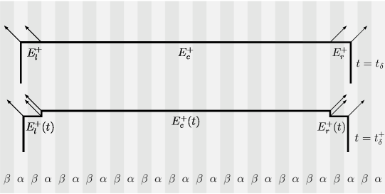
Figure 7. Breaking of the horizontal edge at $t=t_{\delta}$.

Hence, the Cahn–Hoffman vector field $n(t)$ evolves continuously after $t_{\delta}$ by breaking the horizontal edges into three parts, that we denote by $E_{l}^{\pm}(t)$, $E_{c}^{\pm}(t)$ and $E_{r}^{\pm}(t)$ respectively, and the evolution becomes a coordinate polyrectangle $P^{\varepsilon}(t)$ (see Figure 7).

By symmetry, the lengths and the velocities of the edges $E_{l}^{\pm}(t)$, $E_{c}^{\pm}(t)$ are the same; they will be denoted by $\ell_{h}^{\varepsilon}(t)$ and $v_{h}^{\varepsilon}(t)$, respectively.

By Section 3.1 the small vertical edges with zero $\varphi$–curvature are pinned on the interfaces $x=\pm x_{N_{\varepsilon}-1}$, so that, by Remark 3.9, the long horizontal edges with positive $\varphi$–curvature $E_{c}^{\pm}(t)$ have constant length $\ell_{1}^{\varepsilon}=2x_{N_{\varepsilon}-1}$, and move with velocity $v_{1}^{\varepsilon}(t)=v_{c}^{\varepsilon}$.

By Remark 3.5, the small horizontal edges $E_{l}^{\pm}(t)$ and $E_{c}^{\pm}(t)$ with zero $\varphi$–curvature and length $\ell_{h}^{\varepsilon}(t)\in(0,\varepsilon/2+\delta(N_{\varepsilon}))$ move with velocity $v_{h}^{\varepsilon}(t)>v_{c}^{\varepsilon}(t)$ given by

$$v_{h}^{\varepsilon}(t)=\begin{cases}\beta&\text{if}\ \ell_{h}^{\varepsilon}(t)\in(0,\varepsilon/2)\\[6.0pt] \dfrac{1}{\ell_{h}^{\varepsilon}(t)}\left(\dfrac{\varepsilon}{2}\beta+\left(\ell_{h}^{\varepsilon}(t)-\dfrac{\varepsilon}{2}\right)\alpha\right)&\text{if}\ \ell_{h}^{\varepsilon}(t)\in(\varepsilon/2,\varepsilon)\end{cases}$$

reducing the length $\ell_{2}^{\varepsilon}(t)$ of the long vertical edges with positive $\varphi$–curvature

$$\ell_{2}^{\varepsilon}(t)=\ell_{2}^{\varepsilon}(t_{\delta})-\int_{t_{\delta}}^{t}v_{h}^{\varepsilon}(s)\,ds\leq\ell_{2}^{\varepsilon}(t_{\delta})-v_{c}^{\varepsilon}(t-t_{\delta}).$$

On the other hand, the vertical long edges with positive $\varphi$–curvature move inward with velocity

$$v_{2}^{\varepsilon}(t)=\frac{2}{\ell_{2}^{\varepsilon}(t)}+g_{\varepsilon}\geq\frac{2}{\ell_{2}^{\varepsilon}(t_{\delta})-v_{c}^{\varepsilon}(t-t_{\delta})}+\alpha$$

so that, if we denote by $t_{1}$ the time when the vertical long edges with positive $\varphi$–curvature reach the interfaces $x=\pm x_{N_{\varepsilon}-1}$, we obtain

$$2\varepsilon\geq\int_{t_{\delta}}^{t_{1}}\frac{2}{\ell_{2}^{\varepsilon}(t_{\delta})-v_{c}^{\varepsilon}(t-t_{\delta})}\,dt+\alpha(t_{1}-t_{\delta})\geq\left(\frac{2}{\ell_{2}^{\varepsilon}(t_{\delta})}+\alpha\right)(t_{1}-t_{\delta}).$$

Hence, at $t=t_{1}$ the evolution is a rectangle $R(x_{N_{\varepsilon}-1},\ell_{2}^{\varepsilon}(t_{1}))$ where

$$\ell_{2}^{\varepsilon}(t_{1})=\ell_{2}^{\varepsilon}(t_{\delta})-v_{c}^{\varepsilon}(t_{1}-t_{\delta})=\ell_{2}^{\varepsilon}(t_{\delta})+O(\varepsilon),\quad\varepsilon\to 0^{+}.$$

The (unique) evolution then iterates this “breaking and recomposing” motion in such a way that it can be approximate, in Hausdorff topology and locally uniformly in time, by a family of rectangles $R(\tilde{\ell}_{1}^{\varepsilon}(t),\tilde{\ell}_{2}^{\varepsilon}(t))$ satisfying (28), so that the effective motion is a family of rectangles $R(\ell_{1}(t),\ell_{2}(t))$ governed by the evolution law (30).

The general results recalled in Remark 4.2 can be used to show that the effective evolution (25) does not depend on the choiche of the approximating sequence $R_{0}^{\varepsilon}$ of initial data.

Namely, in Case 1, any coordinate rectangle $R_{0}^{\varepsilon}$ is calibrable and the (unique) evolution starting from $R_{0}^{\varepsilon}$ is the family of coordinate rectangles solving (27). This evolution has a distance of order $\varepsilon$ from the one starting from $R(2x_{N_{\varepsilon}},\ell_{2,0})$ uniformly in time, so that it converges, as $\varepsilon\to 0^{+}$ to the same effective evolution.

Similarly, in Case 3, we have that the evolution starting from $R_{0}^{\varepsilon}$ becomes a rectangle with vertical edges with left endpoint on $\varepsilon\mathcal{I}_{\beta,\alpha}$ and right endpoint on $\varepsilon\mathcal{I}_{\alpha,\beta}$ in a time span of order $\varepsilon$, possibly breaking and recomposing the horizontal edges in the meanwhile. Then, the effective evolution of $R_{0}$ is uniquely determined by (30).

On the other hand, if $\ell_{2,0}>-2/\alpha$, then, by Remark 4.2(iii) and (iv), the position of the vertical edges during the evolution is confined in the strip $\{x\in[x_{N_{\varepsilon}-1},x_{N_{\varepsilon}}]\}$, with $N_{\varepsilon}=N_{\varepsilon}(\ell_{1,0}^{\varepsilon})$. Hence, at a macroscopic level, the vertical edges are pinned, and the effective evolution of $R_{0}$ is uniquely determined by (31).

∎

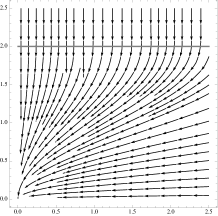
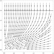
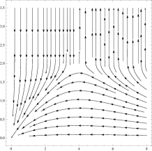
Figure 8. Phase portraits of (25) for $\alpha+\beta=0$ (left), $>0$ (center), $<0$ (right)

System (25) is integrable, and its phase portrait is plotted in Figure 8. Notice the pinning effect for long vertical edges, and the presence of a half line of nontrivial equilibria for $\alpha+\beta<0$.

Remark 4.3 (Partial uniqueness of the forced crystalline curvature flow).

We emphasize that, in the proof of Theorem 4.1, we have shown that the forced crystalline curvature flow starting from a coordinate rectangle of the type $R_{0}^{\varepsilon}=R(2x_{N_{\varepsilon}},\ell_{2,0})$ is unique. The uniqueness of the solution is essentially based on Remark 4.2(iii) and (iv), and it holds for the evolution starting from any coordinate rectangle with horizontal $\mathcal{C}$–edges (recall Definition 3.8). Namely, by Remark 4.2(iii), uniqueness may fail if and only if the evolution has a “long” vertical edge on a unstable discontinuity, but this is not the case, because the evolution from a coordinate rectangle with horizontal $\mathcal{C}$–edges has pinned “long” vertical edges (see also Proposition 4.8 below).

4.2. Evolution of polyrectangles

We now extend the previous results to the more general class of coordinate polyrectangles, that is those sets whose boundary is a closed polygonal curve with edges parallel to the coordinate axes.

Given a coordinate polyrectangle $E$, in what follows we will denote by $H^{0}$, $H^{+}$, and $H^{-}$ (respectively $V^{0}$, $V^{+}$, and $V^{-}$) the sets of the horizontal (resp. vertical) edges of $\partial E$ with zero, positive and negative $\varphi$–curvature. Moreover we set $H=H^{0}\cup H^{+}\cup H^{-}$, and $V=V^{0}\cup V^{+}\cup V^{-}$.

In what follows $\ell$ will denote the length of the edge $L$.

Remark 4.4.

Given a coordinate polyrectangle $E$, the description of the variational crystalline curvature flow $E^{\varepsilon}(t)$ with forcing term $g_{\varepsilon}$ starting from $E$ will be obtained by combining the calibrability properties of the edges proved in Section 3 and information about solutions of a coupled system of ODEs solved by the coordinates of the vertices of $E(t)$ in any interval $I$ in which the number of vertices of $E^{\varepsilon}(t)$ does not change.

More precisely, let $(x_{i}(t),y_{i}(t))$, $i=1,\ldots,N$, be the coordinates of the vertices of the polyrectangles $E^{\varepsilon}(t)$, $t\in I$, ordered clockwise in such a way that

$$(x_{1},y_{1})=(x_{N+1},y_{N+1}),\quad x_{2k}(t)=x_{2k+1}(t),\ y_{2k}(t)=y_{2k-1}(t),\quad k=1,\ldots,\frac{N}{2},\ t\in I,$$

and the edges of $E^{\varepsilon}(t)$ are given by

$$L_{i}(t)=\begin{cases}[x_{i}(t),x_{i+1}(t)]\times\{y_{i}\}&\text{for $i$ odd}\\ \{x_{i}\}\times[y_{i}(t),y_{i+1}(t)]&\text{for $i$ even}.\end{cases}$$

Then $(x_{1}(t),\ldots,x_{N}(t),y_{1}(t),\ldots,y_{N}(t))$ is a solution in $I$ to the system of ODEs

(32) $$\begin{cases}x_{2k}^{\prime}=x_{2k+1}^{\prime}=-\dfrac{2}{y_{2k}-y_{2k+1}}{\chi}_{L_{2k}}-g_{\varepsilon}(x_{2k})\\[10.0pt] y_{2k}^{\prime}=y_{2k+1}^{\prime}=-\dfrac{1}{x_{2k}-x_{2k-1}}\left(2{\chi}_{L_{2k-1}}+\displaystyle\int_{x_{2k-1}}^{x_{2k}}g_{\varepsilon}(s)\,ds\right)\end{cases}\quad k=1,\ldots\frac{N}{2}.$$

The velocity field in (32) is discontinuous on the set

$$\mathcal{D}:=\{(x_{1},\ldots,x_{N},y_{1},\ldots,y_{N})\ \text{such that}\ \exists i=1,\ldots,N\colon\ x_{i}\in\varepsilon\mathcal{I}\},$$

so that the discontinuities only affect the motion of the vertical edges. We collect here the main features of the solutions to (32) (see [22], Chapter 2), written in terms of motion of the edges of $\partial E^{\varepsilon}(t)$, $t\in I$. Since the system (32) is autonomous, it is enough to discuss the properties of local solutions starting from given datum $E$.

• Pinning effect (stable discontinuities). Let $\ell_{p}>0$ be the pinning threshold defined by

  $$\ell_{p}=\begin{cases}-\dfrac{2}{\alpha},&\text{if}\ L\in V^{+},\\[4.0pt] 0,&\text{if}\ L\in V^{0},\\[4.0pt] \dfrac{2}{\beta},&\text{if}\ L\in V^{-}.\end{cases}$$

  Then every vertical edge $L\in\partial E$ with $\ell>\ell_{p}$ and such that either $\nu(L)=e_{1}$ and $L\in\varepsilon\mathcal{I}_{\beta,\alpha}$ or $\nu(L)=-e_{1}$ and $L\in\varepsilon\mathcal{I}_{\alpha,\beta}$ is pinned during the evolution $E^{\varepsilon}(t)$ for every $t>0$ such that $\ell(t)\geq\ell_{p}$.

• Trasversality condition. The motion of a vertical edge $L\in V^{-}\cup V^{+}$ with $\ell<\ell_{p}$ is uniquely determined until $\ell(t)<\ell_{p}$.

• Uniqueness condition (unstable discontinuities). The uniqueness of the local solution starting from $E$ fails if and only if there is a vertical edge $L\in V^{-}\cup V^{+}$ with $\ell>\ell_{p}$ and such that either $\nu(L)=e_{1}$ and $L\in\varepsilon\mathcal{I}_{\alpha,\beta}$ or $\nu(L)=-e_{1}$ and $L\in\varepsilon\mathcal{I}_{\beta,\alpha}$ (unstable edges). If this does not occur, the solution is unique until the first time $t_{0}$ when $E^{\varepsilon}(t_{0})$ has a unstable edge.

A significant class of coordinate polyrectangles with a well posed forced evolution is the following (see Proposition 4.8 and Theorem 4.9 below).

Definition 4.5 ($\mathcal{C}$–polyrectangles).

Given $\varepsilon>0$, we say that a coordinate polyrectangle $E$ is a $\mathcal{C}$–polyrectangle if every horizontal edge of $E$ is a $\mathcal{C}$–edge (see Definition 3.8).

Remark 4.6.

By Proposition 3.7, Proposition 3.4, and Remark 4.4, every $\mathcal{C}$-polyrectangle is calibrable, with velocity of an edge $L$ given by

(33) $$v_{L}=\begin{cases}\dfrac{\alpha+\beta}{2}+\chi_{L}\left(\dfrac{2}{\ell}-\dfrac{(\beta-\alpha)\varepsilon}{4\ell}\right),&L\in H\\[6.0pt] \dfrac{2}{\ell}\chi_{L}+\gamma_{\varepsilon},&L\in V^{+}\cup V^{-},\ \ell<\ell_{p}\\[6.0pt] 0,&\text{$L\in V^{0}$, and $L\in V^{-}\cup V^{+}$ with $\ell\geq\ell_{p}$.}\end{cases}$$

(see Figure 9), and the variational crystalline curvature flow with forcing term $g_{\varepsilon}$ of $E$ starts following the rules (32). In particular, every edge $L\in V^{0}$ is pinned, as well as any edge $L\in V^{-}\cup V^{+}$ with length $\ell\geq\ell_{p}$.

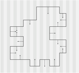
Figure 9. A $\mathcal{C}$–polyrectangle with velocities of its edges (case $\alpha+\beta>0$)

Theorem 4.7 (Effective motion of coordinate polyrectangles).

Let $E_{0}$ be a coordinate polyrectangle. For $\varepsilon>0$, let $E_{0}^{\varepsilon}$ be a coordinate polyrectangle such that $d_{H}(E_{0},E_{0}^{\varepsilon})<\varepsilon$. Then there exists a variational crystalline curvature flow with forcing term $g_{\varepsilon}$ starting from $E_{0}^{\varepsilon}$. Moreover, there exists a family of coordinate polyrectangles $E(t)$ such that every variational crystalline curvature flow $E^{\varepsilon}(t)$ with forcing term $g_{\varepsilon}$ of $E_{0}^{\varepsilon}$ converges to $E(t)$ in the Hausdorff topology and locally uniformly in $t$, for $\varepsilon\to 0$.

Denoting by $\ell(t)$ the length of an edge $L(t)\subseteq\partial E(t)$, the normal velocity $v_{L}(t)$ of $L(t)$ is given by

(34) $$v_{L}(t)=\begin{cases}\,\left\langle g+\dfrac{2}{\ell(t)}\right\rangle,&\text{if $L(t)\in V^{+}$, and}\ \ell(t)<-2/\alpha,\\[8.0pt] \,\left\langle g-\dfrac{2}{\ell(t)}\right\rangle,&\text{if $L(t)\in V^{-}$, and}\ \ell(t)<2/\beta,\\[8.0pt] \phantom{-}0,&\text{for the other vertical edges,}\\[4.0pt] \dfrac{2}{\ell(t)}\chi_{L}+\dfrac{\alpha+\beta}{2},&\text{if $L(t)$ is horizontal.}\end{cases}$$

The dynamics (34) is valid until $\ell(t)>0$. If an edge vanishes at $t=t_{0}$, the evolution proceedes reinitializing the ODEs by starting from $E(t_{0})$.

Proof.

The existence of a variational crystalline curvature flow with forcing term $g_{\varepsilon}$ starting from a coordinate polyrectangle $E^{\varepsilon}_{0}$ and the fact that the effective evolution does not depend on the choice of the approximating data can be obtained with arguments similar to the ones proposed in detail in Section 4.1. We roughly sketch here the main features of such an evolution starting from a $\mathcal{C}$–polyrectangle $E^{\varepsilon}_{0}$.

By Remark 4.6, the “long” vertical edges of $\partial E^{\varepsilon}_{0}$ with non zero $\varphi$–curvature, and all the vertical edges with zero $\varphi$–curvature are pinned. The vertical edges in $V^{+}$ with length $\ell<-2/\alpha$ move inward, while the vertical edges in $V^{-}$ with length $\ell<2/\beta$ move outward.

By Proposition 3.4, every edge $L\in H^{0}$ with pinned vertices has velocity $(\alpha+\beta)/2$, while every edge $L\in H^{0}$ with an adjacent moving vertical edge breaks istantaneously in a small part $L_{\varepsilon}$ with length $\varepsilon$, and a remaining part calibrated with velocity $(\alpha+\beta)/2$. During the evolution $L_{\varepsilon}$ shrinks and disappears in a time of order $\varepsilon$, while the remaing part has pinned vertices and moves vertically with velocity $(\alpha+\beta)/2$.

Similarly, every edge $L\in H^{+}\cup H^{-}$ with pinned vertices has velocity given by (33), while every edge $L\in H^{+}\cup H^{-}$ with an adjacent moving vertical edge shrinks until the calibrability conditions of Propositions 3.10 and 3.13 hold, and possibly it breaks following the rules of Remark 3.11.

In any case, the possible “breaking and recomposing” motion occurs in a lapse of time of order $\varepsilon$, so that the evolution $E^{\varepsilon}(t)$ can be approximated by a family of $\mathcal{C}$–polirectangles $\tilde{E}^{\varepsilon}(t)$ converging as $\varepsilon\to 0$ to a coordinate polyrectangle $E(t)$ in Hausdorff topology and locally uniformly in time. The effective velocities (34) of the edges of $E(t)$ are obtained taking the limit, as $\varepsilon\to 0$ in (33). In particular, the arguments for getting the velocities of the “short” vertical edges are the same of Case 1 in Section 4.1. ∎

The variational crystalline curvature flow with forcing term $g_{\varepsilon}$ starting from a $\mathcal{C}$–polyrectangle is unique and satisfies a comparison principle.

Proposition 4.8 (Uniqueness).

Given $\varepsilon>0$, the variational crystalline curvature flow $E^{\varepsilon}(t)$ with forcing term $g_{\varepsilon}$ starting from a $\mathcal{C}$–polyrectangle $E$ is unique.

Proof.

By Remark 4.4(iii), uniqueness may fail if and only if there exists $t_{0}>0$ such that $\partial E(t_{0})$ has a unstable edge. We will show that this never occurs when the initial datum $E$ is a $\mathcal{C}$–polyrectangle.

By Remarks 4.4 and 4.6, the evolution starts with all the vertical edges pinned on interfaces in $\varepsilon\mathcal{I}$ that are stable equilibria of the dynamics, except for the “short” edges with nonzero $\varphi$–curvature. Moreover, the evolution may generate, for $t>0$ new vertical edges, due to the breaking phenomenon of the horizontal edges. Nevertheless, every new vertical edge $L$ belongs to $V^{0}$ and it is pinned on a stable discontinuity of $g_{\varepsilon}$.

Hence, if we assume by contraddiction that there exists $t_{0}>0$ such that $\partial E(t_{0})$ has a unstable edge, then it is the evolution $L(t_{0})$ of a “short” edge (that is $L\in V^{-}\cup V^{+}$ with $\ell<\ell_{p}$) enlarging during the evolution. More precisely, if we assume that $L(t_{0})\in V^{+}$ and $\nu(L(t_{0}))=e_{1}$ (the other cases being similar), the following properties should be satisfied:

$$L(t_{0})\in\varepsilon\mathcal{I}_{\alpha,\beta},\quad\ell(t_{0})>-2/\alpha,$$

and there exists $\sigma>0$ such that

$$g_{\varepsilon}=\alpha\ \text{on}\ L(t)\ \text{for}\ t\in(t_{0}-\sigma,t_{0}),\quad\ell(t_{0}-\sigma)<-2/\alpha\ .$$

Since $\partial E(t_{0})$ needs to be calibrable, the horizontal edges adjacent to $L(t_{0})$ have either zero $\varphi$–curvature, length $\varepsilon/2$ and velocity $\beta$, or positive $\varphi$–curvature, and length satisfying $\ell+\ell_{\alpha}-\ell_{\beta}\leq 4/(\beta-\alpha)$ (see Proposition 3.6), and hence velocity

$$v=\frac{2}{\ell}+\frac{\alpha+\beta}{2}+\frac{\beta-\alpha}{2\ell}(\ell_{\beta}-\ell_{\alpha})=\frac{1}{2\ell}(4-(\beta-\alpha)(\ell+\ell_{\alpha}-\ell_{\beta})+2\beta\ell)>0.$$

In both cases the horizontal edges adjacent to $L(t_{0})$ have strictly positive velocity, in contraddiction with the fact that $L(t)$ enlarges for $t<t_{0}$ close enought to $t_{0}$. ∎

Theorem 4.9 (Comparison for forced flows).

For a given $\varepsilon>0$, let $E$ and $F$ be two $\mathcal{C}$–polyrectangles such that $E\subseteq F$, and let $E^{\varepsilon}(t)$, $F^{\varepsilon}(t)$ be the variational crystalline curvature flow of $E$ and $F$, respectively, with forcing term $g_{\varepsilon}$. Then

• $E^{\varepsilon}(t)\subseteq F^{\varepsilon}(t)$ for every $t$.

• the distance $d^{\varepsilon}(t)$ between $\partial E^{\varepsilon}(t)$ and $\partial F^{\varepsilon}(t)$ satisfies

  $$d^{\varepsilon}(t)\geq d^{\varepsilon}(0)\quad\forall t\geq 0,\qquad\text{and}\qquad d^{\varepsilon}(t_{1})\geq d^{\varepsilon}(t_{2})-\varepsilon\quad\forall t_{1}\geq t_{2}>0.$$

Proof.

Given $\sigma>0$, let $E^{\varepsilon}_{\sigma}(t)$ be the variational crystalline curvature flow of $E$ with forcing term $g_{\varepsilon}+\sigma$. Following the proof of the First Comparison Principle in [25], mainly based on geometric arguments, we obtain that $E^{\varepsilon}_{\sigma}(t)\subseteq F^{\varepsilon}(t)$.

Moreover, by Theorem 4.7, Proposition 4.8, and Theorem 2.8.2 in [22], we infer that for every $n\in\mathbb{N}$ there exists $\sigma_{n}>0$ such that, for every $t>0$, the evolutions $E^{\varepsilon}_{\sigma_{n}}(t)$ converge, as $n\to+\infty$, in Hausdorff topology to the variational crystalline curvature flow $E^{\varepsilon}(t)$ with forcing term $g_{\varepsilon}$ starting from $E$. Hence (i) follows from a passage to the limit for the inclusions $E^{\varepsilon}_{\sigma_{n}}(t)\subseteq F^{\varepsilon}(t)$.

In order to prove (ii), we underline that for every $t>0$ the minimal distance $d(t)$ between $\partial E^{\varepsilon}(t)$ and $\partial F^{\varepsilon}(t)$ is attained at points joined by a segment parallel to a coordinate axis, so that either $E(t)+d(t)e_{1}\subseteq F(t)$ or $E(t)+d(t)e_{2}\subseteq F(t)$. On the other hand, since $E$ is a $\mathcal{C}$–polyrectangle, we have that, for every $\gamma\in\mathbb{R}$, $E^{\varepsilon}(t)+\gamma e_{2}$ is the variational crystalline curvature flow with forcing term $g_{\varepsilon}$ starting from $E+\gamma\,e_{2}$, and, for every $k\in\mathbb{Z}$, $E^{\varepsilon}(t)+k\varepsilon e_{1}$ is the variational crystalline curvature flow with forcing term $g_{\varepsilon}$ starting from $E+k\varepsilon\,e_{1}$.

Let $t_{1}\geq 0$ be given. If $E(t_{1})+d(t_{1})e_{2}\subseteq F(t_{1})$, then, by (i) and the invariance of the flow under vertical translations, we have that $E(t)+d(t_{1})e_{2}\subseteq F(t)$, and hence $d^{\varepsilon}(t_{1})\geq d^{\varepsilon}(t)$, for every $t\geq t_{1}$. If, instead, $E(t_{1})+d(t_{1})e_{1}\subseteq F(t_{1})$, with the same argument we obtain that (ii) holds and that $d^{\varepsilon}(t_{1})\geq d^{\varepsilon}(t)$ for every $t\geq t_{1}$ if and only if $d(t_{1})=k\varepsilon$.

∎

4.3. Evolution of more general sets

The macroscopic effect of the underlying oscillating forcing term $g_{\varepsilon}$ on the crystalline curvature flow starting from any smooth, connected bounded set $C_{0}$ may be captured in the following way.

For every $\varepsilon>0$, let $\mathcal{C}_{\varepsilon}$ be the set of all $\mathcal{C}$–polyrectangles. For every $E_{\varepsilon}(0)\in\mathcal{C}_{\varepsilon}$, let $E_{\varepsilon}(t)$ be the unique variational crystalline curvature flow with forcing term $g_{\varepsilon}$ starting from $E_{\varepsilon}(0)$. We define the families of sets

$$C^{+}_{\varepsilon}(t)=\bigcap_{\begin{subarray}{c}C_{0}\subseteq P_{\varepsilon}(0)\\ P_{\varepsilon}(0)\in\mathcal{C}_{\varepsilon}\end{subarray}}P_{\varepsilon}(t),\qquad C^{-}_{\varepsilon}(t)=\bigcup_{\begin{subarray}{c}Q_{\varepsilon}(0)\subseteq C_{0}\\ Q_{\varepsilon}(0)\in\mathcal{C}_{\varepsilon}\end{subarray}}Q_{\varepsilon}(t),$$

and

$$\begin{split}C^{+}(t)&=\limsup_{\varepsilon\to 0^{+}}C^{+}_{\varepsilon}(t)=\bigcap_{\eta>0}\left(\bigcup_{0<\varepsilon<\eta}C^{+}_{\varepsilon}(t)\right),\\ C^{-}(t)&=\liminf_{\varepsilon\to 0^{+}}C^{-}_{\varepsilon}(t)=\bigcup_{\eta>0}\left(\bigcap_{0<\varepsilon<\eta}C^{-}_{\varepsilon}(t)\right).\end{split}$$

By Theorem 4.9, for every $P_{\varepsilon}(0)$, $Q_{\varepsilon}(0)\in\mathcal{C}_{\varepsilon}$ such that $Q_{\varepsilon}(0)\subseteq C_{0}\subseteq P_{\varepsilon}(0)$, the evolutions satisfy $Q_{\varepsilon}(t)\subseteq P_{\varepsilon}(t)$ for every $t\geq 0$. Hence we have $C^{-}_{\varepsilon}(t)\subseteq C^{+}_{\varepsilon}(t)$, $t\geq 0$.

Moreover, denoting by $P(t),Q(t)$ the effective evolution starting from coordinate polyrectangles $P(0),Q(0)$, and evolving with the law (34), by Theorem 4.7 we obtain that

$$\bigcup_{Q(0)\subseteq C_{0}}Q(t)\subseteq C^{-}(t)\subseteq C^{+}(t)\subseteq\bigcap_{C_{0}\subseteq P(0)}P(t),\qquad t\geq 0.$$

Notice that $C^{-}(0)=C^{+}(0)=C_{0}$. When $C^{-}(t)=C^{+}(t)=:C(t)$ for $t>0$, this procedure defines the limit evolution starting from $C_{0}$ and driven, at a mesoscopic scale, by crystalline curvature flow with forcing term $g_{\varepsilon}$.

If $C_{0}$ is a bounded convex subset of $\mathbb{R}^{2}$ with nonempty interior, then $C^{-}(t)=C^{+}(t)$ for all $t\geq 0$, and we can explicitely describe the motion $C(t)$ starting from $C_{0}$.

Approximation far from the ”extreme points”: constant vertical shift. Let $\xi\in\partial C_{0}$ be such that $\nu(\xi)$ is not a coordinate vector. In this case, we can choose approximating sequences of $\mathcal{C}$–polyrectangles with all edges with zero $\varphi$–curvature in a suitable neighborhood of $\xi$ (see Figure 10, left). The evolution by (34) of such an approximation is the following: the vertical edges are pinned, while the horizontal edges moves with velocity $(\alpha+\beta)/2$. At a macroscopic level, the effect is a vertical motion of $\partial C_{0}$ near $\xi$ with velocity $(\alpha+\beta)/2$ .

Figure 10. Approximation far from (left) and near to (right) an extreme point

Approximation near the ”extreme points”: flat evolution. Let $\xi\in\partial C_{0}$ be such that $\nu(\xi)=\pm e_{1}$. In this case, we can choose approximating sequences of $\mathcal{C}$–polyrectangles with one horizontal edge with positive $\varphi$–curvature in a suitable neighborhood of $\xi$. Then the evolution $C(t)$, $t>0$, has a horizontal edge $L(t)$ with length $l(t)$ moving vertically with velocity $2/\ell(t)+(\alpha+\beta)/2$. The same arguments show that the evolution $C(t)$, $t>0$, has flat vertical edges “generated by” the points $\xi\in\partial C_{0}$ be such that $\nu(\xi)=\pm e_{2}$ and moving horizontally with velocity $H_{g}(\ell(t))$ (see (26)).

In conclusion, the effective evolution $C(t)$ of a convex set $C_{0}$ can be depicted as follows.

• The arcs with zero $\varphi$–curvature moves vertically with velocity $(\alpha+\beta)/2$. Let us denote by $C_{1}(t)$, the set obtained with this translation.

• There is an instantaneous generation of four flat edges parallel to the coordinate axes and with the extreme points constrained on the set $C_{1}(t)$. The horizontal edges moves vertically with velocity $2/\ell+(\alpha+\beta)/2$, while the vertical ones moves horizontally with velocity $H_{g}(\ell(t))$.

For example, the effective evolution starting from a circle is depicted in Figure 11.

Figure 11. Effective evolution of a circle.

References

- [1] F. Almgren and J.E. Taylor. Flat flow is motion by crystalline curvature for curves with crystalline energies. J. Differential Geometry 42 (1995), 1–22.
- [2] F. Almgren, J.E. Taylor, L.H. Wang. Curvature–driven flows: a variational approach. SIAM J. Control Optim. 31 (1993), 387–438.
- [3] L. Ambrosio and A. Braides. Functionals defined on partitions of sets of finite perimeter, I: integral representation and -convergence. J. Math. Pures. Appl. 69 (1990), 285-305.
- [4] L. Ambrosio, N. Gigli, and G. Savaré. Gradient Flows in Metric Spaces and in the Space of Probability Measures. Lectures in Mathematics ETH, Zürich. Birkhhäuser, Basel, 2008.
- [5] G. Bellettini, R. Goglione, M. Novaga. Approximation to driven motion by crystalline curvature in two dimensions. Adv. Math. Sci. and Appl. 10 (2000), 467–493.
- [6] G. Bellettini, M. Novaga, M. Paolini. Characterization of facet breaking for nonsmooth mean curvature flow in the convex case. Interfaces Free Bound. 3 (2001), 415–446.
- [7] G. Bellettini, M. Novaga, M. Paolini. On a crystalline variational problem, part I: first variation and global regularity. Arch. Rational Mech. Anal. 157 (2001), 165–191.
- [8] G. Bellettini, M. Novaga, M. Paolini. On a crystalline variational problem, part II: regularity and structure of minimizers on facets. Arch. Rational Mech. Anal. 157 (2001), 193–217.
- [9] A. Braides. -convergence for Beginners. Oxford University Press, 2002.
- [10] A. Braides, Local Minimization, Variational Evolution and –convergence. Lecture Notes in Mathematics, Springer, Berlin, 2014.
- [11] A. Braides, M. Cicalese, N. K. Yip. Crystalline Motion of Interfaces Between Patterns. J. Stat. Phys. 165 (2016), 274–319.
- [12] A. Braides A., M. Colombo, M. Gobbino, M. Solci. Minimizing movements along a sequence of functionals and curves of maximal slope. C. R. Acad. Sci. Paris, Ser. I 354 (2016), 685–689.
- [13] A. Braides, M.S. Gelli, M. Novaga. Motion and pinning of discrete interfaces. Arch. Ration. Mech. Anal. 95 (2010), 469–498.
- [14] A. Braides, C. Larsen. -convergence for stable states and local minimizers. Ann. Sc. Norm. Sup. Pisa Cl. Sci. 10 (2011), 193–206.
- [15] A. Braides, G. Scilla. Motion of discrete interfaces in periodic media. Interfaces Free Bound. 15 (2013), 451–476.
- [16] A. Braides, M. Solci. Motion of discrete interfaces through mushy layers. J. Nonlinear Sci. 26 (2016), 1031–1053.
- [17] A. Cesaroni, N. Dirr, M. Novaga. Homogenization of a semilinear heat equation. J. Éc. polytech. Math. 4 (2017), 633–660.
- [18] A. Cesaroni, M. Novaga, E. Valdinoci. Curve shortening flow in heterogeneous media. Interfaces and Free Bound. 13 (2011), 485–505.
- [19] A. Chambolle, M. Novaga. Approximation of the anisotropic mean curvature flow. Math. Models Methods Appl. Sci. 17 (2007), 833–844.
- [20] M. Colombo, M. Gobbino. Passing to the limit in maximal slope curves: from a regularized Perona-Malik equation to the total variation flow. Math. Models Methods Appl. Sci. 22 (2012), 1250017.
- [21] H. Federer. Geometric measure theory. Springer, Berlin, 1969.
- [22] A. F. Filippov. Differential Equations with Discontinuous Righthand Sides, vol. 18 of Mathematics and Its Applications. Dordrecht, The Netherlands, Kluwer Academic Publishers, 1988.
- [23] Y. Giga. Surface evolution equations. A level set approach, vol. 99 of Monographs in Mathematics. Birkhäuser Verlag, Basel, 2006.
- [24] M.H. Giga, Y. Giga, P. Rybka. A comparison principle for singular diffusion equations with spatially inhomogeneous driving force for graphs. Arch. Rational Mech. Anal. 211 (2014), 419–453.
- [25] Y. Giga, M.E. Gurtin. A comparison theorem for crystalline evolution in the plane. Quarterly of Applied Mathematics 54 (1996), 727–737.
- [26] Y. Giga, P. Rybka. Facet bending in the driven crystalline curvature flow in the plane. J. Geom. Anal. 18 (2008),109–147.
- [27] Y. Giga, P. Rybka. Facet bending driven by the planar crystalline curvature with a generic nonuniform forcing term. J. Differential Equations 246 (2009), 2264–2303.
- [28] M.E. Gurtin. Thermomechanics of evolving phase boundaries in the plane. Oxford Mathematical Monographs. The Clarendon Press, Oxford University Press, New York, 1993.
- [29] A. Mielke. On evolutionary -convergence for gradient systems. In Macroscopic and Large Scale Phenomena: Coarse Graining, Mean Field Limits and Ergodicity. Springer, Berlin, 187–249, 2016.
- [30] M. Novaga, E. Valdinoci. Closed curves of prescribed curvature and a pinning effect. Netw. Heterog. Media 6 (2011), no. 1, 77–88.
- [31] E. Sandier, S. Serfaty. -convergence of gradient flows with applications to Ginzburg-Landau. Comm. Pure Applied Math. 57 (2004), 1627–1672.
- [32] J.E. Taylor. Crystalline variational problems. Bull. Amer. Math. Soc. 84 (1978), 568–588.