Inertial hydrodynamic ratchet: Rectification of colloidal flow in tubes of variable diameter

Abstract

We investigate analytically a microfluidic device consisting of a tube with non-uniform but spatially periodic diameter, where a fluid driven back and forth by a pump carries colloidal particles. Although the net flow of the fluid is zero, the particles move preferentially in one direction due to ratchet mechanism, which occurs by simultaneous effect of inertial hydrodynamics and Brownian motion. We show that the average current is strongly sensitive to particle size, thus facilitating colloidal particle sorting.

I Introduction

Transport of soft matter in micropores mat_mul_03 and nanopores huber_15 becomes increasingly important research topic as fabrication of micro- and nanomachinery started to be widely available. Among various applications let us mention for example microfluidic lab-on-the-chip devices whitesides_06 or medical microdiagnostics bha_bow_hou_tan_han_lim_10 .

One of the key tasks such devices are expected to execute is sorting of particles immersed in a fluid according to their size, shape, elasticity and other physical properties saj_sen_14 ; xua_lee_14 . They may be micron-sized colloidal particles, blood cells, microdroplets, bacteria etc. Generically, the fluid is let to flow through a two-dimensional or quasi-one-dimensional chambers. In two-dimensional case, the fluid passes through specially designed two-dimensional system of obstacles, as in deterministic lateral displacement devices hua_cox_aus_stu_04 , or flows through optical mcd_spa_dho_03 or acoustical pet_abe_swa_lau_07 latices.

In quasi-one-dimensional structures particles flow through tubes or channels of various shapes. Sorting can be achieved by pure hydrodynamic inertial effects, as observed originally in experiments by Segré and Silberberg seg_sil_62 . This idea led to a great number of practical realizations in the last years dic_iri_tom_ton_07 ; bha_kun_pap_08 ; dic_edd_hum_sto_ton_09 ; sun_liu_li_wan_xia_hu_jia_13 ; mar_ton_13 ; zho_pap_13 ; ami_lee_dic_14 . The main lesson from all these studies is, that curved shapes, either in the form of meanders or spirals, or in the form of periodically varying diameter, greatly enhances the inertial effects and thus the sorting capability of the device.

Alternatively, we can rely on the idea of Brownian motors han_mar_08 ; reimann_02 . The motion of particles immersed in a fluid is rectified into a ratchet flow due to combination of Brownian motion, asymmetric entropic barriers caused by spatially periodic variation of the tube, and periodic unbiased external driving. Separation capabilities of such microdevices were clearly demonstrated mat_mul_03 ; mar_bug_tal_sil_02 ; reg_bur_sch_rub_han_12 . In real applications, hydrodynamics and Brownian motion always act together, and their interplay leads to new phenomena, e. g. the hydrodynamically enforced entropic trapping mar_str_sch_sch_han_13 ; mar_sch_str_sch_han_13 .

In this work we want to make a step in yet another direction, namely toward the combination of hydrodynamic inertial effects and Brownian motion. The original motivation for our work originates from the experiment mat_mul_03 which was modeled theoretically in ket_rei_han_mul_00 and reexamined recently mat_mul_gos_11 . Although in mat_mul_gos_11 the experimentalists question their own original interpretations, the setup used remains a paradigmatic one and deserves attention. The rectification by purely hydrodynamic mechanism in the same geometry was already demonstrated in numerical simulations cis_vas_par_and_11 .

Indeed, if the flow of the fluid obeys Stokes equation, the movement is perfectly reversible, thus leaving the entropic barriers the only symmetry-breaking source of the ratchet flow. In this article we show that inertial hydrodynamic effects provide another symmetry-breaking ingredient, which is sometimes dominant compared to the entropic barriers and potentially even more efficient in terms of particle sorting.

To pursue this program it is first necessary to solve the flow in a tube with variable diameter. Leaving aside the brute-force numerical methods, this problem was already approached using perturbation expansions cho_sod_72 , but mostly for slow-variation expansion vandyke_87 ; kotorynski_95 ; sis_jin_zim_01 , which we consider insufficient for our purposes; or in the Stokes regime kit_dyk_97 ; mal_mit_adl_06 , thus excluding the inertial effects from the beginning. This is also the approach of the articles ket_rei_han_mul_00 ; mar_str_sch_sch_han_13 ; mar_sch_str_sch_han_13 , otherwise very closely related to our work. So, we would like to obtain more satisfactory, however approximate, analytical solutions of the full Navier-Stokes equations. With a solution at hand, we shall proceed with insertion of colloidal particles. Such a two-step procedure is reflected by two Reynolds numbers fixing the scales. First, there is the tube Reynolds number $\mathrm{Re}_{t}=Ud/\nu$, where $d$ is the average tube diameter and $U$ is the average velocity within the tube, defined through the volumetric flow $Q$ as $U=4Q/\pi d^{2}$. Next, there is the particle Reynolds number $\mathrm{Re}_{p}=UR^{2}/d\nu=(R/d)^{2}\,\mathrm{Re}_{t}$, where $R$ is the particle radius. We shall work with tube Reynolds number $\mathrm{Re}_{t}\gtrsim 1$, so that inertial effects are important, but the flow is still safely stable laminar. On the other hand, for small enough particles we can suppose $\mathrm{Re}_{p}\ll 1$, so that the perturbation caused by the particle is described by Stokes equation. To be more specific, let us take as an example the sorting apparatus investigated in bha_kun_pap_08 . The authors used PDMS channels whose effective diameter varied from $20\;\mu$m to $50\;\mu$m, the polystyrene spheres had $2R=1.9\;\mu$m and the tube Reynolds number varied from $1$ to $40$. This is about the scale we want to work with.

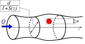
Figure 1: Schematic sketch of the flow carrying a spherical particle with radius $R$ within a tube of varying diameter. The total volumetric flow of the fluid is $Q$.

II Flow in wavy tube

The situation is shown schematically in Fig. 1. The coordinate axis $z$ coincides with the tube axis and the diameter of the tube is governed by the periodic function $S(z)$. As the geometry of the tube is axially symmetric, we can use the cylindrical coordinates and describe the flow by the (Stokes) stream function $\psi(\rho,z)$ satisfying a fourth-order partial differential equation (see Appendix A).

When the diameter of the tube depends on the coordinate $z$ along the axis, it is convenient to change further to the generalized cylindrical coordinates

$$\begin{split}&\tilde{\rho}=(1+S(z))\rho\\ &\tilde{z}=z\;.\end{split}$$ (1)

With such coordinates the tube wall is at fixed value $\tilde{\rho}=d/2$, which simplifies the treatment of boundary conditions. The function $S(z)$ describes variation of the diameter around its medium value $d$ and it is supposed to vary periodically along the tube. Therefore, we can expand it in terms of Fourier components

$$S(z)=\sum_{k=1,2,\ldots}\left(A_{k}\sin k\Omega z+B_{k}\cos k\Omega z\right)\;.$$ (2)

If $S=0$, inertial terms in the NS equations vanish. Therefore, our strategy will be to expand in powers of the Fourier amplitudes of $S(z)$. The stream function is then written as

$$\psi(\tilde{\rho},\tilde{z})=\psi_{0}(\tilde{\rho})+\psi_{1}(\tilde{\rho},\tilde{z})+\psi_{2}(\tilde{\rho},\tilde{z})+\ldots$$ (3)

where $\psi_{n}$ contains $n$-th powers of the amplitudes $A_{k}$, $B_{k}$. The lowest inertial corrections are contained in the term $\psi_{1}$.

The equation for $\psi$ is non-linear, but we can transform it into a chain of linear equations. Indeed, the equation for $\psi_{0}$ is linear and if we already know functions $\psi_{0}$ through $\psi_{n-1}$, we can insert them into an equation which is linear in the unknown $\psi_{n}$. Here we shall stop at the lowest correction $\psi_{1}$.

Finding the zeroth term $\psi_{0}$ is trivial as it does not depend on $\tilde{z}$. The solution satisfying the proper boundary conditions is

$$\psi_{0}(\tilde{\rho})=\frac{4Q}{\pi}\left(\frac{\tilde{\rho}}{d}\right)^{2}\left(1-2\left(\frac{\tilde{\rho}}{d}\right)^{2}\right)$$ (4)

and we can see that the formula is formally identical to the standard Poiseuille flow, but expressed in the variable $\tilde{\rho}$.

Knowing $\psi_{0}$, we can write a linear equation for $\psi_{1}$. In analogy to (2), we can expand it into sum of Fourier components

$$\psi_{1}(\tilde{\rho},\tilde{z})=\sum_{k=1,2,\ldots}\Big{(}\alpha_{k}(\tilde{\rho})\sin k\Omega\tilde{z}+\beta_{k}(\tilde{\rho})\cos k\Omega\tilde{z}\Big{)}\;.$$ (5)

The boundary conditions at the tube wall and at the axis require that

$$\begin{split}\alpha_{k}\Big{(}\frac{d}{2}\Big{)}=\alpha^{\prime}_{k}\Big{(}\frac{d}{2}\Big{)}=\beta_{k}\Big{(}\frac{d}{2}\Big{)}=\beta^{\prime}_{k}\Big{(}\frac{d}{2}\Big{)}=0\\ \alpha_{k}(0)=\alpha^{\prime}_{k}(0)=\beta_{k}(0)=\beta^{\prime}_{k}(0)=0\;.\end{split}$$ (6)

This has an important consequence that the volumetric flow through the tube resulting from $\psi_{1}$ is zero, so the total volumetric flow is always $Q$ as given by $\psi_{0}$. Of course, the quantity which is affected by non-zero $\psi_{1}$ is the pressure.

It turns out that the components with different index $k$ are independent. This greatly simplifies the solution which at the end can be written in a compact form as

$$\begin{split}\psi_{1}(\tilde{\rho},\tilde{z})=&-\frac{2Q}{\pi}\,\mathrm{Im}\sum_{k}\Big{[}g\Big{(}k\Omega\tilde{\rho};k\Omega\frac{d}{2},\frac{2k\Omega Q}{\pi\nu}\Big{)}\times\\ &\times(A_{k}-\mathrm{i}B_{k})\,\exp(-\mathrm{i}k\Omega\tilde{z})\Big{]}\;.\end{split}$$ (7)

The complex function $g(x;r,t)$ of variable $x$ depends on parameters $r$ and $t$ and can be found as a solution of the equation

$$(L_{2}-\mathrm{i}t\,L_{1})g(x;r,t)=-K_{2}+\mathrm{i}t\,K_{1}$$ (8)

where the operators $L_{1}$ and $L_{2}$ and functions $K_{1}$ and $K_{2}$ are

$$L_{1}=\Big{(}\frac{x}{r}\Big{)}^{2}\Big{[}1-\Big{(}\frac{x}{r}\Big{)}^{2}\Big{]}\Big{(}-x^{2}\frac{d^{2}}{dx^{2}}+x\frac{d}{dx}+x^{2}\Big{)}$$ (9)

$$\begin{split}L_{2}=&x^{4}\frac{d^{4}}{dx^{4}}-2x^{3}\frac{d^{3}}{dx^{3}}+\big{(}3x^{2}-2x^{4}\big{)}\frac{d^{2}}{dx^{2}}+\\ &+\big{(}-3x+2x^{3}\big{)}\frac{d}{dx}+x^{4}\end{split}$$ (10)

$$K_{1}=\frac{x^{6}}{r^{4}}\Big{[}\frac{8}{r^{2}}+1-\Big{(}\frac{8}{r^{2}}+2\Big{)}\Big{(}\frac{x}{r}\Big{)}^{2}+\Big{(}\frac{x}{r}\Big{)}^{4}\Big{]}$$ (11)

$$K_{2}=\frac{x^{6}}{r^{2}}\Big{[}\frac{16}{r^{2}}+1-\Big{(}\frac{x}{r}\Big{)}^{2}\Big{]}\;.$$ (12)

For certain specific values of $t$ it is possible to write the solution of (8) in terms of hypergeometric functions. In general case we expand the function $g(x;r,t)$ in powers of the parameter $t$ and solve separately the equations for the expansion coefficients. So, if $g(x;r,t)=\sum_{m=0}^{\infty}(\mathrm{i}t)^{m}\,g^{(m)}(x;r)$, we have the chain of equations for the components $g^{(m)}(x;r)$

$$\begin{split}L_{2}\,g^{(0)}&=-K_{2}\\ L_{2}\,g^{(1)}&=L_{1}\,g^{(0)}+K_{1}\\ L_{2}\,g^{(2)}&=L_{1}\,g^{(1)}\\ &\vdots\end{split}$$ (13)

which can be solved step by step in terms of Bessel functions. We defer explicit formulas for the solution to the Appendix B. Here we show only the series expansion in powers of $x$, where the coefficients are finite sums of powers of the fraction $\xi=(x/r)^{2}$

$$\begin{split}&g^{(1)}(x;r)=-\frac{\xi^{4}}{144}+\frac{\xi^{3}}{24}-\frac{\xi^{2}}{16}+\frac{\xi}{36}-\\ &-\Big{(}\frac{\xi^{4}}{2304}-\frac{5\,\xi^{3}}{1728}+\frac{\xi^{2}}{144}-\frac{\xi}{144}+\frac{17}{6912}\Big{)}x^{2}+\\ &+\ldots\end{split}$$ (14)

which will be useful later.

In fact, the expansion parameter $t$ is proportional to the tube Reynolds number multiplied by the quantity $k\Omega d$. Therefore, the expansion can be considered as small-Reynolds number expansion. However, this holds only as long as $k\Omega$ is not too large. If the spatial frequency of the tube modulation $\Omega$ is large and/or if the modulation is not smooth but exhibits sharp edges (i. e. large $k$ must be taken into account) the expansion is no more useful and full solution of (8) is necessary.

We shall use the following specific form of diameter modulation

$$S(z)=A\sin 2\Omega z+B\cos\Omega z$$ (15)

which is indeed fairly smooth. For small $\Omega d$ and small $\mathrm{Re}_{t}$, taking only lowest terms in the $t$-expansion is a sensible approximation. At this point it is perhaps appropriate to make a general remark concerning approximations made. As always in a hydrodynamics problem it is always a Reynolds number which decides on applicability of this or that approximation. In a complex geometry, there are always several Reynolds numbers, and in our work we already mentioned two of them, namely the tube and particle Reynolds numbers. However, also the value $2k\Omega Q/\pi\nu$ assigned to the expansion parameter $t$ can be regarded as a Reynolds number relating the flow velocity $U$ to two geometric parameters, the average tube diameter $d$ and the spatial period of the diameter variations $1/\Omega$. More precisely, there are several harmonic components, i. e. terms with $k=1,2,3,\ldots$, and each of them introduces its own length scale $1/k\Omega$. Therefore, there is a Reynolds number for each of the harmonic components. The small-$t$ expansion means that all these Reynolds numbers must be $\ll 1$. For our target value of the tube Reynolds number $\mathrm{Re}_{t}\simeq 2$ and supposing that the highest harmonic component has $k=2$, as in (15), this is satisfied as long as $\Omega d\ll 1$, i. e. the spatial period is much monger that the tube diameter. As a practical example, the experiments in mat_mul_gos_11 have $d\simeq 3\;\mu$m, $\Omega\simeq 10^{5}\;\mathrm{m}^{-1}$ $\mathrm{Re}_{t}\simeq 0.2$ and therefore satisfy the condition. However, if the flow were faster, e. g. $\mathrm{Re}_{t}\simeq 20$, the condition would be proportionally stronger, i. e. spatial period would have been much larger than ten times the diameter.

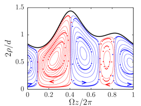
Figure 2: Streamlines of the difference flow according to (16) in a tube with profile given by (15) where $A=0.15$ and $B=0.2$. The orientation of the flow is indicated by arrows. The thick curve indicates the tube wall. Using heavy dots we plot also the results of exact solution using OpenFoam, with $\nu=10^{-6}\,\mathrm{m}^{2}\mathrm{s}^{-1}$ (water), $d=0.3\,\mathrm{mm}$, $U=5\,\mathrm{mms}^{-1}$. (This means $Q=0.245\ldots\,\mathrm{mm}^{3}\mathrm{s}^{-1}$, $\mathrm{Re}_{t}=1.5$.) Note that the vertices would be totally absent if the flow were described by Stokes equation.

Rectification of the colloid flow occurs when the fluid is pumped periodically back and forth by a piston. In such movement, the fluid as a whole returns back to its original position after each period. We shall consider the pumping adiabatic, composed of a first half-period of stationary flow in one direction and a second half-period of stationary flow in the opposite direction. The stream function in the first and second half-period differ only in the sign of the parameter $Q$. The difference flow is then simply the arithmetic average of the two. The stream function of the difference flow, denoted $\delta\psi$, then contains only even powers of $Q$. Therefore, it is obtained from (7) by replacing $g(x;r,t)$ by expansion containing only odd powers of $t$. If we keep only the lowest term, we get the difference stream function

$$\begin{split}\delta\psi&(\tilde{\rho},\tilde{z})=\frac{4\Omega Q^{2}}{\pi^{2}\nu}\,\sum_{k}\Big{[}k\,g^{(1)}\Big{(}k\Omega\tilde{\rho};\frac{1}{2}k\Omega d\Big{)}\times\\ &\times(B_{k}\sin k\Omega\tilde{z}-A_{k}\cos k\Omega\tilde{z})\Big{]}+O(\mathrm{Re}_{t}^{3})\;.\end{split}$$ (16)

We show in Fig. 2 streamlines of the flow described by (16) in the tube of profile (15). We can see alternating clockwise and counterclockwise vortexes, whose placing reflects the variations of the tube diameter. The spatial extent of each vortex along the tube approximately copies the segments of monotonous change of the diameter. Note that the existence of the vortexes is purely inertial effect. Any solution of the Stokes equation would give $\delta\psi$ identically zero.

To check the quality of the two approximations made (i. e. small $S$ and small $t$), we solved the Navier-Stokes equations numerically, using the package OpenFoam, for the parameters as shown in Fig. 2. If we compare the streamlines according to (16) with the exact result, we can see quite good agreement. The position and shape of the vortexes is reproduced well, the main difference being that the approximate streamlines according to (16) are more rounded. This indicates that higher harmonic components, i. e. higher powers of $S$ would be necessary for better agreement.

III Spherical particle in ambient flow

Now let us insert a spherical particle of radius $R$ into the flow. The particle is considered neutrally-buoyant. The perturbation to the ambient flow (7) due to the presence of the particle and thus the force acting on a spherical particle can be computed by standard methods lan_lif_87 ; kim_kar_05 , expanding the ambient flow into Taylor series around the center of the sphere. In our actual calculations we took the Taylor series up to quadratic terms only. Taking higher terms in this expansion would result in terms of higher order in $R$ in the formula for particle drift.

The perturbation is found by solving the Stokes equation, which is a valid approximation if the particle size is much smaller than the tube diameter, so that $\mathrm{Re}_{p}\ll 1$ even if $\mathrm{Re}_{t}\gtrsim 1$. The truncated Taylor expansion of the ambient flow serves as boundary condition at infinity. Certainly, this strategy fails when the distance from the surface of the particle to the wall is comparable with the particle diameter itself. In such case the hydrodynamic interactions are crucial and must be treated separately. However, when $d\gg R$, as we suppose throughout, the probability of particle being so close to the wall is very small. Therefore, we neglect this effect here.

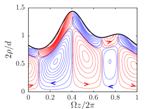
Figure 3: Streamlines of the difference flow of particles, according to formula (18), in a tube with identical parameters as in Fig. 2.

The result valid for an axisymmetric flow is the following. If the ambient flow is described by the stream function $\psi$, there is also a stream function

$$\psi_{\mathrm{p}}=\psi+\frac{R^{2}}{6}\Big{(}\frac{\partial^{2}}{\partial z^{2}}+\frac{\partial^{2}}{\partial\rho^{2}}-\frac{1}{\rho}\frac{\partial}{\partial\rho}\Big{)}\psi+O\big{(}R^{4}\big{)}$$ (17)

which corresponds to the velocity field of the particle drift. We shall neglect terms of higher order in the particle radius. In fact, they are also of higher order in the particle Reynolds number. Thus we arrive at nothing else than the Faxén law, which would be exact if the ambient flow was a solution of Stokes, rather than Navier-Stokes equation kim_kar_05 .

When the fluid is pumped back and forth, we can establish the difference flow of the particles, in analogy with the difference flow of the fluid. Denote $\delta\psi_{\mathrm{p}1}$ the stream function for the difference flow of particles to the first order in $t$. To this order we obtain

$$\begin{split}\delta\psi_{\mathrm{p}1}(\tilde{\rho},\tilde{z})=&\frac{4\Omega^{3}Q^{2}}{\pi^{2}\nu}\,\sum_{k}\Big{[}k^{3}\Big{(}g^{(1)\prime\prime}\big{(}k\Omega\tilde{\rho};\frac{k\Omega d}{2}\big{)}-\\ -\frac{1}{k\Omega\tilde{\rho}}\,g^{(1)\prime}&\big{(}k\Omega\tilde{\rho};\frac{k\Omega d}{2}\big{)}-g^{(1)}\big{(}k\Omega\tilde{\rho};\frac{k\Omega d}{2}\big{)}\Big{)}\times\\ &\times(B_{k}\sin k\Omega\tilde{z}-A_{k}\cos k\Omega\tilde{z})\Big{]}\end{split}$$ (18)

where prime means differentiation with respect to the variable $x$. The streamlines corresponding to particle drift according to (18) are plotted in Fig. 3. We can see marked difference from the fluid streamlines shown in Fig. 2. There are vortexes as in Fig. 2, but near the walls there are also “half-vortexes” which imply that at some places the drift pushes the particles towards the wall while at other places the particles are pulled away. To understand this effect properly, we must keep in mind that the difference flow depicts what happens after a whole period of pumping is completed. During the period the particle can follow some trajectory which may be complicated, but at the end of the period the particle is found shifted along the streamlines of Fig. 3 from its initial position. The pushing and pulling is therefore a summary effect of the movement over the whole period. Again, we should stress that the non-zero difference flow (18) is purely inertial effect and would be exactly zero if the ambient flow were described by Stokes equation. Finally, let us note that the hydrodynamic interaction of the particle with the wall, which is not considered here, would lead to modification of the half-vertexes on the scale $\simeq R$ from the wall. As $R\ll d$, we neglect it here.

The presence of “half-vortexes” also means that the particle drift, when integrated over the cross-section of the tube, depends on the coordinate $z$. This suggests an approximate mapping of the particle drift on an effective one-dimensional movement. The drift velocity imposed on the particle in such mapping is simply, according to the general properties of the stream function, $w(z)=8\big{(}\delta\psi_{\mathrm{p}1}(d/2,z)-\delta\psi_{\mathrm{p}1}(0,z)\big{)}/d^{2}$. For the specific profile (15) we get

$$\begin{split}w(z)=\frac{16\,Q^{2}R^{2}\Omega^{3}}{3\pi^{2}d^{2}\nu}\Big{[}&g^{(1)\prime\prime}\big{(}\frac{1}{2}\Omega d;\frac{1}{2}\Omega d\big{)}B\sin\Omega z-\\ -8\,&g^{(1)\prime\prime}\big{(}\Omega d;\Omega d\big{)}A\cos 2\Omega z\Big{]}\;.\end{split}$$ (19)

IV Ratchet effect

The drift (19) is a periodic function of $z$ and therefore does not impose any ratchet current by itself. To see the rectification of the particle flow, hydrodynamics must be accompanied by diffusion. The full analysis of the hydrodynamic ratchet would require solving the three-dimensional axially symmetric diffusion problem in the tube with spatially dependent drift given by (18). However, here we remain on a simpler level and estimate the ratchet effect by mapping on a one-dimensional diffusion problem. In fact, we already started this program by computing the effective drift (19). Using the standard Fick-Jacobs mapping zwanzig_92 ; reg_sch_bur_rub_rei_han_06 , we have, to first order in $S(z)$, the stationary diffusion equation

$$0=\frac{\partial}{\partial z}\Big{[}(-w(z)\pm h+2DS^{\prime}(z))\,P(z)\Big{]}+D\frac{\partial^{2}}{\partial z^{2}}P(z)\;.$$ (20)

The diffusion coefficient for a sphere is $D=kT/(6\pi\rho_{f}\nu R)$, where $\rho_{f}$ is here the density if the fluid. The term $h$ accounts for steady driving due to the periodic pumping. Its amplitude is $h=4Q/(\pi d^{2})$ and the sign is positive in one half-period and negative in the other one. In fact, this term stands for all terms with even power of $Q$ in the expansion of the ambient flow. As the leading term of this type is independent of $z$, we can safely approximate it by constant $h$. The equation (20) describes a standard Brownian motor which is exactly solved in the literature reimann_02 .

The advection term contains the hydrodynamic drift $w(z)$ and the term $DS^{\prime}(z)$ describing the entropic barrier. Using the average velocity $U=4Q/\pi d^{2}$, the condition for the former to dominate the latter can be written as

$$\frac{2}{3}U^{2}R^{3}\,\rho_{f}\gg kT\;.$$ (21)

Considering neutrally-buoyant colloidal particle, this condition can be understood so that the kinetic energy of the particle as carried by the fluid is much larger that the thermal quantum $kT$. For parameters used in Fig. 2 and at normal laboratory temperature the condition (21) is satisfied for particles larger than about $0.5\mu\mathrm{m}$. Therefore, the typical particles used in experiments like mat_mul_03 or all kinds of blood cells satisfy (21).

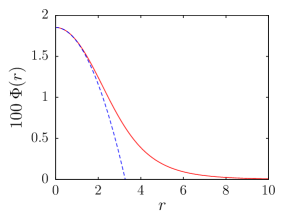
Figure 4: Graph of the function $\Phi(r)$ defined by (23). The approximation (24) is drawn by the dashed line

The exact solution of the motor described by (20), as shown in reimann_02 , is given by a complicated formula. If we are in the hydrodynamic regime (21), and if we expand the solution in powers of $A/kT$ and $B/kT$, and simultaneously in the quantity $Q/(d^{2}\Omega kT)$, we obtain for the average ratchet velocity of the particle

$$\langle v_{\mathrm{p}}\rangle=\frac{2}{9}\Big{(}\frac{6\pi\rho_{f}}{kT}\Big{)}^{4}\frac{\nu}{\Omega}\Big{(}\frac{4Q}{\pi d^{2}}\Big{)}^{8}\,R^{10}\,\Phi(\Omega d)\,A^{2}B$$ (22)

where

$$\Phi(r)=r^{6}\big{(}g^{(1)\prime\prime}(r;r)\big{)}^{2}\,g^{(1)\prime\prime}(r/2;r/2)\;.$$ (23)

For tubes narrow with respect to the spatial period of the diameter modulation we can use (14) and expand the function $\Phi(r)$ in powers

$$\Phi(r)=\frac{1}{54}-\frac{r^{2}}{576}+O(r^{4})\;.$$ (24)

In the opposite limit $r\to\infty$ the function $\Phi(r)$ decreases to zero, reflecting the fact that the ratchet effect vanishes if the diameter changes too fast along the tube. The full form of the function $\Phi(r)$ is shown in Fig. 4, together with the approximation (24), which is good as long as $r\lesssim 2$. In practice this condition just tells us that the spatial period of tube modulation must be at least half of the tube diameter.

We can see that the dependence of the ratchet current on the particle diameter is extremely strong, much stronger than what would be seen with entropic barriers only. This can be traced to the diameter dependence of the hydrodynamic drift (19). We believe here is a potential for practicable particle sorting. In this direction, it is essential to choose the tube variation in an optimal way. Unfortunately, there is no obvious way how to prescribe the optimal shape, as is the case already with the simplest Brownian ratchet solved in reimann_02 . For optimization purposes the limits of small amplitudes $A$ and $B$ used when deriving Eq. (22) are not sufficient and numerical evaluation of the exact formula (Equations (5.2-3) in reimann_02 ) is unavoidable. Some statements can be made, though. In our case, the effective ratchet potential has its origin in the half-vortexes, as exemplified in Fig. 3. These half-vortexes stem from the second derivative of the ambient flow and therefore it seems plausible to suppose that they are more pronounced if the second derivative of the ambient flow is higher. This may happen if the flow is less “smooth”, e. g. for tubes with sharp edges. However, this is just a hypothesis which would require thorough testing.

V Conclusions

To conclude, we provided an analytic solution of the problem of a spherical colloidal particle carried by a fluid flow in a tube of variable diameter. The primary approximation is taking only lowest term in the expansion in powers of the amplitude of diameter modulation. The solution is approximate but agrees well with direct numerical solution of NS equations in the regime of Reynolds number we used, $\mathrm{Re}_{t}\simeq 1.5$. Further improvement is possible taking into account higher powers of the amplitude, but mixing together various harmonic modes would make the analysis rather complicated.

The fluid is pumped back and forth so that the average fluid flow is zero. Inertial effects are non-negligible and lead to non-trivial drift acting on the particle. Attention should be paid on the inertial effects when interpreting the experimental results, as the regime in which the flow oscillates with no average volumetric bias is not the same as regime in which the pressure oscillates symmetrically with no pressure bias. With tube profile breaking the mirror symmetry the inertial effects make the two regimes different.

Combining the inertial hydrodynamic particle drift with diffusion, a ratchet effect occurs, rectifying the average movement of the particle. We analyzed it by standard mapping on a one-dimensional problem. We found a criterion when this inertial hydrodynamic effect dominates the effect of entropic barriers (which is nevertheless always present). We showed that the average ratchet velocity depends very strongly on the particle radius. The dependence is much more pronounced than with entropic barriers. Therefore, inertial hydrodynamics opens a promising perspective for new approach in sorting particles according to their size, which may be more efficient than sorting with entropic barriers only. Detailed comparison of the two regimes, as well as the study of the crossover between the two, which must occur when the fluid velocity is gradually increased, would deserve special study, which we leave for future.

Another interesting ramification of this hydrodynamic study concerns the situation in which Brownian particles in asymmetric channels are driven by electrostatic or gravitational force. The interplay between these external forces and hydrodynamics was already studied mar_sch_str_sch_han_13 ; mar_str_sch_sch_han_13 , but as far as we know inertial effects were left aside. But as a matter of fact driven particles immersed in the fluid induce flows in the otherwise resting fluid and these flows can have components which go beyond the Stokes approximation. Existence of such inertial effects was demonstrated in sedimentation experiments, e. g. in che_mcl_90 , but their relevance for electrostatically driven transport in micropores remains to be studied.

A natural question arises what are the limits of applicability of the current analytic approximation. We checked, as also shown in Fig. 2, that the approximation gives good results when compared to exact numerical solution of NS equations for tube Reynolds numbers up to about $\mathrm{Re}_{t}\simeq 1.5$. For example in mat_mul_gos_11 the data suggest Reynolds numbers up to $\mathrm{Re}_{t}\simeq 0.7$, so the present theory should be well appropriate to describe their experiments. We believe that our theory is in principle applicable to even higher Reynolds numbers. Currently we do not have a systematic data available, but we can estimate the limits from other works using the same level of approximation in the study of Segré-Silberberg effect. For example in asmolov_02 it is claimed that their approximation remains valid up to Reynolds numbers in the range of several hundreds. We hypothesize that our approximation may be restricted by similar limits. In practice it means that e.g. the experiments with sorting polystyrene spheres by Segré-Silberberg effect bha_kun_pap_08 , where the Reynolds number achieved was $\mathrm{Re}_{t}\simeq 40$, fall probably within the validity of the present theory. Also the experiment with tumor cell separation in sun_liu_li_wan_xia_hu_jia_13 used Reynolds numbers at most $100$, hence we believe our method would be applicable too. On the other hand, in another tumor-cell sorting experiment reported in mac_kim_ars_hur_dic_11 , the Reynolds number was much higher, $\mathrm{Re}_{t}\simeq 1500$. It would require a separate study to see, whether our theory is still valid for such rapid flows.

Finally, we believe that the method used in this work can be adapted to broader range of problems in quasi-one-dimensional transport. For example, there is growing interest in the dynamics of active particles in confined geometries bec_dil_low_rei_vol_vol_16 . Separation of such particles is an interesting problem ber_etal_13 and our method could be perhaps adapted by simply replacing Eq. (17) by stream function appropriate to active particles. Investigations in this direction are in course.

Another modification can be inspired by the recent work ver_par_pos_15 where angular velocity component is forced onto granular flow by spiral structures, not unlike rifling of gun barrels. If such rifling were possible in a microfluidic channel, it could also be used to induce inertial ratchet effect. In this case, the system is still axially symmetric, if we consider the rifling infinitesimally fine. Therefore our method is still applicable in principle, but must be generalized by allowing non-zero angular velocity in the flow. On the better side, in such setup we could avoid the (rather big) technical complications arising from the use of generalized cylindrical coordinates. Other kinds of curved and spiraling shapes of the tubes are also conceivable, but as soon as we loose the axial symmetry, analytical approaches become too difficult.

Appendix A Stokes stream function

An axisymmetric flow with zero azimuthal component can be expressed in terms of the Stokes stream function $\psi(\rho,z)$, related to the cylindrical components of the velocity field as

$$\begin{split}u_{\rho}=-\frac{1}{\rho}\frac{\partial\psi}{\partial z}\\ u_{z}=\frac{1}{\rho}\frac{\partial\psi}{\partial\rho}\;.\\ \;\end{split}$$ (25)

Then, the continuity equation is satisfied automatically and the Navier-Stokes equation translates in the fourth-order equation for $\psi(\rho,z)$, which can be written as

$$\begin{split}\frac{1}{\rho^{2}}\left(\frac{\partial\psi}{\partial z}\frac{\partial}{\partial\rho}-\frac{\partial\psi}{\partial\rho}\frac{\partial}{\partial z}\right)\left(\frac{\partial^{2}\psi}{\partial\rho^{2}}+\frac{\partial^{2}\psi}{\partial z^{2}}\right)+\frac{1}{\rho^{3}}\left(\frac{\partial\psi}{\partial\rho}\frac{\partial^{2}\psi}{\partial\rho\partial z}-3\frac{\partial\psi}{\partial z}\frac{\partial^{2}\psi}{\partial\rho^{2}}-2\frac{\partial\psi}{\partial z}\frac{\partial^{2}\psi}{\partial z^{2}}\right)+3\frac{1}{\rho^{4}}\frac{\partial\psi}{\partial\rho}\frac{\partial\psi}{\partial z}=\\ -\nu\left\{\frac{1}{\rho}\left(\frac{\partial^{4}\psi}{\partial\rho^{4}}+2\frac{\partial^{4}\psi}{\partial\rho^{2}\partial z^{2}}+\frac{\partial^{4}\psi}{\partial z^{4}}\right)-2\frac{1}{\rho^{2}}\frac{\partial}{\partial\rho}\left(\frac{\partial^{2}\psi}{\partial\rho^{2}}+\frac{\partial^{2}\psi}{\partial z^{2}}\right)+3\frac{1}{\rho^{3}}\frac{\partial^{2}\psi}{\partial\rho^{2}}-3\frac{1}{\rho^{4}}\frac{\partial\psi}{\partial\rho}\right\}\;.\end{split}$$ (26)

The next step is writing the equation in terms of the generalized cylindrical coordinates (1). The derivatives transform as

$$\begin{split}&\frac{\partial}{\partial{\rho}}=\big{(}1+S(\tilde{z})\big{)}\,\frac{\partial}{\partial\tilde{\rho}}\\ &\frac{\partial}{\partial{z}}=\frac{\partial}{\partial\tilde{z}}+\frac{S^{\prime}(\tilde{z})}{1+S(\tilde{z})}\,\tilde{\rho}\,\frac{\partial}{\partial\tilde{\rho}}\end{split}$$ (27)

and inserting them into (26) we obtain the desired equation for the stream function. When we neglect in this equation all terms of higher order than linear in the modulation amplitude, we finally arrive at equations for $\psi_{0}(\tilde{\rho})$ and $\psi_{1}(\tilde{\rho},\tilde{z})$.

Appendix B Explicit formulas for expansion in powers of $t$

The solution of the equation

$$(L_{2}-\mathrm{i}t\,L_{1})g(x;r,t)=-K_{2}+\mathrm{i}t\,K_{1}$$ (28)

is expanded as $g(x;r,t)=\sum_{m=0}^{\infty}(\mathrm{i}t)^{m}\,g^{(m)}(x;r)$. To establish the expansion coefficients $g^{(m)}$ we have to solve the chain of equations (13). Generally, the real functions $g^{(m)}$ can be written in terms of a particular solution and a combination of independent solutions of the homogeneous equation $L_{2}\phi(x)=0$. As two independent solutions of the homogeneous equation, satisfying the proper boundary conditions, we choose the functions

$$H_{1}(x)=xI_{1}(x)$$ (29)

$$\begin{split}&H_{2}(x)=\\ &x^{2}K_{1}(x)\Big{(}xI_{0}^{2}(x)-xI_{1}^{2}(x)-2I_{0}(x)I_{1}(x)\Big{)}+\\ &+2xI_{1}(x)\int_{0}^{x}x^{\prime}K_{1}(x^{\prime})I_{1}(x^{\prime})\,dx^{\prime}\;.\\ \;\end{split}$$ (30)

The other two linearly independent solutions do not satisfy the boundary conditions at the axis of the tube and would be taken into account only if the tube contained a concentric hard core.

Then, the $m$-th term can be written as a linear combination of the functions $H_{1}$ and $H_{2}$ plus the particular solution, i. e.

$$\begin{split}g^{(m)}(x;r)=\,&h_{1}^{(m)}(r)\,H_{1}(x)+h_{2}^{(m)}(r)\,H_{2}(x)+\\ &+P^{(m)}(x;r)\;.\end{split}$$ (31)

We show here explicitly the results for $m=0$ and $m=1$. In the zeroth order, the particular solution is

$$P^{(0)}(x;r)=\Big{(}\frac{x}{r}\Big{)}^{4}-\Big{(}\frac{x}{r}\Big{)}^{2}$$ (32)

and the coefficients in the linear combination are

$$h_{1}^{(0)}(r)=-2\Big{(}K_{1}(r)+2I_{1}(r)\,\phi_{2}(r)\Big{)}\,\phi_{3}(r)$$ (33)

$$\begin{split}h_{2}^{(0)}(r)=2I_{1}(r)\,\phi_{1}(r)\,\phi_{3}(r)\end{split}$$ (34)

where we defined auxiliary functions

$$\phi_{1}(r)=\frac{1}{r^{2}I_{0}^{2}(r)-r^{2}I_{1}^{2}(r)-2rI_{0}(r)I_{1}(r)}$$ (35)

$$\phi_{2}(r)=\phi_{1}(r)\int_{0}^{r}x^{\prime}K_{1}(x^{\prime})I_{1}(x^{\prime})\,dx^{\prime}$$ (36)

and

$$\phi_{3}(r)=\frac{1}{r^{2}\Big{(}K_{1}(r)I_{0}(r)+I_{1}(r)K_{0}(r)\Big{)}}\;.$$ (37)

In the first order, the particular solution can be written as

$$\begin{split}&P^{(1)}(x;r)=\\ &2x\,\Big{(}I_{1}(x)f_{1}(x;r)-K_{1}(x)f_{2}(x;r)\Big{)}\,h_{2}^{(0)}(r)\\ \;\end{split}$$ (38)

and the coefficients as

$$h_{1}^{(1)}(r)=-2\Big{(}f_{1}(r;r)+2\,f_{2}(r;r)\,\phi_{2}(r)\Big{)}h_{2}^{(0)}(r)$$ (39)

$$h_{2}^{(1)}(r)=2f_{2}(r;r)\,\phi_{1}(r)\,h_{2}^{(0)}(r)$$ (40)

where

$$\begin{split}f_{1}(x;r)=\int_{0}^{x}\int_{0}^{x^{\prime}}x^{\prime}K_{1}(x^{\prime})\Big{(}I_{1}(x^{\prime})K_{1}(y)-\\ -K_{1}(x^{\prime})I_{1}(y)\Big{)}f_{3}(y;r)\,dy\,dx^{\prime}\end{split}$$ (41)

$$\begin{split}f_{2}(x;r)=\int_{0}^{x}\int_{0}^{x^{\prime}}x^{\prime}I_{1}(x^{\prime})\Big{(}I_{1}(x^{\prime})K_{1}(y)-\\ -K_{1}(x^{\prime})I_{1}(y)\Big{)}f_{3}(y;r)\,dy\,dx^{\prime}\end{split}$$ (42)

and

$$\begin{split}&f_{3}(y;r)=\Big{[}\Big{(}\frac{y}{r}\Big{)}^{4}-\Big{(}\frac{y}{r}\Big{)}^{2}\Big{]}\times\\ &\times I_{1}(y)\Big{(}K_{1}(y)I_{0}(y)+I_{1}(y)K_{0}(x)\Big{)}\;.\end{split}$$ (43)