Quantum versus classical dynamics in the optical centrifuge

Abstract

The interplay between classical and quantum mechanical evolution in the optical centrifuge (OC) is discussed. The analysis is based on the quantum mechanical formalism starting from either the ground state or a thermal ensemble. Two resonant mechanisms are identified, i.e. the classical autoresonance and the quantum mechanical ladder-climbing, yielding different dynamics and rotational excitation efficiencies. The rotating wave approximation is used to analyze the two resonant regimes in the associated dimensionless two-parameter space and calculate the OC excitation efficiency. The results show good agreement between numerical simulations and theory and are relevant to existing experimental setups.

I Introduction

The rigid rotor is frequently used for studying the interplay between classical and quantum mechanical phenomena, as it is complex enough to offer intricate behavior and yet simple enough to be conveniently handled in both theories. For example, the periodically kicked rigid rotor problem classically may yield chaotic dynamics CKR1 ; CKR2 ; CKR3 , but quantum mechanically it is replaced by Anderson localization QKR1 ; QKR2 ; QKR3 . The optical centrifuge (OC) is another example of exploration of rotational dynamics on the molecular level. Originally proposed and implemented by Corkum and collaborators Corkum1 ; Corkum2 , instead of a periodic drive it uses a chirped frequency laser drive targeting the rotational degree of freedom of (mainly) diatomic molecules. Over the last few years, several state-of-the-art experiments Mullin ; Milner1 explored the OC dynamics, demonstrating ultrafast rotation and molecular dissociation Corkum2 , alteration of collisional decoherence Milner2 , rotational confinement Milner3 and even ultrafast magnetization Milner4 . The experiments use both hot gas of light molecules, and cold gas of heavy molecules, so one could expect to observe both quantum mechanical and classical responses.

In recent years, it was demonstrated that resonant chirped frequency drives are very useful in studying quantum and classical phenomena in various driven oscillatory systems, allowing exploration of the problem’s phase space. Depending on the characteristics of the system and the drive, the evolution in these driven systems takes a classical, quantum mechanical, or mixed form. In the classical limit, a persistent nonlinear phase locking between the driver and the system, known as autoresonance (AR) AR , allows for continued excitation. In contrast, in the quantum limit, the system undergoes successive Landau-Zener (LZ) transitions Landau ; Zener , or quantum ladder climbing (LC). Both regimes of operation were demonstrated and used in atoms and molecules LC1 ; LC1a ; LC1b ; LC2 ; AR1 , anharmonic oscillators AR , Josephson junctions LC3 , plasma waves PW1 ; PW2 , and cold neutrons Nu1 . An interesting and surprising effect in some driven chirped anharmonic oscillators is the forced dynamical transition from the quantum to the classical regime LC5 .

The optical centrifuge in its classical regime is an example of AR OurPaper . But how the transition from the classical AR in this driven system to quantum mechanical LC occurs? Of key importance in the OC is its efficiency, i.e. the fraction of molecules excited rotationally by the chirped laser drive. This issue was addressed recently in the AR regime of operation OurPaper . The corresponding quantum mechanical process was only studied numerically OCtheory1 or under the constraint $l=m$ OCtheory2 ; OCtheory3 , where $l,m$ are the quantum numbers associated with the total angular momentum and its projection on the laser propagation direction, respectively. The former assumption makes it impossible to study the response of a randomly oriented molecular ensemble to the OC pulse. The interplay between classical and quantum mechanical effects under different initial conditions in the system has not been studied to date. In this work, we use the quantum mechanical description of the OC in the rigid rotor approximation and show how it could give rise to the two different resonant mechanisms, the AR and LC. We will find criteria separating the two regimes in the parameter space, and calculate the corresponding OC efficiencies. We will use numerical simulations and theory for two sets of initial conditions, i.e. a fully populated ground-state and a ”hot” thermal ensemble and show that different combinations of parameters and initial conditions exhibit significantly different dynamics and efficiencies.

The scope of the paper will be as follows. In Sec. II, we introduce the model and the governing equations. Section III analyzes different resonant regimes using the rotating wave approximation and discusses typical excitation conditions in the associated parameter space. In the same section, the OC efficiency under various conditions is analyzed numerically and analytically for the aforementioned initial states. The section ends with a discussion of the relevance of our analysis to existing experiments. Our conclusions are summarized in Sec. IV.

II The model and parameterization

The OC uses a combination of two counter rotating and anti-chirped circularly polarized laser beams. The resulting field has acceleratingly rotating linear polarization, which can rotationally excite anisotropic molecules Corkum1 . Classically, this excitation process is an example of rotational autoresonance OurPaper , as the molecule continuously self-adjusts its rotation frequency to that of the accelerating rotation of drive. For a driving wave propagating along the $Z$ axis, with polarization angle $\phi_{d}\left(t\right)$ in the $XY$ plane, after averaging over the optical frequency of the laser beams, the interaction potential energy of a diatomic molecule in spherical coordinates is given by $U=-\varepsilon\sin^{2}\theta\cos^{2}\left(\varphi-\phi_{d}\right)$ Corkum1 , where $\varepsilon=\left(\alpha_{\parallel}-\alpha_{\perp}\right)E_{0}^{2}/4$, $\alpha_{\parallel}$,$\alpha_{\perp}$ are the polarizability components of the molecule and $E_{0}$ is the electric field amplitude of the combined laser beam. Similarly to existing experimental systems Milner1 ; Milner2 ; Milner3 , we will use a drive with zero initial frequency and linear frequency chirp $\omega_{d}=d\phi_{d}/dt=\beta t/2$, where $\beta>0$ is the chirp rate.

We will analyze the OC dynamics governed by the full quantum mechanical Hamiltonian $\widehat{H}=\widehat{H}_{0}+\widehat{U}$, using the set of eigenstates of the unperturbed Hamiltonian $\hat{H_{0}}=\hat{L}^{2}/2I$, where $\hat{L}$ is the angular momentum operator, and $I$ is the molecule’s moment of inertia. This set comprises the spherical harmonics $\left|l,m\right\rangle$, satisfying $\hat{L}^{2}\left|l,m\right\rangle=\hbar^{2}l\left(l+1\right)\left|l,m\right\rangle$, $\hat{L_{z}}\left|l,m\right\rangle=\hbar m\left|l,m\right\rangle$, where $\hat{L_{z}}$ is the operator associated with the projection of angular momentum on the $Z$ axis Sakurai . At this stage, we can identify three relevant time scales, i.e. the drive sweeping time $t_{s}=1/\sqrt{\beta}$, the Rabi (driving) time scale $t_{d}=\hbar/\varepsilon$ and the characteristic quantum mechanical ”rotation” time $t_{c}=I/\hbar$. The three time scales yield two dimensionless parameters:

$$P_{1}=\frac{t_{s}}{t_{d}}=\frac{\varepsilon}{\hbar\sqrt{\beta}},$$ (1)

and

$$P_{2}=\frac{t_{s}}{t_{c}}=\frac{\hbar}{I\sqrt{\beta}},$$ (2)

characterizing the driver’s strength and the problem’s nonlinearity, respectively. This parameterization yields the classical parametrization OurPaper , if one replaces the quantum mechanical action scale $\hbar$ by the action scale $\sqrt{Ik_{B}T}$ of a thermal classical ensemble, where $k_{B}$ is the Boltzmann constant and $T$ is the temperature.

The form of the interaction $\hat{U}$ leads to selection rules, where transitions are allowed to states with $\Delta l,\Delta m$ equal to $0$ or $\pm 2$ only. This also follows from the two-photon nature of these Raman processes and guarantees the conservation of parity for both $l,m$. Expressing the wave function in the Schrodinger equation for the driven problem as $\sum_{l,m}a_{l,m}\left|l,m\right\rangle$, the dimensionless evolution equation for coefficient $a_{l,m}$ in terms of parameters $P_{1,2}$ is given by:

$$i\frac{da_{l,m}}{d\tau}=E_{l}a_{l,m}+P_{1}\sum_{\begin{subarray}{c}\Delta l=\\ 0,\pm 2\end{subarray}}\sum_{\begin{subarray}{c}\Delta m=\\ 0,\pm 2\end{subarray}}c_{l,m}^{\Delta l,\Delta m}a_{l^{\prime},m^{\prime}}e^{i\Delta m\phi_{d}},$$ (3)

where the time derivative is with respect to the slow dimensionless time $\tau=\sqrt{\beta}t$, $l^{\prime}=l+\Delta l$, $m^{\prime}=m+\Delta m$ and $E_{l}={P_{2}}l\left(l+1\right)/2$. The details of the derivation, and the the coupling coefficients $c_{l,m}^{\Delta l,\Delta m}$ are given in Appendix A.

The evolution described by Eq. (3) exhibits different dynamics depending on parameters $P_{1,2}$ and initial condition. In this paper, we focus on two types of initial conditions, i.e. a fully populated ground state ($l=0$) and a finite temperature thermal state. For the purpose of this work, it is convenient to define the temperature via the characteristic $l$ value, $l_{c}\geq 0$, given by equating the thermal and rotational energies:

$$k_{B}T=\frac{\hbar^{2}}{2I}l_{c}\left(l_{c}+1\right).$$ (4)

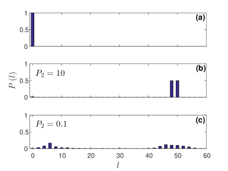
Figure 1: The normalized distribution of the $l$-states from the numerical solution of Eq. (3) for the ground state initial condition shown in panel (a). The resulting final distributions for $P_{2}=10$ are shown in panel (b) and for $P_{2}=0.1$ in panel (c). The parameter $P_{1}=10$ in both panels (b) and (c) and the final time is $\tau=99P_{2}$ .

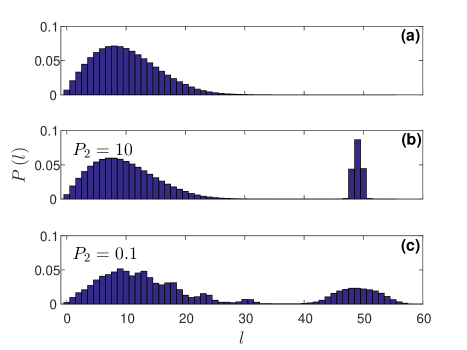
Figure 2: The normalized distribution of the $l$-states from the numerical solution of Eq. (3) for a thermal initial condition with $l_{c}=11.5$ (a). The resulting final distributions for $P_{2}=10$ are shown in panel (b) and for $P_{2}=0.1$ in panel (c). The parameter $P_{1}=10$ in both panels (b) and (c) and the final time is $\tau=99P_{2}$.

Figures 1 and 2 present numerical solutions of Eq. (3) starting from the ground state ($l=0$) (Fig. 1) and a thermal ensemble with $l_{c}=11.5$ (Fig. 2). These initial conditions ($\tau=0$) are shown on the top panels (a) in the figures, while the other panels show the final state at $\tau=99P_{2}$ for $P_{1}=10$. The values of $P_{2}$ were $10$ (panel b) and $0.1$ (panel c). The final driving frequency matches the resonant transition $l=48\rightarrow l=50$ (as will be explained below) and the resonantly excited population around this target state illustrates the results of different dynamics. Indeed, due to the conservation of parity of both $l,m$ when starting in the ground state, only even $l$ levels are excited, in contrast to the thermal ensemble where both even and odd excited states are present. Furthermore, for both initial conditions, the width of the population around the target state decreases dramatically with $P_{2}$. Finally, the fraction of excited population around the target state ranges from as high as $\sim 100\%$ (Fig. 1b) to as low as $\sim 17\%$ (Fig. 2b). We proceed to studying these characteristic evolutions next.

III Rotational LC versus classical AR

III.1 Resonant Evolution

In studying the different responses of the system to the chirped frequency drive, we examine the resonant interactions, which give rise to both the quantum mechanical LC and classical AR. The interaction $\hat{U}$ yields the coupling of each state $\left|l,m\right\rangle$ to itself and, in general, $8$ other states. However, not all of these transitions are resonant, and, to proceed, we apply the rotating wave approximation (RWA), the validity of which will be discussed below. We identify the nearest resonant transition $\left|l,m\right\rangle\rightarrow\left|l+2,m+2\right\rangle$ and apply the RWA, neglecting all nonresonant terms. This resonant transition conserves the difference $C=l-m$ and, therefore, the $m$ index is omitted in the following equations describing a given $C$ value. By transforming Eq. (3) to the rotating frame of reference, i.e defining $W_{l,m}=e^{il\phi_{d}}a_{l,m}$, and neglecting all nonresonant (rapidly oscillating) driving terms we get

$$i\dot{W_{l}}=\Gamma_{l}W_{l}+P_{1}c_{l}^{2}W_{l+2}+P_{1}c_{l}^{-2}W_{l-2},$$ (5)

where $\Gamma_{l}=E_{l}+P_{1}c_{l}^{0}-l\tau/2$. The coefficient $c_{l}^{0}$, which represents some energy shift, does not vary significantly between the coupled states, and its contribution in $\Gamma$ can usually be ignored. Then, the coupling matrix of a single Landau-Zener type Landau ; Zener two-level transition $l-2\rightarrow l$ is

$$\left(\begin{array}[]{cc}\frac{P_{2}}{2}\left(l-2\right)\left(l-1\right)-\frac{\tau}{2}\left(l-2\right)&P_{1}B_{l}\\ P_{1}B_{l}&\frac{P_{2}}{2}l\left(l+1\right)-\frac{\tau l}{2}\end{array}\right),$$ (6)

where $B_{l,m}=c_{l-2,m-2}^{2,2}=c_{l,m}^{-2,-2}$ and again index $m$ is omitted. Following the reasoning of Ref. LC2 ; LC5 , for having successive Landau-Zener (LZ) transitions in our chirped system, the duration of each transition must be much shorter than the time between two successive transitions. The time $\tau_{l}$ of each transition is given by the energy crossing condition, or $\Delta\Gamma=\Gamma_{l}-\Gamma_{l-2}=0$, yielding $\tau_{l}=P_{2}\left(2l-1\right)$, so the time between successive transitions is $4P_{2}$. The duration of a transition is $O\left(1\right)$ when $\left|B_{l}P_{1}\right|$ is small and $O\left(\left|B_{l}P_{1}\right|\right)$ when it is large LC5 . Therefore, we estimate the duration of the transition as $1+\left|B_{l}P_{1}\right|$. Consequently, the condition for the successive LC process is:

$$P_{2}\gg\frac{1}{4}+\frac{P_{1}}{16},$$ (7)

where we took $\left|B_{l}\right|$ at its maximal value of $1/4$ for all $C$ (see Appendix A).

When condition (7) is met, the transitions are well separated, only two states are coupled at a time, and LC takes place. When transitioning to an unpopulated state, The transition probability in a single LZ step is given by Landau ; Zener :

$$P_{l-2\rightarrow l}=1-\exp[-2\pi(P_{1}B_{l})^{2}].$$ (8)

The efficiency of this process is governed by $P_{1}$ only, and when its value is sufficiently large the transitions could yield nearly $100\%$ population transfer. If the OC proceeds from the ground state and the chirped driving frequency passes the resonance with some higher state $\widehat{l}$, the fraction of rotationally excited population with $l\geq\widehat{l}$ will be

$$f(\widehat{l})=\prod_{n=1}^{\widehat{l}/2}\left\{1-\exp\left[-2\pi(P_{1}B_{2n})^{2}\right]\right\}.$$ (9)

However, if condition (7) is not met, several states are coupled simultaneously, the interaction becomes increasingly classical, and the classical AR may take place. This classical version of the OC was discussed in OurPaper and one expects the correspondence principle to hold in the $l,m\gg 1$ limit. In particular, the classical single resonance approximation in the AR theory yields the same conservation law as with the RWA, i.e. $L-L_{z}=const$. Furthermore, in the $l,m\gg 1$, the resonant coupling coefficients become

$$c_{l,m}^{0,0} \Longrightarrow -\frac{1}{2}+\frac{1}{4}\left(1-\frac{m^{2}}{l^{2}}\right),$$

$$B_{l,m} \Longrightarrow -\frac{1}{16}\left(1+\frac{m}{l}\right)^{2},$$

which, using the semiclassical approximation $L\approx\hbar l$, coincides with the classical interaction functions $F(L_{z}/L),V(L_{z}/L)/2$ in Eqs. (6) and (7) in OurPaper ; SideNote1 . The classical analysis also shows that the capture into rotational autoresonance is possible only if

$$P_{1}^{cl}P_{2}^{cl}>1/2,$$ (10)

where the classical dimensionless parameters are $P_{1}^{cl}=\varepsilon/\sqrt{Ik_{B}T\beta}$ and $P_{2}^{cl}=\sqrt{k_{B}T/I\beta}$. This result has its correspondence in the quantum problem as well, because $P_{1}P_{2}=$ $P_{1}^{cl}P_{2}^{cl}$. It should be noted that other nonlinear oscillators studied in this context exhibited a dynamical transition from LC to AR as a result of an unbounded growth of the coupling coefficient (here, $B_{l}$) LC5 . In the present case, this coefficient does grow (in absolute value), but its growth is bounded, preventing a dynamical transition between the two regimes.

Finally, we discuss the validity of the RWA in our problem. This approximation is valid if the dimensionless frequencies of the non-resonant terms neglected in Eq. (5) are large enough. One can show that for a given $l$, where all nine allowed transitions exist, $P_{2}\left(2l-1\right)$ is the smallest of these frequencies. Then, by estimating the duration $\Delta\tau$ of a typical resonant transition as being of $O(1)$, the inequality $P_{2}\left(2l-1\right)\gg 1$ must hold for the validity of RWA. For thermal ensembles with $l_{c}\gg\left(1+P_{2}\right)/2P_{2}$ the overall RWA validity remains good, since the population of $l$ states violating RWA in such ensembles is relatively small.

III.2 Ground-state versus thermal initial condition

.

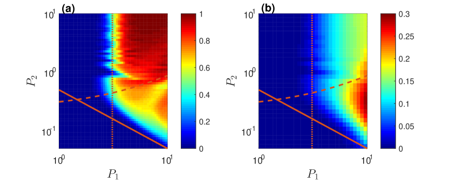
Figure 3: Color coded excitation efficiency from simulations in $P_{1,2}$ parameter space. The left panel represents simulations starting in the ground state without RWA, while the right panel shows the results for a thermal initial condition with $l_{c}=11.5$ and using the RWA. The final chirp time is $\tau_{f}=99P_{2}$ , which corresponds to $l_{f}=50$. The different lines show the quantum-classical boundary (dashed line), efficient LC threshold (dotted line) and AR boundary (solid line).

Here we discuss the efficiency of rotational excitation in the OC under two distinct initial conditions as illustrated in Figures 1 and 2, i.e. starting either in the ground state ($l_{c}=0$) or a ”hot” thermal ensemble ($l_{c}=11.5$), respectively. The latter value of $l_{c}$ is characteristic of existing experiments, such as in $N_{2}$ or $O_{2}$ at room temperature Milner1 . We define the excitation efficiency as the fraction of rotationally excited molecules within $20\%$ from the final target state $l_{f}=\frac{1}{2}+\frac{\tau_{f}}{2P_{2}}$, $\tau_{f}$ being the final driving time. Figures 3a and 3b show numerically found excitation efficiency for the ground-state initial condition and for the thermal initial ensemble, respectively (note that the color scales in the two figures are different). The final driving time in these examples is $\tau_{f}=99P_{2}$ corresponding to the resonant transition $l=48\rightarrow l=50$ ($l_{f}=50)$, so we used the fraction of the molecules excited beyond $\widehat{l}=0.8l_{f}=40$ in defining the excitation efficiency $f$. We show the quantum/classical separation boundary (7) (dashed line), as well as the autoresonance boundary line (10) (solid line) in both figures bounding the domains of different resonant excitation mechanisms. The value of $P_{1}\approx 3.1$ for which $f=0.5$ according to Eq. (9) can serve as the threshold for high excitation efficiency in the LC regime. We show this value of $P_{1}$ in Fig. 3 by the vertical dotted lines.

We discuss the ground state initial condition (Fig. 3a) first. Note that in the quantum region in this case (above the quantum/classical separation line), the resonant excitation efficiency increases with $P_{1}$, is almost independent of $P_{2}$, and can reach nearly $100\%$. This can be explained via the LC arguments. Indeed, for calculating the efficiency $f$ in this case one uses Eq. (9) with $C=0$. Figure 4 compares the prediction of Eq. (9) with simulations for $P_{2}=10$ (quantum regime) and three values of the final driving time defined by the target states $l_{f}=20$ (blue diamonds, dashed line), $50$ (orange circles, solid line), and $100$ (red squares, dotted line). All cases show good agreement between theory and simulations, demonstrating the validity of the RWA, and the possibility of very high (nearly $100\%$) excitation efficiencies for sufficiently large $P_{1}$. Nonetheless, for a given $P_{1}$, increasing the target state $l_{f}$ reduces the excitation efficiency because more population is left behind as the number of the successive LZ steps grows. This situation differs significantly from the classical AR, where molecules trapped in the rotational resonance are not lost and, in principle, can increase their rotational energy indefinitely as the laser pulse chirp continues, until other effects become important. If one starts from the ground state in the classical domain of parameters $P_{1,2\text{ }}$in 3a, the RWA is not valid, and nonresonant transitions, which break the conservation of $C=l-m$ play a key role in the removal of population from the resonant pathway. Nevertheless, the autoresonant boundary line serves as a threshold for efficient rotational excitation even for this initial condition despite its initial quantum nature. This case is illustrated in a video (See Supplemental Material Movies ) showing the evolution of rotational population in the $l,m$ space, for parameters identical to those of Fig. 1c.

.

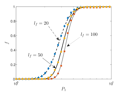
Figure 4: The OC excitation efficiency from numerical simulations for the ground-state initial condition (markers) and the theoretical prediction, Eq. (9) (lines). The parameter $P_{2}=10$ is kept constant, while the final $l_{f}$=$20$ (blue diamonds, dashed line), $50$ (orange circles, solid line), and $100$ (red squares, dotted line).

In the case of a thermal initial state, the classical region of the parameter space exhibits the highest resonant excitation efficiency. The latter is described by the classical theory of Ref. OurPaper (see Eq. (28) in that paper). This theory uses an additional weak drive assumption, which in terms of the parameters of the present work can be written as $\sqrt{\frac{2}{l_{c}\left(l_{c}+1\right)}\frac{P_{1}}{P_{2}}}\ll 1$ (note that $\hbar$ cancels out in this expression). Figure 5 compares the OC excitation efficiency in simulations using quantum mechanical formalism with (blue diamonds) and without (red pentagrams) RWA with the predictions of the classical theory (lines) and Monte Carlo simulations (orange squares). We used $l_{c}=11.5$, and $P_{2}=0.23$ (filled markers, solid line) and $0.1$ (empty markers, dashed line) in these calculations. The agreement with the classical theory of OurPaper is quite good for $P_{2}=0.23$, but not as good for $P_{2}=0.1$, because of the breaking of the weak drive assumption. Nevertheless, the classical Monte-Carlo simulations (orange squares) show good agreement with the quantum simulations even for $P_{2}=0.23$, which is close to the quantum/classical separation line. As expected, when the value of $P_{2}$ is decreased, the agreement between the simulations gets better. Note that while the RWA is not strictly valid in the region of the parameter space in these simulations, the results with and without RWA show good agreement due to the considerations described at the end of subsection III.1. Consequently, we have used the RWA in simulations in Fig. 3b, allowing a significant reduction of numerical complexity of quantum simulations (see appendix B). To the best of our knowledge, there is no analytic theory for calculating the excitation efficiency in the quantum region for initially thermal ensembles. Nevertheless, the evolution in this regime has the characteristics of LC, as exemplified in Fig. 2b and in a movie (See Supplemental Material Movies ) showing the evolution for the same parameters in the $l,m$ space. The successive LC transitions still take place, but now there exists a width in $C=l-m$. Note that the width in $l$ as seen in the simulations of the moving resonant bunch, is actually two different resonant pathways experiencing LC, each representing the conserved parity of $l$.

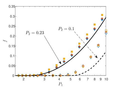
Figure 5: The excitation efficiency for a thermal ensemble from numerical simulations with all parameters identical to those in in Fig. 3, but $P_{2}=0.23$ (filled markers) and $0.1$ (empty markers). The markers show three different simulations: with RWA (blue diamonds), without RWA (red pentagram), and the classical Monte-Carlo simulation (orange squares), while the lines are theoretical predictions from OurPaper .

III.3 Relevance to existing experiments

Lastly, it is important to discuss our analysis in the context of existing experimental setups. Characteristic value of the chirp rate $\beta$ in these setups is $1ps^{-2}$ (see, for example, beta1 ; beta2 ). With this value of $\beta$, and the molecules already in use in OC experiments Corkum2 ; ExpRes ; beta2 , parameter $P_{2}$ (see Eq. 2) varies from $11.2$ (for $Cl_{2}$) through $0.73$ ($N_{2}$) to $0.09$ ($D_{2}$). These three values are represented by horizontal lines in Fig 6 in the $P_{1,2}$ parameter space. In the same figure, we also show the AR and LC domains (shaded blue areas) as discussed above. Clearly, these different resonant regimes are accessible in experiments. One can also see that in the $D_{2}$ and $N_{2}$ cases, one can exploit both the  AR and LC by a proper choice of $P_{1}$, while $Cl_{2}$ can not exhibit quantum LC dynamics.

To further exploit our analysis, we address the experimental results of Ref. ExpRes . The experiment involved $N_{2}$ molecules ($P_{2}=0.73$) and the OC laser pulse had a varying amplitude of a Gaussian form, $P_{1}=P_{10}\exp(-\tau^{2}/2\sigma^{2})$, $\sigma=52$ with $\tau$ starting from zero Valery . The lower panel in Fig. 10.8 of ExpRes shows two results with very different $l-$width of the excited bunch of molecules, with the narrow bunch corresponding to the laser pulse truncated at $\tau\approx 97$. Our analysis suggests the following interpretation of these results. If initially the system evolves in the efficient LC regime, the excited bunch is narrow (2-3 excited $l$ states). As parameter $P_{1}$ decreases, one crosses the efficient LC excitation threshold (vertical dotted line in Fig. 6) at some time and, as a result, more and more population leaves the resonant bunch and stays behind, until the bunch vanishes completely. This leads to a broad (non resonant) excited population. However, if one truncates the laser pulse at earlier time, the population freezes and the bunch remains narrow. To check this hypothesis, we have used our simulations and present the results in Fig. 7. The upper and the lower panels in the figure show the distribution $P\left(l\right)$ with and without the truncation, respectively. In this simulation $P_{10}=6$ and the system evolves in the $P_{1,2}$ parameter space along the thick part of the $N_{2}$ line in Fig. 6. One can observe formation of either narrow or wide excited bunches similar to the experimental results ExpRes .

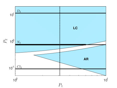
Figure 6: The $P_{1,2}$ parameter space with shaded areas dividing it into AR and LC regimes. The value of $P_{2}$ for $\beta=1ps^{-2}$ and $D_{2}$, $N_{2}$ and $Cl_{2}$ molecules is represented by the horizontal solid lines. The dotted line shows the efficient LC threshold, while the thick part of the $N_{2}$ line represents the trajectory of the simulationss in Fig. 7.

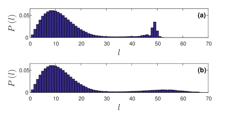
Figure 7: The distributions $P\left(l\right)$ in simulations with truncation of the laser pulse (panel a), and without the truncation (panel b).

IV SUMMARY

In conclusion, we have studied the problem of resonant rotational excitation in the optical centrifuge for a wide range of parameters starting from either the ground-state or a ”hot” thermal ensemble. Based on three characteristic time scales in the problem, we introduced two dimensionless parameters $P_{1,2}$, and studied the resonant nature of the problem in the parameters space by using the rotating wave approximation. We have shown how two distinct resonant regimes can appear in this problem, i.e the quantum mechanical ladder-climbing and the classical autoresonance and discussed a separation criterion between the two regimes in the $P_{1,2}$ parameter space.

We have also derived criteria for efficient rotational excitation in the OC for the two resonant mechanisms and have shown that both are present with the aforementioned initial conditions, but their manifestation is different. Indeed, the maximal resonant excitation efficiency is significantly higher with the ground-state initial condition. Furthermore, the most efficient excitation mechanism is the ladder climbing in the case of the ground-state initial condition, while it’s the classical autoresonance when starting with the thermal ensemble. When possible, the excitation efficiency in simulations was compared to theoretical predictions. Our current theoretical understanding allows calculation of the excitation efficiency in the most efficient regime for each of the above initial conditions. The validity of the rotating wave approximation and quantum/classical correspondence was also studied analytically and numerically.

The results of this work combine the classical OurPaper and the quantum formalisms, broadening the previous analysis of the OC problem, which did not address the full complexity of the quantum case, especially dealing with thermal initial conditions OCtheory3 . These results address main issues associated with the efficiency and the spectral width of the excited resonant bunch of molecules in the OC, which is important in planning future experiments. We have also shown that existing experimental setups can access different resonant regimes of operation studied in this work by using light and heavy molecules, varying gas temperature, and laser intensity. While the analysis presented here assumes rigid rotor molecules, some effects of nonrigidity could be studied similarly in the future. For example, the limitation on parity of $l,m$ due to spin-statistics in some molecules does not change the analysis. On the other hand, the centrifugal radial expansion adds a third parameter to the problem, representing the $\propto l^{2}\left(l+1\right)^{2}$ addition to the energy. Since this effect continuously increases the time between the resonant transitions, it may allow a forced dynamical transition from classical autoresonance to quantum ladder-climbing in the process of the same continuing rotational excitation.

Appendix A Quantum mechanical coupling

Using the parameterization of Sec. II, the dimensionless evolution equation for the coefficients $a_{l,m}$ is:

$$i\frac{da_{l,m}}{d\tau}=E_{l}a_{l,m}+\left\langle l,m\right|\hat{U}\sum_{k,s}a_{k,s}\left|k,s\right\rangle.$$ (11)

Here we expand the dimensionless interaction energy $U$ in spherical harmonics $Y_{l}^{m}\left(\theta,\phi\right)$:

$$U=-P_{1}\left[\sqrt{\frac{2\pi}{15}}\left(Y_{2}^{2}e^{-2i\phi_{d}}+Y_{2}^{-2}e^{2i\phi_{d}}\right)-\sqrt{\frac{4\pi}{45}}Y_{2}^{0}+\frac{1}{3}\right].$$ (12)

Then, the inner product in Eq. (11) can be expressed as the integral of three spherical harmonics, and represented via the Wigner 3-j symbol. The selection rules for the quantum mechanical transitions occur naturally from the selection rules of the 3-j symbol, while the coupling coefficients $c_{l,m}^{\Delta l,\Delta m}$ can be calculated directly. We summarize these coefficients (up to the phase term which was included explicitly in Eq. (3)) in table 1.

Table 1: Coupling coefficient for the transition $\left|l,m\right>\rightarrow\left|l+\Delta l,m+\Delta m\right>$

$\Delta l$	$\Delta m$	$c^{\Delta l,\Delta m}_{l,m}$
$0$	$0$	$-\frac{1}{3}\left[1-\frac{l^{2}+l-3m^{2}}{\left(2l-1\right)\left(2l+3\right)}\right]$
$2$	$0$	$\frac{1}{2}\sqrt{\frac{\left(l-m+1\right)\left(l-m+2\right)\left(l+m+1\right)\left(l+m+2\right)}{\left(2l+1\right)\left(2l+3\right)^{2}\left(2l+5\right)}}$
$-2$	$0$	$\frac{1}{2}\sqrt{\frac{\left(l-m-1\right)\left(l-m\right)\left(l+m-1\right)\left(l+m\right)}{\left(2l+1\right)\left(2l-1\right)^{2}\left(2l-3\right)}}$
$0$	$2$	$\frac{1}{2}\frac{\sqrt{\left(l+m+1\right)\left(l+m+2\right)\left(l-m-1\right)\left(l-m\right)}}{\left(2l-1\right)\left(2l+3\right)}$
$0$	$-2$	$\frac{1}{2}\frac{\sqrt{\left(l-m+1\right)\left(l-m+2\right)\left(l+m-1\right)\left(l+m\right)}}{\left(2l-1\right)\left(2l+3\right)}$
$2$	$2$	$-\frac{1}{4}\sqrt{\frac{\left(l+m+1\right)\left(l+m+2\right)\left(l+m+3\right)\left(l+m+4\right)}{\left(2l+1\right)\left(2l+3\right)^{2}\left(2l+5\right)}}$
$2$	$-2$	$-\frac{1}{4}\sqrt{\frac{\left(l-m+1\right)\left(l-m+2\right)\left(l-m+3\right)\left(l-m+4\right)}{\left(2l+1\right)\left(2l+3\right)^{2}\left(2l+5\right)}}$
$-2$	$2$	$-\frac{1}{4}\sqrt{\frac{\left(l-m\right)\left(l-m-1\right)\left(l-m-2\right)\left(l-m-3\right)}{\left(2l+1\right)\left(2l-1\right)^{2}\left(2l-3\right)}}$
$-2$	$-2$	$-\frac{1}{4}\sqrt{\frac{\left(l+m\right)\left(l+m-1\right)\left(l+m-2\right)\left(l+m-3\right)}{\left(2l+1\right)\left(2l-1\right)^{2}\left(2l-3\right)}}$

Appendix B Numerical simulations

Our numerical simulations when starting in the ground state used Eq. (3). Because of the preferred resonant transition $\left|l,m\right\rangle\rightarrow\left|l+2,m+2\right\rangle$, even for large time intervals, the value of $C=l-m$ remained bounded throughout the evolution (even when the RWA fails initially). Therefore, for faster simulations, a maximum value $C_{max}$ was chosen and only states with $C\leq C_{max}$ were taken into account. Furthermore, due to the parity conservation of $l,m$, only states with even $l,m$ were considered.

For the thermal state initial condition, the von Neumann equation was solved

$$i\frac{d\rho}{d\tau}=[H,\rho],$$ (13)

where $\rho$ is the density matrix, $H$ the dimensionless Hamiltonian and the brackets denote the commutator. In the basis of the eigenstates $\left|l,m\right\rangle$ the coupling matrix is identical to that derived for Eq. (3). Again, a maximum value $C_{max}$ was used, and the computation was carried out independently for each of the four conserved parity combinations of $l,m$. Due to the increased order of the ODE, in several cases the simulations used the RWA coupling instead. In this case and due to the conservation of $C=l-m$, the calculation was done using independent ”chains” of equal $C$ values, up to $C_{max}$ and according to the different parity choices for $l,m$. In all simulations the final time of the simulation was taken to be large enough, so that a clear separation was achieved between the population around the target state and that left in the lower $l$ states. This is especially important for values of $P_{1}P_{2}$ near the threshold $1/2$, where such separation is hard to achieve. The numerical uncertainty in Figs. 4,5 is smaller than the marker sizes.

References

- (1) B.V. Chirikov, Phys. Rep. 52, 263 (1978).
- (2) A. J. Lichtenberg and M. A. Lieberman, Regular and Stochastic Motion (Springer-Verlag, New York, 1983).
- (3) R. Z. Sagdeev, D. A. Uzikov, and Cr. M. Zaslavsky, Non linear Physics. From the Pendulum to Turbulence and Chaos (Harwood Academic, Chur, 1988).
- (4) R. Bluemel, S. Fishman, and U. Smilansky, J. Chem. Phys. 84, 2604 (1986).
- (5) J. Floß, S. Fishman, and I. Sh. Averbukh, Phys. Rev. A 88, 023426 (2013).
- (6) M. Bitter and V. Milner, Phys. Rev. Lett. 117, 144104 (2016).
- (7) J. Karczmarek, J. Wright, P. Corkum, and M. Ivanov, Phys. Rev. Lett. 82, 3420 (1999).
- (8) D. M. Villeneuve, S. A. Aseyev, P. Dietrich, M. Spanner, M. Yu. Ivanov, and P. B. Corkum, Phys. Rev. Lett. 85, 542 (2000).
- (9) L. Yuan, S. W. Teitelbaum, A. Robinson, and A. S. Mullin, Proc. Natl. Acad. Sci. USA 108, E17 (2011).
- (10) A. Korobenko, A. A. Milner, and V. Milner, Phys. Rev. Lett. 112, 113004 (2014).
- (11) A. A. Milner, A. Korobenko, J. W. Hepburn, and V. Milner, Phys. Rev. Lett. 113, 043005 (2014).
- (12) A. A. Milner, A. Korobenko, K. Rezaiezadeh, and V. Milner, Phys. Rev. X 5, 031041 (2015).
- (13) A. A. Milner, A. Korobenko, and V. Milner, Phys. Rev. Lett. 118, 243201 (2017).
- (14) J. Fajans and L. Friedland, Am. J. Phys. 69, 1096-1102 (2001).
- (15) L. D. Landau, Phys. Z. Sowjetunion 2, 46 (1932).
- (16) C. Zener, Proc. R. Soc. London A 137, 696 (1932).
- (17) S. Chelkowski and G. N. Gibson, Phys. Rev. A 52, R3417 (1995).
- (18) D. Maas, D. Duncan, R. Vrijen, W. Van Der Zande, and L. Noordam, Chem. Phys. Lett. 290, 75 (1998).
- (19) G. Marcus, A. Zigler, and L. Friedland, Europhys. Lett. 74, 43 (2006).
- (20) G. Marcus, L. Friedland, and A. Zigler, Phys. Rev. A 69, 013407 (2004).
- (21) E. Grosfeld and L. Friedland, Phys. Rev. E 65, 046230 (2002).
- (22) Y. Shalibo, Y. Rofe, I. Barth, L. Friedland, R. Bialczack, J.M. Martinis, and N. Katz, Phys. Rev. Lett. 108, 037701 (2012).
- (23) I. Barth, I. Y. Dodin, and N. J. Fisch, Phys. Rev. Lett. 115, 075001 (2015).
- (24) K. Hara, I. Barth, E. Kaminski, I. Y. Dodin, and N. J. Fisch, Phys. Rev. E 95, 053212 (2017).
- (25) G. Manfredi, O. Morandi, L. Friedland, T. Jenke, and H. Abele, Phys. Rev. D 95 025016 (2017).
- (26) I. Barth, L. Friedland, O. Gat, and A.G. Shagalov, Phys. Rev. A 84, 013837 (2011).
- (27) T. Armon and L. Friedland, Phys. Rev. A 93, 043406 (2016).
- (28) M. Spanner and M. Y. Ivanov, J. Chem. Phys. 114, 3456 (2001).
- (29) M. Spanner, K. M. Davitt, and M. Y. Ivanov, J. Chem. Phys. 115, 8403 (2001).
- (30) N. V. Vitanov and B. Girard, Phys. Rev. A 69, 033409 (2004).
- (31) J. J. Sakurai and S. F. Tuan, Modern quantum mechanics (Addison-Wesley, Reading, MA 1994), pp. 195-203.
- (32) Note, that a term of was omitted from the function in Eq. (7) of OurPaper as it carried no classical meaning.
- (33) See Supplemental Material at http://link.aps.org/supplemental/10.1103/PhysRevA.96.033411 for “Movie1” and “Movie2” for the evolution of the population in the l,m space, for parameters identical to those of Fig. 1(c) and Fig. 2(b).
- (34) A. Korobenko, A. A. Milner, J. W. Hepburn and V. Milner, Phys. Chem. Chem. Phys. 16, 4071 (2014).
- (35) A. Korobenko, J. W. Hepburn and V. Milner, Phys. Chem. Chem. Phys. 17, 951 (2015).
- (36) V. Milner, and J. W. Hepburn, Laser Control of Ultrafast Molecular Rotation, in Advances in Chemical Physics Vol. 159 (eds P. Brumer, S. A. Rice and A. R. Dinner), (John Wiley & Sons, Inc, Hoboken, NJ 2016) .
- (37) V. Milner, University of British Columbia, Vancouver, Canada (Private communication).