Tachyon Logamediate inflation on the brane

Abstract

According to a Barrow’s solution for the scale factor of the universe, the main properties of the tachyon inflation model in the framework of RSII braneworld are studied. Within this framework the basic slow-roll parameters are calculated analytically. We compare this inflationary scenario against the latest observational data. The predicted spectral index and the tensor-to-scalar fluctuation ratio are in excellent agreement with those of Planck 2015. The current predictions are consistent with those of viable inflationary models.

1 The set up and motivation:

Standard model of inflation is driven by an scalar inflaton (quanta of the inflationary field) fields follow back to early efforts to solve the basic problems of the Big-Bang cosmology, namely horizon, flatness and monopoles Guth (1981); Albrecht and Steinhardt (1982). The nominal inflationary paradigm contains two mainly different segments: the slow-roll and the (P)reheating regimes. In the slow-roll phase the kinetic part of energy (which has the canonical form here) of the scalar field is negligible with respect to the potential part of energy $V(\phi)$ which implies a nearly deSitter expansion of the Universe. However, after the slow-roll epoch the kinetic energy becomes comparable to the potential energy and thus the inflaton field oscillates around the minimum at the (P)reheating phase and progressively the universe is filled by radiation Shtanov et al. (1995); Kofman et al. (1997). In order to achieve inflation one can use tachyon scalar fields for which the kinetic term does not follow the canonical form (k-inflation Armendariz-Picon et al. (1999)). It has been found that tachyon fields which are associated with unstable D-branes Sen (2002a) may be responsible for the cosmic acceleration phase in early times Sen (2002b); Sami et al. (2002); Armendariz-Picon et al. (1999). Notice, that tachyon potential has the following two properties: the maximum of the potential occurs when $\phi\rightarrow 0$ while the corresponding minimum takes place when $\phi\rightarrow\infty$. For tachyonic models of inflation with ground state at $\phi\rightarrow\infty$, inflaton rolls toward its ground state without oscillating about it and the reheating mechanism does not work Kofman and Linde (2002). For quasi power-low time dependence, which will be considered in the present work, there is a weak scale factor dependence of the tachyon energy density. Therefore in the post-inflation era the tachyon density would always dominate radiation unless there is a mechanism by which tachyon decay into radiation. Our tachyon model in the present work is an unphysical toy model but there is a solution for reheating problem in the context of warm inflationSetare and Kamali (2012, 2013a, 2014a, 2014b, 2013b); Kamali et al. (2016, 2017); Basilakos et al. (2017), which however is beyond the scope of the present work. From the dynamical viewpoint one may present the equation of motion of tachyon field using a special Lagrangian Gibbons (2002) which is non-minimally coupled to gravity:

$$L=\sqrt{-g}\left[\frac{R}{16\pi G}-V(\phi)\sqrt{1-g^{\mu\nu}\partial_{\mu}\phi\partial_{\nu}\phi}\right]\;.$$ (1)

Considering a spatially flat $Friedmann-Lemaitre-Robertson-Walker$ (FLRW) (hereafter FLRW) universe the stress-energy tensor components are presented by

$$T^{\mu}_{\nu}=\frac{\partial L}{\partial(\partial_{\mu}\phi)}\partial_{\nu}\phi-g^{\mu}_{\nu}L={\rm diag}(-\rho_{\phi},p_{\phi},p_{\phi},p_{\phi})$$ (2)

equation where $\rho_{\phi}$ and $p_{\phi}$ are the energy density and pressure of the tachyon field. Combining the above set of equations one can find

$$\rho_{\phi}=\frac{V(\phi)}{\sqrt{1-\dot{\phi}^{2}}}$$ (3)

and

$$P_{\phi}=-V(\phi)\sqrt{1-\dot{\phi}^{2}}$$ (4)

Where $\phi$ is tachyon scalar field in unite of inverse Planck mass $M_{pl}^{-1}$, and $V(\phi)$ is potential associated with the tachyon scalar field. In the past few years, there was a debate among particle physicists and cosmologists regarding those phenomenological models which can be produced in extra dimensions. For example, the reduction of higher-dimensional gravitational scale, down to TeV-scale, could be presented by an extra dimensional scenario Arkani-Hamed et al. (1998, 1999); Antoniadis et al. (1998). In these scenarios, gravity field propagates in the bulk while standard models of particles are confined to the lower-dimensional brane. In this framework, the extra dimension induces additional terms in the first Friedmann equation Binetruy et al. (2000a, b); Shiromizu et al. (2000). Especially, if we consider a quadratic term in the energy density then we can extract an accelerated expansion of the early universe Maartens et al. (2000); Cline et al. (1999); Csaki et al. (1999); Ida (2000); Mohapatra et al. (2000). We will study tachyon inflation model in the framework of Randall-Sundrum II braneworld Randall and Sundrum (1999) which contains a single, positive tension brane and a non-compact extra dimension. We note that this is not the only scenario in where these characteristics are presented. For example DBI Galileon inflation Silverstein and Tong (2004); Alishahiha et al. (2004); Martin and Yamaguchi (2008); Guo and Ohta (2008) has these properties in its $T_{3}$ brane and cosmological inflation analysis of this model agrees with $1\sigma$ confidence level of Planck data Kumar et al. (2016). Following the lines of Ref.Ravanpak and Salmeh (2014), we attempt to study the main properties of the tachyon inflation in which the scale factor evolves as $a(t)\propto\exp(A[\ln t]^{\lambda})$, where $\lambda>1$ and $A>0$ ("Logamediate inflation"). For $\lambda=1$ case cosmic expansion evolves as ordinary power-law inflation $a\propto t^{p}$ where $p=A$ Barrow (1996); Barrow and Nunes (2007). More details regarding the cosmic expansion in various inflationary solutions can be found in the papers by Barrow Barrow (1996); Barrow and Nunes (2007). In these papers there is no comment about the behaviour around $\lambda=0$ case of logamediate solution. In the current work, we investigate the possibility of using the logamediate solution in the case of tachyon inflation on the brane. Specifically, the structure of the article is as follows: In section II we briefly discuss the main properties of the tachyon inflation, while in section III we provide the perturbation parameters. In section IV we study the performance of our predictions against the Planck 2015 data. Finally, the main conclusions are presented in section VI.

2 Tachyon inflation

In this part we consider a FLRW universe with tachyon component in inflation era, the basic cosmological equations in the context of the Randall-Sundrum II (RSII) brane Randall and Sundrum (1999) are presented as:

$$H^{2}=\frac{1}{3}\rho_{\phi}(1+\frac{\rho_{\phi}}{2\tau}),$$ (5)

$${\dot{\rho}}_{\phi}+3H(\rho_{\phi}+p_{\phi})=0$$ (6)

and

$$\dot{H}=-\frac{1}{2M_{p}^{2}}(\rho_{\phi}+P_{\phi})(1+\frac{\rho_{\phi}}{\tau})$$ (7)

where $H=\frac{\dot{a}}{a}$ and $a$ are Hubble parameter and scale factor respectively, dot means derivative with respect to the cosmic time. Parameter $\tau$ in Eq.(5) represents the brane tension Shiromizu et al. (2000); Binetruy et al. (2000a, b). The value of this term is constrained, to be $\tau>(1MeV)^{4}$ by considering nucleosynthesis epoch Cline et al. (1999). Another stronger limitation for the value of $\tau$ is presented by usual tests for deviation from Newton’s law $\tau\geq(10Tev)^{4}$ Brax and van de Bruck (2003). The model is considered in natural unit $8\pi G=\frac{h}{2\pi}=c=1$. Using Eqs.(3,4,5,6,7), we can derive background evolution motions of tachyon scalar field coupled by scale factor in high energy limit $\rho_{\phi}\gg\tau$.

$$3H^{2}=\frac{V^{2}(\phi)}{2\tau\sqrt{1-\dot{\phi}^{2}}}~{}~{}~{}~{}~{}~{}~{}~{}~{}$$ (8)

$$\frac{\ddot{\phi}}{1-\dot{\phi}^{2}}+3H\dot{\phi}+\frac{1}{V}\frac{dV}{d\phi}=0\;,$$

$$\dot{H}=-\frac{\rho^{2}\dot{\phi}^{2}}{2M_{p}^{2}\tau}~{}~{}~{}~{}~{}~{}~{}~{}~{}~{}~{}~{}~{}~{}~{}$$

In Ref.Barrow and Nunes (2007), a complete analysis around the slow-roll parameters was made for canonical scalar fields which leads to slow-roll condition $3H\dot{\phi}\simeq-\frac{dV(\phi)}{d\phi}$. We will consider our model in slow-roll limit of tachyonic scalar fields ,$\dot{\phi}\ll 1$   $\ddot{\phi}\ll 3H\dot{\phi}$ which leads to $3HV\dot{\phi}\simeq-\frac{dV(\phi)}{d\phi}$ Fairbairn and Tytgat (2002). In the slow-roll regime of tachyon fields, from relations (8) $\dot{\phi}$ can be presented in term of Hubble parameter and its derivative:

$$\dot{\phi}=\sqrt{-\frac{\dot{H}}{3H^{2}}}$$ (9)

which will be used in our future purposes. Using Eqs.(7) and (8) we can find a real velocity field $\dot{\phi}$ in Eq.(9). Now we consider logamediate inflation model in which its scale factor behaves as Barrow (1996); Barrow and Nunes (2007):

$$a(t)=a_{0}\exp(A[\ln t]^{\lambda})\;,$$ (10)

one can present the compact solution of Eq.(9).

$$\frac{d\phi}{dt}\simeq\sqrt{\frac{1}{A\lambda(\ln t)^{\lambda-1}}},\Rightarrow\phi-\phi_{0}=\frac{1}{\sqrt{A\lambda}}\int(\ln t)^{\frac{1-\lambda}{2}}dt$$ (11)

which leads to

$$\phi=\phi_{0}+\frac{g(t)}{K}~{}~{}~{}~{}~{}~{}~{}~{}~{}~{}~{}$$ (12)

$$g(t)=\gamma(\frac{3-\lambda}{2},-\ln t)$$

where $K=\sqrt{3\lambda A}$ and $\gamma(a,x)$ is incomplete gamma function Arfken (1985); M. Abramowitz (1972), where $a$ is an integer constant and $x$ is a variable, for example in our case $(a,x)=(\frac{3-\lambda}{2},-\ln t)$ . Dimensionless slow-roll parameters of the model can be introduced by standard definition in term of scalar field

$$\epsilon=-\frac{\dot{H}}{H^{2}}=\frac{[\ln(g^{-1}[K(\phi-\phi_{0})])]^{1-\lambda}}{\lambda A}~{}~{}~{}~{}~{}~{}~{}~{}~{}~{}~{}~{}~{}~{}~{}~{}~{}~{}$$ (13)

$$\eta=\frac{1}{2H}[-\frac{\ddot{V}}{\dot{V}}+\frac{\dot{H}}{H}+\frac{\dot{V}}{V}]=\epsilon[-1+\frac{1}{g^{-1}[K(\phi-\phi_{0})]}]$$

where $g^{-1}(t)$ is inverse function of $g(t)$. In the above relations we have used the approximation, $\ln t\gg\lambda-1$ which may be used at the early time. Number of e-folding can be presented for the model

$$N=\int_{t_{1}}^{t}Hdt^{\prime}=\int_{\phi_{1}}^{\phi}\frac{H}{\dot{\phi^{\prime}}}d\phi^{\prime}~{}~{}~{}~{}~{}~{}~{}~{}~{}~{}~{}~{}~{}~{}~{}~{}$$ (14)

$$N=(\ln[g^{-1}(K[\phi-\phi_{0}])])^{\lambda}-(\lambda A)^{\frac{\lambda}{1-\lambda}}$$

where $\phi_{1}$ is introduced at the beginning of the inflation when the $\epsilon=1$. Using Eq.(14) we can find tachyon scalar field in term of variable number of e-fold $N$

$$\phi=\phi_{0}+g[\exp([N+(\lambda A)^{\frac{\lambda}{1-\lambda}}]^{\frac{1}{\lambda}})]$$ (15)

which will be used for the future goals. Potential of tachyon filed may be presented by using Eq.(8)

$$V(\phi)=6\tau(\lambda A)^{2}\frac{(\ln g^{-1}[K(\phi-\phi_{0})])^{2(\lambda-1)}}{(g^{-1}[K(\phi-\phi_{0})])^{2}}$$ (16)

3 Perturbation

Although assuming a spatially-flat, isotropic and homogeneous FRW universe may be useful and reasonable, but there are observed deviations from isotropic and homogeneity in our universe. These deviations motivate us to use perturbation theory in cosmology. In the context of general relativity and gravitation, inhomogeneity grows with time, so it was very small in the past time. Therefore first order or linear perturbation theory can be used for scalar field models at the inflation epoch. Considering Einstein’s equation, inflaton field in the FRW universe connects to the metric components of this universe, so Perturbed inflaton field must be studied in the perturbed FRW geometry. Most general linear perturbation of spatially-flat FRW metric is presented by:

$$ds^{2}=-(1+2C)dt^{2}+2a(t)D_{,i}dx^{i}dt~{}~{}~{}~{}~{}~{}~{}~{}~{}~{}~{}~{}~{}$$ (17)

$$+a^{2}(t)[(1-2\psi)\delta_{ij}+2E_{,ij}+2h_{ij}]dx^{i}dx^{j}$$

which includes scalar perturbations $C,D,\psi,E$ and traceless-transverse tensor perturbations $h_{ij}$. Power-spectrum of the curvature perturbation $P_{R}$, that is derived from correlation of first order scalar field perturbation in vacuum state can be constrained by observational data. For tachyon fields, this parameter at the first level is presented by Hwang and Noh (2002); Ravanpak and Salmeh (2014)

$$\mathcal{P}_{R}=(\frac{H^{2}}{2\pi\dot{\phi}})^{2}\frac{1}{V(1-\dot{\phi}^{2})^{\frac{3}{2}}}$$ (18)

This parameter is essential for our perturbed analysis which is presented in Ref.Hwang and Noh (2002). In slow-roll and high energy limit, using Eq.(8), we may simplify the above relation as:

$$\mathcal{P}_{R}=\frac{1}{4\pi^{2}V}(\frac{V^{2}}{2\tau V^{\prime}})^{2}~{}~{}~{}~{}~{}~{}~{}~{}~{}~{}~{}~{}~{}~{}~{}~{}~{}~{}~{}~{}~{}~{}$$ (19)

$$\simeq\frac{3(A\lambda)^{6}}{4\pi^{2}\sqrt{6\tau}}\exp(-(\frac{N}{A})^{\frac{1}{\lambda}})(\frac{N}{A})^{\frac{4(\lambda-1)}{\lambda}}$$

where $V^{\prime}=\frac{dV}{d\phi}$. Another two important perturbation parameters are spectral index $n_{s}=1+\frac{d\ln P_{R}}{d\ln k}$ and its running $n_{run}=\frac{dn_{s}}{d\ln k}$. From Eq.(18) in the slow-roll limit, these parameters are presented by

$$n_{s}=1+2\epsilon[-2+\frac{1}{g^{-1}(K[\phi-\phi_{0}])}]\simeq 1+\frac{4(1-\lambda)}{\lambda}\frac{1}{N}$$ (20)

$$n_{run}=\frac{4(\lambda-1)}{(\lambda A)^{2}}(\ln g^{-1}[K(\phi-\phi_{0})])^{1-2\lambda}~{}~{}~{}~{}~{}~{}~{}~{}~{}~{}~{}~{}~{}~{}~{}~{}~{}~{}$$

These parameters also may be constrained by observational data. Up to now, we consider scalar perturbation parameters. During inflation era, there are two independent components of gravitational waves $h_{+},h_{\times}$ or tensor perturbation of the metric with the same equation of motion. Amplitude of the tensor perturbation is given by

$$\mathcal{P}_{g}=8(\frac{H}{2\pi})^{2}(\frac{3}{\tau^{2}})^{\frac{1}{4}}H^{\frac{1}{2}}=\frac{2}{\pi^{2}}(\frac{3}{6^{5}\tau^{7}})^{\frac{1}{4}}V^{\frac{5}{2}}$$ (21)

which have been presented in Ref.Langlois et al. (2000). Tensor-scalar ratio is another important parameter

$$r=\frac{\mathcal{P}_{g}}{\mathcal{P}_{R}}=(\frac{2\pi^{8}4^{3}}{3^{4}\tau^{7}})^{\frac{1}{4}}\frac{(2\tau V^{\prime})^{4}}{V^{\frac{9}{2}}}~{}~{}~{}~{}~{}~{}~{}~{}~{}~{}~{}~{}~{}~{}~{}~{}~{}~{}~{}~{}~{}~{}~{}~{}~{}~{}~{}~{}~{}$$ (22)

$$\simeq\frac{197}{K}(\frac{N}{A})^{\frac{\lambda-1}{2\lambda}}\exp(-\frac{3}{2}(\frac{N}{A})^{\frac{1}{\lambda}})~{}~{}~{}~{}~{}~{}~{}~{}~{}~{}~{}~{}~{}~{}~{}~{}~{}~{}~{}~{}~{}~{}~{}~{}~{}~{}~{}~{}~{}$$

$$=\frac{197}{K}(\frac{4(\lambda-1)}{a\lambda}\frac{1}{1-n_{s}})^{\frac{\lambda-1}{2\lambda}}\exp(-\frac{3}{2}(\frac{4(\lambda-1)}{A\lambda(1-n_{s})})^{\frac{1}{\lambda}})$$

$r-n_{s},$ trajectory for inflation models can be compared with Planck observational data.

4 Comparison with observation

The analysis of Planck data sets has been done in Ref.Ade et al. (2015a). The results of this analysis indicate the single scalar field models of inflation in slow-roll limit have limited spectral index, very low spectral running and tensor-scalar ratio.

$$n_{s}=0.968\pm 0.006~{}~{}~{}~{}~{}~{}~{}~{}~{}~{}~{}~{}~{}~{}~{}~{}~{}~{}$$ (23)

$$r=\frac{\mathcal{P}_{g}}{\mathcal{P}_{R}}<0.11,~{}~{}~{}~{}~{}~{}~{}~{}~{}~{}~{}~{}~{}~{}~{}~{}~{}~{}~{}~{}~{}~{}~{}$$

$$n_{run}=\frac{dn_{s}}{d\ln k}=-0.003\pm 0.007~{}~{}~{}~{}~{}$$

The upper bound set on tensor-scalar ratio function and running of the tensor-scalar ratio has been gained by using the results of Planck team and joint analysis of BICEP2/Keck Array/Planck Ade et al. (2015b). In the present section we will try to test the performance of tachyon inflation against the results of observation (23). In Fig.(1) we render the confidence contours in the $(n_{s},r)$ plane. The values of pair $(\lambda,A)$ are fixed for each trajectory. The curves are related to the pairs $(\lambda,A)$ as: $(29,4\times 10^{-12})$, $(39,10^{-15})$, $(19,3\times 10^{-6})$ and $(49,5\times 10^{-4})$ up to down. The main difference between our braneworld model and ordinary scalar field models Barrow (1996); Ravanpak and Salmeh (2014) is that there is no transition from $n_{s}<1$ to $n_{s}>1$ for all values of $\lambda$. For the big values of $\lambda$ with special combinations of $(\lambda,A)$ there are curves which behave as Harrison-zel’dovich spectrum i.e. $n_{s}=1$.

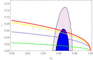
Figure 1: $1\sigma$ and $2\sigma$ confidence regions which borrowed from Planck Ade et al. (2014), $r-n_{s}$ trajectories of the present model. The solid red, dashed yellow, dotted blue and dot-ashed green lines correspond to combinations $(29,4\times 10^{-12})$, $(39,10^{-15})$, $(19,3\times 10^{-6})$ and $(49,5\times 10^{-4})$ of $(\lambda,A)$. There is no transition from $n_{s}<1$ to $n_{s}>1$.

In Fig.(2), the dot-dashed green line and dashed blue line are related to the pairs $(29,12\times 10^{-3}),(3,10^{-12})$ respectively. In this figure for the large value of $\lambda=69$ and small value of $A=10^{-50}$, the trajectory placed out of $95\%$ confidence which means large values of $\lambda$ are not compatible with Planck data.

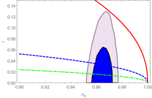
Figure 2: $1\sigma$ and $2\sigma$ confidence regions which borrowed from Planck Ade et al. (2014), $r-n_{s}$ trajectories of the present model. The dot-dashed green, dashed blue and solid red lines related to pairs $(29,12\times 10^{-3}),(3,10^{-12})$ and $(69,10^{-50})$. The trajectory placed out of $95\%$ confidence for the large value of $\lambda$.

In Figs.(1) and (2) the curves of our model compared with $68\%$ and $95\%$ confidence regions from Planck 2015 resultAde et al. (2015a) at $k_{*}=0.05Mpc^{-1}$.

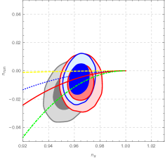
Figure 3: $n_{s}-n_{run}$ diagram. The area corresponds to Planck data and $n_{s}-n_{run}$ trajectories relate to our model. The dashed yellow, dotted blue, solid red, and dot-dashed green lines correspond to combinations: $(19,6\times 10^{-9})$, $(29,4\times 10^{-3})$, $(39,2\times 10^{-20})$, $(49,3\times 10^{-9})$

In Fig.(3), we plotted $n_{run}-n_{s}$ trajectories for some pairs $(\lambda,A)$ which have been used in previous figures. There is no running in the scalar spectral index for combination $(19,6\times 10^{-9})$.

5 Comparison with other models

Bellow we will compare the current predictions with those of viable literature potentials. This can help us to understand the variants of the tachyon-brane inflationary model from the observationally viable inflationary scenarios.

• The Starobinsky or $R^{2}$ inflation model Starobinsky (1980): In Starobinsky inflation model the asymptotic behavior of the effective potential is presented as $V(\phi)\propto[1-2\mathrm{e}^{-B\phi/M_{pl}}+\mathcal{O}(\mathrm{e}^{-2B\phi/M_{pl}})]$ which provides the following predictions in the slow-roll limitMukhanov and Chibisov (1981); Ellis et al. (2013): $r\approx 8/B^{2}N^{2}$ and ,$n_{s}\approx 1-2/N$ where $B^{2}=2/3$. Therefore, if we select $N=50$ then we obtain $(n_{s},r)\approx(0.96,0.0048)$. For $N=60$ we find $(n_{s},r)\approx(0.967,0.0033)$. It has been found that the Planck data Ade et al. (2015a) favors the Starobinsky inflation. Obviously, our results (see figures 1 and 2) are consistent with those of $R^{2}$ inflation.

• The chaotic model of inflation Linde (1983): In this inflationary model the potential is given by $V(\phi)\propto\phi^{k}$. The basic slow-roll parameters for this potential are presented as $\epsilon=k/4N$, $\eta=(k-1)/2N$ which leads to $n_{s}=1-(k+2)/2N$ and $r=4k/N$. It has been found that monomial potentials with $k\geq 2$ are not in agreement with the Planck data Ade et al. (2015a). Using $k=2$ and $N=50$ we present $n_{s}\simeq 0.96$ and $r\simeq 0.16$. For $N=60$ we find $n_{s}\simeq 0.967$ and $r\simeq 0.133$. It is interesting to note that this model also corresponds to the results of intermediate inflation Barrow (1990); Barrow and Liddle (1993); Barrow et al. (2006, 2014) with Hubble rate during inflation which is given by $H\propto t^{k/(4-k)}$ with $n_{s}=1-(k+2)r/8k$ and $k=-2$ case gives $n_{s}=1$ exactly to the first order.

• Hyperbolic model of inflation Basilakos and Barrow (2015): In hyperbolic inflation the potential is presented by $V(\phi)\propto\mathrm{sinh}^{b}(\phi/f_{1})$. Initially, this potential was proposed in the context of late time acceleration phase or dark energy Rubano and Barrow (2001). Recently, the properties of this scalar field potential have been investigated back in the inflationary epoch Basilakos and Barrow (2015) . The slow-roll parameters are written as

  $$\epsilon=\frac{b^{2}M_{pl}^{2}}{2f_{1}^{2}}\mathrm{coth}^{2}(\phi/f_{1}),$$

  $$\eta=\frac{bM_{pl}^{2}}{f_{1}^{2}}\left[(b-1)\mathrm{coth}^{2}(\phi/f_{1})+1\right]$$

  and

  $$\phi=f_{1}\;\mathrm{cosh}^{-1}\left[e^{NbM_{pl}^{2}/f^{2}}\mathrm{cosh}(\phi_{end}/f_{1})\right].$$

  where $\phi_{end}\simeq\frac{f}{2}\mathrm{ln}\left(\frac{\theta+1}{\theta-1}\right)$. Comparing this model with observational data, it has been found $n_{s}\simeq 0.968$, $r\simeq 0.075$, $1<b\leq 1.5$ and $f_{1}\geq 11.7M_{pl}$ Basilakos and Barrow (2015).

• Other models of inflation: The origin of brane Dvali et al. (2001); Garcia-Bellido et al. (2002) which is motivated by the physics of extra dimentions and, on the other hand, the exponential Goncharov and Linde (1984); Dvali and Tye (1999) inflationary models are which motivated by the physics of extra dimentions. It has been found in our study that these models are in agreement with the Planck data although the Starobinsky inflation is the winner from the comparison Ade et al. (2015a).

6 Conclusions

In this work we investigated the tachyon inflation on the brane in the context of a spatially flat Friedmann-Robertson-Walker universe. We adopted a specific form of scale factor from Barrow Barrow (1996) solutions, namely logamediate scale factor. Within this context, we estimated analytically the slow-roll parameters potential of the model and compare predictions with those of other famous inflationary models in the literature. Confronting the model against the latest observational data, we found that the tachyon inflationary model on the brane is consistent with the results presented in Planck 2015 within $1\sigma$ uncertainties for a special class of parameters $(\lambda,A)$ .